L4.2.2. Distributed Query Optimization Algorithms -- 1 Distributed Query Optimization Algorithms v...
23
L4.2.2. Distributed Query Optimization Algorithms -- 1 Distributed Query Optimization Distributed Query Optimization Algorithms Algorithms System R and R* Hill Climbing and SDD-1
-
Upload
robert-gardner -
Category
Documents
-
view
238 -
download
0
Transcript of L4.2.2. Distributed Query Optimization Algorithms -- 1 Distributed Query Optimization Algorithms v...
L4.2.2. Distributed Query Optimization Algorithms -- 1
Distributed Query Optimization Distributed Query Optimization AlgorithmsAlgorithms
System R and R* Hill Climbing and SDD-1
L4.2.2. Distributed Query Optimization Algorithms -- 2
System R (Centralized) System R (Centralized) Algorithm Algorithm Simple (one relation) queries are executed
according to the best access path. Execute joins
Determine the possible ordering of joins Determine the cost of each ordering Choose the join ordering with the minimal cost
For joins, two join methods are considered: Nested loops Merge join
L4.2.2. Distributed Query Optimization Algorithms -- 3
System R Algorithm -- ExampleSystem R Algorithm -- Example
Names of employees working on the CAD/CAM project
Assume EMP has an index on ENO, ASG has an index on PNO, PROJ has an index on PNO and an index on
PNAME
L4.2.2. Distributed Query Optimization Algorithms -- 4
System R Algorithm -- Example System R Algorithm -- Example
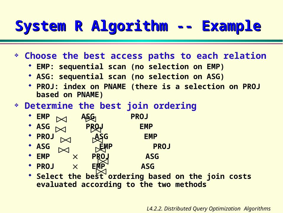
Choose the best access paths to each relation EMP: sequential scan (no selection on EMP) ASG: sequential scan (no selection on ASG) PROJ: index on PNAME (there is a selection on
PROJ based on PNAME) Determine the best join ordering
EMP ASG PROJ ASG PROJ EMP PROJ ASG EMP ASG EMP PROJ EMP PROJ ASG PROJ EMP ASG Select the best ordering based on the join costs
evaluated according to the two methods
L4.2.2. Distributed Query Optimization Algorithms -- 5
System R Example (cont'd) System R Example (cont'd)
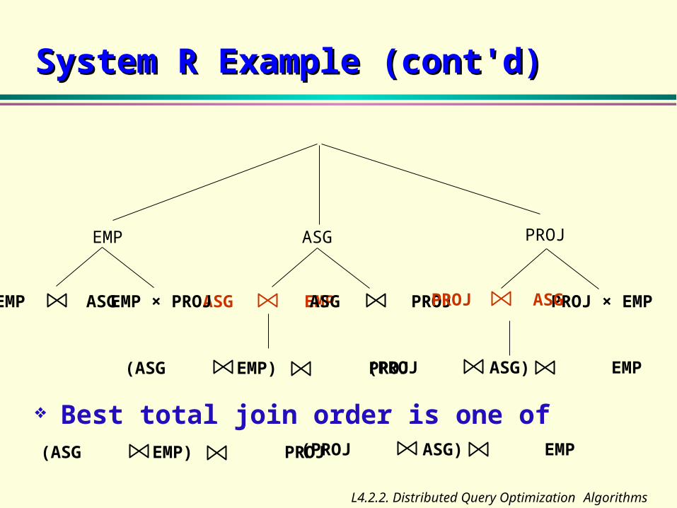
Best total join order is one of
EMP ASG PROJ
EMP ASG ASG EMP PROJ × EMPASG PROJEMP × PROJ
(ASG EMP) PROJ (PROJ ASG) EMP
PROJ ASG
(ASG EMP) PROJ (PROJ ASG) EMP
L4.2.2. Distributed Query Optimization Algorithms -- 6
System R Algorithm System R Algorithm
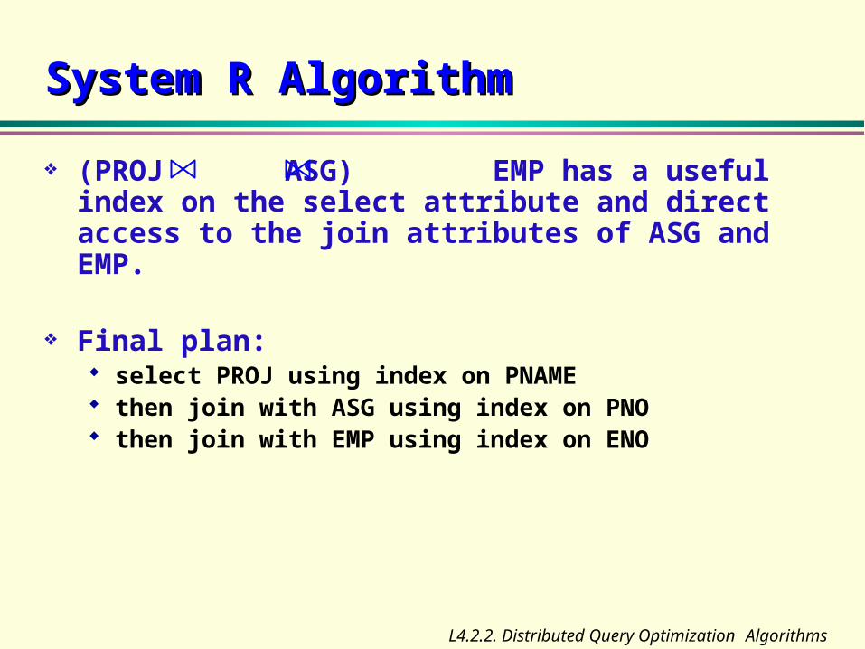
(PROJ ASG) EMP has a useful index on the select attribute and direct access to the join attributes of ASG and EMP.
Final plan:
select PROJ using index on PNAME then join with ASG using index on PNO then join with EMP using index on ENO
L4.2.2. Distributed Query Optimization Algorithms -- 7
System R* Distributed Query System R* Distributed Query OptimizationOptimization Total-cost minimization. Cost function
includes local processing as well as transmission.
Algorithm For each relation in query tree find the
best access path For the join of n relations find the optimal
join order strategy each local site optimizes the local query
processing
L4.2.2. Distributed Query Optimization Algorithms -- 8
Data Transfer StrategiesData Transfer Strategies
Ship-whole. entire relation is shipped and stored as temporary relation. If merge join algorithm is used, no need for temporary storage, and can be done in pipeline mode
Fetch-as-needed. this method is equivalent to semijoin of the inner relation with the outer relation tuple
L4.2.2. Distributed Query Optimization Algorithms -- 9
Join Strategy 1Join Strategy 1
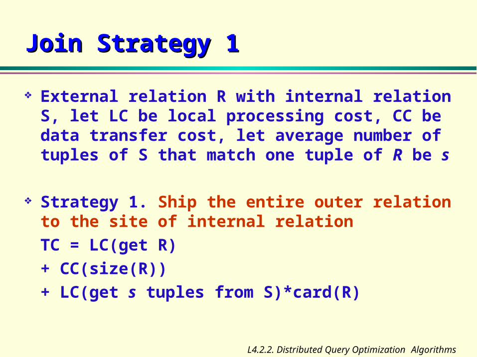
External relation R with internal relation S, let LC be local processing cost, CC be data transfer cost, let average number of tuples of S that match one tuple of R be s
Strategy 1. Ship the entire outer relation to the site of internal relationTC = LC(get R)
+ CC(size(R)) + LC(get s tuples from S)*card(R)
L4.2.2. Distributed Query Optimization Algorithms -- 10
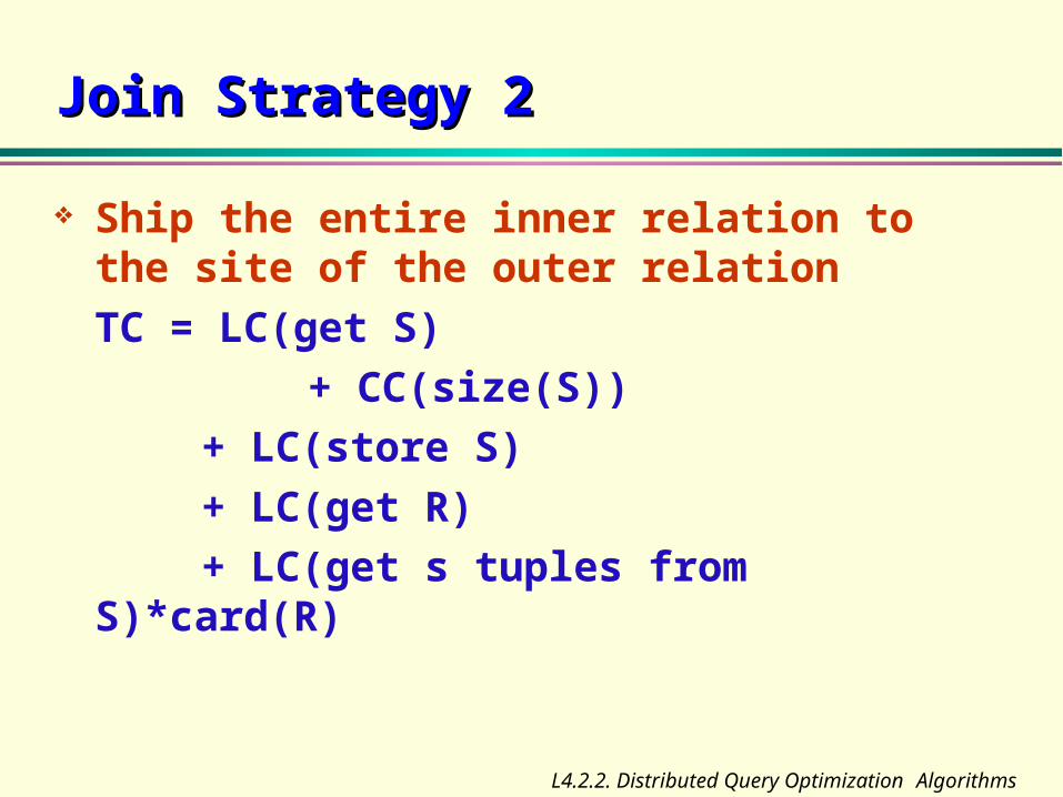
Join Strategy 2Join Strategy 2
Ship the entire inner relation to the site of the outer relationTC = LC(get S)
+ CC(size(S)) + LC(store S) + LC(get R) + LC(get s tuples from S)*card(R)
L4.2.2. Distributed Query Optimization Algorithms -- 11
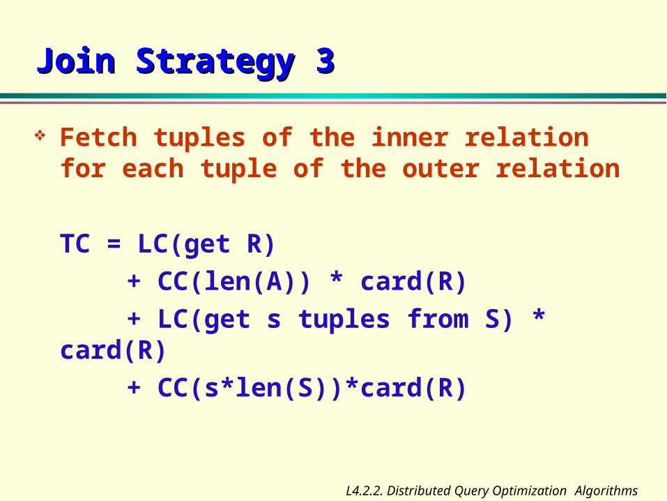
Join Strategy 3Join Strategy 3
Fetch tuples of the inner relation for each tuple of the outer relation
TC = LC(get R) + CC(len(A)) * card(R) + LC(get s tuples from S) *
card(R)+ CC(s*len(S))*card(R)
L4.2.2. Distributed Query Optimization Algorithms -- 12
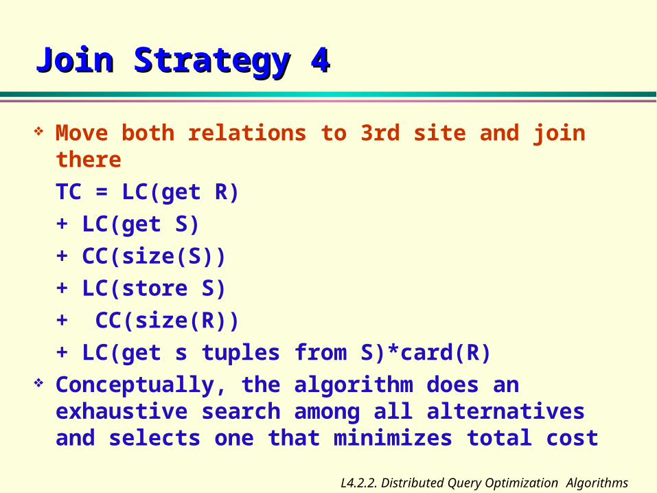
Join Strategy 4Join Strategy 4
Move both relations to 3rd site and join thereTC = LC(get R)
+ LC(get S) + CC(size(S)) + LC(store S) + CC(size(R)) + LC(get s tuples from S)*card(R)
Conceptually, the algorithm does an exhaustive search among all alternatives and selects one that minimizes total cost
L4.2.2. Distributed Query Optimization Algorithms -- 13
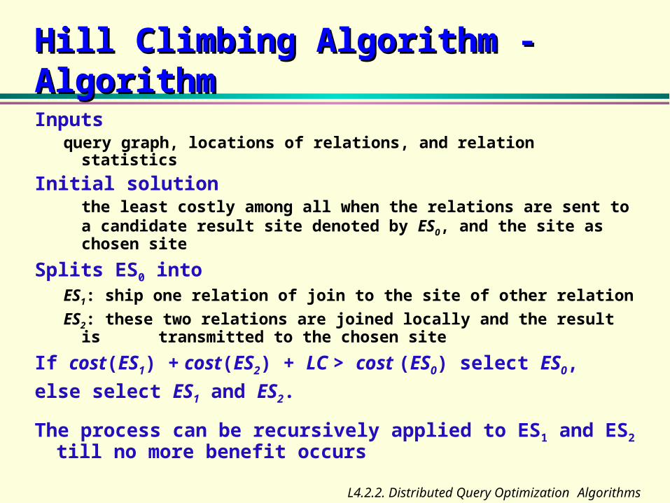
Hill Climbing Algorithm - Hill Climbing Algorithm - AlgorithmAlgorithmInputs
query graph, locations of relations, and relation statistics
Initial solution the least costly among all when the relations are sent to a
candidate result site denoted by ES0, and the site as chosen site
Splits ES0 intoES1: ship one relation of join to the site of other relation
ES2: these two relations are joined locally and the result is transmitted to the chosen site
If cost(ES1) + cost(ES2) + LC > cost (ES0) select ES0,
else select ES1 and ES2.
The process can be recursively applied to ES1 and ES2 till no more benefit occurs
L4.2.2. Distributed Query Optimization Algorithms -- 14
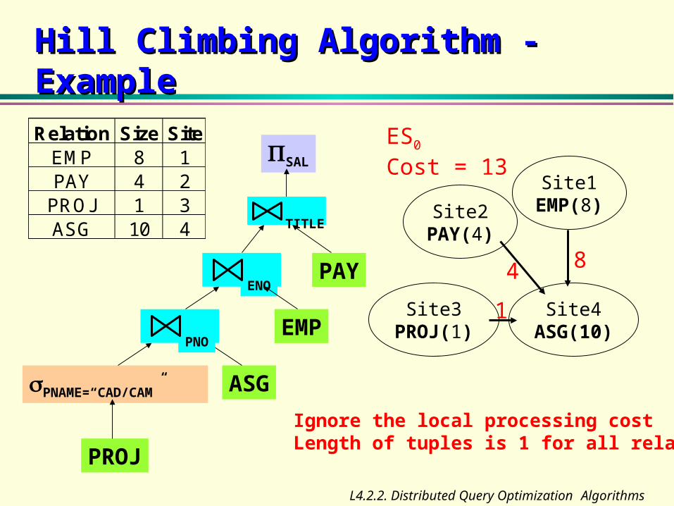
Hill Climbing Algorithm - Hill Climbing Algorithm - ExampleExample
SAL
PNAME=“CAD/CAM”
PROJ
ASG
EMPPNO
TITLE
ENOPAY
Relation Size SiteEMP 8 1PAY 4 2PROJ 1 3ASG 10 4
Ignore the local processing costLength of tuples is 1 for all relation
Site1EMP(8)Site2
PAY(4)
Site3PROJ(1)
Site4ASG(10)
ES0
Cost = 13
84
1
L4.2.2. Distributed Query Optimization Algorithms -- 15
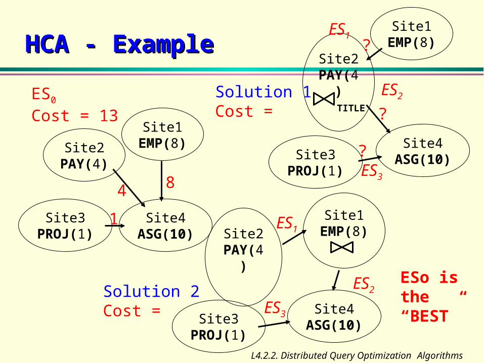
HCA - ExampleHCA - ExampleSite1
EMP(8)Site2
PAY(4)
Site3PROJ(1)
Site4ASG(10)
?
?
?
TITLE
ES1
ES2
ES3
Site1EMP(8)
Site2PAY(4)
Site3PROJ(1)
Site4ASG(10)
Site1EMP(8)Site2
PAY(4)
Site3PROJ(1)
Site4ASG(10)
ES0
Cost = 13
84
1
Solution 1Cost =
Solution 2Cost =
ES1
ES2
ES3
ESo is the “BEST”
L4.2.2. Distributed Query Optimization Algorithms -- 16
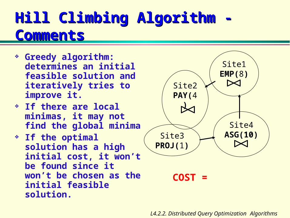
Hill Climbing Algorithm - Hill Climbing Algorithm - CommentsComments Greedy algorithm:
determines an initial feasible solution and iteratively tries to improve it.
If there are local minimas, it may not find the global minima
If the optimal solution has a high initial cost, it won’t be found since it won’t be chosen as the initial feasible solution.
Site1EMP(8)
Site2PAY(4)
Site3PROJ(1)
Site4ASG(10)
COST =
L4.2.2. Distributed Query Optimization Algorithms -- 17
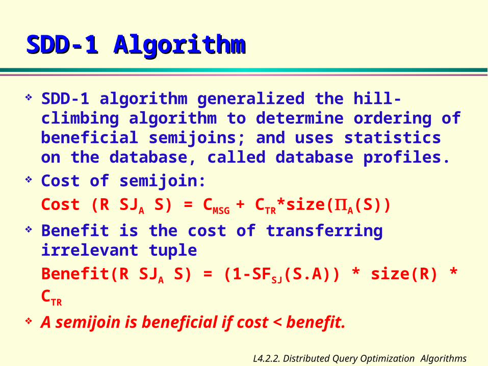
SDD-1 AlgorithmSDD-1 Algorithm
SDD-1 algorithm generalized the hill-climbing algorithm to determine ordering of beneficial semijoins; and uses statistics on the database, called database profiles.
Cost of semijoin:Cost (R SJA S) = CMSG + CTR*size(A(S))
Benefit is the cost of transferring irrelevant tupleBenefit(R SJA S) = (1-SFSJ(S.A)) * size(R) * CTR
A semijoin is beneficial if cost < benefit.
L4.2.2. Distributed Query Optimization Algorithms -- 18
SDD-1: The AlgorithmSDD-1: The Algorithm
initialization phase generates all beneficial semijoins, and an execution strategy that includes only local processing
most beneficial semijoin is selected; statistics are modified and new beneficial semijoins are selected
the above step is done until no more beneficial joins are left
assembly site selection to perform local operations
postoptimization removes unnecessary semijoins
L4.2.2. Distributed Query Optimization Algorithms -- 19
SDD1 - ExampleSDD1 - Example
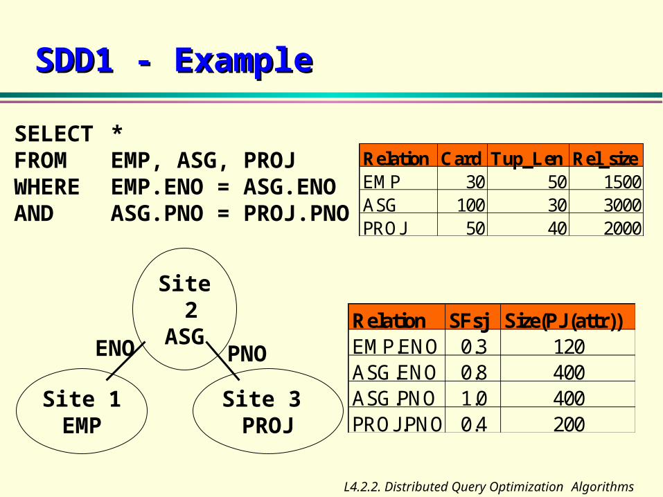
SELECT *FROM EMP, ASG, PROJWHERE EMP.ENO = ASG.ENOAND ASG.PNO = PROJ.PNO
Site 1EMP
Site 2 ASG
Site 3 PROJ
ENO PNO
Relation Card Tup_Len Rel_sizeEMP 30 50 1500ASG 100 30 3000PROJ 50 40 2000
Relation SFsj Size(PJ(attr))EMP.ENO 0.3 120ASG.ENO 0.8 400ASG.PNO 1.0 400PROJ.PNO 0.4 200
L4.2.2. Distributed Query Optimization Algorithms -- 20
SDD1 - First IterationSDD1 - First Iteration
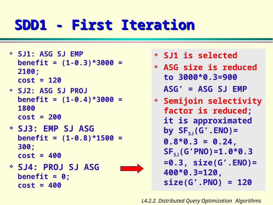
SJ1: ASG SJ EMPbenefit = (1-0.3)*3000 = 2100; cost = 120
SJ2: ASG SJ PROJbenefit = (1-0.4)*3000 = 1800cost = 200
SJ3: EMP SJ ASGbenefit = (1-0.8)*1500 = 300; cost = 400
SJ4: PROJ SJ ASGbenefit = 0; cost = 400
SJ1 is selected ASG size is reduced
to 3000*0.3=900 ASG’ = ASG SJ EMP Semijoin selectivity
factor is reduced; it is approximated by SFSJ(G’.ENO)= 0.8*0.3 = 0.24, SFSJ(G’PNO)=1.0*0.3 =0.3, size(G’.ENO)= 400*0.3=120, size(G’.PNO) = 120
L4.2.2. Distributed Query Optimization Algorithms -- 21
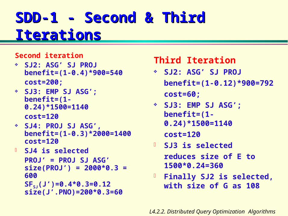
SDD-1 - Second & Third SDD-1 - Second & Third IterationsIterationsSecond iteration SJ2: ASG’ SJ PROJ
benefit=(1-0.4)*900=540cost=200;
SJ3: EMP SJ ASG’; benefit=(1-0.24)*1500=1140cost=120
SJ4: PROJ SJ ASG’, benefit=(1-0.3)*2000=1400cost=120
SJ4 is selectedPROJ’ = PROJ SJ ASG’ size(PROJ’) = 2000*0.3 = 600SFSJ(J’)=0.4*0.3=0.12size(J’.PNO)=200*0.3=60
Third Iteration SJ2: ASG’ SJ PROJ
benefit=(1-0.12)*900=792cost=60;
SJ3: EMP SJ ASG’; benefit=(1-0.24)*1500=1140cost=120
SJ3 is selected reduces size of E to
1500*0.24=360 Finally SJ2 is selected,
with size of G as 108
L4.2.2. Distributed Query Optimization Algorithms -- 22
Local OptimizationLocal Optimization
Each site optimizes the plan to be executed at the site
A centralized query optimization problem
L4.2.2. Distributed Query Optimization Algorithms -- 23
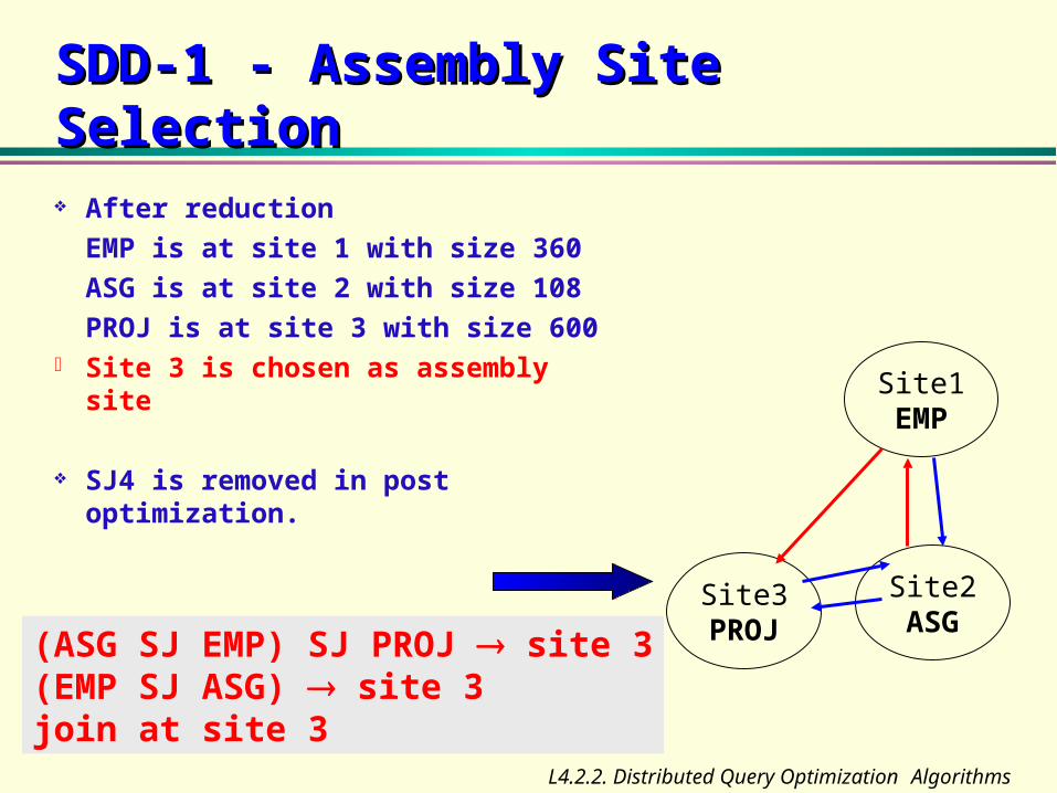
SDD-1 - Assembly Site SDD-1 - Assembly Site SelectionSelection After reduction
EMP is at site 1 with size 360ASG is at site 2 with size 108PROJ is at site 3 with size 600
Site 3 is chosen as assembly site
SJ4 is removed in post optimization.
Site1EMP
Site3PROJ
Site2ASG
(ASG SJ EMP) SJ PROJ site 3(EMP SJ ASG) site 3join at site 3