L3 Latency in Regional Networks - Theseus
120
L3 Latency in Regional Networks Preparing 5G Launch Markus Ruotsalainen Bachelor’s thesis May 2018 Technology, Communication and Transport Degree Programme in Information and Communications Technology
Transcript of L3 Latency in Regional Networks - Theseus
L3 Latency in Regional Networks Preparing 5G Launch
Markus Ruotsalainen
Bachelor’s thesis May 2018 Technology, Communication and Transport Degree Programme in Information and Communications Technology
Description
Author(s)
Ruotsalainen, Markus Type of publication
Bachelor’s thesis Date
15.05.2018
Language of publication English
Number of pages
117 Permission for web publi-
cation: yes
Title of publication
L3 Latency in Regional Networks Preparing 5G launch
Degree programme
Degree Programme in Information and Communications Technology
Supervisor(s)
Kotikoski Sampo, Häkkinen Antti
Assigned by
Telia Finland Oyj
Abstract
The purpose of the research was to measure the two-way L3 latency in Telia Finland’s re-gional MPLS networks. The subject was topical, as 5G networks require a significantly smaller amount of delay compared to the existing 4G mobile networks. The primary objec-tive was to produce a baseline for the network delay to be used in planning and develop-ment of the regional networks to prepare for the introduction of 5G.
An additional objective was to compare two measurement methods to determine their suitability for conducting measurements in the production network. Eventually ping was selected as a measurement method while TWAMP implementation was limited solely to Telia’s laboratory environment. However, the results gained from TWAMP testing were used as a reference when assessing the reliability of the results measured from production network.
The research constrained to Telia’s 13 regional networks consisting of Nokia’s SR, ESS, and SAS series routers and switches. In total, 1139 network elements were measured using fping program run on a Unix server in a separate management network. In order to assess the reliability of the results, additional data gained with traceroute program as well as in-ventory information such as location and site details was combined with the actual meas-urement data.
The result of the research was a reliability analysis of the measurement statistics and the baseline delivered to designers responsible for planning the regional networks. Despite the fact that ICMP traffic is de-prioritized in network elements, this research proves that a sim-ple measurement method can produce accurate enough information for planning and can reveal issues in the network.
Keywords/tags (subjects)
regional network, latency, delay, ping, ICMP, TWAMP, TWAMP Light, Nokia, SR, ESS, SAS, 5G Miscellaneous

Kuvailulehti
Tekijät(t)
Ruotsalainen, Markus Julkaisun laji
Opinnäytetyö, AMK Päivämäärä
15.05.2018
Julkaisun kieli Englanti
Sivumäärä
117 Verkkojulkaisulupa myön-
netty: kyllä
Työn nimi
L3 Latency in Regional Networks Preparing 5G launch
Tutkinto-ohjelma
Tietotekniikka
Työn ohjaaja(t)
Sampo Kotikoski, Antti Häkkinen
Toimeksiantaja(t)
Telia Finland Oyj
Tiivistelmä
Tutkimuksen tavoitteena oli mitata kaksisuuntainen L3-viive Telia Finland Oyj:n MPLS-alueverkossa. Tutkittava aihe oli ajankohtainen, sillä 5G-verkon käyttöönotto vaatii ope-raattorin runkoverolta huomattavasti pienempää viivettä nykyiseen 4G-standardiin verrat-tuna. Pääasiallisena tavoitteena oli tuottaa tieto tuotantoverkon viiveistä viiveen vertai-luarvojen tuottamiseksi, jolloin vertailuarvoja voidaan hyödyntää alueverkkojen suunnitte-lussa ja rakentamisessa 5G-verkon käyttöönottoa varten.
Tutkimuksessa tarkasteltiin lisäksi kahta eri mittausmenetelmää, jolloin menetelmistä sopi-vampi voitiin valita tuotantoverkon viivemittauksiin. Lopulliseksi mittausmenetelmäksi vali-koitui ICMP-protokollaan perustuva ping ja TWAMP-protokollaa päädyttiin testaamaan ai-noastaan Telian laboratorioympäristössä. TWAMP-protokollalla saatuja mittaustuloksia käytettiin kuitenkin tuotantoverkosta mitattujen viiveitten luotattavuuden arviointiin.
Mittaus rajoittui Telian 13 alueverkkoon, jotka koostuivat Nokian SR-, ESS- ja SAS-sarjan reitittimistä ja kytkimistä. Mittaukset toteutettiin fping-sovelluksella, jota ajettiin hallinta-verkossa sijaitsevalta Unix-palvelimelta, ja mittaukset kohdistuivat yhteensä 1139 verkko-laitteeseen. Tulosten analysoinnin helpottamiseksi mittaustuloksiin yhdistettiin lisäksi lai-tetietokannan sijainti- ja teletilatietoja sekä traceroute-sovelluksella kerättyä dataa.
Työn lopputuloksena oli arvio mittaustulosten luotettavuudesta sekä taulukoitu viivestatis-tiikka, joka luovutettiin alueverkon suunnittelijoiden käyttöön. Siitä huolimatta että verk-kolaitteet käsittelevät ICMP-liikennettä muuta liikennettä alemmalla prioriteetilla, tutki-mus osoittaa, että yksinkertainen mittausmenetelmä voi tuottaa riittävän tarkkaa tietoa suunnittelutyöhön sekä paljastaa lisäksi verkon ongelmakohtia.
Avainsanat (asiasanat)
alueverkko, viive, ping, ICMP, TWAMP, TWAMP Light, Nokia, SR, ESS, SAS, 5G Muut tiedot

1
Contents
Acronyms ............................................................................................................... 6
1 Introduction ................................................................................................... 9
2 Research Frame ............................................................................................ 11
3 Telia Company .............................................................................................. 12
4 IP Network ................................................................................................... 14
4.1 General Design of Large-Scale IP Networks .............................................. 14
4.2 TCP/IP Model ............................................................................................. 18
5 Telia Network Architecture ........................................................................... 25
5.1 Backbone Networks................................................................................... 25
5.2 Regional Network ...................................................................................... 28
5.2.1 Topology ............................................................................................... 28
5.2.2 Traffic Forwarding................................................................................. 31
5.3 Access Network ......................................................................................... 34
6 5G ................................................................................................................ 36
7 Network Performance .................................................................................. 39
7.1 Metrics ....................................................................................................... 39
7.2 Network Delay ........................................................................................... 41
7.3 Delay Variation .......................................................................................... 45
8 Performance Monitoring Methods ................................................................ 46
8.1 Overview .................................................................................................... 46
8.2 Ping ............................................................................................................ 48
8.2.1 Basic Operation ..................................................................................... 48
8.2.2 Reliability .............................................................................................. 51
8.3 TWAMP ...................................................................................................... 53
8.3.1 Overview ............................................................................................... 53
8.3.2 TWAMP-Control .................................................................................... 56
8.3.3 TWAMP-Test ......................................................................................... 61
8.3.4 TWAMP Light ........................................................................................ 64
9 TWAMP Implementation .............................................................................. 66
9.1 TWAMP Light ............................................................................................. 66
9.1.1 Preparation ........................................................................................... 66
9.1.2 MPLS and BGP....................................................................................... 67

2
9.1.3 VPRN ..................................................................................................... 70
9.1.4 Controller and Reflector ....................................................................... 73
9.2 TWAMP ...................................................................................................... 76
9.3 Comparison of TWAMP Light and ping ..................................................... 80
10 Latency Tests ................................................................................................ 83
10.1 Preparation ................................................................................................ 83
10.2 fping ........................................................................................................... 85
11 Results ......................................................................................................... 88
11.1 Analysis ...................................................................................................... 88
11.2 Conclusions ................................................................................................ 95
11.3 Improvements and Recommendations ..................................................... 96
12 Discussion .................................................................................................... 98
References ......................................................................................................... 101
Appendices ........................................................................................................ 106

3
Figures
Figure 1. Mobile Data Growth Estimation ..................................................................... 9
Figure 2. IP-over-WDM ................................................................................................. 15
Figure 3. Architecture of Internet ................................................................................ 16
Figure 4. Modular Large Scale Network ....................................................................... 17
Figure 5. TCP/IP Layers ................................................................................................. 20
Figure 6. IP Header ....................................................................................................... 22
Figure 7. Encapsulation Process ................................................................................... 24
Figure 8. TCP/IP – Basic Philosophy ............................................................................. 25
Figure 9. International Network ................................................................................... 26
Figure 10. Inter-regional Network ................................................................................ 27
Figure 11. Logical Topologies ....................................................................................... 29
Figure 12. Regional Network ........................................................................................ 30
Figure 13. IS-IS Areas and Metrics ................................................................................ 32
Figure 14. Encoding of the MPLS Label Stack............................................................... 33
Figure 15. LSP Example ................................................................................................. 34
Figure 16. Service Forwarding and Encapsulation ....................................................... 36
Figure 17. Enhancement of Key Capabilities from IMT-Advanced to IMT-2020 ......... 37
Figure 18. IMT-2020 Usage Scenarios .......................................................................... 38
Figure 19. End-to-end Transfer of an IP Packet ........................................................... 44
Figure 20. End-to-end 2-Point IP Packet Delay ............................................................ 46
Figure 21. ICMP Echo Query and Response ................................................................. 49
Figure 22. ICMP Echo/Reply Header ............................................................................ 50
Figure 23. General Router Architecture ....................................................................... 51
Figure 24. Logical Structure of TWAMP ....................................................................... 55
Figure 25. Roles of the TWAMP Hosts ......................................................................... 55
Figure 26. Server-Greeting Message ............................................................................ 57
Figure 27. Set-Up-Response Message .......................................................................... 58
Figure 28. Server-Start Message .................................................................................. 59

4
Figure 29. TWAMP-Control Commands ....................................................................... 60
Figure 30. Accept-Session Message ............................................................................. 61
Figure 31. TWAMP Test Packet Format I ..................................................................... 62
Figure 32. TWAMP Test Packet Format II .................................................................... 64
Figure 33. TWAMP Light: Controller and Responder Roles ......................................... 65
Figure 34. VSR Topology ............................................................................................... 67
Figure 35. BGP Configuration Prerequisites ................................................................. 69
Figure 36. TWAMP Light Test Session (VPRN) .............................................................. 71
Figure 37. Reflector Connectivity Test ......................................................................... 72
Figure 38. Reflector Statistics ....................................................................................... 76
Figure 39. TWAMP Light Test Session (TWAMP server) .............................................. 77
Figure 40. TWAMP Test Instance in 5620 SAM ............................................................ 78
Figure 41. TWAMP Server Status ................................................................................. 79
Figure 42. Comparison of Round-trip Delay (TWAMP Light and ping) ........................ 80
Figure 43. TWAMP Light Test Sessions ........................................................................ 81
Figure 44. Measurement Topology I ............................................................................ 85
Figure 45. Measurement Topology II ........................................................................... 86
Figure 46. Round-trip Delay Statistics .......................................................................... 88
Figure 47. Comparison of Round-trip Delay Statistics ................................................. 90
Figure 48. Delay Components I .................................................................................... 91
Figure 49. Delay Components II ................................................................................... 92
Figure 50. Comparison of Round-trip Delay Statistics (Theoretical vs. Actual) I ......... 94
Figure 51. Comparison of Round-trip Delay Statistics (Theoretical vs. Actual) II ........ 94
Tables
Table 1. Regional Network Nodes ................................................................................ 28
Table 2. Telia Carrier’s Performance Report – March 2018......................................... 43
Table 3. ICMP Message Types ...................................................................................... 50
Table 4. Comparison of TWAMP and Ping ................................................................... 53

5
Table 5. Physical Equipment ........................................................................................ 77
Table 6. Round-trip Delay (TWAMP Light) ................................................................... 82
Table 7. Round-trip Delay (Ping) .................................................................................. 82
Table 8. ME Node Response Rates within Time Intervals ............................................ 93

6
Acronyms
3GPP 3rd Generation Partnership Project
4G 4th Generation
5G 5th Generation
ASBR Autonomous System Border Router
AES Advanced Encryption Standard
BGP Border Gateway Protocol
CLI Command Line Interface
CPE Customer Premises Equipment
CPU Central Processing Unit
DNS Domain Name System
DSLAM Digital Subscriber Line Access Multiplexer
eMBB Enhanced Mobile Broadband
ESS Ethernet Service Switch
FEC Forwarding Equivalence Class
FTTB Fiber to the Building
ICMP Internet Control Message Protocol
IGP Interior Gateway Protocol
IP Internet Protocol
IPTD IP Packet Transfer Delay
ITU International Telecommunication Union
IS-IS Intermediate System-to-Intermediate System
ISP Internet Service Provider
L2 Layer 2
L3 Layer 3

7
LAN Local Area Network
LSP Label Switched Path
LSR Label Switching Router
MBH Mobile Backhaul
ME Metro Ethernet
MEF Metro Ethernet Forum
mMTC Massive Machine Type Communications
MPLS Multiprotocol Label Switching
NR New Radio
NSE Network Section Ensemble
NTP Network Time Protocol
OAM Operation Administration and Maintenance
OWAMP One-Way Active Measurement Protocol
PDU Protocol Data Unit
PE Provider Edge
PM Performance Management
POP Point of Presence
QoS Quality of Service
SAM Service Aware Manager
SAP Service Access Point
SAS Service Access Switch
SLA Service Level Agreement
SR Service Router
SR OS Service Router Operating System
SNMP Simple Network Management Protocol
TCC TWAMP and TWAMP-Light Control Client

8
TCP Transport Control Protocol
TOS Type of Service
TTL Time to Live
TWAMP Two-way Active Measurement Protocol
UDP User Datagram Protocol
uRLLC Ultra-Reliable and Low-latency Communications
VPN Virtual Private Network
VPRN Virtual Private Routed Network
VRF Virtual Routing and Forwarding
VSR Virtual Service Router
WDM Wavelength Division Multiplexing

9
1 Introduction
In the course of the history of the Internet, organizations have not always been confi-
dent to rely on network services for business critical tasks, due to bottlenecks relat-
ing to lack of routing intelligence and bandwidth issues. Over the years, the develop-
ment of networks has led to significant service quality improvements with increased
bandwidth capacity and overall reliability. The Internet Protocol has become an inte-
gral part of people’s everyday lives that allows carrying data, voice and video in-
stantly around the world. (Service Level Monitoring with Cisco IOS Service Assurance
Agent N.d.)
General adoption of IP (Internet Protocol) has caused a significant increase in overall
data traffic. Today, as mobile devices have become a commodity, the trend is the
mobile Internet. According to Cisco’s VNI Forecast Highlights Tool (N.d.), the overall
monthly IP data traffic will almost triple its byte-count in 2021. Regarding mobile net-
works, the mobile data will grow globally 7-fold from 2016 to 2021. This can be seen
in Figure 1, which presents the estimation for global mobile data growth in exabytes
between 2016 and 2021.
Figure 1. Mobile Data Growth Estimation (VNI Forecast Highlights Tool N.d.)

10
The evolution of IP networks does not seem to slow down, as new types of applica-
tions and services are brought to mobile devices. As the mobile Internet has become
more common access technology, also the expectations towards the performance of
mobile networks have raised. To meet the demands for high-speed mobile subscrip-
tions and better user experience, service providers need to respond by introducing
new wireless technologies to their customers.
The upcoming 5G (5th Generation) aims to enhance the capabilities of today’s 4G (4th
Generation) mobile networks by providing more throughput and better QoS (Quality
of Service). 5G also extends the service range by introducing new applications includ-
ing wearable devices, platforms for IoT (Internet of Things), high quality video
streams and autonomous vehicles. Each of the applications require certain capabili-
ties from the network infrastructure such as energy efficiency, throughput or latency.
Although the overall mobile data is expected to multiply in the future, the through-
put is not the only important metric for defining network performance.
The commercialization of 5G networks requires that existing network infrastructure
can meet all of the specifications set for 5G services. Probably the most problematic
metric for the next generation mobile network is the latency, which is especially im-
portant to uRLLC (Ultra-Reliable and Low-latency Communications) 5G applications
such as healthcare management devices or self-driving cars. These applications re-
quire 1 millisecond latency, which in practice, is equal to the distance light impulse
travels approximately 200 kilometers in the glass core of an optical fiber.
The length of the transmission medium is one of the dominant factors contributing
to overall latency meaning the distance constraints the 5G architecture. The other
factor contributing to overall latency is the equipment. Each time the data passes
through a router or switch, the latency increases as IP packets need to be processes

11
by the equipment. Although 5G’s uRLLC applications are not the first to be intro-
duced as a service, it is essential to determine the latency of the network to prepare
for 5G era. This is important especially when network infrastructure forms a country-
wide large-scale network consisting of hundreds or thousands of Metro Ethernet
nodes.
2 Research Frame
The primary objective of this thesis is to provide a baseline for L3 (Layer 3) latency in
Telia’s Finnish regional networks. The baseline is used to determine, if the current
state of regional networks meet the latency requirements set for 5G services. This in-
formation is important to the organization as the baseline is expected to indicate the
parts of regional networks, which might require investments from the organization.
The study does not take a stand on whether construction of regional networks is nec-
essary but only aims to provide the latency statistics for Telia organization. The main
research question is “How high is the latency in regional networks?”
This thesis follows a quantitative research approach in latency measurements since
the data requires analyzation of the numeric data. According to Shuttleworth (N.d.),
quantitative experiments suit research which uses mathematical or statistical means
to solve research questions. Additionally, the benefits of a quantitative research ap-
proach is that the research can be repeated if they are constructed correctly (Shuttle-
worth N.d.). While the measurement statistics are analyzed as quantitative means,
the study also contains a minor qualitative element, as it aims to study how to effec-
tively conduct the measurements. The analyzation of the data gained is based pri-
marily on quantitative research calculations, and mathematical comparison of the
data gained from individual measurement sessions.

12
Two main factors constraint this study. The first constraint is the equipment used in
regional networks. The research focuses only on the part of regional networks con-
sisting of Nokia’s SR (Service Router), ESS (Ethernet Service Switch) and SAS (Service
Access Switch) series equipment forming the main backbone for 13 individual re-
gional networks. The total amount of routers and switches in the scope is 1139 de-
vices.
The second constraint are the measurement methods. The thesis focuses on ping
and TWAMP (Two-way Active Measurement Protocol). Ping was selected as it is a
common program available in the most of network hosts and provides an accurate
enough baseline for the regional latency. TWAMP, on the other hand, was selected,
since it is not yet implemented in Telia’s regional networks; and in theory, provides
more exact delay statistics over ping. Since there is not much comprehensive re-
search data or publications concerning TWAMP, testing it may provide additional in-
formation when TWAMP is adopted as a measurement method in regional networks.
3 Telia Company
Telia Company has roots in history all the way back to the telegraph age in the 19th
century – long before the merger of the two companies, Swedish Telia and Finnish
Sonera took place. Before merging into TeliaSonera, the underlying histories of both
countries have much in common although some important differences exist. Telia’s
home country Sweden has enjoyed a long period of peace after the Treaty of Hamina
that ended the Finnish War between Sweden and the Russian Empire in 1809. As a
part of the treaty conditions Sweden had to cede the whole of Finland to Russia,
which in contrast, meant more turbulence for telecom development in Finland.
(Geary, Martin-Löf, Sundelius & Thorngren 2010, 7.)

13
The roots of Telia reach to its home country Sweden, where its predecessor Telever-
ket was originally formed to run the electrical telegraph in Sweden in 1853. After the
arrival of telephone in the 1880s, Televerket received competition as local private
companies started to build telephone networks. Eventually, the majority of the local
telephone networks fell under Televerket’s control when the Swedish government
decided to build a united national telephony network. In the early 20th century,
Televerket finally achieved the monopoly status by purchasing the largest competitor
Stockholms-telefon in the early 20th century and the telecommunications in Sweden
came under state control. (Geary et al. 2010, 7.)
In Sweden’s neighboring country Finland, the results of the Finnish War affected sig-
nificantly the local telecommunication systems. During the era when Finland was a
Russian Grand Duchy, the Finnish Telegraph was a part of Imperial Telegraph. Be-
tween 1855 and 1917, the telegraph remained under Russian control; yet, the re-
gional telephone networks were secured by private companies wanting to protect
Finnish autonomy. After the declaration of Finnish independence, the state-owned
Finnish Telegraph Administration was formed to take control over the telegraph sys-
tem and only some parts of fixed telephony in Finland. During the 20th century, the
local telecom business was mainly in the hands of many private monopoly compa-
nies. Unlike in Sweden, the Finnish telecommunication market was divided roughly
into two equally-sized segments, and thus, it was never a responsibility of any single
entity. (Geary et al. 2010, 7-8.)
Technologically-wise, the years through 1970s – 1980s were important in the Nordic
countries since the telephony network became fully automated, the first mobile gen-
eration (1G) was introduced and the transmission lines were digitalized in 1987. The
Finnish and Swedish national telecom authorities continued developing individually;

14
however, they started to cooperate in the Baltic region in 1990s. They were eventu-
ally listed on the stock exchange and two companies were founded. The telecom au-
thority in Sweden became Telia AB and the Finnish counterpart became Sonera Oy.
In 2002, the companies merged as TeliaSonera after Sonera’s financial crisis resulted
from failed 3G technology investments in Germany. (10 Year Review of TeliaSonera
2013.)
Today, Telia Company is the fifth largest network operator in the Europe, which pro-
vides network access and telecommunication services in 12 countries including the
Nordic and Baltic countries as well as in Eurasia. At the end of year 2017, Telia had
23.1 million active subscriptions and in total 20 700 employees. Telia’s service portfo-
lio includes wide range of products and services for operator, enterprise and residen-
tial customer segments. The current strategy of the company is to invest in capacity
in order to secure high quality transportation of massive data volumes and network
virtualization to achieve a converged IT infrastructure. (Annual and Sustainability Re-
port 2017, 4-7 and 21.)
4 IP Network
4.1 General Design of Large-Scale IP Networks
Certainly, the best known large-scale IP network is the Internet of today. The Internet
is a collection of interlinked independent service provider networks, which provide a
global medium for users and devices around the world. These independent networks
are run by different companies and organizations sharing common protocols and
network architecture in order to operate together. Two main elements form the In-
ternet: communication links that transport the data from one point to another and
routers, which direct the traffic flow between the links. (Nucci & Papagiannaki 2009.)

15
Communication links may vary from telephone lines to television system cables, or to
wireless circuits including satellite or radio link connections. In the developed part of
the world, links that carry the large amounts of Internet traffic are optical fiber ca-
bles. The largest of these high capacity links form the backbone for the Internet and
may be directly owned by ISPs (Internet Service Provider) or by organizations that of-
fer link capacity to network operators. As backbone networks require high capacity
and high performance, they utilize IP-over-WDM (Wavelength Division Multiplexing)
technology to bundle multiple signals together. In IP-over-WDM, the physical optics
provide a medium for logical IP links between network nodes as shown in Figure 2.
(Nucci et al. 2009.)
Figure 2. IP-over-WDM (Nucci et al. 2009)
The Internet consists of ISPs categorized into three different tiers and each of them
administers their own share of the global IP network. Figure 3 illustrates a hierarchic
ISP relationships model, which describes transit and peering interconnection princi-
ples between tiers. According to Ghafary, Shaheen & Warnock (2015), there are not

16
hard distinction between the tiers, but the following generally accepted definitions
apply:
A tier 1 ISP can reach any part of Internet without paying transit fees and therefore must peer with all other tier 1 ISPs.
A tier 2 does not have the same global reach as tier 1 ISP, but rather serves large regional area such as a country or continent. A tier 2 ISP peers with other tier 2 ISPs and relies acquiring transit services from Tier 1 in order to reach the remaining parts of the Internet.
A tier 3 ISP serves small regional areas and depends solely on transit services provided by higher-tier service providers.
Figure 3. Architecture of Internet (Ghafary et al. 2015)
Although the design of the Internet breaks down to individual networks of service
providers, a tier 1 ISP network still reaches great geographical distances. According to
Raza & Turner (1999, 83-84), a successful network design of a large network bases on

17
modular network model, which divides into core (equivalent also to backbone layer),
distribution and access layers. Even though this Cisco’s theoretical model is nearly
two decades old, modern large-scale IP network design still follows this fundamental
structure due to its efficiency in packet forwarding process.
Figure 4 visualizes a high-level example of a service provider network, which follows
a three-layered hierarchical model. In the figure, the red backbone links connect the
core sites within a service provider network as well as connect the service provider
network to other service providers (peers). The core sites also connect to distribution
and access layers, which extend reachability towards customers in the edge of re-
gions.
Figure 4. Modular Large Scale Network (Modified from Raza et al. 1999, 31)

18
The network layers consist of routers performing a number of different roles de-
pending which network layer they serve. In general, a service provider network con-
sist of small number of high-capacity core routers at higher network layers and larger
number of low capacity nodes at lower layers. Core routers are responsible for con-
necting regional networks to the backbone by forwarding packets to and from the re-
gions. Core routers also advertise regional reachability information to the other core
routers and may exchange routes with external peer networks. (Raza et al. 1999, 84-
85.)
Distribution routers are used to consolidate connections from access routers and
provide redundant connections to the backbone network. Distribution routers also
may contain topological information about their own region, but they forward pack-
ets to core routers for inter-regional routing. In some cases, distribution routers may
form their own hierarchy and can be used for direct customer connections that re-
quire high-performance services. (Raza et al. 1999, 85.)
The access layer connects the remaining customers to the distribution network. Typi-
cally, the access layer consists of lower-end equipment with high port density that
collect the traffic from multiple customers using several access technologies. In
packet switched networks, it is common that access devices use Ethernet to connect
to the CPE (Customer Premises Equipment).
4.2 TCP/IP Model
Because IP networks need to support a vast amount of protocols and devices regard-
less of vendors, all Internet hosts must follow universal methods in order to com-
municate together. The principles of communication between Internet hosts have

19
been defined in Internet standard RFC 1122 Requirements for Internet Hosts -- Com-
munication Layers. According to RFC 1122 (1989, 7-8), the Internet architecture ba-
ses on network reference model where the following fundamental assumptions ap-
ply:
Internet design has to tolerate network variation including e.g. bandwidth, de-lay, packet loss and packet reordering, as well as failure of individual networks, gateways (routers) or hosts
An Internet host must be able to communicate with all other Internet hosts re-gardless of their location
Hosts must use the same set of protocols regardless of their location
Gateways are designed to be stateless and end-to-end host data flow control is implemented in hosts
Only routers should be responsible of routing actions
A network reference model is a logical structure that defines how devices and soft-
ware interoperate in multi-vendor IP networks. Although other network reference
models exist, TCP/IP model is the foundational de facto protocol today’s IP networks.
The TCP/IP model was originally sprouted when U.S. Department of Defense started
funding a reference model that would help build a network that could withstand in
crisis situations – even in case of a nuclear war. (Odom 2011.) The name TCP/IP de-
rives from two of its best known protocols TCP (Transmission Control Protocol) and
IP. Regardless of the naming convention, the TCP/IP model provides a framework for
wide array of different protocols. (Goralski 2009.)
The fundamental element of the TCP/IP model are communication protocol layers.
Each TCP/IP layer has specific functions distinct from the others; however, they can
be combined for performance reasons (Goralski 2009). Figure 5 presents the five-lay-
ered TCP/IP model where some of the common protocols used in service provider
networks are tied to the protocol layers. The figure also maps the four lowest layers
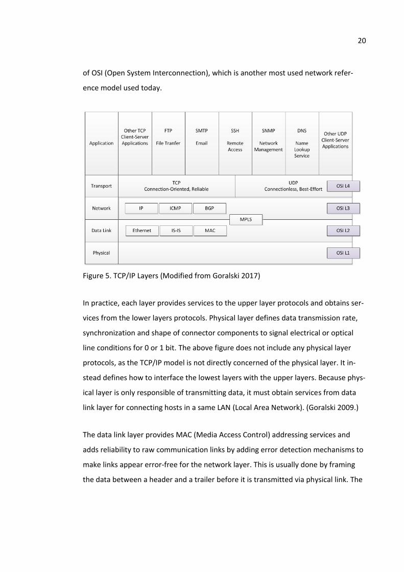
20
of OSI (Open System Interconnection), which is another most used network refer-
ence model used today.
Figure 5. TCP/IP Layers (Modified from Goralski 2017)
In practice, each layer provides services to the upper layer protocols and obtains ser-
vices from the lower layers protocols. Physical layer defines data transmission rate,
synchronization and shape of connector components to signal electrical or optical
line conditions for 0 or 1 bit. The above figure does not include any physical layer
protocols, as the TCP/IP model is not directly concerned of the physical layer. It in-
stead defines how to interface the lowest layers with the upper layers. Because phys-
ical layer is only responsible of transmitting data, it must obtain services from data
link layer for connecting hosts in a same LAN (Local Area Network). (Goralski 2009.)
The data link layer provides MAC (Media Access Control) addressing services and
adds reliability to raw communication links by adding error detection mechanisms to
make links appear error-free for the network layer. This is usually done by framing
the data between a header and a trailer before it is transmitted via physical link. The

21
data link layer cannot communicate outside LAN and relies on network layer proto-
cols. (Goralski 2009.)
The network layer includes only a few protocols, but one major protocol, IP. IP is a
widely used protocol designed to interconnect devices in packet-switched networks
by providing two important functions: addressing and routing (Odom 2011). Every In-
ternet host needs a unique network address that universally pinpoints their individ-
ual locations. For this purpose, the network layer uses IP addresses to reach distant
links and hosts across the Internet. IP does also allow other important functions like
traffic prioritization and fragmenting. By fragmenting data to packets, IP helps ensure
that packets reach to their destinations in IP networks, which are by default unrelia-
ble. (Carrell, Kim & Solomon 2015.) Figure 6 describes the original IPv4 packet for-
mat, which includes the following fields:
Version Defines the IP version (IPv4)
IHL Indicates the length of IP header
Type of Service (Type of Service field have been renamed and is currently used to define Differentiated Services Code Points)
Total Length Indicates the total Length of the IP packet including header and data
Identification Identifier assigned by the sender to aid reassembling fragments
Flags Provides additional information about fragments and can be used to prevent fragmentation
Fragment Offset Indicates the number of 8-byte units in the packet fragment
Time to Live 8-bit value which is decremented by routers are packet traverses in the network (IP packet is discarded if Time to Live reaches 0)

22
Protocol Indicates the transport layer protocol number carried in the IP packet
Options Defines rarely used optional variables not common today
Padding The amount bits that are added to the IP header to ensure header size end on a 32-bit boundary (used only if Options are used)
(Goralski 2017, 202-204.)
Figure 6. IP Header (RFC 791 1981, 11)
Because of the unreliable characteristics of the network layer, and due to the fact IP
packets are fragmented, IP packet might not always use same network path to its
destination – and there is also a possibility that it will not reach it at all. In the Inter-
net, end-to-end message delivery relies on transport layer protocols. The two of the
most common protocols at transport layer are TCP and UDP (User Datagram Proto-
col). TCP is used when it is necessary to guarantee that data flows reach their desti-
nations, whereas UDP is used when certain application (e.g. video stream) can toler-
ate some data loss. The primary functions of transport layer include error correction
mechanisms, retransmission of data as well as ensuring that transmitted data is pre-
sented to applications in the correct order. (Carrell et al. 2015.)

23
In contrast to UDP, TCP connections include a successful three-way handshake be-
tween hosts before transmission of actual application data can begin. The handshake
process is a prerequisite for some applications, such as email clients or web brows-
ers, which require a reliable host-to-host connection. This makes UDP more desirable
protocol when speed is a crucial factor and there is no need for error correction
mechanisms. The transport layer is the first layer to receive data from applications
and starting the encapsulation process required for end-to-end communication be-
tween two hosts.
Figure 7 illustrates a scenario where two hosts communicate with each other using a
five-layered TCP/IP model. In the figure, an application running on a Device A initi-
ates communication session with a remote Device B over IP network. The application
layer interacting directly with the user and the software application, passes applica-
tion data to the transport layer, which encapsulates the application data with a
transport layer header (TH) starting the encapsulation process. When the transport
layer has finished the encapsulation process, the application data is passed to lower
layers, where the data is further encapsulated within IP packets and frames before
transmission. When Device B receives the data, it removes the headers and finally
passes the data to correct application based on TCP or UDP port numbers present in
transport layer headers.

24
Figure 7. Encapsulation Process (Goralski 2009)
Not all hosts of a network need to mandatorily implement all layers of TCP/IP. The
basic philosophy of TCP/IP follows a flexible model, which allows an intermediate
system – such as a router to efficiently function only on the first three layers of
TCP/IP (Goralski 2009). As illustrated in Figure 8, the core network functions in
TCP/IP networks remain simple and efficient whereas functions of the edges of the
network surrounding the core on the other hand are more complex. This is sensible,
since the one of the main core network functionalities is to enable high-speed data
forwarding for applications.
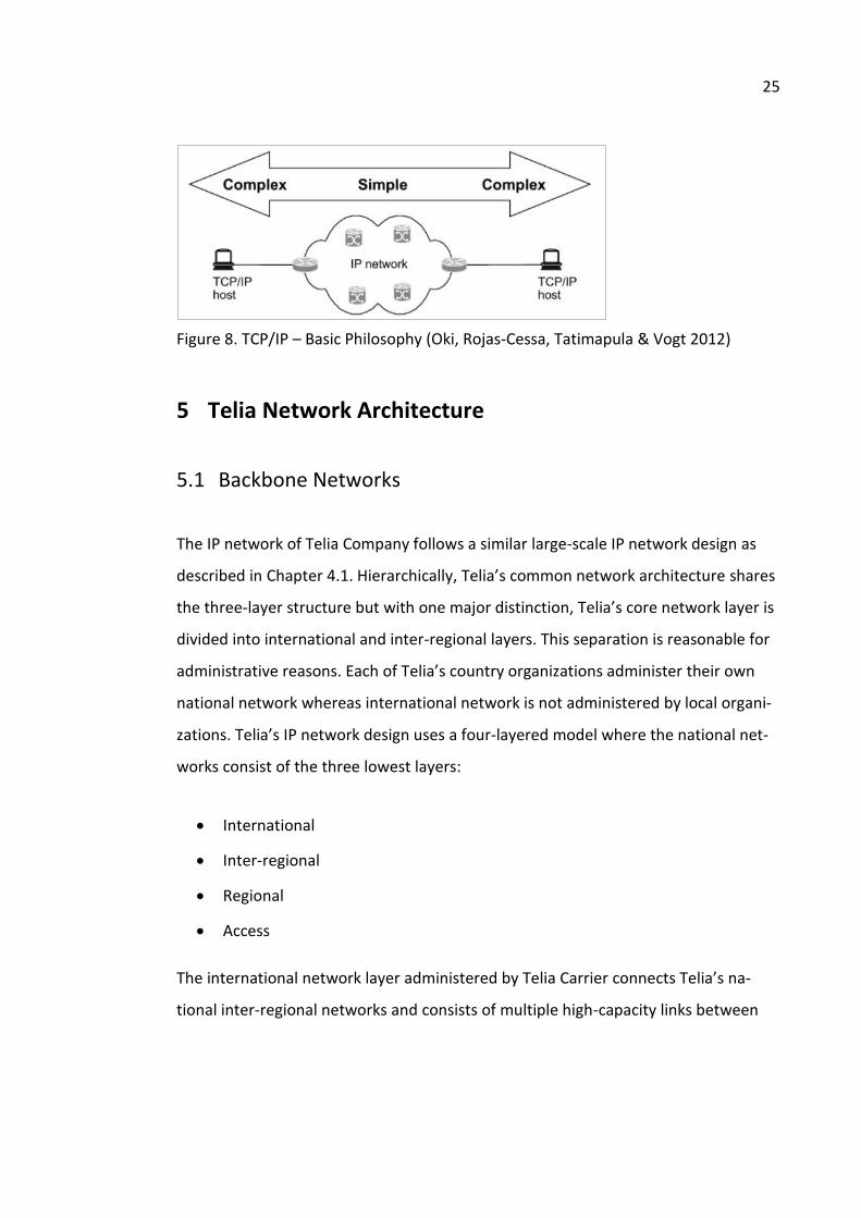
25
Figure 8. TCP/IP – Basic Philosophy (Oki, Rojas-Cessa, Tatimapula & Vogt 2012)
5 Telia Network Architecture
5.1 Backbone Networks
The IP network of Telia Company follows a similar large-scale IP network design as
described in Chapter 4.1. Hierarchically, Telia’s common network architecture shares
the three-layer structure but with one major distinction, Telia’s core network layer is
divided into international and inter-regional layers. This separation is reasonable for
administrative reasons. Each of Telia’s country organizations administer their own
national network whereas international network is not administered by local organi-
zations. Telia’s IP network design uses a four-layered model where the national net-
works consist of the three lowest layers:
International
Inter-regional
Regional
Access
The international network layer administered by Telia Carrier connects Telia’s na-
tional inter-regional networks and consists of multiple high-capacity links between

26
multiple POPs (Point of Presence) around the world. The international backbone net-
work spreads across Europe, Asia and the U.S., forming the second largest ISP back-
bone network of today’s Internet along with other tier 1 ISPs. For reference, a por-
tion of the Telia Carrier’s IP backbone and POPs in Europe can be seen in Figure 9.
Figure 9. International Network (Telia Carrier – Network Map N.d.)
While Telia has only one international network, it has multiple inter-regional net-
works in the Nordic countries. In general, the functions and characteristics of inter-
regional networks are similar to international backbone network and base on IP-
over-WDM MPLS (Multiprotocol Label Switching) backbone, which forwards data in
high speed between long or very long distances. Both of the backbone networks also
rely on diverse capacity links, which connect the core sites as well as provide peering
interconnections with other network providers.
The structure of Telia’s national networks is similar, although network topology var-
ies slightly depending on the country. Figure 10 illustrates Telia’s common principle

27
for inter-regional networks that consist of symmetrical red-blue network halves. In
the figure, ASBR (Autonomous System Border Router) nodes represent peer routers
at the edge of an autonomous system. The other nodes in the figure represent inter-
regional core-level routers connecting regions. Configurations of non-ASBR core rout-
ers are kept simple in order to achieve high-performance traffic forwarding to, for ex-
ample, enable a BGP-free (Border Gateway Protocol) core network.
Figure 10. Inter-regional Network
Although not shown in the figure, the inter-regional networks include infrastructure
support nodes such as DNS (Domain Name System) servers and BGP route reflectors
as well as more ‘intelligent’ service edge routers. The service edge routers collect
consumer and corporate Internet services – and interconnect PSTN (Public Switched
Telephone Network) and mobile networks. As the edge routers are also used as ter-
mination points for customer VPN (Virtual Private Network) services, they are the
first devices participating on the routing from customer’s perspective. Due to dimen-
sions of the countrywide inter-regional networks, Telia’s national networks are fur-
ther composed of several regional network segments that extend reachability within

28
regions. Regional networks collect traffic from large regional areas and aggregate
customer traffic to the inter-regional routers utilizing WDM, OTN (Optical Transport
Network) or fiber connections on a physical layer.
5.2 Regional Network
5.2.1 Topology
There are in total 13 individual regional networks in Finland consisting of Nokia’s ME
(Metro Ethernet) nodes and Huawei’s layer 2 switches. The ME nodes are mainly SR
and ESS series equipment forming the main aggregation ring for the Finnish regional
network. The layer 2 switches are mainly used to backhaul base station traffic as well
as to connect customers but they are not used in the aggregation ring. The list shown
in Table 1 lists the equipment considered as aggregation nodes, which as well are the
device models in the scope of this thesis.
Table 1. Regional Network Nodes Vendor Model Description Type
Nokia
7750 SR-12 Service Router (IP edge) Core/Access
7750 SR-7 Service Router (IP edge) Access
7750 SR-A4 Service Router (IP edge) Access
7750 SR-C4 Service Router (IP edge) Access
7450 ESS-12 Ethernet Service Switch Core/Access
7450 ESS-7 Ethernet Service Switch Access
7210 SAS-X Service Access Switch Access
The ME nodes are categorized into access nodes and core nodes. ME access nodes
are used to aggregate customer traffic using either directly connected customer in-
terfaces or access-to-regional-network interfaces. Unlike the ME access nodes, ME
core nodes do not have directly connected customer subscriptions and their purpose
is to connect to IP core as well as to other ME nodes. Regional networks offer a de-
gree of redundancy with ring-shaped topology, which is the preferred topology.

29
However, usually the physical topology of regional network is actually a combination
of different logical topologies shown in Figure 11.
Figure 11. Logical Topologies (Modified from CCNA 1 and 2 Companion Guide 2005,
62)
Bus topology is considered archaic and is not a suitable for large network due to
scalability issues (CCNA 1 and 2 Companion Guide 2005, 64). Like bus topology, star-
shaped network has a single point of failure, which jeopardizes the network in equip-
ment failure scenarios, and when network congestion occurs. Ring topology, on the
other hand, enables redundancy, because even if a link or an ME node fails, there is
an alternative path towards the backbone network. Although ring-shaped ME node
topology is the basic thought for aggregation networks, in reality, regional networks
are actually mesh networks and may contain parts where ME nodes follow hierar-
chical topology.
A fully connected mesh network offers a high degree of fault tolerance due to maxi-
mum numbers alternate connections. Regardless, a large-scale full mesh network is
expensive to build and maintain as every node is directly connected to every other

30
node. A partially connected mesh network is another type of mesh network, which
provides fault tolerance without requiring the expense of a fully connected mesh
network. In partial mesh topology, nodes connect to only some of the other nodes.
Usually, a typical regional network follows the similar topology as illustrated in Figure
12. The outer rim forms a ring-shaped border for the regional network, but is a par-
tially connected mesh network. In the figure, unlabeled larger grey circles represent
the ME access nodes, which usually have redundant paths towards the red and blue
ME core nodes (MEc). The ME core nodes are directly connected to each other and
provide redundancy towards the IP core and are on the edge of an aggregation area.
The two MEs nodes represent nodes dedicated for supporting the regional network
infrastructure and are not really considered core or access ME nodes. The figure also
includes smaller circles that represent Layer 2 switches which, such as access net-
work nodes, do not have redundant paths towards the inter-regional network.
Figure 12. Regional Network

31
5.2.2 Traffic Forwarding
Routing in regional networks bases on IS-IS (Intermediate System-to-Intermediate
System) IGP (Interior Gateway Protocol), which provides the necessary reachability
information for MPLS (Multiprotocol Label Switching) to form LSPs (Label Switched
Path) within a regional network. The packet forwarding in regions bases on MPLS,
which is common in Carrier Ethernet networks as it provides more efficiency com-
pared to conventional routing of IP packets. According to RFC 3031 (2001, 4) MPLS
reduces IP routing lookups, as packet forwarding does not require the existence of
routing protocols. Instead, it uses MPLS labels that are used to determine the next
hop address of the IP packet. MPLS does not completely remove the IP lookup pro-
cess, as the IP header inspection is done once when packet enters the MPLS network
(RFC 3031 2001, 4).
This first inspection is performed by IS-IS, which uses Dijkstra shortest path algorithm
to calculate best paths through the network. IS-IS is the preferred routing protocol in
large ISP networks because of its ability to scale and because it supports traffic engi-
neering (Carrell et al. 2015). According Unicast Routing Protocols Guide Release
15.1.R1 (2017, 305-306) IS-IS supports large networks by allowing autonomous sys-
tems to be divided into more manageable areas using two-level hierarchy, where
Level 1 routing is performed within a certain IS-IS area separately from Level 2 rout-
ing (intra-area routing) whereas Level 2 routing is performed between IS-IS areas (in-
ter-area routing).
In regional networks, the ME nodes perform Level 1 IS-IS routing. Level 1 routers are
not aware of Level 2 routes and thus must forward traffic to Level 2 IP core routers in
order to reach destinations outside regional networks. MPLS calculates the best
paths using IS-IS metrics, which form the forwarding paths in logically complex large-

32
scale mesh networks. In Figure 13, the green links represent a metropolitan area
near a core site. The orange links represent the connections of ME nodes further in
regional topology, which expand around borders of a region. The metrics shown on
the links ensure that the traffic from the ME access nodes always travels the shortest
path and prevents the traffic looping against the preferred paths. The red dotted ar-
rows represent undesirable paths from ME access nodes towards ME core nodes
whereas the green dotted arrows represent the preferred routes.
Figure 13. IS-IS Areas and Metrics
IP packets forwarded in regional networks are encapsulated within MPLS headers,
which are carried between the data link and network layers. For this reason, MPLS is
considered to operate on layer 2.5. An MPLS header (shown in Figure 14) is only 4
bytes in length, meaning less calculation in the forwarding lookup process, compared
to a 20-byte IP header.

33
Figure 14. Encoding of the MPLS Label Stack (RFC 3032 2001, 3)
In MPLS context, routers that run MPLS are known as LSRs (Label Switching Router).
When a packet arrives into a MPLS domain, it is received initially by an ingress LSR.
Ingress LSR is responsible for handling the incoming traffic by assigning it to a FEC
(Forwarding Equivalence Class), which is used to determine the forwarding proce-
dure of packets. In MPLS networks, all packets assigned to the same FEC are for-
warded in the same manner over the same path. A path, or an LSP in MPLS context,
consists of one or multiple of LSRs capable of forwarding native L3 packets. (RFC
3031 2001, 6-7.)
In Figure 15, PE1 router acts as an ingress LSR and represents a ME access node di-
rectly connected to a CPE. As PE1 receives a plain IP packet, it inspects it and deter-
mines the packet should be forwarded to host H3 through MPLS domain. PE1 then
assigns a FEC for the packet, inserts a MPLS header (label = 1000001) between the IP
and Ethernet headers, and forwards the packet towards P1 via PE1PE4 LSP.

34
Figure 15. LSP Example (Monge & Szarkowicz 2015)
Processing of MPLS-labeled packets is always based on the top label as a single pack-
et can have multiple labels on the MPLS label stack. LSRs participating to MPLS for-
warding may swap the label at the top of the stack (swap), remove a labels (pop) or
add labels into the stack (push) (Monge et al. 2015). In the above figure, P1 performs
a swap action by swapping the label of the MPLS header to 1000002. The packet is
then assigned to the same LSP once again, and as the packet is about to leave the
MPLS domain, egress LSR P2 pops the label and sends the packet towards PE4. As
shown in the example, the forward and return LSPs may be asymmetric.
5.3 Access Network
Most of the services including consumer broadband subscriptions and enterprise
VPN services are connected to access network equipment. Access network layer pro-
vides an extension for regional networks by reaching especially the residential cus-
tomers and the enterprise customers who do not necessarily need high performance

35
services. The access network divides roughly into copper access nodes and fiber ac-
cess nodes.
The fiber access nodes comprise ME nodes, and L2 (Layer 2) switches and optical
FTTH (Fiber to the Home) Ethernet switches providing fiber access for residential cus-
tomers. Although ME nodes and L2 switches are classified as regional nodes, they are
also considered access nodes. The copper access nodes include DSLAMs (Digital Sub-
scriber Line Access Multiplexer), FTTB (Fiber to the Building) Ethernet Switches and
the physical medium determines the access node type for the customers. For CAT 3
customers, DSLAMs are the only available access node type whereas CAT 5/6 cus-
tomers are connected via Fast Ethernet or Gigabit Ethernet interfaces of FTTB
switches.
The copper nodes include also TDMoP (Time Division Multiplexing over Packet)
nodes used to connect mobile base stations, which can be connected using 2048
Mbps E1 Fast Ethernet interfaces. However, for example 4G base stations require
much more capacity than older generation mobile technologies, which is why 4G
base stations use fiber connections. Figure 16 illustrates a MBH (Mobile Backhaul)
connection from a 4G base station towards mobile core network. As shown in the fig-
ure, the MBH is not necessarily forwarded directly to a core router when compared
to conventional customer traffic, which comes from a CPE device through a green ac-
cess node.

36
Figure 16. Service Forwarding and Encapsulation
Appendix 1 describes the interconnection of access and regional networks. The CPE
layer in the appendix is only used to visualize the customer premises and does not
count as a separate network layer in Telia’s network architecture. As illustrated, CPEs
can be directly connected to regional nodes. The appendix features also inter-re-
gional layer, as the ‘regional intelligence’, the service edge routers, reside at core
site’s premises.
6 5G
IMT-2020 (5G) is a next generation mobile network technology, which is currently
being standardized by ITU (International Telecommunications Union) with the help of
other standard development organizations. As of April 2018, ITU has agreed the key
performance requirement of IMT-2020 as well as reached the first-stage approval for
new standards relating closely to upcoming 5G networks (Zhao 2017; Zhao 2018).
Compared to IMT-Advanced (4G), IMT-2020 aims to enhance the existing mobile net-
works by improving the key capability areas shown in Figure 17.

37
Figure 17. Enhancement of Key Capabilities from IMT-Advanced to IMT-2020
(M.2083-0 2015, 14)
Although ITU is the main organization driving the development of IMT-2020, the
other major organization in 5G’s evolution, 3GPP (3rd Generation Partnership Pro-
ject), has been working with a new 5G radio access technology known as NR (New
Radio). In December 2017, 3GPP released initial NR specifications for non-standalone
access, which bases on cooperation of 4G and 5G networks. In the non-standalone
access, both 4G and 5G radios coordinate in the same device to provide necessary
control and data paths for 5G traffic. The first set of NR specifications are capable of
fulfilling many of the IMT-2020’s requirements; however, the standalone access
specifications expected to be ready by the end of the first half of 2018, are required
to fulfill all of the requirements for 5G applications. (Kim et al. 2018.)

38
Because standardization of IMT-2020 is still ongoing, the final architectural models
are not currently known. Still, the device manufacturers have already responded to
the commercialization of 5G networks by introducing solutions for the future 5G ap-
plications. Even though the requirements for 5G networks are tight, not all of the re-
quirements need to be met simultaneously adding flexibility to efficiently support
various 5G applications (Kim et al. 2018). As shown in Figure 18, the 5G applications
are divided into three usage scenarios: eMBB (Enhanced Mobile Broadband), mMTC
(Massive Machine Type Communications) and uRLLC (Ultra-reliable and Low-latency
Communications).
Figure 18. IMT-2020 Usage Scenarios (M.2083-0 2015, 12)
Each of the usage scenarios require distinct key capability parameters from IP net-
works. For example, eMBB applications have high importance in area traffic capacity,
peak data rate, user experienced data rate and spectrum efficiency. On the other
hand, mMTC applications do not depend so much on these parameters. Instead, the

39
most important parameter is connection density to support the tremendous num-
bers of devices, which may transmit data only occasionally. In high mobility uRLLC ap-
plications, low latency and high mobility are the most essential parameter to secure
e.g. transportation safety of autonomous vehicles. (M.2083-0 2015, 15.)
7 Network Performance
7.1 Metrics
The overall network performance is a combination of factors affecting both packets
and frames when they are transmitted over networks. As communication networks
operate on different TCP/IP layers, the performance metrics for network and data-
link layers have been specified by different organizations: MEF (Metro Ethernet Fo-
rum) and ITU’s Telecommunication Standardization Sector. As this thesis focuses on
measuring L3 latency, Chapter 7 neither covers the L2 metrics defined by MEF nor
provides a comprehensive theory about all L3 metrics.
In IP networks, packet forwarding decisions are based on the most current network
conditions. The paths to the other networks constantly change due to hardware fail-
ures or excessive use of network’s available capacity. This, in addition to the fact that
there are no performance monitoring authorities for the Internet, makes IP networks
generally unreliable. Hence, performance monitoring is a responsibility that falls to
the individual service providers. (Carrell et. al 2015.)
In many cases, today’s IP network design requires that packets make several hops
before reaching their destination. Each of the hops represents a point in the net-
work, which can make packet susceptible to performance issues. In some cases, per-
formance issues may result from a single cause, e.g. equipment failure or congestion,

40
however, in some cases poor network performance does not have a single cause.
(Carrell et al. 2015.) According to Carrell et al. (2015), the common network perfor-
mance is composed of the following metrics:
Latency measures how long it takes a PDU (Protocol Data Unit) to travel from node to another. Latency can either be measured as one-way (source to desti-nation) or two-way (round-trip time) latency.
Packet/Frame Loss indicates the number or percent of PDUs that do not reach their intended destination.
Retransmission of a PDU occurs when packet is lost and a reliable transport protocols (e.g. TCP) is used for transmission. Retransmission delay measures the amount of time required to retransmit the PDU lost PDU.
Throughput is a measure of amount of traffic a network can handle.
In addition to above metrics, several other performance metrics exist. ITU’s recom-
mendation Y.1540 defines more comprehensive metrics for measuring IP packet
transfer and availability performance. According to Y.1540 (2016, 16-28), additional
IP performance parameters include: IP service availability, end-to-end 2-point IP
packet delay variation, spurious IP packet rate and several capacity metrics as well as
ratios for IP packet errors and reordered packets.
Regarding 5G, the latest requirements for performance metrics of some applications
can be seen in Appendix 2 (3GPP TS 23.501 v15.0.0 2017, 89). The 3GPP’s QoS model
shown in the Appendix defines packet error rate and packet delay budget for 5G ap-
plications. However, the QoS model does not yet contain latency requirements for all
5G applications.

41
7.2 Network Delay
Latency – or network delay indicates how much time it takes for a datagram to get
transmitted from one point to another. To the most of us, network delay of modern
IP network is probably most noticeable and concrete, when we are on a voice over IP
call with a person in the same room. It might be thought that delay is not, in fact,
much of an issue in people’s everyday life. However, when there is a need to imple-
ment new latency critical applications such as more advanced industrial automation
or intelligent transport systems, delay becomes a much more critical metric. Accord-
ing to Evans & Filsfils (2007, 4), time-critical applications are highly dependent on low
latency, which is why SLA (Service Level Agreement) terms for network delay are de-
fined for one-way delay. On the contrary, for more adaptive TCP applications it is
more reasonable to define SLA terms for two-way delay (Evans et al. 2007, 4).
Network delay can be measured as one-way delay and two-way delay. Measuring
one-way delay over two-way delay is more accurate, since measuring round-trip de-
lay measures the performance of two distinguished network paths together. Hence,
the network paths in IP networks are considered asymmetric, which means that the
actual physical path from a source to the destination may differ from the path from
the destination to the source. The delay of the forward and reverse path may also be
asymmetric due to asymmetric queuing or because paths’ QoS provisioning may dif-
fer in both directions. Finally, applications do generate unequal amount of data for
both directions, which can make an application more dependent on the performance
in one direction. (RFC 2679, 2-3.)
Both one-way and two-delay are caused by the various delay components. First of all,
serialization delay (also known as transmission delay) occurs when a packet is sent
into the transmission media. Serialization delay depends on packet size and link

42
speed and is proportional to packet size and inversely proportional to link speed (Ev-
ans et al. 2007, 6-7):
𝐷𝑠𝑒𝑟𝑖𝑎𝑙𝑖𝑧𝑎𝑡𝑖𝑜𝑛 =𝑏𝑖𝑡𝑠
𝑠𝑙𝑖𝑛𝑘
where bits = transmitted bits and slink = link speed
Serialization delay is not significant in regional IP networks since the ME nodes are
connected together with high-speed transmission links. The next delay component is
equal to the time taken for a bit to reach destination is constrained by the distance
and the physical media (Evans et al. 2007, 5). Propagation delay is constrained by the
speed of light in the transmission medium and depends upon the distance. In optical
fibers, the theoretical maximum travel speed of is only near to the speed of light c
due to refractive index of fibers’ glass core (Miller 2012). For reference, propagation
delay increases when electric medium such as copper cable is used. Then maximum
travel speed of the electric signal is roughly ⅔ of the constant c.
𝐷𝑝𝑟𝑜𝑝𝑎𝑔𝑎𝑡𝑖𝑜𝑛 =𝑑
𝑠
where d = distance and s = wave propagation speed
Because physical laws constrain the propagation speed, the only way on controlling
propagation delay is control the physical link routing or alternatively, change the net-
work topology to reduce the propagation delay (Evans et al. 2007, 5-6). The propaga-
tion delay is the most noticeable in very long distances, even if the best available
transmission technology is used. This can be seen in Table 2, which contains Telia
Carrier’s round-trip statistics about packet loss ratios and packet delay.

43
Table 2. Telia Carrier’s Performance Report – March 2018 (Telia Carrier – Services)
Routers also need to time to process the IP packets, which causes another delay
component, switching delay. The switching delay is the time difference between host
receiving a packet on ingress interface and transmitting the packet into the medium.
Typically, switching delays are 10-20 microseconds in hardware-based switching and
more if software-based router implementations are used. If the distances between
routers or switches are long, switching delays are insignificant compared to the over-
all end-to-end delay. Lastly, if a router receives more packets to its ingress interfaces
that it is able to process, the packets are queued. This adds another factor (schedul-
ing or queuing delay) to overall delay since packets must remain in the queue until
forwarding conditions defined by the scheduling algorithm are met. (Evans et al.
2007, 6.) Finally, the end-to-end delay is the sum of all of the delay components (Ev-
ans et al. 2007, 5):
𝐷𝑡𝑜𝑡 = (𝐷𝑠𝑒𝑟 + 𝐷𝑝𝑟𝑜 + 𝐷𝑠𝑤𝑖 + 𝐷𝑠𝑐ℎ)

44
where Dtot = total delay, Dser = serialization delay, Dpro = propagation delay, Dswi =
switching delay and Dsch = scheduling delay
According to Y.1540 (2016, 17), IPTD (IP packet Transfer Delay) is defined for all suc-
cessful and errored packet outcomes across a basic section or a Network Section En-
semble (NSE). IPTD (shown in Figure 19) is calculated using ingress and egress event
IPREs (Internet Protocol packet transfer reference event):
IPTD is the time, (t2 – t1) between the occurrence of two corresponding IP packet reference events, ingress event IPRE1 at time t1 and egress event IPRE2 at time t2, where (t2 > t1) and (t2 – t1) ≤ Tmax. If the packet is fragmented within the NSE, t2 is the time of the final corre-sponding egress event. (Y.1540 2016, 17.)
Figure 19. End-to-end Transfer of an IP Packet (Y.1540 2016, 17)
In the figure, the one-way end-to-end IPTD is the delay between the measurement
point (MP) at the source (SRC) and destination (DST). ELs represent exchange links con-
necting hosts (source/destination host and routers) whereas NSs represent a set of hosts
and links that together provide IP service between the source and destination host.

45
Y.1540 also defines mean, minimum and median metrics for end-to-end IPTD. Mean
IPTD is the arithmetic average of IP packet transfer delays. Minimum IPTD is the
smallest value of IPTD among all IP packet transfer delays and includes propagation
delay and queuing delays common to all packets. Therefore, minimum IPTD may not
represent the theoretical minimum delay of the path between measurement points.
Median IPTD is the 50th percentile of the frequency distribution of IP packet transfer
delays representing the middle value once the transfer delays have been rank-or-
dered. (Y.1540 2016, 18.)
7.3 Delay Variation
Delay variation is an important metric to some of the applications. For example,
streaming applications may use information about the total range of IP delay varia-
tion to avoid buffer underflow and overflow. Extreme variation of IP delay will also
cause problem TCP connections as TCP’s retransmission timer thresholds grow and
may cause delayed packet transmission or even unnecessary transmissions. (Y.1540
2016, 18.)
Delay variation (also referred to as jitter) may be a result of several occurrences. If
the network topology changes because of a link failure or because LSPs change, the
change in propagation delay may cause a sudden peak in delay variation. For the
same reason, if the traffic is rerouted over links with slower speeds, serialization may
contribute to jitter. Variation in scheduling delay may cause delay variation if sched-
uler buffers oscillate between empty and full. In addition, switching delay may affect
jitter, however, since modern routers use hardware-based packet switching, the
switching delay variation is a lesser consideration. (Evans et al. 2007, 8.)

46
End-to-end 2-point IP packet delay variation bases on the measured delay for consec-
utive packets and is measured observing IP packet arrivals at ingress and egress
measurement points (Y.1540 2016, 18). According to Evans et al. (2007, 8), it is fun-
damental that delay variation is measured as one way delay since measuring round-
trip delay is not sensible. IP delay variation is calculated as presented in Figure 20.
Figure 20. End-to-end 2-Point IP Packet Delay (Y.1540 2016, 19)
8 Performance Monitoring Methods
8.1 Overview
In general, network performance monitoring methods can be considered as either
active or passive. Active methods generate synthetic packet streams whereas passive
methods base on observation of unmodified (real) traffic. Passive methods base

47
most importantly on the integrity of the measured traffic flow; meaning that passive
method must not generate, modify or discard packets in the test stream (RFC 7799
2016, 5). Other attributes of active methods include that:
The packets in the stream of interest have (or are modified to have) dedicated fields or field values for measurement
The source and destination measurement points are usually known in advance
The characteristics of the packet stream of interest are known by the source
(RFC 7799 2016, 4.)
The important characteristic of a passive method is that it relies solely on observa-
tion of packet steams. Unlike active methods, passive methods does not influence
the quantities measured, which removes the need to analyze and/or minimize ef-
fects of synthetic test traffic. However, passive methods collect information using a
collector, which may increase traffic load when transferring measurement results to
collector. Passive methods depend on existence of one or more packets streams and
require often more than one designated measurement point. If more than one meas-
urement point is used to e.g. measure the latency between two measurement
points, passive methods require that packets contain enough information determine
the results. (RFC 7799 2016, 5.)
Some methods may use a subset of both active and passive attributes making them
hybrid methods. RFC 7799 defines two hybrid categories: Hybrid Type I and Hybrid
Type II. Hybrid Type I is a synthesis of the fundamental methods (active and passive),
which focuses on single packet stream. An example of a Hybrid Type I method, is a
method that generates synthetic stream(s) and observes an existing stream accord-
ing to the criteria for passive methods. Hybrid Type II methods employ two or more
different streams of interest with some degree of mutual coordination (e.g. one or
more synthetic packet streams and one or more undisturbed and unmodified packet

48
streams) to enable enhanced characterization from additional joint analysis. (RFC
7799 2016, 6-7.)
The two methods, ping and TWAMP, used in this study are examples of purely active
methods. Passive measurement protocols such as SNMP (Simple Network Manage-
ment Protocol) collects and stores a great amount of data, which is not necessary (or
even reasonable) to conduct simple end-to-end measurements. Active methods on
the other hand provide a more efficient way of gathering specific data from network
elements.
8.2 Ping
8.2.1 Basic Operation
The best-known example of an active method of measurement is ping utility. Ping
provides a simple method to test network host reachability as well as is able to re-
port diagnostic reports about errors, packet loss and round-trip times. Ping operates
on layer 3 and uses an echo query-and-response ICMP (Internet Control Message
Protocol) messages. According to Huston (2003), the basic operation of ping is sim-
ple: a ping source generates an ICMP echo message and sends it to a destination
host. The destination receiving the IP packet then examines the ICMP header, forms
an ICMP echo request message based on ICMP echo message and sends it back to
the ping source. This operation is described in Figure 21.

49
Figure 21. ICMP Echo Query and Response (Hundley 2009, 253)
Ping implementations and the parameters supported vary among different operating
systems. Usually ping programs allow modifying parameters such as send interval
and number of sent echo requests or changing TTL (Time to Live), TOS (Type of Ser-
vice) and source address of the host by setting IP header fields. Typically, ping pro-
grams also allow set the amount of padding that should be added to the packet. De-
pending on the ping program and operating system, also other parameters can be
set. The example output shown below displays a summary of loss and round-trip de-
lay statistics (minimum, maximum and standard deviation) for the five sent packets
when ping command was issued on SR OS (Service Router Operating System) device.
*A:vSim1# ping <IP address> rapid size 1024 pattern 65532 do-not-fragment PING <IP address> 1024 data bytes !!!!! ---- <IP address> PING Statistics ---- 5 packets transmitted, 5 packets received, 0.00% packet loss round-trip min = 1.21ms, avg = 1.36ms, max = 1.41ms, stddev = 0.076ms
ICMP messages use IP protocol number 1 and are constructed at the IP layer. The
messages encapsulated within IP packets are considered part of the IP layer itself,
and like UDP, ICMP does not guarantee delivery. A ping might also result in a destina-
tion unreachable ICMP-message, which can indicate that packet might not have a
route between the hosts or then it might have been discarded. (Hundley 2009, 252-
253.)

50
Ping uses the header format shown in Figure 22 for generating both ICMP echo and
ICMP echo replies between network hosts. The three first fields are common to all
ICMP messages: an 8-bit type and code followed by a 16-bit checksum. (Goralski
2017).
Figure 22. ICMP Echo/Reply Header (RFC 792 1981, 14)
The type field defines the purpose of the ICMP message. According to Goralski
(2017), type field is used to recognize about 40 different ICMP message types catego-
rized in two major categories: error messages and queries. The Table 3 shows some
of the non-optional ICMP message types that are mandatory to implement in net-
work hosts. Note that ICMP messages also include optional messages types, which
are not presented in Table 3.
Table 3. ICMP Message Types (Modified from Goralski 2017) Type Meaning Codes Catogory
0 Echo Reply 0 Query
3 Destination Unreachable 0-15 Error
5 Redirect 0-3 Error
8 Echo Request 0 Query
11 Time Exceeded 0-1 Error
12 Parameter Problem 0-2 Error
17 Mask Request 0 Error
18 Mask Reply 0 Error
37 Domain Name Request 0 Error
38 Domain Name Reply 0 Error
The code gives additional information about the condition of the message type and
usually most of the ICMP messages use only Code=0. The checksum is equivalent to
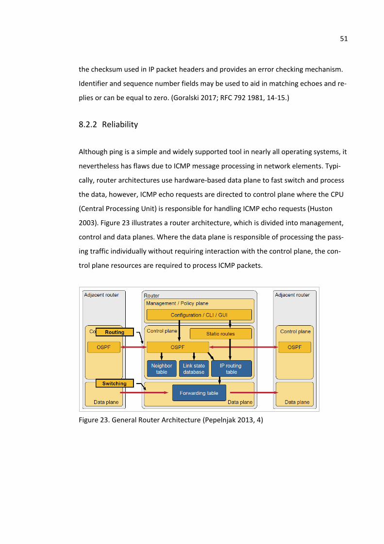
51
the checksum used in IP packet headers and provides an error checking mechanism.
Identifier and sequence number fields may be used to aid in matching echoes and re-
plies or can be equal to zero. (Goralski 2017; RFC 792 1981, 14-15.)
8.2.2 Reliability
Although ping is a simple and widely supported tool in nearly all operating systems, it
nevertheless has flaws due to ICMP message processing in network elements. Typi-
cally, router architectures use hardware-based data plane to fast switch and process
the data, however, ICMP echo requests are directed to control plane where the CPU
(Central Processing Unit) is responsible for handling ICMP echo requests (Huston
2003). Figure 23 illustrates a router architecture, which is divided into management,
control and data planes. Where the data plane is responsible of processing the pass-
ing traffic individually without requiring interaction with the control plane, the con-
trol plane resources are required to process ICMP packets.
Figure 23. General Router Architecture (Pepelnjak 2013, 4)

52
For example in Juniper router architecture, the data plane also limit rates how many
ICMP echo requests are passed to the control plane. Furthermore, processing of
ICMP messages is considered a low-priority task meaning the router is not ready to
respond until it has finished processing higher-priority tasks such as building the
routing table. (Marschke, Reynolds & Southwick 2011, 473.)
Due to ICMP echo requests are processed at a lower priority makes ping unreliable
method of determining the actual performance of network paths. Ping also relies on
round-trip measurements, which gives an approximate value of the one way-delay.
By measuring the round-trip delay, the one-way delay may or may not be roughly
half of the round-trip delay, because ICMP echo and ICMP reply packets do not nec-
essarily return the same path. As mentioned in earlier chapters, QoS markings in two
directions may also be asymmetric, which results in an unequal amount queuing time
the test packet spends in the scheduler. However, routers are supposed to set the
TOS field (precedence) of an IP packet to 6 or 7 giving it a high priority to secure its
delivery to the destination address (Goralski 2017). Regardless, this does not priori-
tize ICMP packets at the control plane and only gives them higher priority as they are
passed from router to another.
Ping is generally considered a not reliable method of measuring the network perfor-
mance. Some vendors even discourage using ping to measure latency as ICMP pro-
cessing delay with certain equipment can be up to four milliseconds or more
(KB27335 N.d.). Consequently, TWAMP is becoming more preferable method for
measuring latency, which advantages are listed in Table 4.

53
Table 4. Comparison of TWAMP and Ping (TWAMP Explained 2014)
8.3 TWAMP
8.3.1 Overview
TWAMP is a protocol used to measure the metrics of bidirectional IP performance
between two devices. It uses the OWAMP (One-Way Active Measurement Protocol)
architecture initially developed for measuring only unidirectional metrics such as
one-way delay or packet loss in IP networks. Because TWAMP bases on OWAMP, it is
capable of measuring also one-way metrics, which however, is less common in IP
networks. Two-way measurements are primarily used as remote measurement point
may be limited to a simple echo function, and because round-trip metrics does not
require synchronization between local and remote measurement points. (RFC 5357
2008, 1-2.)
Compared to ping, TWAMP is a less familiar measurement method. There are not
many publicly available research results or publications concerning TWAMP and

54
probably the most informative research for comparison of ping and TWAMP is dis-
cussed in Ingmar Bäckström’s master’s (2009) thesis. In his thesis, Bäckström imple-
mented a measurement topology where two test probes were connected over an In-
ternet connection. The test sessions between the probes were conducted with
TWAMP, ping as well as two other active measurement methods.
According to Bäckström (2009, 29), ping performed well compared to TWAMP, as
there was no significant difference in two-way latency in the test sessions. The aver-
age round-trip delay of ping test session was around 1 millisecond more than round-
trip delay compared to TWAMP when three separate test sessions were conducted.
In the three test sessions, the ping measurements resulted in a 0.3% to 3.4% greater
round trip delay. However, in one of the tests, the dispersion of ping’s round-trip de-
lays was worse than measured with TWAMP.
TWAMP consists of four logical entities: the Control-Client, the Session-Sender, the
Server and the Session-Reflector (RFC 5357 2008, 4). Like ping, TWAMP uses echo/re-
ply principle where Session-Reflector employs time stamps and reflects test packets
back to the source (Session-Sender) over a TWAMP-test session. Figure 24 illustrates
to logical model of TWAMP where the roles have the following definitions:
Session-Sender The sending endpoint of an TWAMP-Test session
Session-Reflector The receiving endpoint of an TWAMP-Test session which is able the reflect packets but does not collect packet information
Server An end system that controls TWAMP-Test sessions and is capable configuring of per-session state in the endpoints
Control-Client A system that initiates and/or terminates TWAMP-Test sessions
(RFC 4656 2006, 4; RFC 5357 2008, 3-4.)

55
Figure 24. Logical Structure of TWAMP (RFC 5357 2008, 4)
As shown in Figure 24, each of the logical roles can be implemented to different
hosts. This adds more freedom for device manufacturers to decide which roles
should be assigned to TWAMP hosts. According to RFC 5357 (2008, 3) typical TWAMP
measurement architecture (shown in Figure 25) usually uses only two hosts which al-
lows protocol simplifications compared to OWAMP. In two-host TWAMP implemen-
tation the host responsible of the Control-Client and Session-Sender roles, is referred
to as the controller; and the host responsible of the Server and Session-Reflector
roles is the responder.
Figure 25. Roles of the TWAMP Hosts (RFC 5357 2008, 4)

56
Despite the fact that TWAMP hosts have been originally named as the controller and
the responder in the TWAMP standard, vendors have adopted a slightly more com-
mon naming convention. Generally, the TWAMP hosts form a client-server model. A
TWAMP ‘client’ is a host containing the Control-Client and Session-Sender role and a
host containing the Server and/or Session-Reflector role is referred to as ‘server’. Re-
gardless, TWAMP implementations are vendor-specific.
Where Cisco and Nokia use similar two-host model than defined in the RFC 5357, Ju-
niper TWAMP client does not require that the Server and the Session-Reflector are
implemented on the same physical device. Hence, Juniper TWAMP clients operate
with a 3rd party server implementations. (7450 ESS, 7750 SR, 7950 XRS, and VSR OAM
and Diagnostics Guide R15.1.R1 2017, 270; IP SLAs Configuration Guide, Cisco IOS XE
Release 3S 2018; Understanding Two-Way Active Measurement Protocol on Routers
2018.)
8.3.2 TWAMP-Control
TWAMP measurement session consists of two inter-related protocols, which both
have specific tasks. TWAMP-Control is used to initiate, start and control measure-
ment sessions, whereas TWAMP-Test is responsible for transmitting test packets be-
tween two TWAMP entities. Before TWAMP measurements can be performed, a se-
ries of tasks have to be accomplished during the TWAMP-Control connection setup.
(RFC 5357 2008, 3.)
A TWAMP session is initiated by the Control-Client when it establishes a TCP connec-
tion with the Server on port 862. Next, the Server responds using a greeting message
indicating the available security modes and other parameters presented in Figure 26
for the connection. (RFC 4656 2006, 6-7; RFC 5357 2008, 6.)

57
Figure 26. Server-Greeting Message (RFC 4656 2006, 7)
TWAMP supports the following authentication modes: 1 for unauthenticated, 2 for
authenticated and 4 for encrypted and 8 for mixed mode (RFC 5618 2008, 4). If the
Control-Client receives a greeting message which modes field is equal to zero, server
indicates that it is not willing to proceed with the control setup. Otherwise, the Con-
trol-Client must send a Set-Up-Response message show in Figure 27 used to inform
about the chosen parameters. (RFC 4656 2006, 8.) Other parameters in the Server-
Greeting message include:
Challenge A random sequence of octets generated by the server; challenge is used to prove posession of shared secret
Salt A pseudo-randomly generated binary string
Count A value of power of 2 which is at least 1024
MBZ (Must be Zero)

58
Figure 27. Set-Up-Response Message (RFC 4656 2006, 8)
In Set-Up-Response message, Mode represents the mode that the client chooses to
use during TWAMP-Control session. The client may also set Mode bits to zero to indi-
cate that it will not continue with the session, which triggers a TCP session closure by
the server. KeyID, Token and Client-IV fields are left unused, if unauthenticated mode
is selected. Otherwise, the Control-Client forms the following: a KeyID containing the
shared secret the client wishes to use for authentication or encryption, a token con-
taining an encrypted concatenation of a 16-octet Challenge, a randomly generated
AES (Advanced Encyption Standard) session key used for encryption and 32-octet
HMAC-SHA1 session key for authentication. (RFC 4656 2006, 8-9.) If the server is
ready to progress establishing TWAMP-Control, it responds with Server-Start mes-
sage shown in Figure 28, which concludes the TWAMP-Control connection setup. The
Server-Start message includes fields for the following parameters:
Accept Value representing server’s willigness to communicate with the client
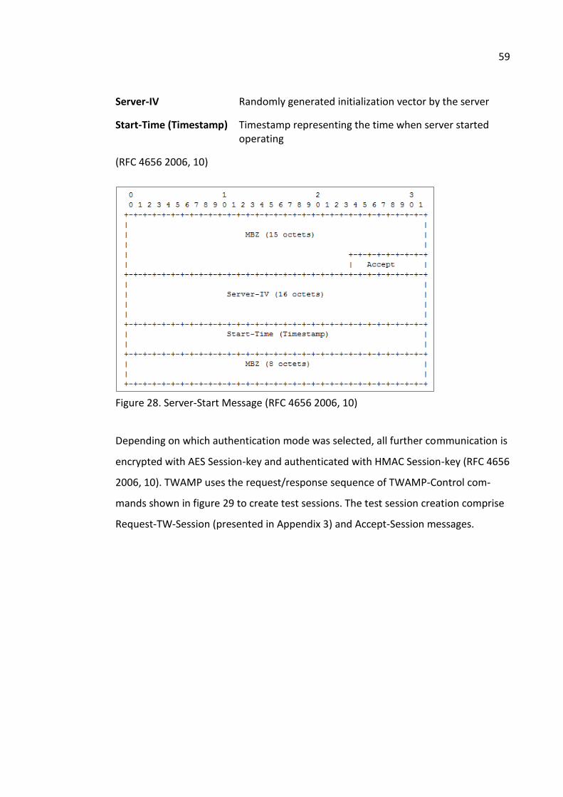
59
Server-IV Randomly generated initialization vector by the server
Start-Time (Timestamp) Timestamp representing the time when server started operating
(RFC 4656 2006, 10)
Figure 28. Server-Start Message (RFC 4656 2006, 10)
Depending on which authentication mode was selected, all further communication is
encrypted with AES Session-key and authenticated with HMAC Session-key (RFC 4656
2006, 10). TWAMP uses the request/response sequence of TWAMP-Control com-
mands shown in figure 29 to create test sessions. The test session creation comprise
Request-TW-Session (presented in Appendix 3) and Accept-Session messages.

60
Figure 29. TWAMP-Control Commands (Modified from RFC 4656 2006, 13-21; RFC
5357 2008, 7-10)
By sending a Request-TW-Session, the Control-Client sends parameters such as IP
version, sender and receiver IP addresses as well as port numbers. Unlike OWAMP,
TWAMP does not use Number of Schedule Slots field indicating when exactly
TWAMP sends the test packets, and additionally does not need to communicate the
amount of test packet beforehand to the server. (RFC 4656 2006, 15-16; RFC 5357
2008, 9.) The other parameters in Request-TW-Session message header are:
SID Test session identifier
Padding Length Amount of padding to append a TWAMP test packet
Start Time Timestamp indicating the session start time
Timeout Timestamp for session timeout
Type-P Descriptor Field for setting traffic class
(RFC 4656 2006, 16-17.)
After receiving Request-TW-Sessions message, the server responds with Accept-Ses-
sion message (presented in Figure 30), indicating either rejection or acceptance for
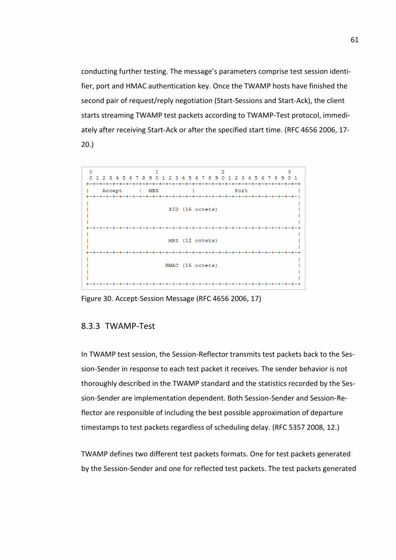
61
conducting further testing. The message’s parameters comprise test session identi-
fier, port and HMAC authentication key. Once the TWAMP hosts have finished the
second pair of request/reply negotiation (Start-Sessions and Start-Ack), the client
starts streaming TWAMP test packets according to TWAMP-Test protocol, immedi-
ately after receiving Start-Ack or after the specified start time. (RFC 4656 2006, 17-
20.)
Figure 30. Accept-Session Message (RFC 4656 2006, 17)
8.3.3 TWAMP-Test
In TWAMP test session, the Session-Reflector transmits test packets back to the Ses-
sion-Sender in response to each test packet it receives. The sender behavior is not
thoroughly described in the TWAMP standard and the statistics recorded by the Ses-
sion-Sender are implementation dependent. Both Session-Sender and Session-Re-
flector are responsible of including the best possible approximation of departure
timestamps to test packets regardless of scheduling delay. (RFC 5357 2008, 12.)
TWAMP defines two different test packets formats. One for test packets generated
by the Session-Sender and one for reflected test packets. The test packets generated

62
by the Session-Sender are UDP traffic and the format depends on which authentica-
tion mode was selected in during TWAMP-Control protocol phase. A TWAMP test
packet sent by the Session-Sender contains the fields shown in Figure 31. (RFC 4656
2006, 29-31; RFC 5357 2008, 12.)
Figure 31. TWAMP Test Packet Format I (RFC 4656 2006, 30)
The above figure represents the packet format when authenticated or encrypted
mode is in use. When TWAMP is used in unauthenticated mode no Must Be Zero nor
HMAC fields are used in the test packets. Regardless of the mode, TWAMP uses the
Sequence Number field to track subsequent test packets, as well as timestamp field,
which divides into two sections 32-byte section containing integers and fractions of
seconds. The header also includes a 16-byte field including an error estimate and in-
formation if TWAMP host generating the test packet, is synchronized to an external
NTP (Network Time Protocol) source. (RFC 4656 2006, 29-31.)

63
The Session-Reflector must send a response to each TWAMP test packet sent by the
Session-Sender as immediately as possible by performing the following actions (RFC
5357 2008, 13-14):
Timestamp the received packet
Decrypt and/or check the integrity of the packet if authenticated or en-crypted mode was used
Copy the sequence number into to the corresponding reflected packet
Fetch the TTL field value from the IP header and replace the value set by the Session-Sender
Ignore packet after timeout (following the Stop-Sessions command)
TWAMP-Test packet format depends on the selected mode. If unauthenticated mode
was selected the test packet format sent by session reflector is similar than show in
Figure 32. A reflected test packet contains a sequence number, a timestamp and an
error estimate generated independently from arriving test packets. Reflector is also
responsible of copying sender sequence number, timestamp and error estimate from
the received packet; as well as copying the TTL value from IP header to Sender TTL
field. In order to compensate reflectors larger packet format, the sender must ap-
pend the test header size by at least 27 or 56 octets depending of the mode. There-
fore, the reflector should reduce sufficient amount of packet padding to achieve
equal payload size. (RFC 5357 2008, 13 and 17-18.)

64
Figure 32. TWAMP Test Packet Format II (RFC 5357 2008, 15)
The TWAMP test session continues as long as the session-sender receives a Stop-Ses-
sions message from the Control-Client. The Server may also close the TWAMP sus-
pend any control connections if no associated test packets have been received and
SERVWAIT or REFWAIT timeout value has been configured. (RFC 5357 2008, 6.)
8.3.4 TWAMP Light
Whereas there are not many publications or research regarding TWAMP, there are
even less for TWAMP Light. TWAMP Light, briefly described in Appendix I of RFC
5357, is an optional model for responders. It allows responders to act as light test
points in the network using TWAMP packet format to gather IP delay, jitter and loss
statistics. The Appendix I in RFC 5357 provides only general overview of TWAMP
Light protocol, which is presented in Figure 33.

65
Figure 33. TWAMP Light: Controller and Responder Roles (RFC 5357 2008, 23)
The most distinguishable difference in TWAMP Light implementation is that the
Server role has been moved from the responder to the controller. This means that
the controller establishes the test session with the server using non-standard means.
Although the responder follows the standard Session-Reflector behavior as described
earlier, there is an exception: the responder does not need to have knowledge of the
session state. In this case, the Session-Reflector must copy the Sequence Number of
the received packet to the Sequence Number field of the reflected packet. (RFC 5357
2008, 23.)
Consequently, these differences eliminates the need for the TWAMP-Control Proto-
col, however, using a non-standard session establishment the following security fea-
tures should be considered:
The non-standard Responder Control Protocol should use an authentication mode and should have means to accept only authenticated and encrypted modes of TWAMP-Test protocol.
The Responder should be configurable to accept only authenticated control sessions.
The Session-Reflector must have a mechanism for key generation.
(RFC 5357, 23-24.)

66
9 TWAMP Implementation
9.1 TWAMP Light
9.1.1 Preparation
The first preliminary steps before implementing TWAMP were to find out the specifi-
cations of the laboratory equipment and if there were in use and if there were any
differences regarding TWAMP or TWAMP Light. Examination of Nokia’s OAM (Opera-
tion Administration and Maintenance) and Diagnostics Guides revealed that TWAMP
was first introduced for SR OS in March 2011 with 9.0.R1 software release. Interest-
ingly, the newest version of SR OS offered exactly the same configuration options for
TWAMP than the 9.0.R1. Another finding was that there were no references to
TWAMP Light protocol until the release of 12.0.R4 OAM and Diagnostics Guide.
All testing relating to TWAMP and TWAMP Light were conducted in Telia’s laboratory
environment, which consisted of Nokia’s VSRs (Virtual Service Router) and physical
SRs (Service Router). At first, the initial tests were restricted to VSRs as the environ-
ment was not familiar and there were other ongoing tests. In the beginning, the only
thing that was known about VSRs was that they in fact were virtualized SR series
routers run on the same CentOS host machine. In practice, this meant that VSR to-
pology (as well as the other configuration) had to be charted by logging directly to
the CLI (Command Line Interface) of the devices. The VSRs followed a ring-shaped to-
pology using VLAN (Virtual Local Area Network) tagged point-to-point links as shown
in Figure 34. In the figure, the dotted blue line represents the interface of CentOS
host, which connects vSim1 router to physical 7450 ESS7 service switch. Note that all
IP addresses and most of the device names have been masked or hidden in figures
and configuration examples presented in the following chapters.

67
Figure 34. VSR Topology
All of the VSRs shared the same SR OS software version TiMOS-B-12.0.R8 and simu-
lated the same 7750 SR-12 chassis model. By default, all Nokia’s SR and ESS series
equipment are connected with SNMP to 5620 SAM (Service Aware Manager) man-
agement client, which is used to gather statistics from the equipment as well as used
as a configuration client. However, the VSRs were not connected to Nokia’s 5620
SAM due to MTU (Maximum Transmission Unit) issues in the physical network inter-
face card of the CentOS host machine.
9.1.2 MPLS and BGP
TWAMP Light configuration was started by configuring a VPRN (Virtual Private
Routed Network) service, as VPRN-based TWAMP Light session was the only example
in Nokia’s configuration guides (Note: It was later found out that TWAMP Light ses-
sion does not necessarily need a VPRN service). A VPRN is Nokia’s term for a L3VPN
service, which connects PE (Provider Edge) routers over a service providers MPLS
backbone. In VPRN, the PE routers associated to a specific VPRN service also need to
share routes using a Multiprotocol BGP.
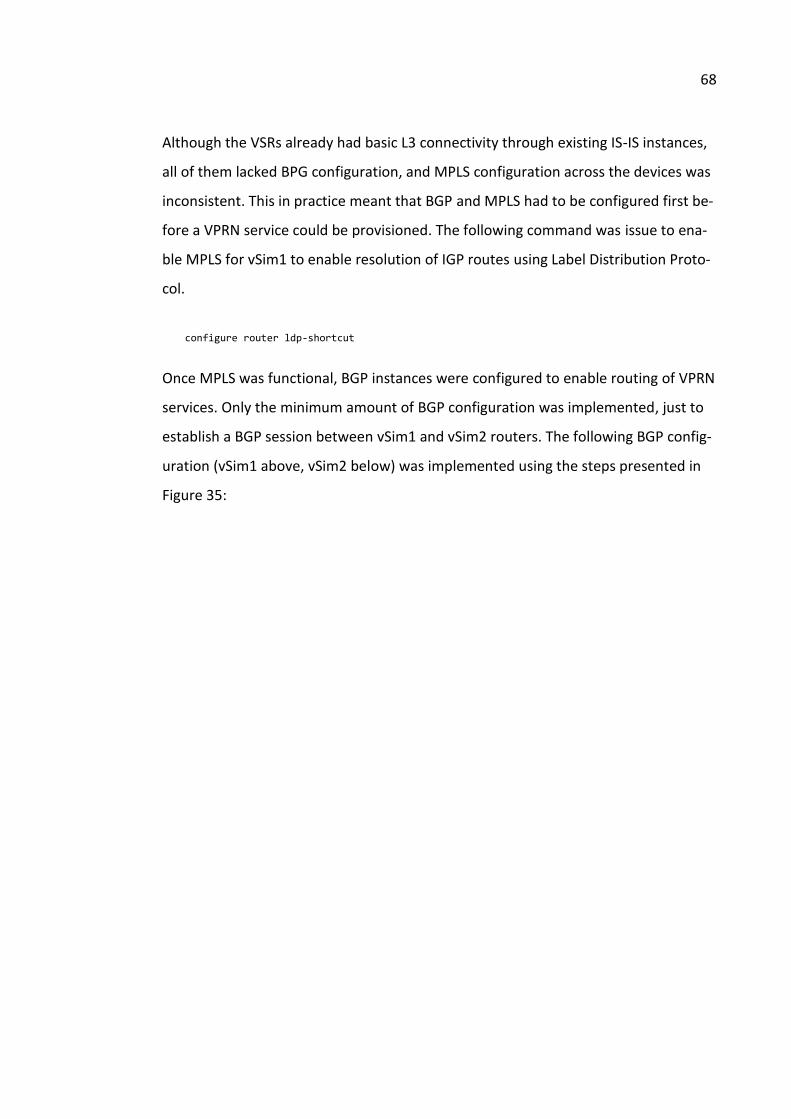
68
Although the VSRs already had basic L3 connectivity through existing IS-IS instances,
all of them lacked BPG configuration, and MPLS configuration across the devices was
inconsistent. This in practice meant that BGP and MPLS had to be configured first be-
fore a VPRN service could be provisioned. The following command was issue to ena-
ble MPLS for vSim1 to enable resolution of IGP routes using Label Distribution Proto-
col.
configure router ldp-shortcut
Once MPLS was functional, BGP instances were configured to enable routing of VPRN
services. Only the minimum amount of BGP configuration was implemented, just to
establish a BGP session between vSim1 and vSim2 routers. The following BGP config-
uration (vSim1 above, vSim2 below) was implemented using the steps presented in
Figure 35:

69
#-------------------------------------------------- echo "BGP Configuration" #-------------------------------------------------- bgp cluster 0.0.0.99 local-as 65100 router-id <IP addressX> group "TWAMP_TEST" neighbor <IP addressY> family vpn-ipv4 type internal exit exit no shutdown exit exit #-------------------------------------------------- echo "BGP Configuration" #-------------------------------------------------- bgp group "TWAMP_TEST" neighbor <IP addressX> family vpn-ipv4 type internal exit exit no shutdown exit exit
Figure 35. BGP Configuration Prerequisites (Alcatel-Lucent 7740 SR OS Routing Proto-
cols Guide 2015, 685)
After BGP instances were set up, BGP neighbor adjacencies were verified using show
router bgp neighbor command:

70
*A:vSim2# show router bgp neighbor =============================================================================== BGP Neighbor =============================================================================== ------------------------------------------------------------------------------- Peer : <IP addressX> Group : TWAMP_TEST ------------------------------------------------------------------------------- Peer AS : 65100 Peer Port : 50558 Peer Address : <IP addressX> Local AS : 65100 Local Port : 179 Local Address : <IP addressY> Peer Type : Internal State : Established Last State : Established Last Event : recvKeepAlive Last Error : Cease (Connection Collision Resolution) Local Family : VPN-IPv4 Remote Family : VPN-IPv4 Hold Time : 90 Keep Alive : 30 ...
9.1.3 VPRN
To enable any TWAMP Light test sessions between vSim1 and vSim2, a VPRN service
was configured between two end points. A functional VPRN service was a prerequi-
site as TWAMP Light session controller and session reflector had to be configured in
service>vprn>twamp-light context. Figure 36 presents the VPRN service in which the
end points are the physical ports of vSim1 and vSim2 routers. In the figure, the red
line marks the VPRN service (and the end points of TWAMP Light test session) be-
tween two remote locations.

71
Figure 36. TWAMP Light Test Session (VPRN)
A VPRN service requires a set of parameters configured in service>vprn context.
These parameters include a physical port, a customer ID and some other VPRN-
specific parameters like route-distinguisher and vrf-target. The following configura-
tion displays the parameters for vSim1:
#-------------------------------------------------- echo "Service Configuration" #-------------------------------------------------- ... service customer 606 create description "TWAMP testing" vprn 607 customer 606 create route-distinguisher <IP addressX>:607 auto-bind ldp vrf-target target:65100:607 interface "to_vSim1_4" create address <IP addressE>/24 sap 1/1/4:607 create exit exit no shutdown exit exit
In the configuration, the route-distinguisher add as a unique identifier to routes to
which the VPRN service 607 belongs. The route distinguisher was derived from the
system interface address of vSim1 and the identifier of the routing instance, to match

72
the common route distinguisher principles across all of the laboratory equipment.
The vrf-target is used to import and export advertised routes via BGP from other PE
routers. Lastly, an IP address and SAP (Service Access Point) were associated with the
to_vSim1_4 interface from service>vprn>interface context.
Once the same configuration (the only difference is in interface IP addresses and
SAP) was applied also to vSim2, the VRF (Virtual Routing and Forwarding) routes
were present in the routing table. Figure 37 presents the available routes for the
VPRN service (router instance 607) on vSim1 and a ping connectivity test to the re-
mote VPRN interface.
Figure 37. Reflector Connectivity Test

73
9.1.4 Controller and Reflector
In TWAMP Light test session, vSim1 acted as a session controller, which was the
launch point of the test sessions. The session reflector, vSim2, on the other hand,
was only used as another end of the VPRN service and as a test packet reflector. The
reflector functionality was very simple to configure under service>vprn>twamp-light
context. The reflector only required a listening UDP port for TWAMP Light test ses-
sions, an IP address prefix for allowed test sources and a no shutdown command. The
following configuration was implemented on vSim2:
#-------------------------------------------------- echo "Service Configuration" #-------------------------------------------------- ... vprn 607 customer 606 create route-distinguisher <IP addressX>:607 auto-bind ldp vrf-target target:65100:607 interface "to_vSim2_5" create address <IP addressF>/24 sap 1/1/5:607 create exit exit twamp-light reflector udp-port 64364 create description "TWAMP Light reflector VPRN 607" prefix <IP addressE>/32 create description "Allow TWAMP Light test sessions only from <IP addressE>" exit prefix <IP addressZ>/16 create description "Allow TWAMP Light test sessions from other lab equipment" exit no shutdown exit exit no shutdown exit exit
When the reflector’s configuration was finalized, a TWAMP Light test session was
created. The configuration below creates a TWAMP Light test session, which is saved
to RAM (Random Access Memory) in 15 minute intervals, in total 8 intervals being

74
stored. Parameters under ip define the IP specific information of the destination and
the source, as well as the IP test tools on the launch point.
*A:vSim1>config>oam-pm>session# info detail ---------------------------------------------- bin-group 1 no description meas-interval 15-mins create no accounting-policy boundary-type clock-aligned clock-offset 0 intervals-stored 8 exit ip dest-udp-port 64364 destination <IP addressF> fc "l2" no forwarding profile in router 607 source <IP addressE> ttl 255 twamp-light test-id 1 create shutdown interval 1000 pad-size 27 no test-duration exit exit ----------------------------------------------
Other session parameters in the configuration included:
fc “l2” – forwarding class l2 (low-2) is set for the test packets
no forwarding – default forwarding options are used (no next-hop address or routing-bypass is used)
profile in –TWAMP Light PDU packet will be sent as in-profile
router 607 – Routing instance of VPRN 607 is used
ttl – TTL value of the packet header is set to 255
twamp-light test-id 1 create (including additional parameters) – creates an in-dividual endless test session where test PDU is sent at 1000 ms intervals using 27 byte padding
After finishing the configuration, the TWAMP Light session data became available –
although data was highly inconsistent, compared to average round-trip time (1.54

75
ms) of ping in Figure 37. Statistics presented that average round trip frame delay was
0.978 ms, at the same time average backward frame delay was 292 748.49 ms. At
first, an incorrect assumption was made that virtualized hosts may not measure and
display statistics correctly – however, it was later revealed that this was a clock syn-
chronization issue (NTP was not configured on vSims).
*A:vSim1>show>oam-pm>stats>session>twamp-light# meas-interval raw all ------------------------------------------------------------------------------ Start (UTC) : 2017/08/07 15:36:48 Status : in-progress Elapsed (seconds) : 110 Suspect : yes Frames Sent : 111 Frames Received : 111 ------------------------------------------------------------------------------ ---------------------------------------------------------------------- Bin Type Direction Minimum (us) Maximum (us) Average (us) ---------------------------------------------------------------------- FD Forward 0 0 0 FD Backward 292748236 292748771 292748487 FD Round Trip 653 1384 978 FDR Forward 0 0 0 FDR Backward 0 535 152 FDR Round Trip 0 731 310 IFDV Forward 0 0 0 IFDV Backward 2 430 101 IFDV Round Trip 1 619 152 ----------------------------------------------------------------------
As the controller keeps tracks of the data in TWAMP architecture, session statistics
vSim2 (reflector) did not have statistics of the TWAMP Light session. However, as
show in Figure 38, the amount of received and sent TWAMP Light packets could be
verified from the reflector. After successful TWAMP Light implementation, TWAMP
was examined next.

76
Figure 38. Reflector Statistics
9.2 TWAMP
Nokia’s OAM and Diagnostics guides revealed that there was very little information
available, how to fully implement a TWAMP session natively from SR OS. In addition,
the guides focused mainly on TWAMP Light implementations (for reference see avail-
able TWAMP and TWAMP Light configuration options in Appendix 4). Based on the
available configuration options, it was evident that SR OS supported TWAMP server
functionality, however, there was no clear indication, what the capabilities of
TWAMP session initiation are in SR OS. Hence, it was necessary to experiment with
the available configuration options.
It was soon found out that there was no way to send TWAMP test packets natively
from SR OS, although there was no mention of this in Nokia’s OAM and Diagnostics
Guides. However, a reference to this was found later in the help section 5620 SAM
client. According to the help, TWAMP sessions would have required an external
probe to be used as a TWAMP controller. Eventually TWAMP measurement session
was not implemented since there were no TWAMP-capable probes available in the
laboratory. Regardless, Nokia’s TWAMP server implementation supported TWAMP
Light packet reflection, which was tested.

77
The topology in this test session followed a topology shown in Figure 39. The test
session a measurement session was configured between the two physical devices
shown in Table 5. The equipment had almost similar TWAMP server configuration ca-
pabilities, although the never SR OS R7.0.R8 had additional ref-inactivity-timeout op-
tion, which enables an inactivity timeout setting for reflector functionality. Device
me-s02 was selected as TWAMP Light controller as 7705 SAR did not support OAM
functionalities, which was a mandatory feature for initiating TWAMP Light test pack-
ets.
Figure 39. TWAMP Light Test Session (TWAMP server)
Table 5. Physical Equipment Model Version Hostname Role
7750 SR 7 TiMOS-C-13.0.R8 (September 2017) me-s02 Controller
7705 SAR 8 TiMOS-B-7.0.R8 (March 2016) met-s15 Responder
5620 SAM client was used to remotely configure a TCC (TWAMP and TWAMP-Light
Control Client) session as shown in Figure 40. This created the required TCP control
channel with the TWAMP server along with the PM (Performance Management) ses-
sion used to initiate tests on the TWAMP Light launch point. After configuring the
TCC test, TWAMP server configuration settings were reflected on the responder
(met-s15).

78
Figure 40. TWAMP Test Instance in 5620 SAM
TWAMP Light test session required also configuring a PM session, which was config-
ured as displayed in Appendix 5. After configuring the PM session, the configuration
presented in Appendix 6 was presented on me-s02 device. As physical routers used
newer software than VSRs, TWAMP Light session configuration options were more
extensive than on vSim routers. The most distinguishable difference was that packet
loss measurement was not supported in R.12.0.R8 release.
The packet reflection was verified from the CLI of met-s15, which displayed the cur-
rent connections and sessions. The command show test-oam twamp server displayed
the amount of test packets received and reflected back to the client as shown in Fig-
ure 41.

79
Figure 41. TWAMP Server Status
Interestingly, the test session appeared to be coming from the 5620 SAM manage-
ment application (based on the IP address), although me-s02 was configured as the
session controller. TWAMP server implementation had one drawback, which TWAMP
Light reflector did not have. While there was a TWAMP Light session active with a
TWAMP server, and if the TWAMP server was set into shutdown mode and restarted,
the session did not recover and manual restart of the sessions was required. The ses-
sion data is presented in Appendix 7 where the results of the following commands
are shown:
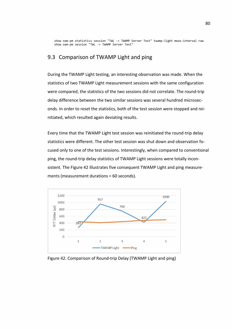
80
show oam-pm statistics session "TWL -> TWAMP Server Test" twamp-light meas-interval raw show oam-pm session "TWL -> TWAMP Server Test"
9.3 Comparison of TWAMP Light and ping
During the TWAMP Light testing, an interesting observation was made. When the
statistics of two TWAMP Light measurement sessions with the same configuration
were compared, the statistics of the two sessions did not correlate. The round-trip
delay difference between the two similar sessions was several hundred microsec-
onds. In order to reset the statistics, both of the test session were stopped and rei-
nitiated, which resulted again deviating results.
Every time that the TWAMP Light test session was reinitiated the round-trip delay
statistics were different. The other test session was shut down and observation fo-
cused only to one of the test sessions. Interestingly, when compared to conventional
ping, the round-trip delay statistics of TWAMP Light sessions were totally incon-
sistent. The Figure 42 illustrates five consequent TWAMP Light and ping measure-
ments (measurement durations = 60 seconds).
Figure 42. Comparison of Round-trip Delay (TWAMP Light and ping)

81
It seemed like re-initiation of TWAMP Light session generated a random value for the
round-trip delay statistic. Even if the test session was observed a longer period of
time, the results were the same. If the average round-trip delay started high, it also
remained high. It would have been reasonable, if the long-term statistics had been
adjusted near (or even below) to the more consistent delay value measured with
ping. Theoretically, this would have been correct, especially when TWAMP Light test
packets were marked as highest priority forwarding class. To experiment more,
TWAMP Light session controllers were configured to me-s01, me-s02 and me-s03 de-
vices. TWAMP Light responder functionality was configured to all named devices in
Figure 43.
Figure 43. TWAMP Light Test Sessions
Two separate measurement sessions were conducted. Each of the two sessions was
observed when approximately 1 000, 2 000 and 3 000 test packets were received by

82
the session controllers. The observations in the Table 6 are presented in microsec-
onds, where column A represents the observation at 1000 test packet milestone.
Similarly, column B equals to 2 000 and column C to 3 000 received test packets.
Table 6. Round-trip Delay (TWAMP Light)
Session 1 Session 2
Controller Reflector A B C Min Max A B C Min Max
me-s01
me-s02 650 652 653 645 665 134 136 137 128 137
me-s03 49 49 49 44 56 49 49 39 45 59
met-s15 70 70 70 67 78 70 70 70 67 78
me-s19 70 70 70 67 80 70 70 70 67 78
me-s20 61 61 61 55 71 61 61 61 55 69
me-s02 me-s01 755 755 755 751 764 270 270 270 264 270
me-s03 734 734 734 729 743 298 298 298 292 298
me-s03 me-s01 49 49 49 44 55 49 49 49 44 55
me-s02 790 794 798 783 818 245 250 254 238 254
Based on the results, it seemed that me-s02 was actually only device, which had is-
sues reporting consistent statistics. When compared to ping, me-s02 performed simi-
larly than me-s03 giving consistent round-trip delay statistics. Table 7 presents a ref-
erence statistics measured from me-s01 using ping.
Table 7. Round-trip Delay (Ping) Source Destination Ping1 Ping2 Ping3 Ping4 Ping5
me-s01
me-s02 338 369 334 354 344
me-s03 334 338 334 332 349
met-s15 476 466 494 619 692
me-s19 494 506 467 436 523
me-s20 372 383 388 342 376
Assuming round-trip delays measured with TWAMP Light are reliable, the time re-
quired to process ICMP packets is few hundred microseconds. As the fiber connec-
tion were short in the laboratory environment (up to 15 meters), the results in Table
6 correlate well with theoretical minimum round-trip delay values, which in really
short connections should be around 20 µs. me-s02 and me-s03 seemed to perform

83
better compared to other nodes, which were lower-end equipment. The reason why
me-s02 did not perform well in TWAMP Light measurement sessions remained un-
known.
10 Latency Tests
10.1 Preparation
Ping was selected as a measurement method, because it was most likely capable of
delivering accurate enough statistics on millisecond scale. The biggest drawback of
TWAMP Light was its scalability compared to ping, which was more flexible of gather-
ing and logging arrays of measurement data. TWAMP Light measurements would
have required CPU stress testing and additionally testing of packet generation capa-
bilities of the devices, which would have been used as TWAMP Light clients. The
measurement statistics presented in this and the following chapters represent the
real data gathered from measurement sessions. Some parts of the measurement
data and configuration examples such as device names, locations details and IP ad-
dresses are masked or hidden as they are not public part of the thesis.
The measurements were conducted individually for each regional network by using a
Unix server dedicated for network management functions. This approach added
some uncertainty since Telia’s management network had dozens of connections to
production network. Therefore, before any measurements could be conducted, it
was necessary to determine the names of the ME nodes and the routes to regional
networks. First, the names of all ME nodes in each region were polled using SNMP.
The following snmpwalk command queries all ME nodes that belong to the same re-
gion as me-node1. The command also parses the query and writes the nodes’ DNS
names into areaA file:

84
snmpwalk -v 2c -c example me-node1 .1.3.6.1.4.1.x.y.z | grep ' "me-' | awk '{print $4}' | sed 's/"//g' > areaA
The next step was using traceroute to determine the forward routes for the test
packets as well as the ME nodes that connected regional networks to the manage-
ment network. A bash script was made for running multiple traceroutes to the nodes
in the same region, however, for some reason traceroute could not be initiated with
the script file:
traceroute: icmp socket: Permission denied
Consequently, it was necessary to issue traceroute commands by sequencing them
directly from the CLI (1) and grep node names from areaA-trc file to create areaA-hps
file (2), which contained the number of hops and DNS names of the nodes (3):
(1) traceroute me-node1 >> areaA-trc; traceroute me-node2 >> areaA-trc; ... (2) more areaA-trc | grep me- > areaA-hps (3) ...
7 me-node1 (<IP address>) 1.088 ms 1.120 ms 1.103 ms 6 me-node2 (<IP address>) 1.229 ms 1.107 ms 1.248 ms ...
Examination of the two generated files revealed the ME node connecting the man-
agement network to the regional network (least amount of hops) as well as the
routes to the ME nodes within the region. The ME nodes interconnecting the man-
agement and regional networks were directly connected to a ME core node in each
region (as shown in Figure 44).

85
Figure 44. Measurement Topology I
The red dotted line in the above figure represents the forward and reverse paths of a
ping packet. For comparison, the blue dotted line represents the round-trip path of
an IP packet when ping is initiated from a ME access node (MEa). In this example, the
blue path is the best forwarding path for traffic from the ME access node and repre-
sents the shortest possible ‘regional latency’. As shown in the figure, in some cases
the measurement setup added additional delay to the statistics gained from the
measurements. Although sending ping packets from the management server was not
optimal, it was the only alternative with the available timeframe due to major issues
with user accounts and permissions required to get access to production network de-
vices.
10.2 fping
The measurements were conducted using fping program, which was an alternative
for utilizing bash script language with Unix’s built-in ping program. Both of the pro-
grams’ delay statistics were in the same magnitude; however, eventually fping was

86
selected due to its suitability for pinging multiple hosts and collecting large amounts
data. The Figure 45 presents the measurement topology, which highlights the re-
gional latency in service-perspective with blue dotted lines. The red dotted line rep-
resents the delay caused by management network, which was subtracted from the
overall delay of individual measurements.
Figure 45. Measurement Topology II
The amount of test packets sent to each ME node was 120 and multiple measure-
ments were conducted using 84-byte and 1500-byte packet sizes. The command (1)
shown below sends 120 ICMP echo requests to each ME node present in areaA file,
labels statistics of individual test packets with a Unix time stamp and writes them to
areaA-vrb file. The output (2) displays the contents of the file:

87
(1) fping -C 120 -D < areaA >> & areaA-vrb (2) [1523699889.755149] me-node75 : [49], 84 bytes, 6.60 ms (6.79 avg, 0% loss) [1523699889.780036] me-node76 : [49], 84 bytes, 6.45 ms (6.51 avg, 0% loss) [1523699889.804812] me-node77 : [49], 84 bytes, 5.99 ms (6.05 avg, 0% loss) me-node1 : 5.80 5.74 5.71 5.71 5.70 5.65 5.73 5.69 5.83 5.65 5.56 5.80 5 .69 6.10 5.74 5.71 5.92 5.64 5.74 5.65 5.75 5.92 5.81 5.80 5.89 5.78 5.81 5.84 5 .70 5.71 5.76 5.72 5.80 5.80 5.78 5.87 5.92 5.78 5.90 5.88 5.44 5.71 5.58 5.78 5 .73 5.70 5.69 5.83 5.77 5.79
Due to the volume of measurement statistics (136,680 individual records per meas-
urement = 120 test packets sent to all ME nodes), the data was exported to Excel
where it was easier to analyze. In order to do this, the data required parsing. The fol-
lowing command finds the rows starting with me-, adds a string AreaA with a space
as a delimiter and removes all tabular keystrokes as well as colons:
more areaA-vrb | grep "^me-" | awk '{print "areaA " $0}' | sed 's/ //g' | sed 's/://g' > areaA-sts
After the data was parsed, it was analyzed in Excel where it was enriched by adding
information such as device models, technical sites and geographical locations from
Telia’s inventories. In addition, the number of hops was included as it helped as-
sessing the reliability of the measured data. The statistics presented in Figure 46 rep-
resent real round-trip delay statistics from a regional network. The columns in the
figure include: measured delay (minimum, median and average) of the 120 test pack-
ets, ratio of measured average and median delay, variance and standard deviation of
measured delay as well as delay statistics of the ME core node, which were sub-
tracted from the measured values (the estimated delay is displayed in Min, Median,
Average and Max columns). The delay statistics of individual test packets are shown
on the right side of the figure beside the Hops column. In the figure, one row repre-
sents statistics of a ME node.

88
Figure 46. Round-trip Delay Statistics
11 Results
11.1 Analysis
Even if the actual measurement was straightforward, analysis of the data gathered in
multiple measurement sessions was much more complex. The analysis required ex-
amining the complete traceroute data together with technical drawings and infor-
mation gathered using 5620 SAM. Although the drawings included IS-IS metrics and
approximate geographical locations of the ME nodes, one of the most time consum-
ing tasks was to investigate the actual routes to the remote measurement points. Be-
cause traceroute reported link addresses, there was no easy way to determine, to
which of the nodes the link addresses belonged.
The first observation of the measurement data was that the statistics were coherent.
In overall, the average delay correlated well with the median delay, which made the
data mathematically symmetric. There was also no significant packet loss, as the

89
highest recorded test packet loss was 0.000055% (which equals to 15 lost ICMP pack-
ets when 273,360 packets were sent). Considering the average and median delay,
99.6% of the measured ME nodes were under 8 ms limit. The percentage for 5 ms
limit was 95.3%. (Note: These are the results of three separate measurements)
The comparison of maximum delay did not prove useful, as sometimes there were
individual test packets with high delay while the other test packets were near to min-
imum measured round-trip time. However, there were nodes, which reported high
maximum values in patterns (e.g. every other test packet reported 10 ms greater de-
lay than the previous test packet) indicating possible issues. In addition, a compari-
son of average delay was less useful as significantly high maximum values raised the
average delay considerably. For most of the nodes, there was a rather small differ-
ence of 300 µs between median and minimum delay, which indicated that routers re-
sponded to ICMP echo requests in uniform, considering that the intention was only
to produce millisecond-level data with the ping measurements.
ME nodes physically connected to management network (from now on referred as
MEm nodes) performed consistently, i.e. usually the measured round-trip delay was
almost the same. Although the overall results of the MEm nodes were consistent,
there were individual test packets with greater delay. Based on the results, MEms
which were 7750 SR-12, 7450 ESS-12 or 7450 ESS-7 series equipment, were not al-
ways the fastest nodes to respond to ICMP echo requests. It was evident that ESS se-
ries equipment responded considerably slower to ping than SR series equipment,
which were further in the topology on a same or even a different site. This can be
seen in Figure 47 where the only ‘better performing’ ESS series node is the first node
present in the figure.

90
Figure 47. Comparison of Round-trip Delay Statistics
The figure above illustrates the three fastest (minimum delay of 120 test packets) ME
nodes from eight individual regional networks. The dots highlight the MEms, which
are the closest nodes to the ping source (the management server). Note that the fig-
ure also contains negative values as the measured delay from management server to
SR-12s was usually smaller, and because the greater delay (delay from management
server to ESS-12s) it was subtracted from the total measured round-trip delay.
The raw measurement data (Dr) was only useful when comparing ME nodes within a
single region. For this reason, the estimated round-trip delay (De) was calculated by
subtracting the delay (Dm) resulting from management network (refer to Figure 48).
This means that the amount of subtracted round-trip delay Dm is always the same for
every ME node in a region per measurement. Since this subtraction was necessary,
there is an error margin, as there is a difference between ME nodes’ capability to
handle ICMP echo requests.

91
Figure 48. Delay Components I
For example, Dm is 2 400 µs and the amount of time test packet spends in the control
plane of the device (DICMP) is 300 µs. If another node from the same region is meas-
ured, and the total round-trip time is Dr 4 600 µs, then according to calculation logic
De is 2 200 µs. If DICMP in this case had been instead 450 µs (assuming 450 µs DICMP
stays constant), the measured round-trip delay would have been 2 350 µs, when
pinging the node directly from a ME core node. If all device models’ ICMP processing
capabilities were similar, the delay resulting from ICMP packet processing would be
theoretically non-existent as shown in Figure 49.

92
Figure 49. Delay Components II
The most distinguishable factor contributing to the overall delay was the distance. If
the distance between nodes was long, also the number of hops correlated well with
the data. Another factor was the packet size. When comparing Dr of 84 byte and
1500 byte packets, the 1500-byte packet size increased the minimum and average
delay of all measured equipment by 0.9 ms compared to smaller test packets. How-
ever, when Dm was subtracted there was no significant difference, indicating that the
increased test packet size seemed only to measure the ICMP processing capability of
the ME nodes.
There were only minor differences when comparing statistics of two separate meas-
urements sessions with the same packet size (84-byte packets). Table 8 presents the
difference, where the column < 100 µs indicate how many of the ME nodes re-
sponded to ping within ± 100 µs time frame. Correspondingly, < 200 µs indicates the
amount of ME nodes, which managed to respond within ± 200 µs. Based on the re-
sults, the response rates were quite consistent as there are only few nodes present
in the > 200 µs column (excluding less indicative average delay).

93
Table 8. ME Node Response Rates within Time Intervals
< 100 μs < 200 μs > 200 μs
Minimum 1051 (92.3 %) 1137 (99.8 %) 2 (0.2 %)
Median 1103 (96.8 %) 1134 (99.6 %) 5 (0.4 %)
Average 875 (76.8 %) 1029 (90.3 %) 110 (9.7 %)
To determine the reliability of the results, it was also necessary to calculate the theo-
retical minimum delay values, which were compared to actual results. Due to num-
ber of equipment measured, only a number of calculations were made. Calculations
assumed 10 µs switching delay, since no response was received from Nokia about
switching delay of the equipment in the scope. All calculations also assumed 0 ms
scheduling delay as regional networks did not contain any saturated links between
the ME nodes. Technically, there was a possibility that some test packets were sched-
uled as the overall port utilization rate is calculated from a certain interval. Moreo-
ver, the utilization rate of the links in management network was not known during
the measurements.
The propagation delay was calculated based on the actual cable lengths recorded in
Telia’s inventories and serialization delay based on the actual link speeds. Figures 50
and 51 present the results of calculations and the minimum De for two packet sizes.
The theoretical values for both packet sizes are almost equal, as packet size in 10
Gbps links is an insignificant factor contributing to overall delay. There is also a minor
error margin in switching delay because smaller packet sizes require less processing
in the data plane. The milliseconds represent the round-trip time while kilometers
represent the length of the cable route, and therefore, they do not represent the
‘round-trip distance’ of the test packets.

94
Figure 50. Comparison of Round-trip Delay Statistics (Theoretical vs. Actual) I
Figure 51. Comparison of Round-trip Delay Statistics (Theoretical vs. Actual) II
Based on the above figures, there is a difference between the measured and theoret-
ical round-trip delay – which was expected. The possible reason why the delay differ-
ence is the greatest in the end of the cable route is that these two examples had

95
lower-tier ME nodes in the remote end. Since the ME core nodes were the fastest
nodes to respond to ICMP echo requests, their DICMP was the lowest. The delay differ-
ence mostly likely grows as lower-tier ME nodes respond slower to ping (DICMP is
greater).
11.2 Conclusions
Since high percentage of ME nodes (99.6 %) were under 8 ms limit, the overall delay
performance of the network is likely sufficient for early 5G applications. The statistics
are not absolute, which means the measurement statistics are very likely greater
than actual values due to variation in ICMP packet processing. In addition, TWAMP
Light measurements support this. The comparison of TWAMP and ping revealed that
the measured delay difference in laboratory environment was significant, when the
links between the nodes were short. The probable reasons are most likely that there
was insignificant amount of propagation delay and the most decisive delay compo-
nent was high DICMP of Nokia’s network equipment.
Presumably, the difference in TWAMP and ping delay statistics will be smaller, when
the distance between measurement points are greater. As a result, the decisive fac-
tor affecting to overall delay would be caused by signal propagation, naturally de-
pending on the amount actual DICMP. As shown in the equation, the distance is the
primary delay factor in longer links (five 40 kilometer link sections, 10 μs switching
delay and 0 μs scheduling delay are assumed):
𝐷𝑡𝑜𝑡 = 2 {𝑁(𝐷𝑠𝑒𝑟 + 𝐷𝑝𝑟𝑜 + 𝐷𝑠𝑤𝑖 + 𝐷𝑠𝑐ℎ)} + 𝐷𝐼𝐶𝑀𝑃
𝐷𝑡𝑜𝑡 = 2 {5(1 𝜇𝑠 + 200 𝜇𝑠 + 10 𝜇𝑠 + 0 𝜇𝑠)} + 𝐷𝐼𝐶𝑀𝑃
𝐷𝑡𝑜𝑡 = 2 110 𝜇𝑠 + ?

96
where 𝐷𝑠𝑒𝑟 = 𝑏𝑖𝑡𝑠
𝑠𝑙𝑖𝑛𝑘 =
1522 𝑏𝑦𝑡𝑒𝑠
10 𝐺𝑏𝑝𝑠 and 𝐷𝑝𝑟𝑜 = 5 𝑚𝑠 (𝑝𝑒𝑟 1000 𝑘𝑚)
Although ping does not represent TWAMP-like accuracy, it clearly correlates with the
distance, which is the most decisive delay factor in large-scale networks. The most
problematic parts of the network are clearly the nodes, which are far from the core
sites. However, even if the nodes are not very far from the core sites, the length of
redundant routes is also a problem. The highest measured median round-trip delay
was 9.67 ms due to the length of an alternative WDM route, which was preferred be-
cause of its greater capacity compared to considerable shorter fiber route.
An overview of the measurement statistics can be seen in Appendix 8 where meas-
urement data is sorted by median delay per region. The appendix does not contain
any actual numeric values as they are not the public part of this thesis. The appendix
rather visualizes the coherence of data for four separate regional networks using a
green-yellow-red formatting.
11.3 Improvements and Recommendations
Because the difference of observed round-trip delay of ping and TWAMP Light meas-
urements was several hundred milliseconds, it is recommendable to conduct TWAMP
Light measurements in regional networks in order to determine the correctness of
the statistics measured in this research. In addition, the access network layer, includ-
ing some regional nodes dedicated to backhaul the mobile traffic, was excluded from
the scope of the thesis. Therefore, this research does not indicate the end-to-end la-
tency between base stations and the mobile core, leaving room for future end-to-
end measurements from service-perspective. Most importantly, the delay for alter-
native routes was not measured, which is important, as network faults and planned
maintenances force the traffic to routes that are not preferred in normal conditions.

97
Arranging fault scenarios voluntarily to production network is not an option, meaning
there is likely a need to measure the delay of individual links in order to determine
the delay of the longest routes.
Concerning TWAMP, there are use cases, which require further investigation. For ex-
ample, an additional research question was raised during the TWAMP Light testing
concerning TWAMP Light’s suitability for monitoring LAGs (Link Aggregation Group).
Another topic that remained uninvestigated was how to collect TWAMP Light statis-
tics effectively from the ME nodes if external probes are not used to send test pack-
ets. This, as a result, requires some testing as routers and switches are not primarily
built for generating traffic, and because CPU stress of the TWAMP Light measure-
ment sessions is not known. Implementing TWAMP Light is beneficial due to its abil-
ity to measure one-way statistics indicating possible latency issues per direction and
because it would likely provide reliable delay variation statistics, of which ping is not
capable.
When the final results of were introduced to the stakeholders in Telia’s organization,
especially the presentation of the data made an impression. There is already a plan
to implement scheduled script, which will utilize a ping program and transfer statis-
tics automatically to Splunk application. This easy-to-implement method should pro-
vide an automatic overview of the nodes that for some reason have problems reply-
ing ICMP echo request messages. Although slow ICMP echo response rate might not
indicate clearly of any specific issue, displaying ping statistics (also possibly trac-
eroute statistics) in real-time should provide a proactive tool for network monitoring.
Splunk integration will also save time, since gathering measurement statistics to an
Excel file took approximately five minutes of manual effort per measurement.

98
12 Discussion
Ping is not a reliable method of measuring latency. Regardless, ping is a simple
method of measuring latency and provides a very cost-effective way to get a baseline
of the network quickly without making any investments in software or probes.
Hence, ping clearly can correlate well enough in measurements, which does not re-
quire near absolute delay statistics. In addition, combining simple data such as num-
ber of traceroute hops did reveal unexpectedly routing issues in both production and
management network. For example, one finding was that there was a 6-hop differ-
ence between two directly connected nodes, which meant an additional round-trip
delay of 1.14 ms, resulting only from signal propagation as alternative 114 kilometer
longer route was used. The root cause for the finding was a missing LDP configura-
tion that prevented all traffic forwarding via the preferred shorter link.
The subject of the thesis was extremely interesting and provided a great lookout spot
to study Telia’s network architecture. Both the thesis process, as well as the technol-
ogies studied in this research, provided an educative opportunity (which was, by the
way, eagerly accepted) to improve the knowledge of an operator-tier IP network.
However, the thesis subject was quite demanding, as it contained two individual
practical phases and required a great deal of familiarization with Telia’s network ar-
chitecture. Although the constraints of the thesis were clear, it was hard to estimate
the amount of effort required to complete all of the tasks. It was particularly hard to
assess the reliability of an unreliable measurement protocol.
Although the latency tests were eventually conducted using a simple method, work-
ing in a foreign and complex laboratory environment with new SR operating system
was not exactly easy. As my tasks in normal daily work at Telia did not relate at all to
networking, the main delay elements in the thesis process were schedule-related

99
due to workload of a major project in Telia, and getting necessary access rights and
permissions to be able to access and configure the network elements. Working with
two completely different issues made it very hard to keep the focus on both the the-
sis process and the daily work at the same time. Nevertheless, the primary objective
was achieved by providing the essential information for the organization.
The results of this research identify the areas of regional networks requiring optimi-
zation and guide the network planning for 5G. By comparing earlier historic measure-
ment statistics to the most current statistics, regular measurements should indicate
configuration issues relating to routing, and how network topology changes affect
the delay. Regular measurements also likely add value to planning of customer solu-
tions requiring low latency as well as may help identifying faults of latency-critical
customers. (Kivirinta 2018.)
The statistics are useful especially for the designers and technicians familiar with net-
work topologies. Although the full value of the results of the thesis cannot be esti-
mated for certain, the measurements for the baseline have already been proven val-
uable by pointing out a configuration issue in the production network. There was
only one finding, since only one of the regional networks’ measurement statistics
was analyzed more thoroughly by comparing the statistics to the physical topology.
Only the most familiar topology was selected, as full analysis of all of the regions’ sta-
tistics would have required another thesis. The research results relating to TWAMP
testing may prove useful at some point, however, that is to be seen when TWAMP
testing becomes relevant in the near future.
Telia, likely along with the other service providers, plans to introduce the future 5G
network gradually, where 5G network is integrated with the existing 4G network ar-
chitecture. This enables securing the infrastructure for early 5G applications, such as

100
eMBB, which is likely the first 5G service category to be introduced. This also means
that the rest of the more advanced 5G usage cases relating to augmented reality and
industrial automation will be introduced as a service later. Most likely, the most
stringent latency-critical uRRLC applications are the last to be introduced. It will be
interesting to see whether the most remote rural areas far from larger cities will ever
support uRRLC usage cases as – well… One millisecond is a very short period of time.
To meet the requirement in every corner within a geographically large and sparsely
populated country requires an overhaul of the entire mobile core architecture. This,
instead, would greatly increase the overall cost of constructing 5G, making it an un-
reasonable investment.
It might be easy to think that once the upcoming 5G standard is finished, the vendors
can start creating high-end equipment dedicated to delay mitigation, and the equip-
ment is then installed to service provider networks. From a service provider’s per-
spective, investing into the high-end technology will require a valid business case to
justify the reason to invest. This means also that the customers need to be willing to
acquire high-end services that are not likely cheap. The commercialization of 5G net-
works is the next major milestone in the evolution of mobile networks, which is why
it will be worth waiting to see what exactly that means in practice – and what exactly
it actually changes.

101
References
10 Year Review of TeliaSonera. 2013. CEO’s letter to the shareholders of Teliasonera. Accessed on 3.4.2018. Retrieved from https://www.teliacompany.com/globalassets/telia-company/documents/about-telia-company/TeliaSonera_Letter-to-Shareholders_Telia-10-Years_2013.pdf
3GPP TS 23.501 v15.0.0. 2017. System Architecture for the 5G System. Technical specification by 3GPP. Accessed on 30.4. Retrieved from https://portal.3gpp.org/desktopmodules/Specifications/SpecificationDetails.aspx?specificationId=3144
7450 ESS, 7750 SR, 7950 XRS, and VSR OAM and Diagnostics Guide R15.1.R1. 2017. Nokia’s OAM and Diagnostics Guide.
Alcatel-Lucent 7740 SR OS Routing Protocols Guide. 2015. Routing Protocol Guide for 12.0 R4 OS version.
Annual and Sustainability Report. 2017. Telia’s 2017 sustainability report. Accessed on 3.4.2018. Retrieved from https://annualreports.teliacompany.com/globalassets/2017/pdf/engelska-pdf/teliacompany_ar2017_eng.pdf
Bäckström, I. 2009. Performance Measurement of IP Networks using the Two-Way Active Measurement Protocol. Master’s Thesis. Accessed on 3.5.2018. Retrieved from https://www.nada.kth.se/utbildning/grukth/exjobb/rapportlistor/2009/rapporter09/backstrom_ingmar_09038.pdf
Carrell, J., Kim, D. & Solomon, M. 2015. 2nd edition. Fundamentals of Communications and Networking. E-book.
CCNA 1 and 2 Companion Guide. 2005. 3rd edition. Indianapolis: Cisco Press.
Evans, J. & Filsfils, C. 2007. Deploying IP and MPLS QoS for Multiservice Networks. San Francisco: Morgan Kaufmann Publishers.
https://portal.3gpp.org/desktopmodules/Specifications/SpecificationDetails.aspx?specificationId=3144

102
Geary, J., Martin-Löf, J., Sundelius, C. & Thorngren, B. 2010. The History of Telia. Compilation of history of TeliaSonera. Accessed on 30.4.2018. Retrieved from http://thorngren.nu/wp-content/uploads/2014/03/The-History-of-Telia.pdf
Ghafary, M., Shaheen, G. & Warnock, G. 2015. Alcatel-Lucent Service Routing Architect (SRA) Self-Study Guide. E-book.
Goralski, W. 2009. The Illustrated network: How TCP/IP Works in Modern World. E-book.
Hundley, K. 2009. Alcatel-Lucent Scalable IP Networks Self-Study Guide. Indianapolis: Wiley Publishing.
Huston, G. 2003. Measuring IP Network Performance – The Internet Protocol Journal – Volume 6, Number 1. Kuvaus. Accessed on 12.3.2018. Retrieved from https://www.cisco.com/c/en/us/about/press/internet-protocol-journal/back-issues/table-contents-23/measuring-ip.html
IP SLAs Configuration Guide, Cisco IOS XE Release 3S. 2018. Cisco’s configuration guide for IP SLAs TWAMP Responder. Accessed on 11.4.2018. Retrieved from https://www.cisco.com/c/en/us/td/docs/ios-xml/ios/ipsla/configuration/xe-3s/sla-xe-3s-book/sla_twamp.html
KB27335. N.d. Latency or delay in processing ICMP response when pinging the EX series switch. Accessed on 15.5.2018. Retrieved from https://kb.juniper.net/InfoCenter/index?page=content&id=KB27335&cat=EX_SERIES&actp=LIST
Kim, Y., Kishiyama, Y., Liu, G., Ma, J., Parkvall, S., Ye Li, G & Zhang, C.,. 2018. Key Technology for 5G New Radio. Article. Accessed on 8.4.2018. Retrieved from http://ieeexplore.ieee.org/document/8316580/
Kivirinta, R. 2018. Written statement from Telia’s planning department (core and aggregation networks).
M.2083-0. IMT Vision – Framework and overall objectives of the future development of IMT for 2020 and beyond. 2015. Recommendation for IMT-2020 by ITU-R. Accessed on 3.4.2018. Retrieved from https://www.itu.int/dms_pubrec/itu-r/rec/m/R-REC-M.2083-0-201509-I%21%21PDF-E.pdf

103
Marschke, D., Reynolds, H & Southwick, P. 2008 JUNOS Enterprise Routing: Practical Guide to JUNOS Software and Enterprise Certification. E-book.
Miller, K. Calculating Optical Fiber Latency. 2012. Article on M2 Optics’ web page. Accessed on 9.4.2018. Retrieved from http://www.m2optics.com/blog/bid/70587/Calculating-Optical-Fiber-Latency
Monge, A. & Szarkowicz, K. 2015. MPLS in the SDN Era. E-book. Accessed on 3.5.2018. Retrieved from https://www.safaribooksonline.com/library/view/mpls-in-the/9781491905449/ch01.html
Nucci, A. & Papagiannaki K. 2009. Design, Measurement and Management of Large-Scale IP Networks: Bridging the Gap Between Theory and Practice. E-book.
Odom, W. 2011. CCENT/CCNA ICND1 640-822 Official Cert Guide. 3rd edition. Accessed on 1.4.2018. Retrieved from http://www.ciscopress.com/articles/article.asp?p=1757634&seqNum=2
Oki, E., Rojas-Cessa, R., Tatimapula, M. & Vogt, C. 2012. Advanced Internet Protocols, Services, and Applications. E-book.
Pepelnjak, I. 2013. OpenFlow and SDN: Hype, Useful Tools or Panacea? Presentation. Accessed on 29.4.2018. Retrieved from https://www.menog.org/presentations/menog-12/115-OpenFlow_and_SDN_(MENOG).pdf
Raza, K. & Turner, M. 1999. CCIE Professional Development Large-Scale IP Network Solutions. Indianapolis: Cisco Press.
RFC 1122. 1989. Requirements for Internet Hosts -- Communication Layers. Internet Standard (IETF). Accessed on 4.4.2018. Retrieved from https://tools.ietf.org/html/rfc1122
RFC 3031. 2001. Multiprotocol Label Switching Architecture. Proposed standard (IETF). Accessed on 26.8.2017. Retrieved from https://tools.ietf.org/html/rfc3031
RFC 3032. 2001. MPLS Label Stack Encoding. Proposed standard (IETF). Accessed on 26.8.2018. Retrieved from https://tools.ietf.org/html/rfc3032

104
RFC 4656. 2006. A One-way Active Measurement Protocol (OWAMP). Proposed standard (IETF). Accessed on 1.4.2018. Retrieved from https://tools.ietf.org/html/rfc4656
RFC 5357. 2008. A Two-Way Active Measurement Protocol (TWAMP). Proposed standard (IETF). Accessed on 1.4.2018. Retrieved from https://tools.ietf.org/html/rfc5357
RFC 5618. 2009. Mixed Security Mode for the Two-Way Active Measurement Protocol (TWAMP). Proposed standard (IETF). Accessed on 3.9.2017. Retrieved from https://tools.ietf.org/html/rfc5618
RFC 7799. 2016. Active and Passive Metrics and Methods (with Hybrid Types In-Between). Informational RFC (IETF). Accessed on 1.4.2018. Retrieved from https://tools.ietf.org/html/rfc7799
RFC 791. 1981. Internet Protocol. Internet standard (IETF). Accessed on 19.4.2018. Retrieved from https://tools.ietf.org/html/rfc791
RFC 792. 1981. Internet Control Message Protocol. Internet Standard (IETF). Accessed on 16.4.2018. Retrieved from https://tools.ietf.org/html/rfc792
Service Level Monitoring with Cisco IOS Service Assurance Agent. N.d. White Paper. Accessed on 1.4.2018. Retrieved from http://www.cisco.com/en/US/tech/tk648/tk362/technologies_white_paper09186a00800e9012.shtml
Shuttleworth, M. N.d. Quantitative Research Design. Article on Explorable’s web page. Accessed on 15.5.2018. Retrieved from https://explorable.com/quantitative-research-design
Telia Carrier – Network Map. N.d. Accessed on 3.4.2018. Retrieved from http://www.teliacarriermap.com/
Telia Carrier – Services. N.d. Accessed on 19.4.2018. Retrieved from https://www.teliacarrier.com/our-services.html

105
TWAMP Explained. 2014. TWAMP Explained. Presentation of TWAMP by RAD Data Communications on SlideShare’s web page. Accessed on 1.2.2018. Retrieved from https://www.slideshare.net/nirc1963/what-istwamp
Understanding Two-Way Active Measurement Protocol on Routers. 2018. Description of Juniper TWAMP architecture. Accessed on 11.4.2018. Retrieved from https://www.juniper.net/documentation/en_US/junos/topics/concept/twamp-overview.html
Unicast Routing Protocols Guide Release 15.1.R1. 2017. Nokia’s guide for 7450 ESS, 7750 SR, 7950 XRS and VRS series equipment.
VNI Forecast Highlights Tool. N.d. Cisco’s Visual Networking Index Tool. Accessed on 2.4.2018. Retrieved from https://www.cisco.com/c/m/en_us/solutions/service-provider/vni-forecast-highlights.html
Y.1540. 2016. Internet protocol data communication service – IP packet transfer and availability performance parameters. Recommendation by ITU-T.
Zhao, H. 2017. 5G update: New ITU standards for network softwarization and fixed-mobile convergence. Article on ITUNews’ web page. Accessed on 3.4.2018. Retrieved from http://news.itu.int/5g-update-new-itu-standards-network-softwarization-fixed-mobile-convergence/
Zhao, H. 2018. How ITU helps to create a new mobile era via 5G. Article on ITUNews’ web page. Accessed on 3.4.2018. Retrieved from http://news.itu.int/itu-helps-create-new-mobile-era-via-5g/

106
Appendices
National Network Layers

107
5QI QoS Characteristics mapping

108
Request-TW-Session Message (RFC 4656 2006, 14)

109
TWAMP/TWAMP Light Commands in SR OS 14.0.R4 TWAMP configure — test-oam — twamp — server — [no] prefix {address/prefix-length} [create] — description text — no description — max-conn-prefix count — no max-conn-prefix — max-sess-prefix count — no max-sess-prefix — [no] shutdown — inactivity-timeout seconds — no inactivity-timeout — max-conn-server count — no max-conn-server — max-sess-server count — no max-sess-server — shutdown TWAMP Light configure — router — twamp-light — reflector [udp-port udp-port-number] [create] — no reflector — description description — no description — prefix {ip-prefix/prefix-length} [create] — no prefix — description description — no description — [no] shutdown configure — service — vprn —[no] twamp-light — reflector [udp-port udp-port-number] [create] — no reflector — description description — no description — prefix — no prefix — description description — no description — [no] shutdown configure — test-oam — twamp — twamp-light — inactivity-timeout seconds — no inactivity-timeout configure — oam-pm — session — ip — destination ip-address

110
— no destination — dest-udp-port udp-port-number — no dest-udp-port — fc fc-name — no fc — forwarding {next-hop ip-address | interface interface-name | bypassrout ing} — no forwarding — profile {in | out} — no profile — router {base | routing-instance | service-name service-name} — no router — source ip-address — no source — source-udp-port udp-port-number — no source-udp-port — ttl time-to-live — no ttl — twamp-light [test-id test-id][create] — no twamp-light — interval milliseconds — no interval — loss — flr-threshold percentage — [no] flr-threshold — timing frames-per-delta-t frames consec-delta-t deltas chli-threshold threshold — [no] timing — loss-events — avg-flr-event {forward | backward} threshold raisethreshold- percent [clear clear-threshold-percent] — [no] avg-flr-event {forward | backward} — chli-event {forward|backward|aggregate} threshold raise-threshold [clear clear-threshold] — [no] chli-event {forward|backward|aggregate} — hli-event {forward|backward|aggregate} threshold raise-threshold [clear clear-threshold] — [no] hli-event {forward|backward|aggregate} — unavailability-event {forward|backward|aggregate} threshold raise-threshold [clear clear-threshold] — [no] unavailability-event{forward|backward|aggregate} — undet-availability-event {forward|backward|aggregate} threshold raisethreshold [clear clear-threshold] — [no] undet-availability-event{forward|backward|aggregate} — undet-unavailability-event {forward|backward|aggregate} threshold raisethreshold [clear clear-threshold] — [no] undet-unavailability-event {forward|backward|aggregate} — pad-size octets — no pad-size — pad-size — record-stats {delay | loss | delay-and-loss} — [no] record-stats — [no] shutdown — test-duration seconds — no test-duration

111
PM Session Configuration

112

113
TWAMP Light Session Configuration B:me-s02>config>oam-pm>session# info detail ---------------------------------------------- bin-group 1 description "Test for TWL packet reflection from TWAMP server" meas-interval 15-mins create no accounting-policy boundary-type clock-aligned clock-offset 0 event-mon shutdown no delay-events no loss-events exit intervals-stored 32 exit ip dest-udp-port 49152 destination <IP address> fc "be" no forwarding profile out router "Base" source <IP address> source-udp-port 64374 ttl 255 twamp-light test-id 5 create shutdown interval 1000 loss flr-threshold 50 timing frames-per-delta-t 1 consec-delta-t 10 chli-threshold 5 exit loss-events no avg-flr-event forward no avg-flr-event backward no chli-event forward no hli-event forward no unavailability-event forward no undet-availability-event forward no undet-unavailability-event forward no chli-event backward no hli-event backward no unavailability-event backward no undet-availability-event backward no undet-unavailability-event backward no chli-event aggregate no hli-event aggregate no unavailability-event aggregate no undet-availability-event aggregate no undet-unavailability-event aggregate exit pad-size 27 record-stats delay-and-loss no test-duration exit exit ----------------------------------------------

114
TWAMP Light Session: me-s02 B:me-s02>config>oam-pm>session# show oam-pm statistics session "TWL -> TWAMP Server Test" twamp-light meas-interval raw ------------------------------------------------------------------------------ Start (UTC) : 2018/04/17 11:07:58 Status : in-progress Elapsed (seconds) : 371 Suspect : yes Frames Sent : 371 Frames Received : 371 ------------------------------------------------------------------------------ =============================================================================== TWAMP-LIGHT DELAY STATISTICS ---------------------------------------------------------------------- Bin Type Direction Minimum (us) Maximum (us) Average (us) ---------------------------------------------------------------------- FD Forward 500576702 500579818 500578260 FD Backward 0 0 0 FD Round Trip 563 574 566 FDR Forward 0 3116 1558 FDR Backward 0 0 0 FDR Round Trip 0 11 3 IFDV Forward 1 15 8 IFDV Backward 0 0 0 IFDV Round Trip 0 11 2 ---------------------------------------------------------------------- --------------------------------------------------------------- Frame Delay (FD) Bin Counts --------------------------------------------------------------- Bin Lower Bound Forward Backward Round Trip --------------------------------------------------------------- 0 0 us 0 371 371 1 5000 us 0 0 0 2 10000 us 371 0 0 --------------------------------------------------------------- --------------------------------------------------------------- Frame Delay Range (FDR) Bin Counts --------------------------------------------------------------- Bin Lower Bound Forward Backward Round Trip --------------------------------------------------------------- 0 0 us 382 382 382 1 5000 us 0 0 0 --------------------------------------------------------------- --------------------------------------------------------------- Inter-Frame Delay Variation (IFDV) Bin Counts --------------------------------------------------------------- Bin Lower Bound Forward Backward Round Trip --------------------------------------------------------------- 0 0 us 381 381 381 1 5000 us 0 0 0 --------------------------------------------------------------- =============================================================================== =============================================================================== TWAMP-LIGHT LOSS STATISTICS ------------------------------------------------------ Frames Sent Frames Received ------------------------------------------------------ Forward 367 367 Backward 367 367 ------------------------------------------------------

115
---------------------------------------------- Frame Loss Ratios ---------------------------------------------- Minimum Maximum Average ---------------------------------------------- Forward 0.000% 0.000% 0.000% Backward 0.000% 0.000% 0.000% ---------------------------------------------- ------------------------------------------------------------------------------- Availability Counters (Und = Undetermined) ------------------------------------------------------------------------------- Available Und-Avail Unavailable Und-Unavail HLI CHLI ------------------------------------------------------------------------------- Forward 368 0 0 0 0 0 Backward 368 0 0 0 0 0 ------------------------------------------------------------------------------- =============================================================================== B:me-s02>config>oam-pm>session# show oam-pm session "TWL -> TWAMP Server Test" ------------------------------------------------------------------------------- Basic Session Configuration ------------------------------------------------------------------------------- Session Name : TWL -> TWAMP Server Test Description : TWL packet reflection test Test Family : ip Session Type : proactive Bin Group : 1 ------------------------------------------------------------------------------- ------------------------------------------------------------------------------- IP Configuration ------------------------------------------------------------------------------- Source IP Address : <IP address> Dest IP Address : <IP address> Confg Src UDP Port: 64375 In-Use Src UDP Port: 64375 Dest UDP Port : 49152 Time To Live : 255 Forwarding Class : af Profile : out Router : Base Bypass Routing : no Egress Interface : (Not Specified) Next Hop Address : (Not Specified) ------------------------------------------------------------------------------- TWAMP-Light Test Configuration and Status ------------------------------------------------------------------------------- Test ID : 6 Admin State : Up Oper State : Up Pad Size : 27 octets On-Demand Duration: Not Applicable On-Demand Remaining: Not Applicable Interval : 1000 ms Record Stats : delay-and-loss CHLI Threshold : 5 HLIs Frames Per Delta-T : 1 frames Consec Delta-Ts : 10 FLR Threshold : 50% ------------------------------------------------------------------------------- 15-mins Measurement Interval Configuration ------------------------------------------------------------------------------- Duration : 15-mins Intervals Stored : 16 Boundary Type : clock-aligned Clock Offset : 0 seconds Accounting Policy : none Event Monitoring : disabled Delay Event Mon : disabled Loss Event Mon : disabled ------------------------------------------------------------------------------- ------------------------------------------------------------------------------- Configured Lower Bounds for Delay Tests, in microseconds ------------------------------------------------------------------------------- Group Description Admin Bin FD(us) FDR(us) IFDV(us)

116
------------------------------------------------------------------------------- 1 OAM PM default bin group (not* Up 0 0 0 0 1 5000 5000 5000 2 10000 - - ------------------------------------------------------------------------------- * indicates that the corresponding row element may have been truncated. ------------------------------------------------------------------------------- Delay Events for the TWAMP-Light Test ------------------------------------------------------------------------------- Bin Type Direction LowerBound(us) Raise Clear Last TCA (UTC) ------------------------------------------------------------------------------- ------------------------------------------------------------------------------- ------------------------------------------------------------------------------- Loss Events for the TWAMP-Light Test ------------------------------------------------------------------------------- Event Type Direction Raise Clear Last TCA (UTC) ------------------------------------------------------------------------------- -------------------------------------------------------------------------------

117
Coherence of Visualized Data