L2 Rational Approximation, Model Reduction and … Rational Approximation, Model Reduction and ......

L2 Rational Approximation, Model Reduction andApplications

Martine Olivi

INRIA Sophia-Antipolis

GT Identification, 19 Nov 2009

Plan

1 Rational approximation and system theory

2 Our approach to rational approximation

3 ApplicationsIdentification of hyperfrequency filtersInverse EEG source problems and approximationImplementing wavelets in analog circuits

What is the use of rational approximation ?

General problem

Find a mathematical model from measured data

→ Applications : model reduction, identification, realizationproblem, simulation, control, prediction

• Which model ?Linear time invariant (LTI) systems represented by theirtransfer function a rational matrix-valued function H(z).

• Which data ?

• Time series : u(tk), y(tk), k = 1, . . .N• Frequency data : H(iωk), k = 1, . . .N

• Which method ?• Projection• Optimization (criterion ?)

Rational approximation and system theory

A fertile interaction :

• Minimal partial realization/moment matching

• Nonlinear least-squares

• AAK approximation/ Hankel norm approximation

• Subspace methods

• H2 rational approximation

A still active field.

Stability and Analyticity

Stability

A bounded input ‖u‖∞ <∞ produces a bounded output‖y‖∞ <∞

• Impulse response h(t) integrable

• Transfer function H(s) analytic in the right half-planeRes ≥ 0

Analytic functions have a rigid structure, they are completelydetermined by their values on certain subsets of their domain ofdefinition, or of their boundary.

The H2 norm

H2 Hardy spaces of functions analytic in the right half-plane,square integrable on the imaginary axis

‖H‖2 =1

2π

∫|H(iω)|2dω

A rich structure: analyticity + Hilbert space

• L2 → L∞ stability

• Comes from a scalar product (orthogonality principle,differentiable)

• Stochastic interpretation : minimize the mean square outputerror due to a white noise

• Cauchy formula : f (a) = 12π

∫∂

f (z)z−a dz ,Re a > 0

f completely determined by its boundary values on theimaginary axis ∂ = iR.

From continuous-time to discrete-time

s-plane z-plane

s = z+1z−1 z = s+1

s−1

H(s) strictly proper H(z) =√

2z−1H

(z+1z−1

)1

2π

∫|H(iω)|2dω =

1

2π

∫|H(e iθ)|2dθ.

Preserves the H2-norm and the order or McMillan degree

General inverse problem

Recover an analytic function on a domain from (pointwiseband-limited) data on the boundary

Rational L2 approximation

H2⊥ Hardy space of matrix valued functions, analytic outside D,

vanishing at ∞ (stable transfer functions)

‖F‖2 =1

2πTr

∫ 2π

0F (e it)F (e it)∗dt

Rational approximation

Given F ∈ H⊥2 , minimize

‖F − H‖2

H rational, stable, of McMillan degree n

F (z) given: a method for model reduction

Plan




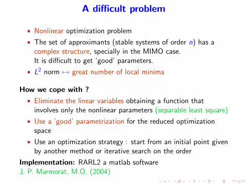
A difficult problem

• Nonlinear optimization problem

• The set of approximants (stable systems of order n) has acomplex structure, specially in the MIMO case.It is difficult to get ’good’ parameters.

• L2 norm 7→ great number of local minima

How we cope with ?

• Eliminate the linear variables obtaining a function thatinvolves only the nonlinear parameters (separable least square)

• Use a ’good’ parametrization for the reduced optimizationspace

• Use an optimization strategy : start from an initial point givenby another method or iterative search on the order

Implementation: RARL2 a matlab softwareJ. P. Marmorat, M.O. (2004)

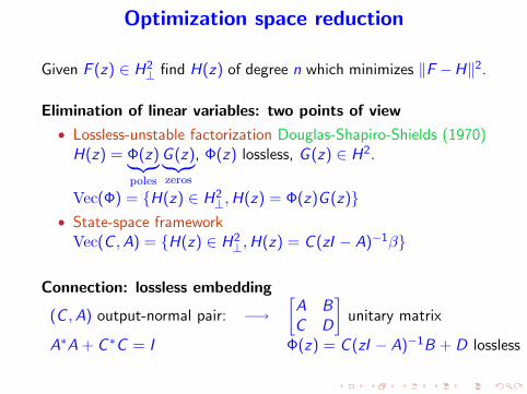
Optimization space reduction

Given F (z) ∈ H2⊥ find H(z) of degree n which minimizes ‖F −H‖2.

Elimination of linear variables: two points of view

• Lossless-unstable factorization Douglas-Shapiro-Shields (1970)H(z) = Φ(z)︸︷︷︸

poles

G (z)︸︷︷︸zeros

, Φ(z) lossless, G (z) ∈ H2.

Vec(Φ) = H(z) ∈ H2⊥,H(z) = Φ(z)G (z)

• State-space frameworkVec(C ,A) = H(z) ∈ H2

⊥,H(z) = C (zI − A)−1β

Connection: lossless embedding

(C ,A) output-normal pair: −→[A BC D

]unitary matrix

A∗A + C ∗C = I Φ(z) = C (zI − A)−1B + D lossless

The concentrated criterion

The projection theorem (orthogonality principle) in a Hilbert spaceallows to compute

• G (z) from Φ(z)

• β from (C ,A)

Concentrated criterion

J(C ,A) = minH∈Vec(C ,A)

‖F − H‖2

Advantages:

• The dimension of the parameter space is reduced but we alsoget a better-conditioned problem

• Lossless matrices enter the picture (transfer functions ofconservative systems)

Which parametrizations for lossless systems?

• An atlas of local coordinate maps: identifiability,differentiability

• Parametrizations with a double interpretation• Schur analysis and interpolation theory

A nice way to address the constraint metric ‖F‖∞ ≤ 1.Big inpact in system theory.Kailath (1986), Kimura, Ball, Gohberg and Rodman (1990)

• Balanced state-space canonical formsUseful in computations; physical interpretation

Hanzon, M.O., Peeters, LAA (2006),Marmorat, M.O., Automatica(2007)

Optimization process in RARL2

G0

G

0G0

VG

0

• V 7→ G (z) =

(A BC D

)computed from V and G0 as a

product of two unitary matrices (well-conditionned)

• Optimization with respect to local coordinates V (fmincon)Nonlinear condition reached → change of chart

• Nonlinear condition: eig min Q ≥ ε where Q is the solution toQ − A∗QA0 = C ∗C0.

Plan




Identification of hyperfrequency filters

• Electro-magnetic waves filter made of resonant cavities,interconnected by coupling irises (orthogonal double slits).Each cavity has 3 screws.

• Works around the GHz, Passband: a few Mhz

• Used in space telecommunication (satellites transmission) formultiplexing purposes.

Identification problem: given measurements performed on thedevice find the values of parameters from the physical modelWhat for ? Tuning (adjusting the screws)

An equivalent electrical model (1)

• Maxwell equations

• Input and output : one spacial mode (waveguide)electric field ≈ voltage

magnetic field ≈ currentThe filter can be seen as a quadripole, with two ports.

• The electrical field in each cavity is decomposed along twoorthogonal modes (approximation valid in the range offrequencies)

• For each mode, a good approximation of the Maxwellequations is given by the solution of a second order differentialequation.One mode in one cavity 7→ a RLC circuit (order 2)

An equivalent electrical model (2)

Screws act as capacitorsIrises results in a coupling between two horizontal (or two vertical)modes of adjacent cavitiesOrder = 2× 9 (two times the number of modes)

Low-pass equivalent electrical model

Original filter: two (conjugate) bandwidths in the high frequencies↓ low-pass transformation

Low-pass equivalent : one bandwidth around 0

one mode = one circuit (order 1)order = number of modesMi ,j coupling

State-space representation

We are interested in the power which is transmitted and reflected.

x(t) = Ax(t) + Ba(t)b(t) = Cx(t) + a(t)

a(t) =

[a1(t)a2(t)

]b(t) =

[b1(t)b2(t)

]Scattering matrix: S(z) = I + C (zI − A)−1Blossless symmetric with complex coefficients

C =

[j√

2R1 0 · · · · · · 00 · · · · · · 0 j

√2R2

]B = C t

A = −R − jM, A = At 2R = −C tC

M coupling matrix

Identification vs Model Reduction

-

completion

-

reduction

•

•••

•

•

•

••

H(iωk) H(s)H(s)

frequency data stable model rational model

A difficult problem:

→ Interpolate and extrapolate the data (band-limited)

→ Ensure stability

→ Find a small order model

Resolution in 3 steps

• Interpolation/extrapolation of the frequency datadedicated method

• Model reduction by rational L2-approximation RARL2

• Computation of the physical parameters from a realizationin a particular form (coupling matrix) DEDALE (F.Seyfert)

Presto-HF (F. Seyfert) is a matlab based toolbox dedicated tothe identification problem of low pass coupling parameters ofband pass microwave filters. Used by CNES, IRCOM, Alcatel.

Numerical results

The future

Omux identification and design

Plan




Inverse EEG (electroencephalography)problem

From measurements by electrodes of the electric potential u on thescalp, recover a distribution of m pointwise dipolar current sourcesCk with moments pk located in the brain (modeling the presenceof epileptic foci).L. Baratchart, M. Clerc, J. Leblond, J.P. Marmorat, M. Zghal

Mathematical model

The head Ω is modeled as aset of 3 spherical nested re-gions Ωi ⊂ R3, i = 0, 1, 2(brain, skull, scalp), with piece-wise constant conductivity σi ,separated by interfaces Si .

Macroscopic model + quasi-static approximation of Maxwellequations→ Spatial behavior of u in Ω

(P)

div (σ∇u) =m∑

k=1

pk .∇δCkin Ω

u = and ∂nu given on ∂Ω

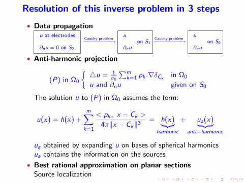
Resolution of this inverse problem in 3 steps

• Data propagationu at electrodes

∂nu = 0 on S2

Cauchy problem−−−−−−−−−→u

∂nuon S1

Cauchy problem−−−−−−−−−→u

∂nuon S0

• Anti-harmonic projection

(P) in Ω0

4u = 1

σ0

∑mk=1 pk .∇δCk

in Ω0

u and ∂nu given on S0

The solution u to (P) in Ω0 assumes the form:

u(x) = h(x) +m∑

k=1

< pk , x − Ck >

4π‖x − Ck‖3= h(x)︸︷︷︸

harmonic

+ ua(x)︸︷︷︸anti−harmonic

ua obtained by expanding u on bases of spherical harmonicsua contains the information on the sources

• Best rational approximation on planar sectionsSource localization

Best rational approximation on planar sections

• Slice Ω0 along a family of planes Πp:Πp ∩ Ω0 = Γp (disks) Πp ∩ S0 = Γp (circles)

• From pointwise values on Γp, compute the best L2 rationalapproximation to fp = (ua|Γp )2 on Γp

Why does it works ?

2 sources above view

• fp is a (meromorphic) function whose singularities ζk, p insideDp are strongly and explicitely linked with the sources Ck .

• (ζk, p) are aligned together and also with the complexcoordinates ζk of Ck .

• |ζk, p| is maximum at ζk, p = ζk (the k th source’s section)

• The poles ζk, p of the best L2 rational approximation to fp onΓp accumulate to the singularities ζk,pLeblond, Baratchart, Yattselev

FindSource3D

viewof u on S2 then of C1 into Ω0

R. Bassila, M. Clerc, J. Leblond, J.P. Marmorat

Plan




Wavelets in analog circuits

The continuous-time wavelet transform of a signal f (t)

Wψ(τ, σ) =1

σ

∫f (t)ψ

(t − τσ

)dt

• Widely used signal processing technique in medicalapplications (cardiac signal processing)

• Provides combined time and frequency localization

Can be implemented with a linear system:

f ∗ h(t) =

∫f (τ)h(t − τ) dτ, h(t) =

1

σψ

(−t

σ

)Only the implementation of strictly causal stable filters is feasible !To ensure causality, a time-shifted (truncated) time-reversedmother wavelet ψ(t) = ψ(t0 − t) is considered.

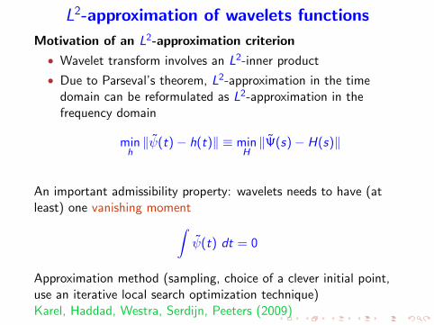
L2-approximation of wavelets functions

Motivation of an L2-approximation criterion

• Wavelet transform involves an L2-inner product

• Due to Parseval’s theorem, L2-approximation in the timedomain can be reformulated as L2-approximation in thefrequency domain

minh‖ψ(t)− h(t)‖ ≡ min

H‖Ψ(s)− H(s)‖

An important admissibility property: wavelets needs to have (atleast) one vanishing moment∫

ψ(t) dt = 0

Approximation method (sampling, choice of a clever initial point,use an iterative local search optimization technique)Karel, Haddad, Westra, Serdijn, Peeters (2009)

Model reduction using RARL2

• The given function F (z): the approximation obtained by Karel& al. converted into a discrete-time transfer function.

• The vanishing moment condition yields on the discrete-timeapproximant H(z) = C (zI − A)−1β the linear condition on β

C (I + A)−1β = 0

• It can be handled by a slightly different concentrated criterion

J(A,C ) = minβ ‖F (z)− H(z)‖2

subject to C (I + A)−1β = 0

β is easily computed from A and C using Lagrangemultipliers. Same optimization space and parametrization.

• Incremental search on the order

Approximation of Morlet wavelet

Initial approximation order 20 / RARL2 approximation order 8

Approximation of DB7 wavelet


Approximation of DB3 wavelet


Perspectives

• Convex constraints on the approximant can be handled withthe same optimization space (output normal pairs)

→ Vanishing moments (wavelets)→ Positive real, bounded real (β solution to an LMI)

• The same optimization space can be used for other criterions(separable least-square)RARL2 subroutines divides into two independant libraries :arl2lib: computation of the concentrated criterion, gradientwith respect to A,Cboplib: parametrization of balanced output pairs C ,A

→ Multi-objective control (β solution to an LMI Scherer)→ (weighted) Nonlinear least-square

http://www-sop.inria.fr/apics/RARL2/rarl2-eng.html

L2 Rational Approximation, Model Reduction and … Rational Approximation, Model Reduction and ......

Documents

Transcript of L2 Rational Approximation, Model Reduction and … Rational Approximation, Model Reduction and ......