L10. 　 Agent Negotiations

• When

• Definition and concepts

• Strategies – negotiation modeling

• Examples – a buyer-seller negotiation

When negotiations occur?

• Task and resource allocation

• Recognition of conflicts

• Improved coherence for agent society

• Deciding Organizational Structure

Definitions of Negotiation

• Davis&Smith

Negotiation is a process of improving agreement (reducing inconsistency and uncertainty) on common viewpoint or plans through the exchange of relevant information

1. Two-way exchange of information (e.g. 2 agents)

2. Individual perspective evaluation of information

3. Possible final agreement

Related Elements

• Negotiation – three main structures1. Language

2. Decision

3. Process

ProcessL

ang

uag

e

Decision

NEGOTIATION

PROCESS

Process

Lan

gu

age

Decision

Com

plet

ers

Reactors

Initiators

Primitives

Offers/tasks Plans

Context

Object Structure

Action Sequences Protocols

Modal LogicEffect

Pre-conditions Semantics

Conflict

Resolution

Cycle

Neg

otiatio

n

Cycle

Procedure

Matching Preferen

ces

Strategies

NEGOTIATION

Gra

mm

ar

Utility

Game Theory

Decision

Matrixes

Opt

imiz

atio

n

Probl

em

Non-C

onflicting

Plans

Max. Gain Min. Risk

Fair Solution

(50-50)

Con

cede

Uni

late

rally

Competetive

CooperativeInactionB

reak

ing

Beh

avior

Total Work (TW)

Live

ness

/Fai

rnes

s

Negotiation Problem Domains

Three-level hierarchy

1. Task-Oriented– Non-conflicting jobs/tasks

– Jobs/tasks can be redistributed among agents (for mutual benefit)

2. State-Oriented• Superset of task-oriented domain

• Goals/jobs/tasks can have side-effects (i.e. Conflicting)

• Negotiation joint plans/schedules for agents

3. Worth-Oriented• Superset of state-oriented domain

• Each goal has a rating or value (e.g. Numeric)

• Negotiation joint plans/schedules/goal relaxation

Postmen Problem

Domain Type: task-oriented

Situation:

• Several postmen located at a post office

• Post arrives to the post office

• Post is supposed to be delivered by the postmen to private postal boxes which is geographically (spatially) distributed

• Which postman should deliver which post to where?

Postmen Domain

Post OfficePost Office

a

c

d e

21

TODTOD

b

f

Blocks World Problem

Domain Type: state-oriented

Situation: agents have their own agenda on how to stack various colored blocks. Blocks are a shared resource.

How to coordinate the agents actions to solve conflicting block moves?

Slotted Blocks World

11 22 33

11 22 33

SODSOD

2

1

Multiagent Tile World Problem

Domain Type: worth-oriented

Situation: agents operate on a grid, there are tiles that needs to be put into holes. The different holes have different values. In addition there are obstacles.

How to coordinate the agents actions to solve conflicting tile-moves and get good compromises regarding the agents obtained values?

The Multi-Agent Tileworld

2 22

2

55

34

AB tilehole

obstacle

agents

WODWOD

Building Blocks

• Domain– A precise definition of what a goal is– Agent operations

• Negotiation protocol– A definition of a deal– A definition of utility– A definition of the conflict deal

• Negotiation Strategy– In Equilibrium– Incentive-compatible

Task-Oriented Domain – formal description

• Described by a tuple - <T, A, c>

• T – set of all tasks (all possible actions in the domain)

• A – list of agents

• c – a monotonic cost function for each task to a real number

Possible Deals

1. ({a}, {b})

2. ({b}, {a})

3. ({a, b}, )

4. (, {a, b})

5. ({a}, {a, b})

6. ({b}, {a, b})

7. ({a, b}, {a})

8. ({a, b}, {b})

9. ({a, b}, {a, b})

The conflict deal

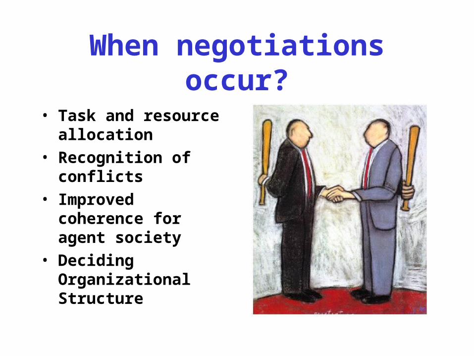
Formal Description of a ”Deal”

A deal is a pair (D1, D2) such that:

D1 D2 = T1 T2

T1 – Agent 1’s original task

T2 – Agent 2’s original task

D1 – Agent 1’s new task – result of deal

D2 – Agent 2’s new task – result of deal

Utility Function

Given encounter <T1, T2>, the utility of deal to

agent k is:utilityk() = c(Tk) – costk()

• = <D1, D2>

• c(Tk) is the stand-alone cost to agent k (the cost of achieving its goal with no help)

• costk() = c(Dk)

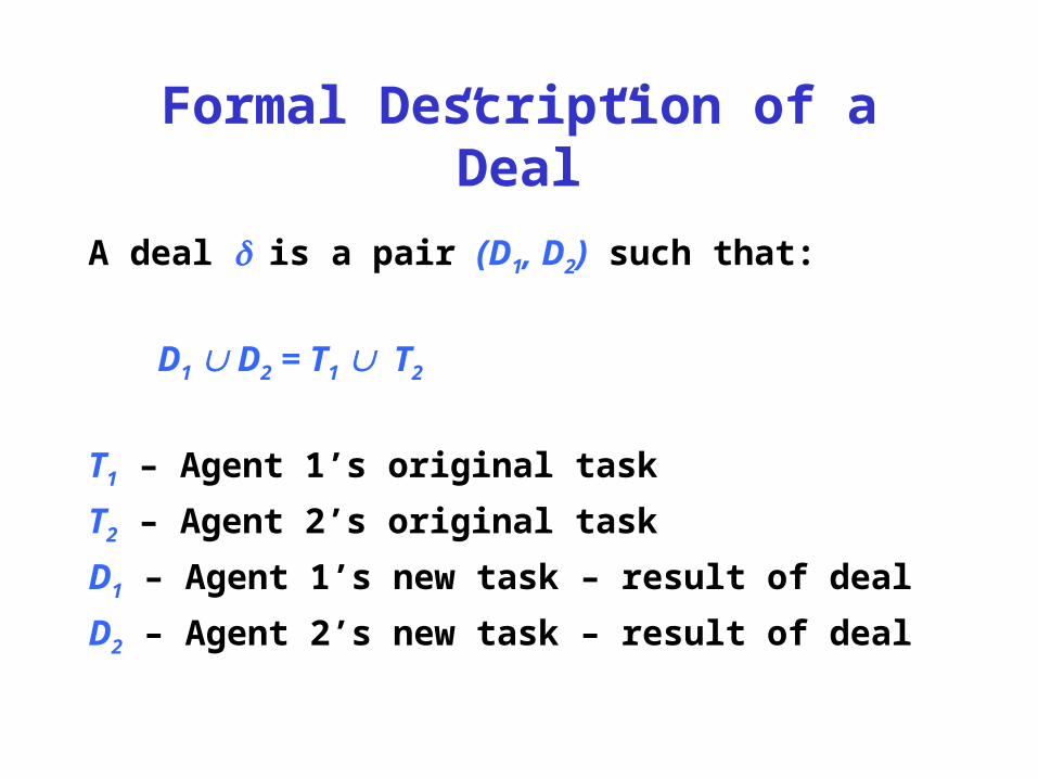
Example: parcel delivery domain -- utility

1 1

distribution point

a b

Utility for agent 1:

1. utility1({a}, {b}) = 0

2. utility1({b}, {a}) = 0

3. utility1({a, b}, ) = -2

4. utility1(, {a, b}) = 1

5. utility1({a}, {a, b}) = 0

6. utility1({b}, {a, b}) = 0

7. utility1({a, b}, {a}) = -2

8. utility1({a, b}, {b}) = -2

9. utility1({a, b}, {a, b}) = -2

Utility for agent 2:

1. utility2({a}, {b}) = 2

2. utility2({b}, {a}) = 2

3. utility2({a, b}, ) = 3

4. utility2(, {a, b}) = 0

5. utility2({a}, {a, b}) = 0

6. utility2({b}, {a, b}) = 0

7. utility2({a, b}, {a}) = 2

8. utility2({a, b}, {b}) = 2

9. utility2({a, b}, {a, b}) = 0

Cost function:

c() = 0

c({a}) = 1

c({b}) = 1

c({a,b}) = 3

Deals

1. ({a}, {b})

2. ({b}, {a})

3. ({a, b}, )

4. (, {a, b})

5. ({a}, {a, b})

6. ({b}, {a, b})

7. ({a, b}, {a})

8. ({a, b}, {b})

9. ({a, b}, {a, b})

({a}, {b})

({b}, {a})

(, {a, b})

({a}, {a, b})

({b}, {a, b})

({a}, {b})

({b}, {a})

({a, b}, )

(, {a, b})

Invidual rational

Pareto optimal

({a}, {b})

({b}, {a})

(, {a, b})

Negotiation sets

The Negotiation Set Illustrated

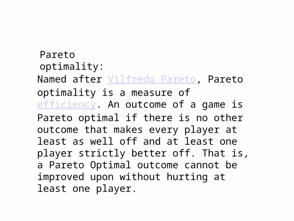
Named after Vilfredo Pareto, Pareto optimality is a measure of efficiency. An outcome of a game is Pareto optimal if there is no other outcome that makes every player at least as well off and at least one player strictly better off. That is, a Pareto Optimal outcome cannot be improved upon without hurting at least one player.

Pareto optimality:

Negotiation Protocols

• Agents use a product-maximizing negotiation protocol (as in Nash bargaining theory)

• It should be a symmetric PMM (product maximizing mechanism)

• Examples: 1-step protocol, monotonic concession protocol…

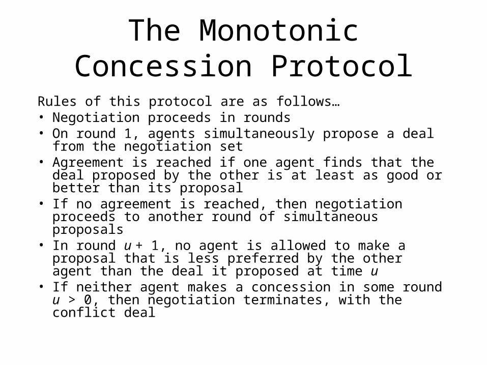
The Monotonic Concession Protocol

Rules of this protocol are as follows…• Negotiation proceeds in rounds• On round 1, agents simultaneously propose a deal from the

negotiation set• Agreement is reached if one agent finds that the deal

proposed by the other is at least as good or better than its proposal

• If no agreement is reached, then negotiation proceeds to another round of simultaneous proposals

• In round u + 1, no agent is allowed to make a proposal that is less preferred by the other agent than the deal it proposed at time u

• If neither agent makes a concession in some roundu > 0, then negotiation terminates, with the conflict deal

The Zeuthen Strategy

Three problems:

• What should an agent’s first proposal be?Its most preferred deal

• On any given round, who should concede?The agent least willing to risk conflict

• If an agent concedes, then how much should it concede?Just enough to change the balance of risk

Willingness to Risk Conflict

• Suppose you have conceded a lot. Then:– Your proposal is now near the conflict deal– In case conflict occurs, you are not much worse off– You are more willing to risk confict

• An agent will be more willing to risk conflict if the difference in utility between its current proposal and the conflict deal is low

Nash Equilibrium Again…• The Zeuthen strategy is in Nash equilibrium: under the

assumption that one agent is using the strategy the other can do no better than use it himself…

• This is of particular interest to the designer of automated agents. It does away with any need for secrecy on the part of the programmer. An agent’s strategy can be publicly known, and no other agent designer can exploit the information by choosing a different strategy. In fact, it is desirable that the strategy be known, to avoid inadvertent conflicts.

A Nash equilibrium, named after John Nash, is a set of strategies, one for each player, such that no player has incentive to unilaterally change her action. Players are in equilibrium if a change in strategies by any one of them would lead that player to earn less than if she remained with her current strategy. For games in which players randomize (mixed strategies), the expected or average payoff must be at least as large as that obtainable by any other strategy.

Nash equilibrium:

•　base　on　the　original　Bazaar　model

•　take　wholesalers　into　considerations

•　use　game　theory　in　generating　initial　strategy　

•　combine　common&public　knowledge

A Hybrid Negotiation Model

Extended　bazaar　model　-　a　brief　description　

•　a　10-tuple,　<G,　W,　　D,　　S,　　A,　H,　Ω,　　P,　　C,　E>　　　　　　　–　G,　a　set　of　players

　　　　　　　　–　W,　a　set　of　wholesalers

　　　　　　–　D,　a　set　of　negotiation　issues

　　　　　　　　–　S,　a　set　of　agreements　over　each　issue

　　　　　　–　A,　a　set　of　all　possible　actions

　　　　　　　　–　H,　a　set　of　history　sequences

　　　　　　–　Ω,　a　set　of　relevant　information　entities

　　　　　　　　–　P,　a　set　of　subjective　probability　distribution

　　　　　　–　C,　a　set　of　communication　costs　

　　　　　　　　–　E,　a　set　of　evaluation　functions

Extended　bazaar　model　–　in　a　bilateral　case

•　a　10-tuple,　<G,　W,　　D,　　S,　　A,　H,　Ω,　　P,　　C,　E>　　　　　　　–　G,　a　seller　and　a　buyer

　　　　　　　　–　W,　a　wholesaler

　　　　　　–　D,　a　single　issue-product　price

　　　　　　　　–　S,　price　offer/counter　offer

　　　　　　–　A,　possible　price　offers/counter　offers

　　　　　　　　–　H,　a　sequence　of　price　offers/counter　offers　

　　　　　　　　　　　　　　　　at　each　negotiation　round,　

　　　　　　　　　　　　　　　　(ak|k=1,2,…,K H)∩(L<K) ⇒ (ak |k=1,2,…,LH)

(ak|k=1,2,…,K H)∩(aK{accept, quit})⇒ak {accept, quit}|k=1,2,…,K-1　

　　　　　　　　　　　　　　　　　　　　　　　　　　　　　　　　　　　　　–　continue　…

•　a　10-tuple,　<G,　W,　　D,　　S,　　A,　H,　Ω,　　P,　　C,　E>　　　　　　　–　Ω,　a　set　of　knowledge　entities　a　seller/buyer　has　

　　　　　　　　　　　　　　　　　about　environment　(average　price,　economic　situation,　…),

　　　　　　　　　　　　　　　　　　　　　　　　　　counter　party　(RP,　payoff　function,　type…)　　　　　　　　–　P,　subjective　probability　distribution　of　hypothesis　on　a　belief　x.

　　　　　　　　　　　　　　　P[h,1]　(x),　　　　P[h,2]　(x)

　　　　　　–　C,　communication　costs　for　a　seller　or　buyer　

　　　　　　　　　　　　　　　　to　continue　another　negotiation　round　

　　　　　　　　–　E,　Ei:　(P[i,　h]　(x)|xΩi,　Pfi,　a)　→　utility(gi),　aAi,　　EiE,　　

i=1,2

　　　　　　　　　　　　　　　　　　　　　　　　　　　　　　　　　　　　　–　continue　…

•　a　10-tuple,　<G,　W,　　D,　　S,　　A,　H,　Ω,　　P,　　C,　E>　

　　　　　　　　–　E,　two　evaluation　function,one　for　a　seller　and　one　for　

a　buyer.

　　　　　　　　　　　　　　　Ei:　(P[i,　h]　(x)|xΩi,　Pfi,　a)　→　utility(gi),　aAi,　　EiE,　　

i=1,2

　　　　　　　　　　　　　　　　For　any　action a,　it　falls　into　three　types:

　　　　　　　　　　　　　　　　　　　　Ui　=　1.0　->　{agreement:　　accept},　

　　　　　　　　　　　　　　　　　　　　Ui　=　0.0　->{agreement:　　quit},　and　

　　　　　　　　　　　　　　　　　　　　0.0　<　Ui　<　1.0　->{new　agreement　}

•　　Accept: 　 If　price(akseller)　<　RPbuyer,　then　E[1,　a

k]=1,　ak=accept

• Quit:　　If　(price(akseller)　–RPseller<=C1　)∩(price(ak

seller)　>RPbuyer),　

　　　　　then　E[1,　ak]=0,　ak=quit

• fitness: f1(skj)=1-(CPbuyer(j)-RPseller)/(RPbuyer-RPseller),　

　　　　　　　　　　　　　　RPbuyer-　　C1>CPbuyer(j)>RPseller　skj=CPbuyer(j)S1,　j=1,　2,

…,　Np　　　

　　　　　　　　　　　　　　　　　　　　skj0　is　selected　as　the　counter-offer　if　we　have　

　　　　　　　　　　　　　　　　　　f1(skj0)=max{　f1(s

kj)}　,　j0j　

•　　　skj0　=　RPseller+

　is　regarded　as　a　psychological　factor

　Making　a　decision　over　price　only

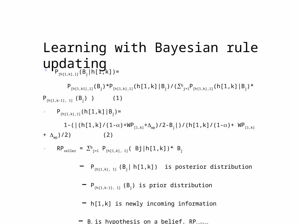
Learning　with　Bayesian　rule　updating•　P[h[1,k],1](Bj|h[1,k])=

　　　　　　　P[h[1,k1],1](Bj)*P[h[1,k],1](h[1,k]|Bj)/(bj=1P[h[1,k],1](h[1,k]|Bj)*　P[h[1,k-1],　1]　(Bj)　)　　　　

(1)　

•　　　P[h[1,k],1](h[1,k]|Bj)=

　　　　　　1-(|(h[1,k]/(1-)+WP[1,k]+wp)/2-Bj|)/(h[1,k]/(1-)+　WP[1,k]　+　wp)/2)　　　　　　　　　

(2)

• RPseller = bj=1 P[h[1,k], 1]( Bj|h[1,k])* Bj

　　　　　　–　P[h[1,k],　1]　(Bj|　h[1,k])　　is　posterior　distribution

　　　　　　　　　　　–　P[h[1,k-1],　1]　(Bj)　is　prior　distribution

　　　　　　　　　　　–　h[1,k]　is　newly　incoming　information

　　　　　　　　　　–　Bj　is　hypothesis　on　a　belief.　RPseller

　　　　　　　　

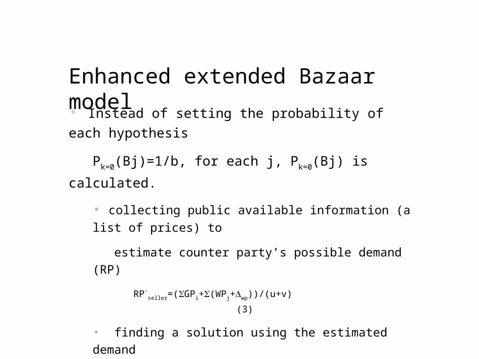
Enhanced　extended　Bazaar　model•　Instead　of　setting　the　probability　of　each　

hypothesis　　　　

　　　Pk=0(Bj)=1/b,　for　each　j,　Pk=0(Bj)　is　calculated.　

•　collecting　public　available　information　(a　list　of　

prices)　to　　

　　　estimate　counter　party’s　possible　demand　(RP)

　　　　　　　　　RP’seller=(GPi+(WPj+wp))/(u+v)　　　　　　　　　　　　　　　　　　　　　　　　　　　　　　　　　　　　　　　　　　　　　　　　　　　　　

(3)　

•　　finding　a　solution　using　the　estimated　demand

　　　　max(RPbuyer-x)(x-RP’seller),　　x　=　(RPbuyer+　RP’seller)/2　　　　　　　　　　　　　　　　　　　　　　　　　　　　　　

(4)

•　　initiating　the　probability　distribution

　　　　P’(Bj)　=　1-|x-Bj|/x　　　　　　　　　　　　　　　　　　　　　　　　　　　　　　　　　　　　　　　　　　　　　　　　　　　　　　　　　　　　　　　　　　　　　　　　　　　

(5)

　　　　Pk=0(Bj)　=　P’(Bj)/　P’(Bj)　　　　　　　　　　　　　　　　　　　　　　　　　　　　　　　　　　　　　　　　　　　　　　　　　　　　　　　　　　　　　　　　　　(6)

Updating　probability　distribution

 K

 Offer

Counter Offer

P(B1) P(B2) P(B3) P(B)

0 --- --- 0.17 0.26 0.33 0.24

1 140 107.9 0.16 0.22 0.29 0.33

2 135 109.7 0. 07 0.18 0.46 0.29

3 130 110.2 0.03 0.14 0.61 0.22

Enhanced Extended Bazaar

010203040506070

90 100 110 120hypotheses

prob

abili

ty(%

)

k=0k=1k=2k=3

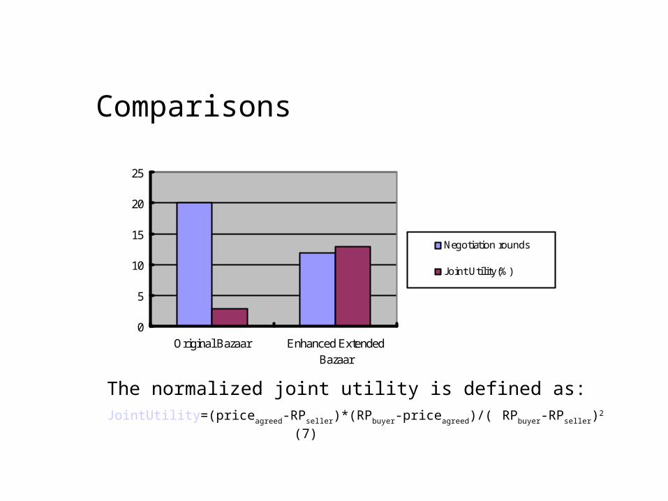
Comparisons

0

5

10

15

20

25

Original Bazaar Enhanced ExtendedBazaar

Negotiation rounds

Joint Utility(%)

The　normalized　joint　utility　is　defined　as:JointUtility=(priceagreed-RPseller)*(RPbuyer-priceagreed)/(　RPbuyer-RPseller)

2　　　　　　　　　　　　　　　　　　　　　　　　　　　(7)

　　　　　　　　　　　　　　　　　　　　　　　　　　　　　　　　　　　　　–　continue　…

O riginal Bazaar Based

0

50

100

150

200

250

300

1st 2nd 3rd 4th 5th 6th 7th 8th 9th 10throunds

pric

e

Seller

Buyer

RPseller

RPbuyer

Enhanced Extended Bazaar Based

0

50

100

150

200

250

300

1st 2nd 3rd 4th 5th 6th

rounds

pric

e

Seller

Buyer

RPseller

RPbuyer

System　configuration

…

Message Parser User Interface

Message Processing

Action Making

Internet

History Record Buyer Negotiation

Model

Buyer Agent

Internet

Message Parser User Interface

Message Processing

Action Making

Internet

History Record Seller Negotiation

Model

Seller Agent

Agent Data Holder

Agent Registration

Messenger

Agent server

proposal processing

proposal processing

A Real World Trading Oriented Market-driven Modelfor Negotiation Agent

Yoshizo Ishihara and Runhe Huang

Faculty of Computer and Information Sciences,Hosei University, Tokyo, Japan

Negotiation Agent

Bid

Bid

Seller

Buyer Seller　Agent

Buyer　Agent

Negotiation

Negotiation Factors

• Sim’s model is guided by following four negotiation factors:– Trading Opportunity– Trading Competition– Trading Time– Trading Eagerness of the agent itself

• The spread k’ between an agent’s bid/offer and that of others in the next trading cycle is determined as:

kEttTnmCvwnOk i )](),,',(),(),,(['

Our Improved Model

• We improved Sim’s model in 2004 using Bayesian updating rule to learn opponent’s eagerness.

• An agent can make a concession for its opponent’s motivation.

• The spread k’ is redefined as:

kEEttTnmCvwnOk ooaai )]()(),,',(),(),,(['

A Precondition

• In both Sim’s and our improved model, a negotiation agent has

same behaviors and actions

to all trading partners.

$800

$800

Same

A Real World Trading

• In fact, a negotiation strategy between a buyer and a seller is

kept in secret and unknown

to others.

????

????

Unknown

A Revised Model

• A revised market-driven model takes each trading partner as an individual with different strategies and actions.

$850

$750

Different　&　Unknown

The competition factor in the previous model

• Each trading partner hasa same number of competitors.

• Each seller getsa same number of demands.

• Each buyer getsa same number of supplies.

......

a[2] a[m]......

Item

b[2]

Item

b[n]

Item

Full　connected

b[1]

a[1]

Individual Competition (IC)

• A buyer requests i items.

• A seller has s supplies andsum(i) = d demands.

• is the probability that the buyer agent a will become supplied target for requested items from the seller agent b.

• If (s >= d), then

• If (s < d), then

id

isab

C

CIC

Item

1 abIC

abIC

ItemItem

.......ItemItemItem

b[1] b[n]

a[1] a[2] a[m].......

]1[]1[ bai ]1[]2[ bai

]1[]2[]1[]1[]1[ babab iid

]1[bs

Individual　connected

Apply to Conflict Probability

• IC = 1 do not affect to previous conflict probability.

• Lower IC makes higher conflict probability.

• IC = 0 makes conflict probability as 1.

ajtaja

t

ajt

jatja

tc ICcv

wvP

)1(1,

10

1

0 IC

Pc

Previous　ValueSupply

DemandDemand

DemandDemand

ex)　Higher　demands　make　higher　IC.

Individual Opportunity (IO)

• Learnt opponent eagerness, , will affect to opportunity.

• The probability that buyer agent a will obtain a utility v, with seller agent b:

– If Pc = 0.0 : Pc -> 0.001

– If Pc < 0.5 :

– If Pc = 0.5 :

– If Pc > 0.5 :

– If Pc = 1.0 : Pc -> 0.999

batIO

]1[log 5.0 PcbatIO

][log 5.0)1(1 PcbatIO

Revised Negotiation Strategy

• To bring close up to ,the agent makes an amount of concessionbased on the time-dependent strategy:

– when

– when

batIO ba

tIO '

bat

bat IOIO '

bat

bat IOIO '

)'(),,(),,( bat

bat

bababat IOIOtTtTv

)'()),,(1(),,( bat

bat

bababat IOIOtTtTv

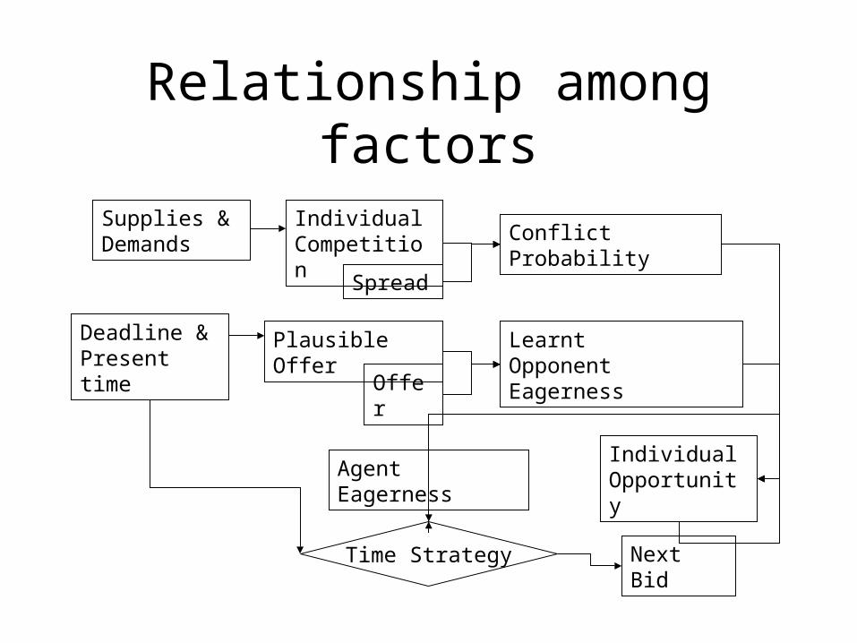
Relationship among factors

IndividualCompetition

Supplies　&　Demands

IndividualOpportunity

Conflict　Probability

Spread

Plausible　OfferDeadline　&　Present　time

LearntOpponent　Eagerness

Offer

Agent　Eagerness

Time　Strategy Next　Bid

Negotiation ResultsEach value shows:Bid　PriceLearnt　Opponent　EagernessIndividual　Opportunity

Negotiation ResultsEach value shows:Bid　PriceLearnt　Opponent　EagernessIndividual　Opportunity

References:

http://www.csc.liv.ac.uk/~mjw/pubs/gdn2001.pdf

http://www.ecs.soton.ac.uk/~mml/papers/ker99-2.pdf

http://crpit.com/confpapers/CRPITV4Rahwan.pdf

http://xenia.media.mit.edu/~guttman/research/pubs/amet98.pdf

http://www.umiacs.umd.edu/users/sarit/Articles/acai01.pdf

http://www-agki.tzi.de/ecai00-mas/lopes.pdf