RADAR Imaging Satellite (RISAT) 1 - Vienna International Centre

ESA Summer School 2006
L1 – Satellite radar
Andrew ShepherdUniversity of Edinburgh
Satellite radar – 21st century glaciology
ESA Summer School 2006
L1 – Satellite radar
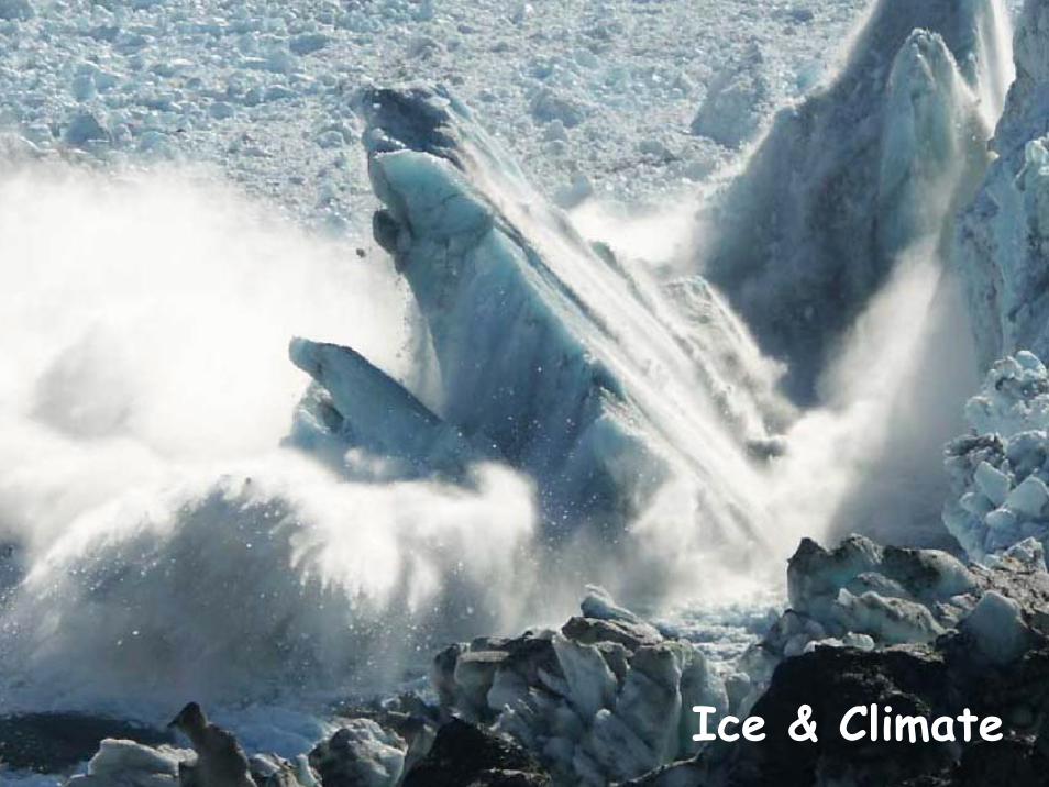
Ice & Climate

ESA Summer School 2006
L1 – Satellite radar
Planet Earth is characterised by the presence of water. In frozen form, snow and ice cover about a sixth of Earth’s surface.
This lecture provides an introduction to Earth’s crysophere, and explains why satellite radar is the modern tool for glaciologists.
Ice & climate

ESA Summer School 2006
L1 – Satellite radar
The cryosphere includes all frozen regions of the Earth, such as the polar ice sheets, mountain glaciers, floating sea ice, and the Arctic tundra. It is an important component of the Earth’s climate system, because ice is sensitive to changes in temperature such as thosethat have been predicted for the near future.
Icebergs
Permafrost
River & Lake Ice
Sea ice
Ice Shelves
Ice Sheets
Ice caps
Mountain Glaciers
Snow
Ice & climate

ESA Summer School 2006
L1 – Satellite radar
Frozen regions help us to study climate change in two key ways.
Firstly, sub-polar components of the cryosphere (e.g. alpine glaciers) are expected to respond quickly to changes in climate,and their progress can be used as a barometer for climate change predictions.
IntroductionIce & climate

ESA Summer School 2006
L1 – Satellite radar
Frozen regions help us to study climate change in two key ways.
Secondly, as climate change occurs, the quantity of water frozenwithin the cryosphere changes too, causing global sea levels to fluctuate.
IntroductionIce & climate

ESA Summer School 2006
L1 – Satellite radar
Today, water in solid phase exists on all of Earth’s continents at some time of the year.
IntroductionIce & climate

ESA Summer School 2006
L1 – Satellite radar
... although Africa’s ice is set to disappear in the next 20 years.
IntroductionIce & climate

ESA Summer School 2006
L1 – Satellite radar
Ice area is not a useful parameter for studies of climate change, because it is not generally related to mass.
For instance, when glaciers surge, their area can double, but their mass remains constant
IntroductionIce & climate

ESA Summer School 2006
L1 – Satellite radar
Ice volume, however, is directly related to mass through density, and so measuring changes in ice volume tells us directly how sea level is changing.
ρSNOW =350 kg m-3
ρFIRN =350-917 kg m-3
ρICE =917 kg m-3
IntroductionIce & climate

ESA Summer School 2006
L1 – Satellite radar
If all snow and ice above sea level were to melt, Earth’s continents would look very different.
IntroductionIce & climate

ESA Summer School 2006
L1 – Satellite radar
If all snow and ice above sea level were to melt, Earth’s continents would look very different.
IntroductionIce & climate

ESA Summer School 2006
L1 – Satellite radar
The vast majority of Earths ice is frozen in Antarctica
Introduction
0.1 m*
2 m*
0.01 m
0.6 m
~ 2 m
80 m
Volume (sea level equivalent)
14,000,000Ice Sheets
1,500,000Ice Shelves
33,000,000 Sea Ice
46,000,000Snow
5,000,000 Glaciers & Ice Caps
20,000,000 Permafrost
Area(km2)
Ice
Ice & climate
ESA Summer School 2006
L1 – Satellite radar
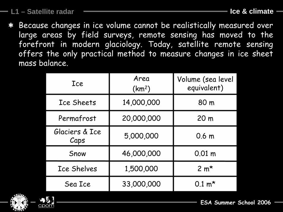
Because changes in ice volume cannot be realistically measured over large areas by field surveys, remote sensing has moved to the forefront in modern glaciology. Today, satellite remote sensing offers the only practical method to measure changes in ice sheetmass balance.
Introduction
0.1 m*
2 m*
0.01 m
0.6 m
20 m
80 m
Volume (sea level equivalent)
14,000,000Ice Sheets
1,500,000Ice Shelves
33,000,000 Sea Ice
46,000,000Snow
5,000,000 Glaciers & Ice Caps
20,000,000 Permafrost
Area(km2)
Ice
Ice & climate

ESA Summer School 2006
L1 – Satellite radar
Changes in ice sheet mass have moderated global sea level throughout the ice age. As Antarctica grows sea levels fall, as Antarctica shrinks sea levels rise.
Introduction
Measuring changes in ice sheet mass shows how much they contribute to present sea level change.
Ice & climate

ESA Summer School 2006
L1 – Satellite radar Introduction
Ice sheet mass can be measured in two ways:
Ice & climate
(1) By recording changes in total volume, and converting to mass.
(2) By recording the difference between mass input and output
Each approach requires measurements across entire ice sheets

ESA Summer School 2006
L1 – Satellite radar Introduction
(1) Volume change (whole ice sheet)
VTODAY = 26 x 106 km3
VLGM = 77 x 106 km3
ΔV = -51 x 106 km3
density = 917 kg m-3
ΔM = -47 x 106 GtΔM / Δt = -47 x 106 Gt / 21,000 yr
= -2200 tonne yr-1
360 Gt = 1 mm ESL
ΔESL / Δt = 6 mm yr-1
Ice & climate
ESA Summer School 2006
L1 – Satellite radar IntroductionIce & climate
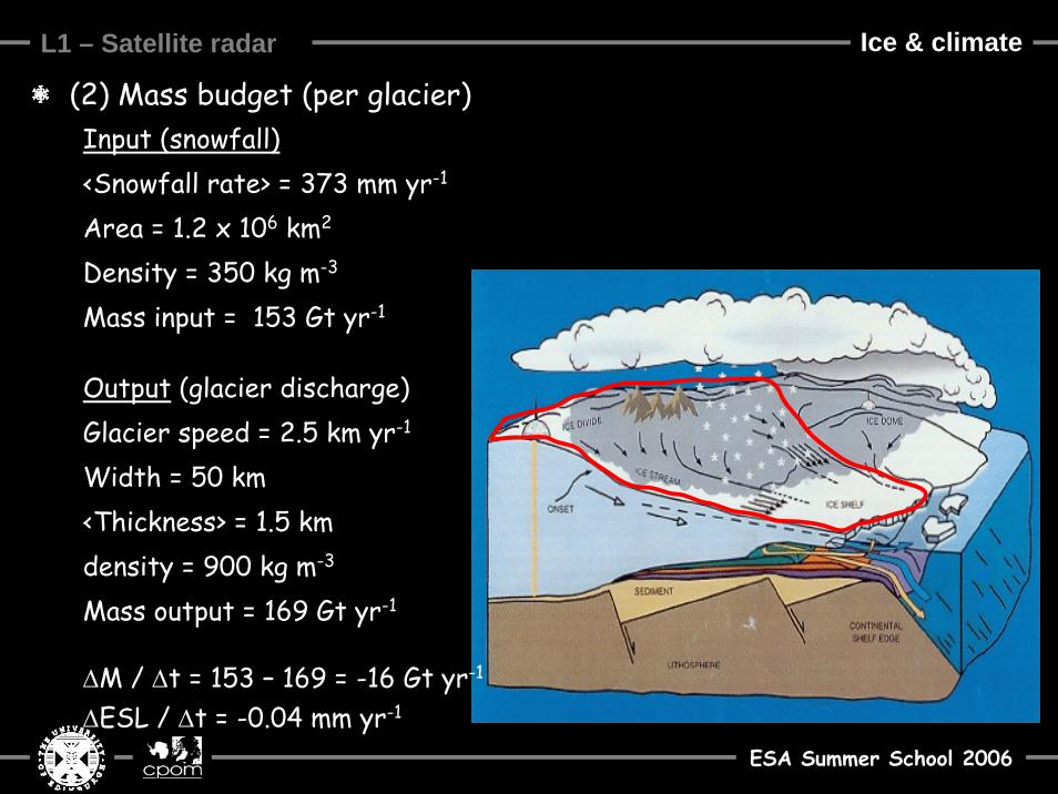
(2) Mass budget (per glacier)Input (snowfall)<Snowfall rate> = 373 mm yr-1
Area = 1.2 x 10⁶ km2
Density = 350 kg m-3
Mass input = 153 Gt yr-1
Output (glacier discharge)Glacier speed = 2.5 km yr-1
Width = 50 km<Thickness> = 1.5 kmdensity = 900 kg m-3
Mass output = 169 Gt yr-1
ΔM / Δt = 153 – 169 = -16 Gt yr-1
ΔESL / Δt = -0.04 mm yr-1

ESA Summer School 2006
L1 – Satellite radar
Observing Antarctica

ESA Summer School 2006
L1 – Satellite radar Observing Antarctica
1531: First map of Antarctica?

ESA Summer School 2006
L1 – Satellite radar Fieldwork
1882: First International Polar Year. The fundamental concept of the first IPY was that geophysical phenomena could not be surveyed by one nation alone; rather, an undertaking of this magnitude would require a global effort.
12 countries15 expeditions13 to the Arctic2 to the Antarctic

ESA Summer School 2006
L1 – Satellite radar
1914: Shackleton shipwrecks at Antarctic Peninsula
Observing Antarctica
ESA Summer School 2006
L1 – Satellite radar Fieldwork
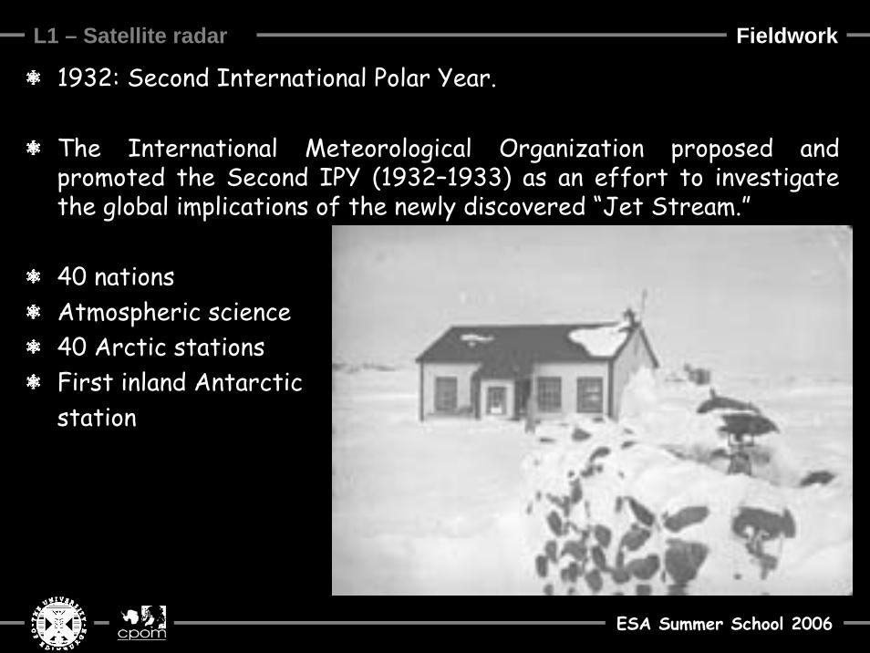
1932: Second International Polar Year.
The International Meteorological Organization proposed and promoted the Second IPY (1932–1933) as an effort to investigate the global implications of the newly discovered “Jet Stream.”
40 nations Atmospheric science40 Arctic stationsFirst inland Antarctic station
ESA Summer School 2006
L1 – Satellite radar
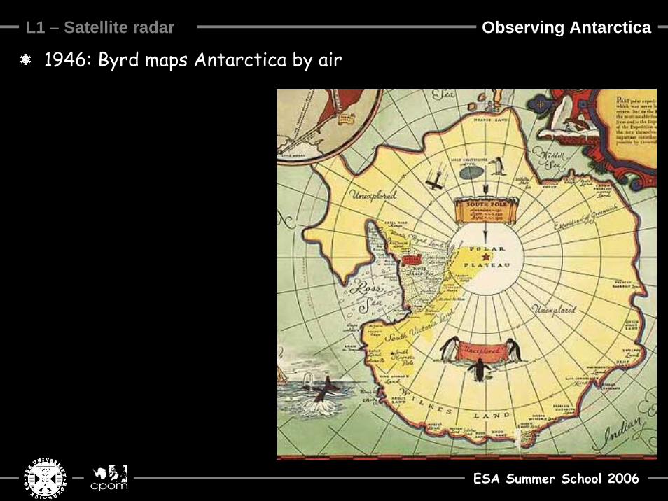
1946: Byrd maps Antarctica by air
Observing Antarctica

ESA Summer School 2006
L1 – Satellite radar Fieldwork
1957: The International Geophysical YearConceived to exploit technology developed during WWII (for example, rockets and radar)
Continental drift, confirmedFirst satellites launchedVan Allen Radiation Belt discoveredAntarctica’s ice mass quantifiedAntarctic Treaty ratified
ESA Summer School 2006
L1 – Satellite radar
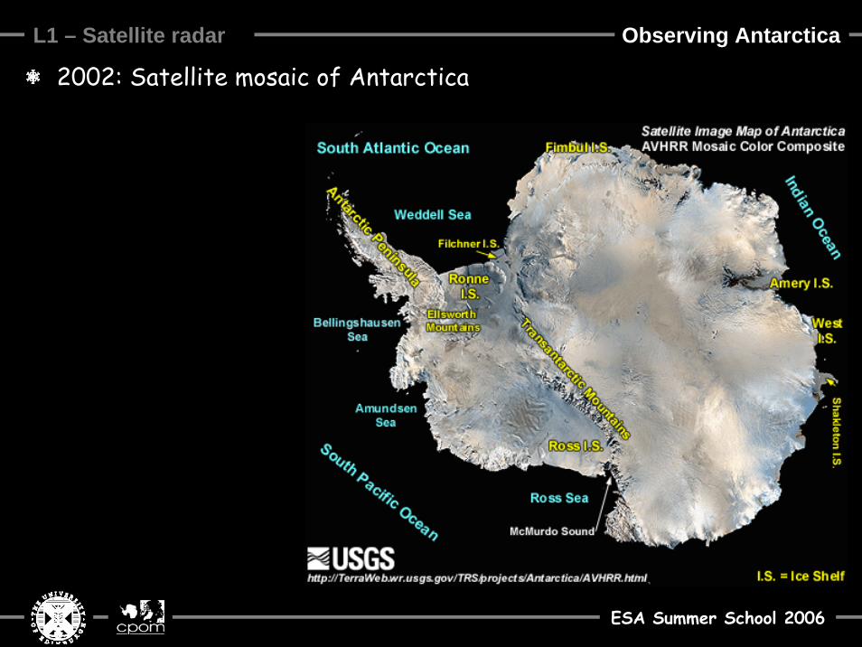
2002: Satellite mosaic of Antarctica
Observing Antarctica
ESA Summer School 2006
L1 – Satellite radar
2007: Third International Polar Year.IPY 2007 will expand upon the legacy of scientific achievement and societal benefits from past examples.
Observing Antarctica

ESA Summer School 2006
L1 – Satellite radar Observing Antarctica

ESA Summer School 2006
L1 – Satellite radar
Field sites visited since 1920’s
Observing Antarctica

ESA Summer School 2006
L1 – Satellite radar
Field stations occupied since 1940’s
Observing Antarctica
ESA Summer School 2006
L1 – Satellite radar
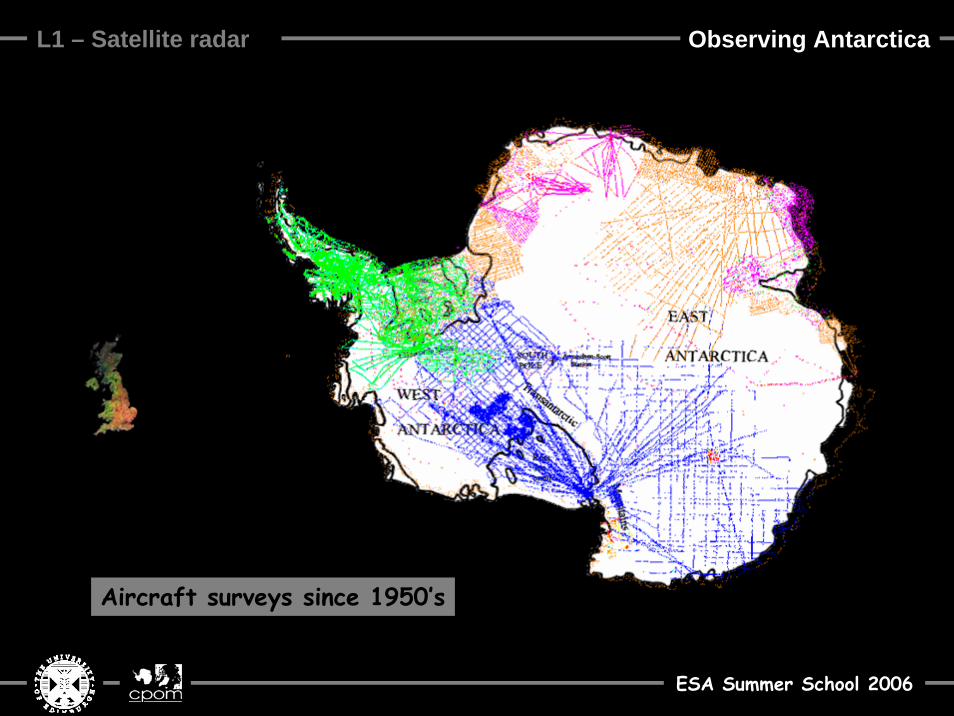
Aircraft surveys since 1950’s
Observing Antarctica
ESA Summer School 2006
L1 – Satellite radar
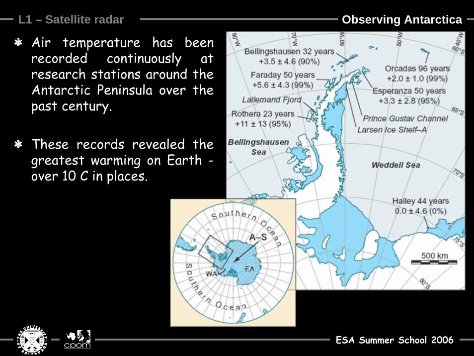
Air temperature has been recorded continuously at research stations around the Antarctic Peninsula over the past century.
These records revealed the greatest warming on Earth -over 10 C in places.
Observing Antarctica

ESA Summer School 2006
L1 – Satellite radar
Glaciological estimates of Antarctic mass balance (360 Gt = 1mm slr)
-40 ± 480
+48712621749Meir, 1983
+20018002000Budd, 1985
-46926132144Jacobs, 1992
19020102200Bentley, 1991
-720
+420
-400
Mass Balance(Gt)
2720
1660
2400
Mass output(Gt)
2000Kotlyakov, 1978
2080Bull, 1971
2000 Losev, 1963
Mass input(Gt)
Study
Observing Antarctica

ESA Summer School 2006
L1 – Satellite radar Satellite Remote Sensing
ESA Summer School 2006
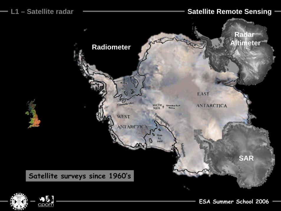
L1 – Satellite radar
Radiometer
SAR
Radar Altimeter
Satellite surveys since 1960’s
Satellite Remote Sensing

ESA Summer School 2006
L1 – Satellite radar
SAR
Radar Altimeter
Amundsen-Scott station, South Pole
Satellite surveys since 1960’s
Satellite Remote Sensing

ESA Summer School 2006
L1 – Satellite radar
The first satellites were cameras in space. They were placed in orbit before telecommunications were possible, and so their film had to be physically ejected down to Earth.
A C-119 aircraft recovers a film capsule ejected from the DMSP satellite program.
Satellite Remote Sensing

ESA Summer School 2006
L1 – Satellite radar
Modern instruments are far more sophisticated.
In 2009, the CryoSat-2 satellite will be launched, carrying an interferometric synthetic aperture radar altimeter
CryoSat-2 will record fluctuations in the volume of the polar ice sheets to a far greater precision than has been previously possible.
RADAR

ESA Summer School 2006
L1 – Satellite radar
Unlike photography, RADAR is a quantitative remote sensing technique. It can be used to measure distance and speed precisely
Oblique Photo Satellite composite
Satellite infrared Satellite radar
RADAR

ESA Summer School 2006
L1 – Satellite radar
Radio waves have the longest wavelengths (0.1 to 1000 m), followed by microwaves (0.1 to 100 mm), infrared, visible, UV and X-rays.
The Earth’s atmosphere (including clouds) is transparent to electromagnetic radiation with wavelengths from 1 mm to 20 m –which includes radio and microwaves. This is why TV and radio stations are able to broadcast over long distances.
RADAR
ESA Summer School 2006
L1 – Satellite radar
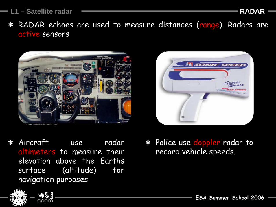
RADAR echoes are used to measure distances (range). Radars are active sensors
Aircraft use radar altimeters to measure their elevation above the Earths surface (altitude) for navigation purposes.
Police use doppler radar to record vehicle speeds.
RADAR

ESA Summer School 2006
L1 – Satellite radar
The principals of radar operation are straightforward, and are equally applicable to aircraft altimeters, satellite sensors and even police speed traps (not cameras).
R
Plan view
Side view(1) Radars transmit pulses of electromagnetic radiation at radio frequencies
(2) The radar pulse is scattered or reflectedby solid surfaces.
(3) The backscattered pulse (echo) is detected by the radar receiver
(4) The pulse travel time is recorded.
(5) The travel time is converted into the distance (range) separating the radar and the surface.
RADAR

ESA Summer School 2006
L1 – Satellite radar
The radar equation is very simple, and relates the travel time (T) to the distance travelled (range, R):
where c is the speed of light. Note the factor ½ to account for the fact that the radar pulse travels to the surface and back again in the time T.
cTR21
=
R
Plan view
Side view
RADAR

ESA Summer School 2006
L1 – Satellite radar
Altimeters are radars (e.g. on aircraft or satellites) pointed towards Earth to measure altitude.
Altimeters transmit a single pulse of electromagnetic radiation, and measure the range and power of the echo from one reflecting point
RADAR altimetry
ESA Summer School 2006
L1 – Satellite radar
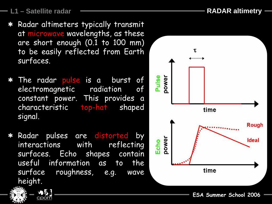
Radar altimeters typically transmit at microwave wavelengths, as these are short enough (0.1 to 100 mm) to be easily reflected from Earth surfaces.
The radar pulse is a burst of electromagnetic radiation of constant power. This provides a characteristic top-hat shaped signal.
Radar pulses are distorted by interactions with reflecting surfaces. Echo shapes contain useful information as to the surface roughness, e.g. wave height.
RADAR altimetry

ESA Summer School 2006
L1 – Satellite radar
Satellite altitude is precisely determined relative to the Earth’s geoid using gyroscopes to measure the gravity from space.
The geoid is a hypothetical reference level used to describe a surface close to mean sea level where the strength of gravity isconstant. Mountains are above the geoid, and sea floors are below.
RAh −=
Satellite altimeters can be used to measure the height of Earth’s surface relative to the geoid, for instance to create accurate digital elevation models (DEM’s).
The surface height (h) is simply the altitude (A) minus the radar range (R)
RADAR altimetry

ESA Summer School 2006
L1 – Satellite radar
Satellite radar altimeters are flown in near-polar orbits to repeatedly measure the Earth’s surface elevation. This allows us to determine surface height changes, such as ocean waves, lava flows, or ice sheet growth and decay.
Height change is determined at crossing points of the satellite orbit to allow for slight variations in the orbit trajectory, and for greater measurement precision.
Crossing point locations are closely spaced at high latitudes, where the orbits converge, and widely spaced at the equator.
RADAR altimetry

ESA Summer School 2006
L1 – Satellite radar
The European Remote Sensing (ERS-1 and ERS-2) satellites have the same radar altimeter onboard. ERS-1 was launched in 1991 and retired in 2000, ERS-2 was launched in 1995 still operates.
ERS orbits are inclined at 8° to the pole, fly at 782 km altitude, complete a single Earth revolution in 90 minutes, and principally follow 35 day repeat cycles.
ERS satellites have provided by far the most comprehensive dataset of ice sheet elevation change.
This includes 2/3 of the Antarctic ice sheet and the entire Greenland ice sheet, allowing precise estimates of their growth or decay and the resultant contribution to global sea level over the past decade.
RADAR altimetry

ESA Summer School 2006
L1 – Satellite radar RADAR altimetry
Wingham et al (1998) measured the volume change of 66% of the Antarctic ice sheet using ERS radar altimetry.
They calculated the ice sheet was losing 60 ± 76 Gt yr-1.
ESA Summer School 2006
L1 – Satellite radar
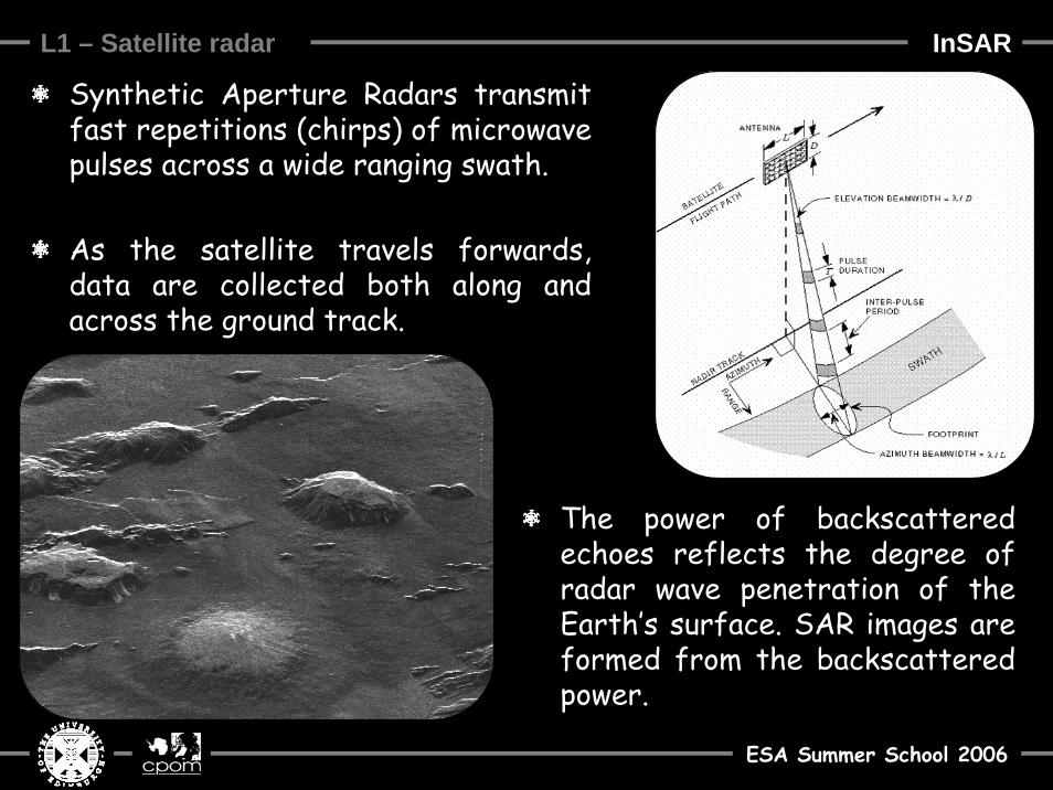
Synthetic Aperture Radars transmit fast repetitions (chirps) of microwave pulses across a wide ranging swath.
As the satellite travels forwards, data are collected both along and across the ground track.
The power of backscattered echoes reflects the degree of radar wave penetration of the Earth’s surface. SAR images are formed from the backscattered power.
InSAR

ESA Summer School 2006
L1 – Satellite radar
SAR uses an active source of illumination, and so images can be obtained at night.
SAR operates at microwave frequencies, and so images can be recorded through clouds.
SAR instruments look sideways, and so raw images appear skewed.
Side-looking SAR sensors cannot view areas of steeply sloping terrain (> 24�) that fall in the radar beam shadow.
InSAR
ESA Summer School 2006
L1 – Satellite radar
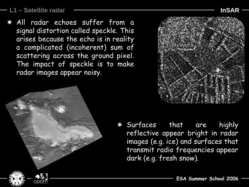
All radar echoes suffer from a signal distortion called speckle. This arises because the echo is in reality a complicated (incoherent) sum of scattering across the ground pixel. The impact of speckle is to make radar images appear noisy.
Surfaces that are highly reflective appear bright in radar images (e.g. ice) and surfaces that transmit radio frequencies appear dark (e.g. fresh snow).
RADAInSAR
ESA Summer School 2006
L1 – Satellite radar
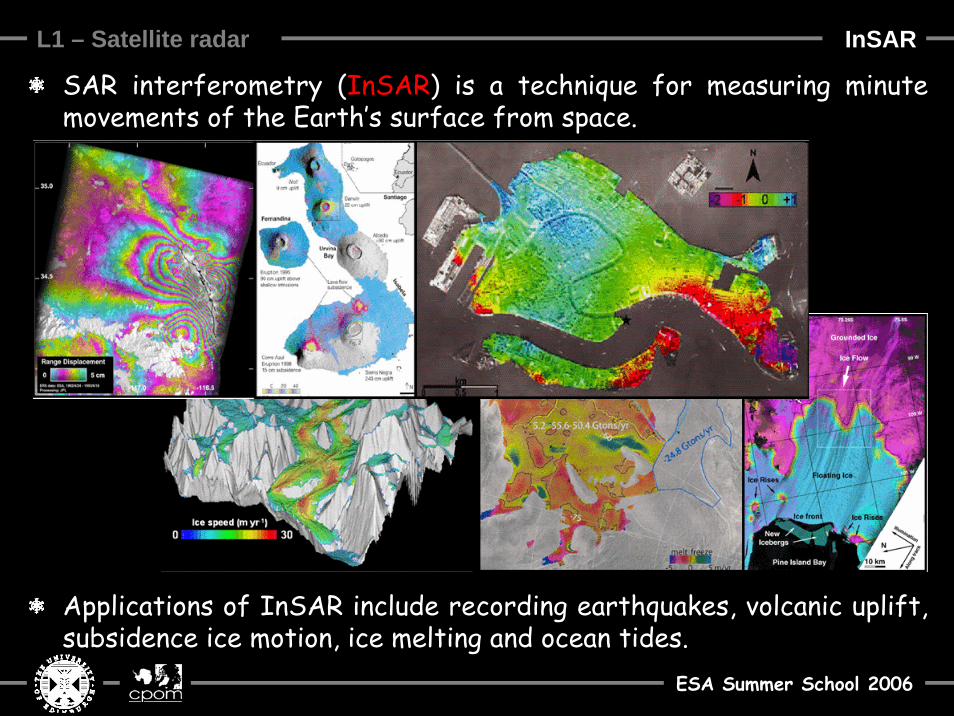
SAR interferometry (InSAR) is a technique for measuring minute movements of the Earth’s surface from space.
Applications of InSAR include recording earthquakes, volcanic uplift, subsidence ice motion, ice melting and ocean tides.
InSAR

ESA Summer School 2006
L1 – Satellite radar
The principal of InSAR is that two SAR images of the same area taken at separate times can be combined to produce an interference pattern (interferogram) related to surface movement and elevationduring the time interval.
The interference pattern arises due to the difference in radar range to each reflecting point between images.
This difference is expressed as a phase angle (0 to 360°), equal to the fraction of a complete radar wavelength.
SAR Image 1SAR Image 2
Interferogram
InSAR

ESA Summer School 2006
L1 – Satellite radar
The range difference (ΔR) can arise in two ways: (1) The satellite does not return to the same location on repeat(2) The surface can move during the intervening period.
(1) (2)
InSAR

ESA Summer School 2006
L1 – Satellite radar
πλφλ
πφλ
4221
21
=××==Δ NR
The range difference (ΔR) is related to the interferogram phase (φ) using the interferogram equation:
where N is the number of wavelengths within the range difference and λ is the radar wavelength (5.6 cm for ERS).
ΔR can then be partitioned into components due to surface topography (ΔRT) and motion(ΔRM) :
)(4
MTMT RRR φφπλ
+=Δ+Δ=Δ
InSAR

ESA Summer School 2006
L1 – Satellite radar
Elevation contours
Motion contours
Ice cap interferogram is a mixture of motion and
elevation contours
πλφλ
πφλ
4221
21
=××==Δ NR
The range difference (ΔR) is related to the interferogram phase (φ) using the interferogram equation:
where N is the number of wavelengths within the range difference and λ is the radar wavelength (5.6 cm for ERS).
ΔR can then be partitioned into components due to surface topography (ΔRT) and motion(ΔRM) :
)(4
MTMT RRR φφπλ
+=Δ+Δ=Δ
InSAR

ESA Summer School 2006
L1 – Satellite radar
The topographic phase φT can be calculated from the satellite orbitsand a digital elevation model (DEM) of the surface.
Orbits
DEM
Simulated topographic phase (φT) has elevation contours only
InSAR

ESA Summer School 2006
L1 – Satellite radar
Range due to surface motion is calculated by subtracting simulated topographic phase from an interferogram:
)(44
TMMR φφπλφ
πλ
−=Δ =
Interferogram (φ) Topographic phase (φT) Motion phase (φM)
)(44
TMMR φφπλφ
πλ
−=Δ =
InSAR

ESA Summer School 2006
L1 – Satellite radar
The range difference due to motion (ΔRM) can be converted into horizontal motion using the surface slope (β) using trigonometry:
Tsv M
SURF ΔΔ
==time
distance
θcosMM Rx Δ=Δ
βcosM
Mxs Δ
=Δ
βπθφφλ
cos4cos)(
Tv T
SURF Δ−
=
The horizontal component of ΔRM is
The surface plane component of ΔRM is
The surface plane velocity is
and so
InSAR
ESA Summer School 2006
L1 – Satellite radar
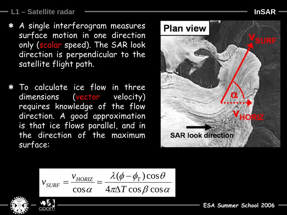
A single interferogram measures surface motion in one direction only (scalar speed). The SAR look direction is perpendicular to the satellite flight path.
To calculate ice flow in three dimensions (vector velocity) requires knowledge of the flow direction. A good approximation is that ice flows parallel, and in the direction of the maximum surface:
αβπθφφλ
α coscos4cos)(
cos Tvv THORIZ
SURF Δ−
==
InSAR
ESA Summer School 2006
L1 – Satellite radar
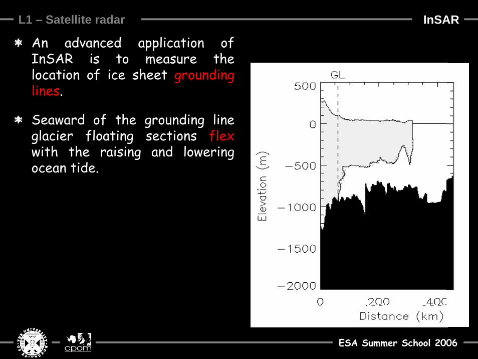
An advanced application of InSAR is to measure the location of ice sheet grounding lines.
Seaward of the grounding line glacier floating sections flexwith the raising and lowering ocean tide.
InSAR

ESA Summer School 2006
L1 – Satellite radar
Differencing fourinterferograms eliminates ice motion and fixed topography to reveal tidal motion.
The tidal flexure hinge line(close to the grounding line) is clearly visible in quadruple-difference interferograms.
The major application of this technique is to monitor migrationof glacier grounding lines over time, to determine their retreat or advance.
InSAR

ESA Summer School 2006
L1 – Satellite radar InSAR
Rignot et al (2002) computed the mass budget of 60% of the Antarctic ice sheet using InSAR.
They calculated the ice sheet was losing 26 ± 37 Gt yr-1.

ESA Summer School 2006
L1 – Satellite radar Summary
Estimates of Antarctic mass balance

ESA Summer School 2006
L1 – Satellite radar Summary
Estimates of Antarctic mass balance
Glaciology
Mass budget
Volume change
Method
-40 ± 480Various
-26 ± 37
-60 ± 76
Mass Balance(Gt)
Rignot, 2002
Wingham, 1998
Study
Satellite RADAR has brought about a factor 10 improvement in theprecision of the Antarctic ice sheet sea level contribution