L section towers

8/13/2019 L section towers

http://slidepdf.com/reader/full/l-section-towers 1/15

A general three-dimensional L-section beam nite elementfor elastoplastic large deformation analysis

Phill-Seung Lee *, Ghyslaine McClureCivil Engineering and Applied Mechanics, McGill University, Montreal, Quebec, Canada H3A 2K6

Received 22 April 2005; accepted 16 September 2005Available online 15 November 2005

Abstract

In this paper, the development of a general three-dimensional L-section beam nite element for elastoplastic large deformation anal-ysis is presented. We propose the generalized interpolation scheme for the isoparametric formulation of three-dimensional beam niteelements and the numerical procedure is developed for elastoplastic large deformation analysis. The formulation is general and effectivefor other thin-walled section beam nite elements. To show the validity of the formulation proposed, a 2-node three-dimensional L-sec-tion beam nite element is implemented in an analysis code. As numerical examples, we rst perform elastic small and large deformationanalyses of a cantilever beam structure subjected to various tip loadings, and elastoplastic large deformation analysis of the same struc-ture under reversed cyclic tip loading. We then analyze the failures of simply supported beam structures of different lengths and slender-ness ratios under elastoplastic large deformation. The same problems are solved using rened shell nite element models of the structures.The numerical results of the L-section beam nite element developed here are compared with the solutions obtained using shell niteelement analyses. We also discuss the numerical solutions in detail.

2005 Elsevier Ltd. All rights reserved.

Keywords: Beam structures; L-section beams; Finite elements; Nonlinear analysis; Elastoplastic material; Large deformation

1. Introduction

Thin-walled section beams including L-section (angle)shapes have been widely used in metallic frameworks forbuildings, industrial structures and lattice structures. Non-linear analysis considering large deformations and inelasticmaterial is very important for investigating the load-bear-ing capacity of beam structures. In practice, the nite ele-

ment method is the main tool for such analyses of beamstructures [1]. The behavior of thin-walled beams (in partic-ular, non-symmetric thin-walled sections) while undergoinginelastic large deformations is very complex and hard topredict using beam nite elements. In fact, the full three-dimensional nonlinear behavior of such sections can berepresented more accurately using shell nite elements.However, for structures with a large number of thin-walled

beam members, such as lattice structures, this approach isnot practical because of the large modeling effort and com-putational time required.

Considerable effort has been put on the development of symmetric and non-symmetric section beam nite elementsfor elastic large deformation analysis and valuable resultshave been obtained, see Refs. [2–4] and therein. However,considering inelastic material, it is very hard to formulate

such beam nite elements and only successes for relativelysimple symmetric cross-sections (rectangular solid, I-shape,square and circular hollow sections [5–7]) have beenreported. The development of general (symmetric or non-symmetric) section beam nite elements for inelastic largedeformation analysis, which are simple and effective, is stillopen and the challenge is continuing.

In this paper, we propose a generalized interpolationscheme for the isoparametric formulation of three-dimen-sional beam nite elements, which can be used for both sym-metric and non-symmetric section beams. The formulation

0045-7949/$ - see front matter 2005 Elsevier Ltd. All rights reserved.doi:10.1016/j.compstruc.2005.09.013

* Corresponding author. Tel.: +1 514 573 3477; fax: +1 514 398 7361.E-mail address: [email protected] (P.S. Lee).

www.elsevier.com/locate/compstrucComputers and Structures 84 (2006) 215–229

mailto:[email protected]

mailto:[email protected]



and numerical procedure are developed for elastoplasticlarge deformation analysis of L-section beams. Note thatthe formulation is simple and effective for general (thin-walled) section beam nite elements. Since, in researcharticles, we could not nd analysis examples or studies onthree-dimensional L-section beam nite elements for elasto-

plastic large deformation analysis, we show the validity of the element proposed using the solution of shell nite ele-ment models.

The isoparametric approach has been widely used forthe general curved beam nite element [1], because trans-verse shear strain is automatically considered and theformulation is general and effective, in particular, for non-linear analysis. When the dimensions of the beam sectionare small compared to the beam length, the displacement-based isoparametric beam nite element locks, that is,the element is too stiff in bending problems. In spite of this disadvantage, this type of beam nite element isvery attractive because the formulation is directly derivedfrom three-dimensional continuum mechanics and easilyextended to nonlinear analysis. Locking can be removedusing reduced-order integration or a mixed formulation [1].

In this study, our main objective is to develop a generalthree-dimensional L-section beam nite element, which isgeneral and reliable for elastoplastic large deformationanalysis as well as linear elastic analysis. For effective non-linear analysis of three-dimensional frameworks usingbeam nite elements, the following are necessary:

• Full three-dimensional behavior,• Consideration of axial, bending and shearing actions,• Availability for short and long beams (various slender-ness ratios),• Geometrical nonlinear capability (for large deformation

and buckling behavior),• Material nonlinear capability (in particular, for elasto-

plastic material),• Consideration of loading and displacement

eccentricities.

In the following sections, we present the isoparametricformulation of a general three-dimensional L-section beamnite element for elastoplastic large deformation analysisand show the numerical performance of the formulation.We propose the generalized geometry and displacementinterpolation scheme for the isoparametric beam nite ele-ments, which can automatically consider the eccentricitiesof loading and boundary conditions. To illustrate theapplication of this formulation and discuss its perfor-mance, we implement a 2-node L-section beam nite ele-ment in an analysis code. As numerical tests, we performelastic small and large deformation analyses of an L-sec-tion cantilever beam structure subjected to various staticloadings, and the elastoplastic large deformation analysisof the same structure under reversed cyclic tip loading.The failures of simply supported beam structures (of differ-ent length) under elastoplastic large deformation are ana-

lyzed. The results are compared with the solutionsobtained with rened shell nite element models of thestructures.

2. L-section beam nite element

In this section, we present the nonlinear formulation of the general three-dimensional L-section isoparametricbeam nite element for elastoplastic large deformationanalysis.

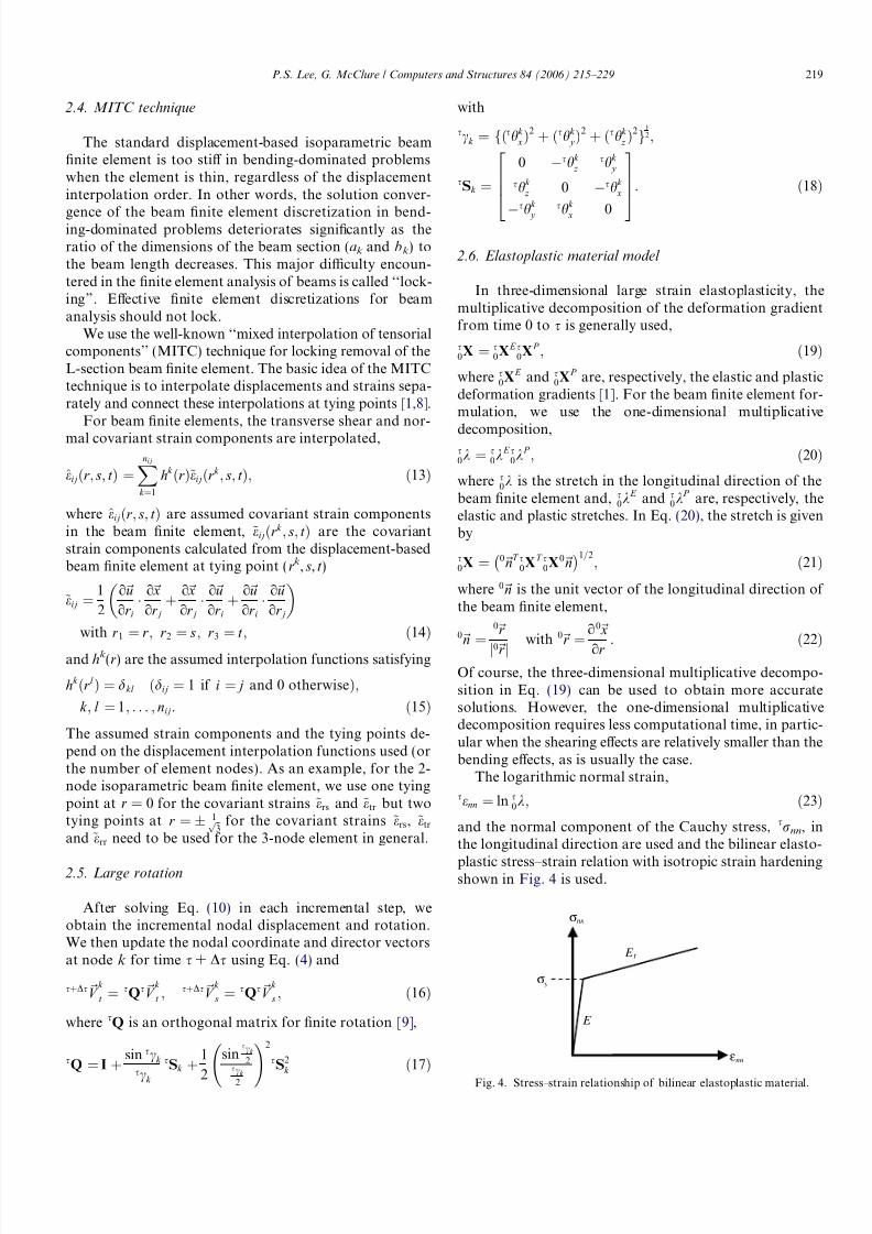
We rst propose generalized geometry and displacementinterpolations that can be used for beam nite elements of all possible section shapes, and we present the example of the L-section shape beam here. Considering large deforma-tion and elastoplastic behavior, the updated Lagrangianformulation is adopted. We also use the ‘‘mixed interpola-tion of tensorial components’’ (MITC) technique for thelocking removal [1,8]. To consider large rotation kinemat-ics, the director vectors of the beam nite element areupdated after each time increment using an orthogonalmatrix for nite rotations as described in [9]. For elasto-plastic analysis, we use the logarithmic strain calculatedfrom the one-dimensional multiplicative decomposition of the longitudinal stretch of the beam [1].

In this paper, we use the superscript or subscript s todenote time, but, in static analysis, s is a dummy variableindicating load levels and incremental variables rather thanactual time as in dynamic analysis [1].

2.1. Geometry and displacement interpolations

The basic kinematic assumption of the beam formula-tion is that plane cross-sections originally perpendicularto the central axis of the beam remain plane and undis-torted under deformation but not necessarily perpendicularto the central axis of the deformed beam. In order to intro-duce a more general isoparametric beam formulation,instead of using the central axis, we use a longitudinalreference line, which does not need to pass through thecentroid of the beam section. This reference line can bearbitrarily positioned on the beam section depending onthe location of the nodal degrees of freedom; this featureautomatically facilitates consideration of loading and dis-placement eccentricities at the nite element level.

Considering the longitudinal reference line in Fig. 1, thegeometry of the q-node beam nite element at time s isinterpolated by

s~ xðr ; s; t Þ ¼Xq

k ¼1hk ðr Þs~ xk þX

q

k ¼1

t t k

2 ak hk ðr Þs ~V

k t

þXq

k ¼1

s sk

2 bk hk ðr Þs ~V

k s ; ð1Þ

where hk (r) are the interpolation polynomials in usual iso-parametric procedures, s~ xk are the Cartesian coordinates of node k at time s, ak and bk are the cross-sectional dimen-

sions (length of legs in L-section shapes) at node k , and

216 P.S. Lee, G. McClure / Computers and Structures 84 (2006) 215–229



the unit vectors s~V k t and s~V

k s are the director vectors in

directions t and s at node k and at time s. Note that s~V k t

and s~V k s are normal to each other, and these vectors are

parallel to the two legs of the L-section, as shown in Fig. 1.In Eq. (1), the variables sk and t k are used to position the

nodal degree of freedom (or the reference longitudinal line)in the beam nite element. In effect, these variables shift the

domain in the natural coordinate system ( s, t) as follows:1 6 s 6 11 6 t 6 1 ) 1 sk 6 s sk 6 1 sk ;

1 t k 6 t t k 6 1 t k . ð2ÞAs illustrated in Fig. 2, sk and t k are calculated from thelocation of the nodal degree of freedom and the cross-sec-tional dimensions. Let us consider the nodal Cartesiancoordinate system dened by the director vectors s~V

k

t ands ~V

k s at node k . The points c and c0 are the position of the

nodal degree of freedom and the center of the dotted rect-

angle, respectively. Due to the geometrical proportionalitybetween Fig. 2(a) and (b), we obtain

sk ¼ 2 xk

bk ; t k ¼ 2

y k

a k ; ð3Þ

where xk and y k represent the projected distances between cand c0 in the nodal Cartesian coordinate system at node k .This shifting of the domain in the natural coordinate sys-tem allows a general description of the geometry interpola-tion. Consequently, the positions of the nodal degrees of freedom can be arbitrarily located on the beam sections.

The Cartesian coordinate of a point at time s + D s issþD s~ x ¼ s~ x þ s~u; ð4Þwhere s~u is the incremental displacement from time s tos + D s .

Substituting Eq. (1) into Eq. (4) and using the second-order approximations for the large rotation of the directorvectors, we obtain the incremental displacement from times to s + D ss~u

¼ s~ua

þ s~ub

ð5

Þwith

s~ua

ðr ; s; t Þ ¼Xq

k ¼1hk ðr Þs~uk þX

q

k ¼1

t t k

2 ak hk ðr Þ s~hk s ~V

k t h i

þXq

k ¼1

s sk

2 bk hk ðr Þ½s~hk s ~V

k s ;

s~ub

ðr ; s; t Þ ¼Xq

k ¼1

t t k

4 ak hk ðr Þ s~hk ðs~hk s ~V

k t Þh i

þXq

k ¼1

s sk

4 bk hk ðr Þ½s~hk ðs~hk s ~V

k sÞ;

ð6Þ

(b)(a)

sc

'c

c

'c

t

k b

k a

k s

k t k y

k d

k e

k x

0.2

0.2

k

k

bd

2

k

k

ae

2

k

t V

k sV

→

→

τ

τ

Fig. 2. Geometric description of xk , y k , sk and t k at node k : (a) in the nodalCartesian coordinate system and (b) in the natural coordinate system.

y

v y,

yi

zi

x i u x , x

z, w

z

k d

k a

k b

r s

t

k e

k– 1a

k– 1b

Longitudinalreference line

Node k

Node k-1k t V

k sV

k– 1sV

k– 1t V

θ

θ

θ

→

→

→

→

→

→

→τ

τ

ττ

Fig. 1. Geometry of a general three-dimensional L-section beam element.

P.S. Lee, G. McClure / Computers and Structures 84 (2006) 215–229 217



in which the incremental rotation vector at node k is

s~hk ¼s hk

xs hk

y

s hk z

264375

; ð7Þ

and the displacement s

~ub

is the additional term derivedfrom the second-order approximations for the large rota-tion of the director vectors. Of course, this term is not nec-essary for linear analysis. This additional displacement is aquadratic expression in rotations and is used for the non-linear formulation of the beam nite element.

2.2. Finite element discretization

Using the principle of virtual displacement at times + D s , the linearized equilibrium equation in the updatedLagrangian formulation is obtained for the beam niteelement,

Z s V sC ijkm sea

kmdseaij dsV þZ s V

ss ijðdsgaij þ dseb

ijÞdsV

¼ sþD s R Z s V

s r ij dseaij dsV ; ð8Þ

where s V , s C ijkm and s r ij are the volume, the material lawand the Cauchy stress tensor at time s, respectively, ands ea

km ¼ 12 ðsua

k ;m þ s uam;k Þ are the linear terms of the strain ten-

sor corresponding to the displacement s~ua at time s,ds ea

ij ¼ 12 ðdsua

i; j þ dsua j ;iÞ are the linear terms of the strain ten-

sor corresponding to the virtual displacement ds~ua at times , dsga

ij

¼ 12

ðds ua

k ;isua

k ; j

þ s ua

k ;idsua

k ; j

Þ are the nonlinear terms

of the strain tensor corresponding to the virtual displace-ment ds~ua at time s, and dseb

ij ¼ 12 ðds ub

i; j þ dsub j ;iÞ are the

components of the strain tensor corresponding to the vir-tual displacement ds~ub at time s.

The term sþD s R in the right-hand side of Eq. (8) repre-sents the externally applied forces,

sþD s R ¼Z sþD s V

sþD s f Bi dui dsþD s V þZ sþD s S f

sþD s f S i duS

i dsþD sS ;

ð9Þwhere sþD s f Bi are the components of the externally appliedforce per unit volume at time s + D s , sþD s f S

i are the compo-nents of the externally applied surface traction per unitsurface area at time s + D s , s + D s S f is the surface at times + D s on which external tractions are applied, and duS

iare dui evaluated on the surface s + D s S f .

Substituting Eqs. (1) and (6) into (8), we obtain thematrix form of the linearized equilibrium equation in theupdated Lagrangian formulation [1],s KsU ¼ sþD s R s F ; ð10Þwhere s K is the tangent stiffness matrix at time s , s U is theincremental nodal displacement vector, s + D s R is the vectorof externally applied nodal load at time s + D s , and s F isthe vector of nodal forces equivalent to the element stresses

at time s . s K consists of both the geometric linear and non-linear stiffness matrices (s K = s KL + s KNL ).

2.3. Numerical integration

In order to obtain the tangent stiffness matrix and vec-

tors of Eq. (10), we perform the numerical integration overthe two legs of the L-section, which are placed in the r tand r s planes (see Figs. 1–3),

Z V A dV ¼Z

1

1 Z 1

1½grt A det J s¼ 1 dt dr

þZ 1

1 Z 1

1½grsA det J t ¼ 1 d sdr ; ð11Þwhere A is a generic matrix or vector function, det J is thedeterminant of the three-dimensional Jacobian matrix andthe factors grt and g rs are

grt ¼ 2Xq

k ¼1hk ðr Þd k

Xq

k ¼1hk ðr Þbk

, ;

grs ¼ 2Xq

k ¼1hk ðr Þek X

q

k ¼1hk ðr Þa k , ð12Þ

Gaussian quadrature is used for the integration in Eq. (11).For example, Fig. 3 shows the eight integration points forthe elastic analysis of the 2-node L-section beam nite ele-ment and the coordinates of the integration points aregiven in Table 1 . Of course, more integration points inthe s and t directions are required for inelastic analysisand the solution accuracy depends on the number of inte-

gration points. This is further discussed in Section 3.

Fig. 3. Gauss integration points of the 2-node L-section beam element inthe natural coordinate system.

Table 1Integration points in the natural coordinate system for elastic analysis

r – t plane r – s plane

i r s t i r s t

1 1= ffiffiffi3p 1 1= ffiffiffi3p 5 1= ffiffiffi3p 1= ffiffiffi3p 12 1= ffiffiffi3p 1 1= ffiffiffi3p 6 1= ffiffiffi3p 1= ffiffiffi3p 13 1=

ffiffiffi3p 1 1=

ffiffiffi3p 7 1=

ffiffiffi3p 1=

ffiffiffi3p 1

4 1= ffiffiffi3p 1 1= ffiffiffi3p 8 1= ffiffiffi3p 1= ffiffiffi3p 1




3. Numerical tests

To investigate in detail the predictive capability of the proposed numerical scheme, we implement the 2-nodeL-section beam nite element in an analysis code and per-form numerical studies for various beam problems. In this

section, we report upon the various numerical results of theL-section beam nite element proposed in this study.Let us consider the beam structure shown in Fig. 5. The

beam is straight and has an L-shape section with two legs

of lengths, W and H . The legs have a constant thickness,h, and are normal to each other. The section prole is con-stant along the beam axis. The beam is then given variousboundary conditions and loadings at ends A and B , whichallows to simulate various structural behaviors. In the fol-lowing section, we perform the elastic small and large

deformation, elastoplastic large deformation and elasto-plastic failure analyses using the 2-node beam nite ele-ments developed.

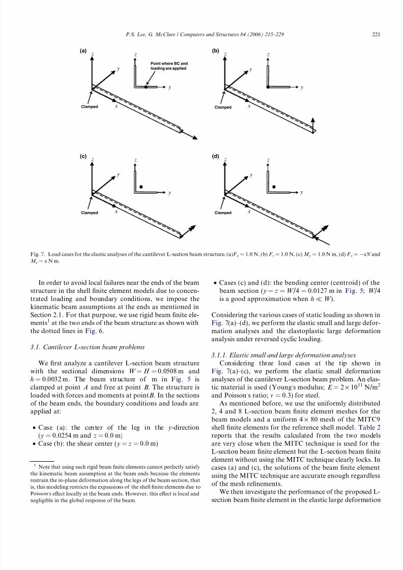
The results obtained with the beam nite elements arecompared with the rened solutions of the MITC9 shellnite elements in ADINA [10]. The reliable performanceof the MITC9 shell nite element has been demonstratedin the literature [11,12]. For the shell nite element models,a uniform mesh is used in each leg and along the axialdirection and for the beam nite element models, a uniformmesh of 2-node beam elements is used along the axial direc-tion. Fig. 6 shows the meshes used for the shell (2 · 20 ele-ments) and beam (eight elements) nite element models.After studying the solution convergence of the shell niteelement models, we selected the mesh of the shell nite ele-ment models which can be used as reference.

In this study, we use only uniform meshes, which is notoptimal for efficient numerical solution in general. How-ever, since uniform meshes are frequently used in practice,it is valuable to use them to investigate the numerical per-formance of the proposed beam nite element.

z

x

y

A

B

z

y

L

H

W

h

h

Fig. 5. L-section beam structure.

y

zRigid beam elementsat ends only

Point where BC andloading are applied

Beam model(8 beam elements)

Shell model (2x20MITC9 elements)

Fig. 6. Beam and shell nite element models of the L-section beam structure.




Table 2Tip displacements calculated in the linear elastic analyses of the cantilever L-section beam structure using the MITC technique

Mesh Case (a) Case (b) Case (c)

dx d y, dz d y dz d y dz

Beam (1el.) 1.07653e 7 3.63282e 6 8.58098e 4 1.43045e 3 4.29073e 4 7.15122e 4Beam (2el.) 1.07653e 7 3.63282e 6 1.07264e 3 1.78801e 3 4.29073e 4 7.15122e 4

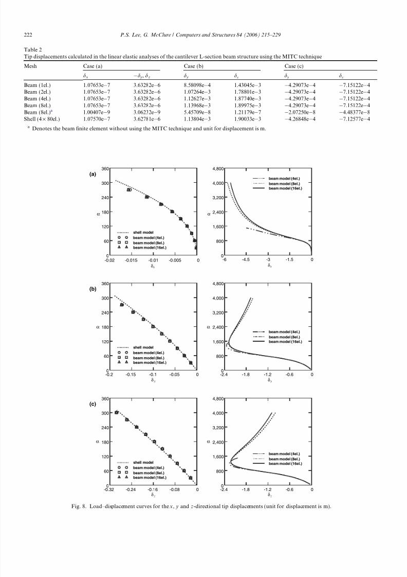
Beam (4el.) 1.07653e 7 3.63282e 6 1.12627e 3 1.87740e 3 4.29073e 4 7.15122e 4Beam (8el.) 1.07653e 7 3.63282e 6 1.13968e 3 1.89975e 3 4.29073e 4 7.15122e 4Beam (8el.)a 1.00407e 9 3.06232e 9 5.45709e 8 1.21179e 7 2.07250e 8 4.48377e 8Shell (4 · 80el.) 1.07570e 7 3.62781e 6 1.13804e 3 1.90033e 3 4.26848e 4 7.12577e 4

a Denotes the beam nite element without using the MITC technique and unit for displacement is m.

shell modelbeam model (4el.)beam model (8el.)beam model (16el.)

-0.02 -0.015 -0.01 -0.005 00

60

120

180

240

300

360

x

(a)

-0.2 -0.15 -0.1 -0.05 00

60

120

180

240

300

360


(b)

-0.32 -0.24 -0.16 -0.08 00

60

120

180

240

300

360


(c)

-6 -4.5 -3 -1.5 00

800

1,600

2,400

3,200

4,000

4,800

-2.4 -1.8 -1.2 -0.6 00

800

1,600

2,400

3,200

4,000

4,800

-2.4 -1.8 -1.2 -0.6 00

800

1,600

2,400

3,200

4,000

4,800

beam model (4el.)beam model (8el.)beam model (16el.)



δ x δ

yδ yδ

zδ zδ

α α

α α

α α

Fig. 8. Load–displacement curves for the x , y and z-directional tip displacements (unit for displacement is m).




analysis. The cantilever L-section beam is subjected to thetip loading shown in Fig. 7(d) and the elastic large defor-mation analysis is performed using the same elastic mate-rial (steel) as in the elastic small deformation analyses.The loading factor a is increased statically and the tip dis-placements in the x, y and z directions are measured. We

calculate the solutions using the uniform 4 · 80 mesh of the shell model and the uniform 4, 8 and 16 element meshesof the beam model.

Fig. 8 shows the load–displacement ( a – d) curves in thetwo ranges of loading (up to a = 300 and a = 4000). Thesolutions of the shell nite element model are not obtainedfor the loading factor larger than a = 300 due to local fail-ure in the numerical solution. When 4, 8 and 16 L-sectionbeam nite elements are used in the beam model up toa = 300, the responses of the L-section beam nite elementsagree with those of the shell nite element model. Theload–displacement curves up to a = 4000 show that the

solution of the beam model using 4 L-section beam niteelements lacks accuracy compared to the solutionsobtained with 8 and 16 L-section beam nite elements in

-2 -1 0 1 2 3 4

-2.4

-2

-1.6

-1.2

-0.8

-0.4

0

0.4

α = 500

α = 0

α = 1000

α = 4000

x

z y,

x-y plane

x-z plane

Fig. 9. Deformed shapes projected in the x – y and x – z planes for a mesh of 16 elements (unit is m).

N –200

Time

N 200

2x2 points 2x4 points 2x7 points

Reversed cyclic loading

z

x

y

Clamped

α

Fig. 10. Static reversed cyclic loading (F y = F z = aN ) and numerical integration points used in the beam section.

-0.5 -0.4 -0.3 -0.2 -0.1 0 0.1-240

-160

-80

0

80

160

240

-0. 8 -0.4 0 0.4 0.8 1.2 1.6

-240

-160

-80

0

80

160

240

x

(a)

(b)

shell modelbeam model (2x2pt.)beam model (2x4pt.)beam model (2x7pt.)

shell modelbeam model (2x2pt.)beam model (2x4pt.)beam model (2x7pt.)

δ

yδ

α

α

Fig. 11. Load–displacement curves for the (a) x- and (b) y-directional tipdisplacements (unit for displacement is m).




the very large deformation range. Fig. 9 displays thedeformed shapes of the cantilever projected in the x – yand x – z planes at various load levels for the case with amesh of 16 beam nite elements.

3.1.2. Elastoplastic large deformation analysis

We perform here the elastoplastic large deformationanalysis under a reversed cyclic loading using the beamand shell nite element models described in the previoussection. The properties of the bilinear elastoplastic material(see Fig. 4) used are:

• Young s modulus: E = 2 · 1011 N/m 2,• Yield stress: r y = 250 · 106 N/m 2,• Poisson s ratio: m = 0.3,• Strain hardening modulus: E t = 2.0 · 1010 N/m 2.

z

x

y

A

B L

m0508.0

m0508.0

m.00320

m0032.0

z

y

m015.0

x δ

Fig. 12. A simply supported L-section beam with a section of equal legs.

Fig. 13. Non-scaled deformed shapes and accumulated effective plastic strain distributions. (a) L = 0.25 m, dx = 0.0004 m (2 · 5el. mesh), (b) L = 1.0 m,dx = 0.008 m (4 · 20 el. mesh), (c) L = 4.0 m, dx = 0.06 m (4 · 80 el. mesh).




As shown in Fig. 10, a reversed cyclic loading is stati-cally applied at the shear center of the free end of the beam( y = z = 0.0 m in Fig. 5). We use the uniform 4 · 80 meshfor the reference shell model and the uniform 8 element

mesh of L-section beam nite elements for the beam niteelement model. Varying the number of numerical integra-tion points as shown in Fig. 10, the solutions arecalculated.

0 0.002 0.004 0.006 0.0080

8,000

16,000

24,000

32,000

40,000

48,000

shell model (4x20el.)

beam model (16el.)beam model (8el.)


plastic hinge

D

E

R

0 0.0001 0.0002 0.0003 0.00040

15,000

30,000

45,000

60,000

75,000

90,000




yielding

D

x

R

(b)

(a)

equation (24)

0 0.015 0.03 0.045 0.060

1,000

2,000

3,000

4,000

5,000




plastic hinge

elasticbuckling

ED

F R

(c)

equation (24)

δ

x δ

x δ

Fig. 14. Reaction–displacement curves for (a) L = 0.25 m and (b) L = 1.0 m and (c) L = 4.0 m. (Unit for reaction is N and unit for displacement is m.)




Fig. 11(a) and (b) display the load–displacement curvesfor the x - and y-directional tip displacements, respectively.Due to the symmetry of the problem, the z-directional dis-placement is equal to the y-directional displacement. Afterone cycle of loading, the residual displacements due to plas-tic strain are observed. As the number of integration points

increases, the solutions of the beam nite element modelconverge toward the reference shell nite element solutions.When the 7-point numerical integration scheme is used ineach leg of the beam section, the responses calculated usingthe L-section beam nite elements show very good agree-ment with the reference solutions obtained with the MITC9shell nite element model. The 7-point numerical integra-tion is therefore recommended for inelastic analysis usingthe L-section beam nite element proposed in this paper.

3.2. Elastoplastic failure analyses of a simplysupported beam

Let us consider a simply supported straight L-sectionbeam structure of length L , shown in Fig. 12. The structurehas equal legs (W = H = 0.0508 m) of uniform thicknessh = 0.0032 m. Three different beam lengths of 0.25 m, 1 mand 4 m are considered. The structure is subjected to a pre-scribed axial displacement dx at point B in the x directionand the boundary conditions imposed are: ux = u y = uz =hx = 0 at point A and u y = uz = 0 at point B .

It should be noted that points A and B in Fig. 12 areeccentric with respect to the centroid (bending center) of the beam section. This eccentricity can be considered asan initial imperfection of the beam structures and can

induce instability (or buckling) when the beam structureis slender enough. The position of the centroid in the y z plane is y = z = 0.0127 m in Fig. 12 and points Aand B are at y = z = 0.015 m. Therefore, the eccentricityis e y = ez = 0.0023 m in the y and z directions.

We use a bilinear elastoplastic material model,

• Young s modulus: E = 2 · 1011 N/m 2,• Yield stress: r y = 250 · 106 N/m 2,• Poisson s ratio: m = 0.3,• Strain hardening modulus: E t = 0.1 N/m 2.

Using the MITC9 shell nite elements, the three prob-lems (corresponding to L = 0.25 m, 1 m and 4 m) describedabove are analyzed. Fig. 13 displays the non-scaleddeformed shapes and accumulated effective plastic straindistributions of the simply supported L-section beam struc-tures modeled using the MITC9 shell nite elements. InFig. 13(b) and (c), plastic hinges are observed at mid lengthof the beam structures.

In the analysis using the L-section beam nite element,the 7-point per leg numerical integration is adopted asrecommended in Section 3.1.2 and we use the 4, 8 and 16uniform element meshes in the longitudinal direction.

Fig. 14(a) shows the reaction–displacement curves at thetip (point B in Fig. 12), when the beam length is 0.25 m.

The axial reaction is measured at the same point wherethe displacement is prescribed. The curves represent typicallinear elastic behavior up to point D in Fig. 14(a). Afterthat point, yielding of the longitudinal bers of the beamunder compression occurs, which clearly governs the fail-ure of this short beam. The results of the 2-node L-section

beam nite element developed show almost the same curvesas the solutions calculated from the shell nite elementmodels.

The reaction–displacement curves of the 1.0 m beam areshown in Fig. 14(b). The behavior of this beam is morecomplex than the 0.25 m beam. Up to point D in thecurves, the behavior is linear elastic. The beam then startsyielding and excessive bending develops at mid length of the beam where a plastic hinge suddenly occurs at pointD . The plastic hinge and the P D effect rapidly reducethe load-bearing capacity of the beam structure. The failuremode is dominated by plastic hinging and then the P Deffect.

The decreasing load-bearing capacity of this case can beexplained by a simple model. When a simply supportedbeam with a plastic hinge buckles under a compressive loadP , the plastic post-buckling response is approximatelygiven by

P ¼ 2 M p

ffiffiffiffiffiffiffiffiffi L2 ð L dÞ2q

; ð24Þ

where M p is the plastic moment of the beam section, L isthe length of the beam and d is the axial displacement. Thisequation can be easily derived from the model in Fig. 15.We also plot the curve given by Eq. (24) in Fig. 14(b).

It is interesting to note that, in our numerical solution,there is a sudden change in the response curves of the shellnite element model (4 · 20 mesh) at point E but not in thebeam nite element solutions. This behavior results fromthe local failure at the center of the beam structure dueto the excessive deformation. Fig. 16 shows the deformedshape and accumulated effective plastic strain distributionsbefore and after point E . A similar phenomenon happensin the numerical solution of the 2 · 20 mesh shell modelbut the position of the dropping point is different.

p M

P

2 L

(2

1 L – δ )

22 )(2

1 L – δ L –

Plastic hinge

δ

Fig. 15. Buckling of a simply supported beam with a plastic hinge at midlength.




The theoretical elastic buckling load of this beam is

P cr ¼ p2 EI min

L2 69; 000N; ð25Þwhere I min is the minimum second moment of area of thebeam section. However, the beam starts its failure whenthe reaction is about 60% of the buckling load because of the plastic hinge effect.

All the curves in Fig. 14(b) obtained from the beam andshell nite element models show a very similar response inthe elastic range. However, after the plastic hinge occurs atthe center of the beam structure, the beam nite elementsolutions show some difference with the results of the shellnite element models because of the local failure observedat mid length in the numerical solution of the shell models.

Fig. 14(c) shows the numerical results when the length of the beam structure is 4 m. Buckling of the beam structurestarts at point D and the plastic hinge occurs at point E .The failure of this slender beam structure is clearly dueto elastic buckling. The theoretical elastic buckling loadcalculated is P cr

4300 N, which matches well with point

D in the response curves. For the same reason as explained

in the case of the 1.0 m beam structure, the solutions of theL-section beam nite element show different responses afterdropping point F obtained with the shell nite elementsolution. It is also noted that Eq. (24) shows good agree-ment with the beam numerical solutions.

We report that, considering computational timerequired for comparable accuracy, the beam nite elementmodel is about 2.5 times 2 efficient than the shell nite ele-

ment model when the beam length is equal to 4 m. How-ever, as the beam length decreases, the computationaladvantage of the beam nite element model becomessmaller.

As a last numerical example, we modeled the threesimple beam problems with a section of unequal legs asshown in Fig. 17. The same prescribed axial displacementsas in the previous example are applied at the shear centerof the beam sections, that is, there is eccentricity. Thesame material properties are used and the 7-point per leg

Fig. 16. Local failure at the mid length (a) before point E (b) after point E shown in Fig. 14(b).

2 This ratio is obtained using the same solver in our analysis code for thebeam and shell nite element models. Note that, in general, the ratiodepends on a solver used to calculate the numerical solution.




numerical integration is used for the beam nite elementmodels. Fig. 18 shows the reaction–displacement curvesin each case and the non-scaled deformed shape when thebeam length L is equal to 1 m. It is observed that the reac-tion–displacement curves of the beam and shell nite ele-ment models show good agreement when eight beamnite elements are used.

Finally, we discuss when it is better to use the beam orshell nite element models. Considering the modeling effortand the computational time required to obtain an accuratesolution, we nd that for a simple structure with few L-sec-tion beam members, the beam nite element model is notmuch better than the shell nite element model. However,for structures with a large number of the L-section beam

0 0.0003 0.0006 0.0009 0.00120

8,000

16,000

24,000

32,000

40,000

48,000

0 0.004 0.008 0.012 0.0160

5,000

10,000

15,000

20,000

25,000

30,000

0 0.02 0.04 0.06 0.080

1,500

3,000

4,500

6,000

7,500

x

(a) (b)

(c)

R

R

R

original configuration

deformed shape

(d)

beam model (2el.)shell model (4x80el.)






δ

x δ

x δ

Fig. 18. Reaction–displacement curves for (a) L = 0.25 m, (b) L = 1.0 m and (c) L = 4.0 m, and (d) non-scaled deformed shape for L = 1.0 m anddx = 0.01 m. (Unit for reaction is N and unit for displacement is m.)

z

x

y

A

L

m.0640

m.05080

m.00320

m.00320

z

y

Shear center

x

B

δ

Fig. 17. A simply supported L-section beam with a section of unequal legs.




members and for predicting the global responses, the beamnite element model is obviously much more efficient.

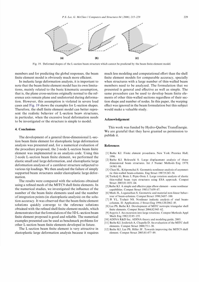
In inelastic large deformation analysis, it is important tonote that the beam nite element model has its own limita-tions, mainly related to the basic kinematic assumption,that is, the plane cross-sections originally normal to the ref-

erence axis remain plane and undistorted during deforma-tion. However, this assumption is violated in severe loadcases and Fig. 19 shows the examples for L-section shapes.Therefore, the shell nite element model can better repre-sent the realistic behavior of L-section beam structures,in particular, when the excessive local deformation needsto be investigated or the structure is simple to model.

4. Conclusions

The development of a general three-dimensional L-sec-tion beam nite element for elastoplastic large deformationanalysis was presented and, for a numerical evaluation of the procedure proposed, the 2-node L-section beam niteelement was implemented in an analysis code. Using this2-node L-section beam nite element, we performed theelastic small and large deformation, and elastoplastic largedeformation analyses of a cantilever structure subjected tovarious tip loadings. We then analyzed the failure of simplysupported beam structures under elastoplastic large defor-mation.

The results were compared with the solutions obtainedusing a rened mesh of the MITC9 shell nite elements. Inthe numerical studies, we investigated the inuence of thenumber of the beam nite elements used and the number

of integration points (in elastoplastic analysis) on the solu-tion accuracy. It was observed that the beam nite elementsolutions quickly converge to the reference solutionsobtained with the rened shell nite element models, whichdemonstrates that the formulationof the 3D L-section beamnite element proposed is good and reliable. The numericalexamples presented can be used as benchmark problems forother L-section beam nite elements developed in future.

The L-section beam nite element is very attractive inelastoplastic large deformation analysis because it requires

much less modeling and computational effort than the shellnite element models for comparable accuracy, speciallywhen structures with a large number of thin-walled beammembers need to be analyzed. The formulation that wepresented is general and effective as well as simple. Thesame procedure can be used to develop beam nite ele-

ments of other thin-walled sections regardless of their sec-tion shape and number of nodes. In this paper, the warpingeffect was ignored in the beam formulation but this subjectwould make a valuable study.

Acknowledgement

This work was funded by Hydro-Que ´bec TransE nergie.We are grateful that they have granted us permission topublish it.

References

[1] Bathe KJ. Finite element procedures. New York: Prentice Hall;1996.

[2] Bathe KJ, Bolourchi S. Large displacement analysis of three-dimensional beam structures. Int J Numer Methods Eng 1979;14:961–86.

[3] Chan SL, Kitipornchai S. Geometric nonlinear analysis of asymmet-ric thin-walled beam-columns. Eng Struct 1987;9:243–54.

[4] Turkalj G, Brnic J, Prpic-Orsic J. Large rotation analysis of elasticthin-walled beam type structures using ESA approach. ComputStruct 2003;81:1851–64.

[5] Bathe KJ. A simple and effective pipe elbow element—some nonlinearcapabilities. Comput Struct 1983;17:659–67.

[6] Meek JL, Loganathan S. Geometric and material non-linear behav-iour of beam-columns. Comput Struct 1990;34:87–100.

[7] Pi YL, Trahair NS. Nonlinear inelastic analysis of steel beam-columns. II: Applications. J Struct Eng 1994;120:2062–85.

[8] Lee PS, Bathe KJ. Development of MITC isotropic triangular shellnite elements. Comput Struct 2004;82:945–62.

[9] Argyris J. An excursion into large rotations. Comput Methods ApplMech Eng 1982;32:85–155.

[10] ADINA R&D Inc. ADINA theory and modeling guide, 2003.[11] Bathe KJ, Iosilevich A, Chapelle D. An evaluation of the MITC shell

elements. Comput Struct 2000;75:1–30.[12] Bathe KJ, Lee PS, Hiller JF. Towards improving the MITC9 shell

element. Comput Struct 2003;81:477–89.

Fig. 19. Deformed shapes of the L-section beam structure which cannot be predicted by the beam nite element model.


L section towers

Documents

Transcript of L section towers