L 0CL R A EPOR T TE CH N IC AL R E POR T · r----- ---- nI II I I I I I I Sand*.., L 0CL R A EPOR T...

r--------------------- ---- nI

III II II I

Sand*.., L 0CL R A EPOR TII TE CH N IC AL R E POR T

NO. 12685 III

Propagation of Visible and InfraredRadiation by Fog, Rain, and Snow

Contract No. DAAE07-81-G-4006

July, 1982

L. W. Winchester, Jr.and

by G. G. Gimmestad

S~Keweenaw Research CenterMichigan Technological University

! Houghton, Michigan 49931S~Approved for Public Release:

Distribution Unlimited

U.S. ARMY TANK-AUTOMOTIVE COMMANDRESEARCH AND DEVELOPMENT CENTERWarren, Michigan 48090 / ,/,

I IY

Notices

The findings in this report are not to be construed as anofficial Department of the Army Position.

Mention of any trade names or manufacturers in this report shallnot be construed as advertising nor as an official indorsementor approval of such products or companies by the U.S. Government.

Destroy this report when it is no longer needed. Do not returnto the originator.

SECURITY CLASSIFICATION OF THIS PAGE (Whien Date Entered)

REPORT DOCUMENTATION PAGE READ INSTRUCTIONSBEFORE COMPLETING FORM

1. REPORT NUMBER 2. GOVT ACCESSION NO 3. RECIPIENT'S CATALOG NUMBER12685

14. TITLE (and Subtitle) S. TYPE OF REPORT & PERIOD COVERED

Final ReportPropagation of Visible and Infrared 9 Apr 1981 -- 1 Apr 1982Radiation in Fog, Rain, and Snow 6. PERFORMING ORG. REPORT NUMBER

KRC 82-10"7. AUTHOR(e) 8. CONTRACT OR GRANT NUMBER(&)

L. W. Winchester, Jr. and DAAE07-81-G-4006G. G. Gimmestad Delivery Order 0002

9. PERFORMING ORGANIZATION NAME AND ADDRESS 10. PROGRAM ELEMENT, PROJECT, TASK

Keweenaw Research Center AREA & WORK UNIT NUMBERS

Michigan Technological UniversityHoughton, Michigan 49931

II. CONTROLLING OFFICE NAME AND ADDRESS 12. REPORT DATE

U.S. Army Tank-Automotive Command July, 1982Warren, Michigan 48090 13. NUMBER OF PAGES

94"14. MONITORING AGENCY NAME & ADDRESS(If different from Controlling Office) IS. SECURITY CLASS. (of thie report)

Unclassified15a. DECL ASSI FICATION/ DOWN GRADIN G

SCHEDULE

16. DISTRIBUTION STATEMENT (of thie Report)

Approved for Public ReleaseDistribution Unlimited

17. DISTRIBUTION STATEMENT (of the abestect entered In Block 20, if different from Report)

1. SUPPLEMENTARY NOTES

IS. KEY WORDS (Continue on reveree side If neceeary and Identify by block number)

Atmospheric Transmission Infrared ExtinctionInfrared Transmission Visible ExtinctionObscured Atmosphere Phase Function

2(. ABSTRACT rct ea revere sta if nmeoemy aod Idenatiy by block number)

Measurements of the attenuation of radiation at 0.6328, 1.06,and 8 to 12 micrometers by fog, rain, and snow are reported.Theoretical models are presented which account for the scatter-ing properties of fog droplets, raindrops, and snow crystals ateach wavelength. Attenuation by fog in the 8 to 12 micrometerband is shown to be a function of the liquid water content ofthe fog while attenuation at 0.6328 micrometers is a function of

DD F 1473 EDITION, OF I NOV 6S IS OBSOLETE

SECURITY CLASSIFICATION OF THIS PAGE (When Date Entered)

SECURITY CLASSIFICATION OF THIS PAGE(Whaw Data Entered)

both liquid water content and the fog droplet size'distribution.It is shown that not only must the scatteting properties of raindrops and snow crystals be properly modeled, but the susceptibil-ity of the experimental instruments to scattered radiation mustalso be known.

SECURITY CLASSIFICATION OF THIS PAGE(Whon Data Entered)

SUMMARY

A model of the effects of countermeasures to ground vehicle

infrared signatures on threat weapon system performance must take

into account the propagation of infrared radiation through the

earth's atmosphere. A number of models for atmospheric transmis-

sion have been published by various authors, and one of them

(LOWTRAN) works well for clear air, indicating that it accounts

for molecular absorption reasonably well. When particles are

present in the atmosphere, existing models are not as good. The

GAP model (Moulton, et al 1976) addresses this problem by relating

infrared extinction to visible extinction (found from visibility).

The GAP model has been found to have the following weaknesses:

(1) It makes no distinction between molecularabsorption and extinction by particles;

(2) infrared extinction is calculated fromvisibility, rather than from weatherparameters;

(3) GAP model parameters are obtained by fit-ting curves to experimental data which maybe instrument-dependent;

(4) In fog, the model predictions are representa-tive only of specific fogs in certain locations.

The phase function has been found to be of great importance

in determining the transmission of radiation through a scattering

atmosphere. The rain model has illustrated the need to use the

proper phase function when computing atmospheric transmission.

The added dimension of finite size receivers increases

the need for knowledge of the scatterers, hence the phase function

when applying relations derived from data obtained on one set of

apparatus to another instrument.

Copies -Furnished to DTIC

Reproduced FromFromBest Available COPY BOUnd Originals

A detailed investigation is presented for the scatter-

ing of visible and infrared radiation by fog, rain, and snow.

The theoretical analysis is compared to the measured data ob-

tained at the Keweenaw Research Center. The analysis and the

results are compared to the prediction of other available mod-

els. In addition, the implication of the present work to the

on-going TACOM modeling effort of target signatures is discussed.

3

PREFACE

The work described in this technical report is spon-sored by the Countermeasure Function, DRSTA-ZSC of the U.S.Army Tank-Automotive Command under contract DAAE07-81-G-4006,delivery order 0002. The Atmospheric Transmission facilityat the Keweenaw Research Center is operated in support ofthe Vehicle Signature Modeling effort and is dedicated to astudy of the transmission properties of the atmosphere throughsnow and rain. For further information, contact the KeweenawResearch Center, R.R. 1, Box 94-D, Calumet, Michigan 49913 orthe Tank-Automotive Command, DRSTA-ZSC, Warren, Michigan 48090.

4

TABLE OF CONTENTS

DD 1473

SUMMARY

PREFACE

TABLE OF CONTENTSPage

List of Tablestrations... .................................... i

List of Illustrations ..................................... ii

Introduction ................. .......................... . 1

Objective ................................................... 16

Recommendations ............................................. 17

Theoretical Formulation ..................................... 18

Experimental Facility ....................................... 27

Results ..................................................... 40

References ............................. ............. 86

5

LIST OF TABLES

Table No. Page

1 KRC Weather Station ................................ 38

6

LIST OF FIGURES

Figure No. Page

1 Attenuation versus Rain Rate. ...................... 3

2 "All" Fog Extinction Coefficients,3-5 Micrometers ................................... 9

3 "Dry" Fog Extinction Coefficients,3-5 Micrometers .................................... 10

4 "Wet" Fog Extinction Coefficients, ý3-5 Micrometers .................................... 11

5 "All" Fog Extinction Coefficients,8-12 Micrometers .................................. 12

6 "Dry" Fog Extinction Coefficients,8-12 Micrometers ................................... 13

7 "Wet" Fog Extinction Coefficients,8-12 Micrometers .................................. 14

8 Variation of the forward and backward scat-

tering intensities with the particle radius ....... 15

9 Laser transmissometer geometry .................... 20

10 Fractional raindrop size distribution ............. 23

11 Predicted attenuation of 0.6328 micrometerradiation by rain ................................. 24

12 Extinction efficiency as a function ofsize parameter ..................................... 25

13 Schematic diagram of TransmissionLaboratory ......................................... 28

14 HeNe laser and chopper ............................. 29

15 HeNe receiver ...................................... 30

16 Nd:YAG laser and chopper .......................... 32

17 Nd:YAG receiver .................................... 33

18 Barnes transmitter.. ................................ 34

19 Barnes receiver .................................... 35

20 Weather station .................................... 37

7

Figure No. Page

21 Polar nephelometer ................................. 39

22 Predicted atmospheric transmissionin the 3 to 5 micrometer band ..................... 41

23 Predicted transmission in the 8 to 12micrometer band .................................... 42

24 Comparison of experimental data andtheoretical model for attenuation of0.6328 micrometer radiation by rain ............... 43

25 Phase function data for needle snow crystals ...... 46

26 Comparison of theory and experimentaldata for needle snow crystals ...................... 47

27 Extinction in Fog, 14 April 1980 .................. 50

28 Extinction in Fog, 7 June 1981 .................... 51

29 Extinction in Fog, 8 June 1981 .................... 52

30 Extinction in Rain, 6 June 1981 ................... 54

31 Extinction in Snow,26 January - 28 January 1982 ...................... 56

32 Extinction in Snow,26 January - 28 January 1982 ....................... 57

33 Extinction in Snow,26 January - 28 January 1982 ...................... 58

34 Extinction in Blowing Snow,28 January - 03 February 1982 ..................... 59

35 Extinction in Blowing Snow,28 January - 03 February 1982 ..................... 60

36 Extinction in Blowing Snow,28 January - 03 February 1982 ...................... 61

37 Extinction in Snow, 10 February 1982............... 62

38 Extinction in Snow, 20 February 1982 .............. 64


8

Figure No. Page













52 Extinction in Snow, 01 March 1982 ................. 78

53 Extinction in Snow, 03 Mairch 1982 ................. 79




57 Extinction in Rain and Fog, 10 June 1981 .......... 84

58 Extinction in Rain and Snow, 31 March 1982 ........ 85

9

INTRODUCTION

The attenuation of visible and infrared radiation in

the atmosphere is due to absorption and scattering by its

constituents. Absorption by air molecules such as NO 2 P 02,

03, CHl4 , and CO has been studied extensively and compiled by

McClatchey et al (1973). Using the compilation which includes

the frequency, half-width, and oscillator strength of each res-

onance as well as the energy and relevant quantum numbers of

the lower state, it is possible to compute the absorption by

clear air (non-particulate) for wavelengths greater than 1.0

micrometer. This type of calculation is very useful over a

small frequency region such as a laser line, but very time-

consuming for a broad band. Selby et al (1978) has developed

a low resolution computer program (LOWTRAN), which is an ac-

curate predictor of clear air absorption. FASCODE, a fast

high resolution atmospheric transmission program capable of

using Doppler, Lorentz, and/or Voight line profiles, was de-

veloped by Smith et al (1978) for use in computing transmis-

sion in a layered atmosphere. This study is concerned with

transmission in the atmospheric boundary layer where the den-

sity of each atmosperic species and the pressure are assumed

to be uniform along the path.

Since the atmospheric gas molecules are very small

compared with the wavelengths of radiation, any scattering

of radiation by these molecules is described by Rayleigh

scattering (Fabelinskii, 1968; Shifrin, 1968). The phase

function or angular pattern of scattered radiation charac-

teristic of Rayleigh scattering is

3 2ofR (0) = - (I + cos 0) ()

where 0 is the scattering angle measured from the forward

direction.

Several studies of extinction of electromagnetic radia-

tion by fog, rain, and snow which have appeared in literature

10

have often presented conflicting results. Chu and Hogg (1960)

measured the extinction of radiation at wavelengths of 0.63,

3.5 and 10.6 micrometers in fog, rain, and snow. They obtained

a loss of 15.5 I + 2.66 dB/km at 0.6328 micrometer in rain

where I is rainfall rate. The loss rate was obtained by a

least-squares fit to data between 12.5 and 100 millimeter/hour

rainfall. They calculated a single scattering correction term

using van de Hulst's (1957) approximation of the extinction ef-

ficiency and by assuming a Gaussian pattern to the forward scat-

tering beam. The agreement between measurement and calculation

was within 10% for 0.6328 micrometer radiation.

Sokolov and Sukhonin (1971) examined the effect of the

functional form of the drop size distribution on calculations

of extinction by rain. They compared the measurements of Chu

and Hogg (1960) with computations using the drop size distribu-

tions of Laws and Parsons (1943), Best (1950), and Barteneva,

et al (1967) for rains of intensity between 0 and 100 mm/hr.

As Sokolov and Sukhonin did not consider the possibility of

any scattered light reaching the receiver, the extinctions of

0.63, 3.5, and 10.6 micrometers are all identical as shown in

Figure 1. The data of Chu and Hogg (1960) had also been plot-

ted for the purposes of comparing theory and experiment.

Sokolov and Sukhonin concluded that the distribution due to

Barteneva, et al (1967) gave the best agreement with experi-

ment. A ray tracing method was used to calculate the back-

scatter amplitude function. Bisyarin, et al (1971) measured

the attenuation coefficient of 0.63 and 10.6 micrometer radi-

ation in snow and rain over a 1.36 km path. In snow they found

the following relations for the extinction parameters measured

in dB/km

60.63 = 10.8 I0.53 (2)

810.6 15.1 10*71 (3)

where I is the snowfall rate measured in millimeters per hour.

Rain measurements were made for rainfall intensities of less

than 10 millimeters per hour and are inconclusive.

11

Recent data from the OPAQUE measurement program at the

German station at Birkhof (Jessen, et al, 1980) have indicated

that the drop size distribution of rain is an important factor

in computing transmission. The authors also place importance

on the knowledge of aerosol physics and humidity in order to

understand transmission through the atmosphere. The particles

which have the largest effect on scattering/absorption are

those comparable in size to the wavelength of the radiation.

The small rain droplets, comparable in size to some fog drop-

lets, do not have the intense diffraction peak present in

scattering by large particles. When dealing with any scatter-

ing medium, knowledge of the particle size distribution is of

prime importance in understanding the scattering process.

Since the orientation of the snow crystals, as well as

their size and shape, must be considered when calculating scat-

tering, the phase functions of various types of snow crystals

are needed in order to compute the transmission through a snowy

atmosphere. The snow crystal phase functions are of importance

in problems involving radiative transfer in cloudy atmospheres

as high altitude clouds consist mainly of ice crystals.

Previous experimental studies of the phase function of

ice crystals have been concerned with artificial ice crystals.

Huffman and Thursby (1969) used a polar nephelometer employing

a filtered Xenon arclamp as a source operating at 0.55 micro-

meters to measure scattering from microscopic ice crystals

grown in a refrigerated chamber. They reported that the phase

function of hexagonal plates, hexagonal columns and irregular

ice crystals were identical at angles less than 1300. Compared

with calculations using Mie theory for equivalent spheres, the

ice crystals produced more lateral scattering, i.e. scattering

in the angular range of 600 to 130'. Since the phase function

f(6) is normalized as shown below

1 = 0.5 f' f(6) sin(e) dO (4)0

12

2

0-.

Z

0 O00 5 10

RAIN RATE (mm/hr)

Figure 1. Comparison of attenuation versus rain intensityfor several drop size distributions (taken from Sokolovand Sukhonin, 1970). Curves 1 and 2 use the distributionsof Best (1950) and Barteneva, et al (1967) while Curve 3is a least-squares fit.

13

the increase in lateral scattering must be accompanied by a

corresponding decrease in forward scattering and/or backscat-

tering. In a later paper, Huffman (1970) reported on polar-

ized scattering from a Gaussian distribution of hexagonal ice

columns with a mode length of 25 micrometers. Defining the

polarization ratio as

P = (M1 - M2 )/(M 1 + M2 ) (5)

where M1 and M2 are the phase functions measured where the

polarization of the incident and scattered light are both

perpendicular and both parallel, respectively, to the scat-

tering plane, Huffman (1970) found a negative value of the

polarization ratio near 220 and a broad maximum near 1150.

Dugin et al. (1971) measured phase functions of artificial

ice crystals which were mainly platelets, prisms and little

stars in the size range of 20 to 100 micrometers. A clear

maximum near the 220 halo, an indication of the 460 halo,

and considerable lateral scattering were observed. In a

subsequent paper, Dugin et al. (1977) measured the phase

function of artificial ice crystals in several scattering

planes ranging in 30 0 increments from horizontal to vertical.

The results showed that the phase function varied from plane

to plane with most of the scattered energy being concentrated

in the horizontal and vertical scattering planes. Unfortunate-

ly, the size and shape of the crystals varied from plane to

plane casting doubt on the significance of the energy concen-

tration data. Haloes were observed at both 220 and 460 in all

planes. Preliminary experiments by Liou et al. (1976) using

a cold room to study light scattering by ice plates and needles

showed fairly strong backscattering and the absence of any

structure,although data for angles smaller than 300 was not

presented. Later measurements by Sassen and Liou (1979a and b)

were made using a small cold chamber at the center of a polar

nephelometer instead of immersing the entire instrument in a

cold room. Polarized measurements were made for several crystal

14

types, yielding a very strong depolarized component for back-

scattering which did not agree with calculated values of the

Fresnel coefficients. Nikiforova et al (1977) have obtained

the phase functions at a wavelength of 0.63 micrometers of

ice crystal fogs having various crystal shapes. They reported

that all measurements were found to lie between two curves; one

exhibiting the 220 and 460 haloes and relatively intense scat-

tering from 600 to 1500, and the other closely resembling the

data of Huffman and Thursby (1969). Recent measurements of

the phase functions of columns and platelets by Volkovitskiy

et al (1980) have shown the presence of the 220 halo. The

authors report no significant difference between the phase

functions of columns and platelets.

Since the experimental studies have shown that the phase

functions of snow crystals, with the possible exception of

graupel, cannot be approximated using Mie theory computations

for spheres with either equivalent area or equivalent volume,

it is necessary to examine methods of calculating the phase

function of snow crystals using other methods. When calcu-

lating scattering of radiation of wavelength X by an object

of characteristic size 2r, the size parameter given by

x = 2rXr- 1 (6)

and the complex index of refractions are of great importance.

Scattering by right circular cylinders was first studied by

Wait (1955) and subsequently reformulated by Greenberg et al

(1967), Kerker (1969), and Liou (1972a and b). While these

calculations allow for oblique incidence, the cylinder length

is assumed to be infinite. Asano and Yamamoto (1975) have

reported the results of computations of scattering from spher-

oids with a size parameter less than 7, while Mugnai and

Wiscombe (1980) have calculated the phase functions for

moderately nonspherical particles with a size parameter less

than 10.

15

Jacobowitz (1971) used a ray tracing method to compute

the phase function of hexagonal ice prisms with size param-

eters as large as 142. The diffraction peak was added using

the Kirchhoff formalism. The 220 halo was evident in allcom-

putations and the energy in the halo region was found to be

comparable to the energy in the diffraction peak. Wendling

et al (1979) computed phase function of hexagonal ice crys-

tals in the form of columns and platelets. They reported

haloes at 220 and 460 and, contrary to the results of Jacob-

owitz (1971), strong backscattering and the absence of ice-

bows. Results obtained for randomly oriented hexagonal ice

columns and plates were in good agreement with the experi-

mental data of Nikiforova et al (1977). Liou and Coleman

(1979) have computed the phase function of hexagonal columns

and plates randomly oriented in space using a ray tracing

method for wavelengths of 0.55 and 10.6 micrometers. The

major features of their phase function include strong for-

ward scattering, a halo in the region between 200 and 300

and a weak halo at 460. Scattering at angles greater than

840 is attributed to end effects and internal reflections.

Meteorological visibility is a required input to the

current level of military models such as GAP (Moulton et al.

1976) and E-0 SAEL (Duncan et al, 1979) which predict the

attenuation in various infrared regions of the spectrum in

adverse weather conditions. Using Kochsmeider's relation,

the extinction coefficient at 0.55 micrometer is given by

3. 9120.55 V 7)

where V is the meteorological visibility. The visible ex-

tinction coefficient is then used to calculate the extinc-

tion coefficient in the desired infrared band by assuming

that the logarithm of the infrared extinction coefficient

is either a linear (Moulton et al., 1976; Duncan et al.,

1979) or quadratic (Shields, 1978) function of the logarithm

of the extinction coefficient at 0.55 micrometer. Experi-

mental data collected at Fort A.P. Hill, Virginia, and at

16.

Grafenwoehr, Germany, were used to obtain the necessary co-

efficients of the above-mentioned functions for such general

types of weather conditions as fog, rain, and snow. Fog was

further broken down into three categories: "dry", "wet", and"all". A fog was classified "wet" if condensation collected

on exposed metal surfaces and "dry" otherwise. The major

weakness of this approach is that the extinction coefficient

in the visible region of the spectrum is not calculated from

the weather parameters. The results for attenuation of radi-

ation in the 3 to 5 micrometer region compared to attenuation

at 0.55 micrometer by "all", "dry", and "wet" fogs are shown

in Figures 2, 3, and 4, respectively, which were taken from

the report by Turner, et al (1980). The visibility ranges

from 0.4 to 2.5 kilometers. The authors note that the var-

iance in the data is much less for "dry" fogs than for "wet"

fogs, and suggests that the atmospheric conditions vary less

for "dry" fogs as far as the intrinsic particle properties

are concerned. A similar result was obtained for extinction

in the 8 to 12 micrometer region as shown in Figures 5, 6,

and 7. Measurements made for a single day are in much better

agreement with a linear equation, as shown by some typical

data in Figure 8. The data from Grafenwoehr and Fort A.P.

Hill were collected at thirty-minute intervals. As the time

between measurements is long compared with fog lifetimes, it

is not possible for the GAP model to follow the evolution of

fogs as they form and dissipate.

Winchester, et al (1980a) have shown that the contri-

bution of scattering processes to extinction is comparable

to that of absorption in the infrared and dominates extinc-

tion in the visible range. The model for extinction of

radiation in fogs must include an algorithm for calculating

the ability of the detection or viewing device to collect

scattered radiation (Bruscaglioni, 1978 and 1979; Bruscaglioni

and Ismaelli, 1978 and 1979; Winchester, et al (1980a and b).

Such a feature will allow for implementation of the model for

any set of equipment, not just the apparatus on which the orig-

inal data were taken, as in the case of the GAP model.

17

3- " " " i i z ' t" ... I ii:: :

log(h 3 5 ) - -0.487 + 1.326 .og(,. 5 )/

~/•" ~~ ~es Square*~ sua,,

~~~~i leisL Oud Ltor•S

Sjr z8 xm

J# X

XI

2 3 45 g32 3 4 5 i i W 2 3 4 55173SI tie,

.55 MTCRON EXTINCTION (KI1.-I)

Figure 2. Volume Extinction coefficients in the 3 to 5micrometer band and at 0.55 micrometers for "all" fogs.(A. P. Hill data between April 1977 and November 1977,taken from Turner, et al (1980)).

18

log (1c 3 -5 -1.694 +2.443 log 5 5 )

Least Squar*@L14ai.&t Ad Quadai

X fit01m

4-+

2 3 4 5617 3 5

.55 MlICRON EXTINCTION CKII.-1)

Figure 3. volume extinction coefficients in the 3 to 5

micrometer band and at 0.55 micrometers for "dry" fogs.

(A. P. Hill data between June 1977 and November 1977,

taken from Turner, et al (1980)).

19

d I I I I I I I I I II I I I II

S1O9(1•3_) = -0.2868 + 1.149 log(c 5 5 )

Least Squares

3dLeast Suare*

QI aa4rit7

3 4 3 a 3 4 .3 a71 3 ssa

mso

.55 M'ICR•ON EX(TINCTION W~L.-I)

Figure 4. Volume extinction coefficient in the 3 to 5micrometer band and at 0.55 micrometers for "wet" fogs.(A. P. Hill data between April 1977 and November 1977,taken from Turner, et al (1980)).

20

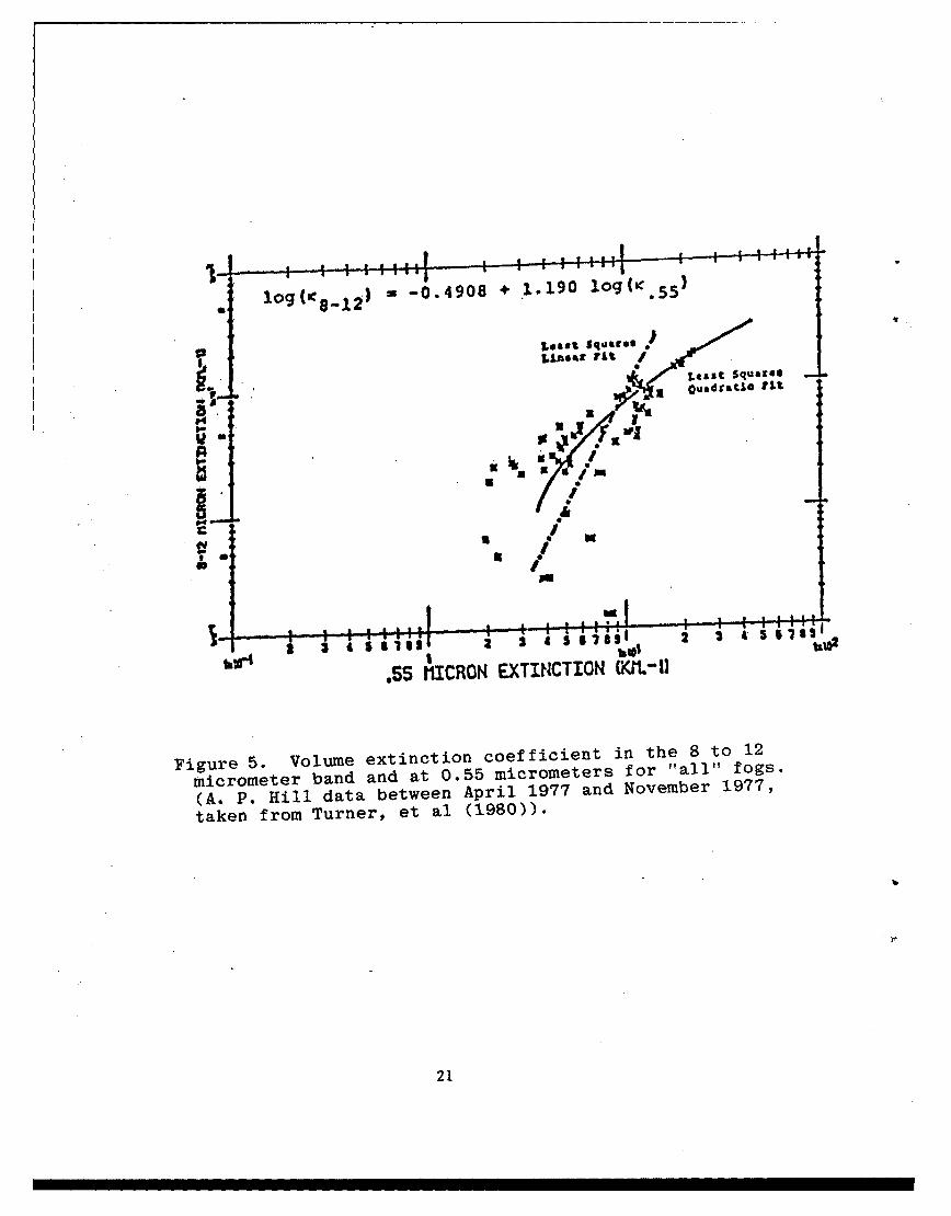
3..-I -1,fl.-0490 +'ICO F.XINTOg KI.L'

(A. P.Hl dt ewenArl 97ad oe ral fit7.S5 ~ MICRO EXTNTINM1

taken from Turner, et al (1980)).

21

U S 0ll llll lll I I Il Il i llll lilll ll llll lili i ll

0 l 8 -1 2 ) - -2.439 + 2.920 1og(K. 5 5 )

S&east SquaroeS~QuAdCaUS TI

aa

e Loaet Squares

Linear rit

U" IUU

1- 2 t 4 50285 2 3 4 5 aS2 3 4 s 1il

.55 MICRON EXTINCTION (KMl.-t)

Figure 6. Volume extinction coefficient in the 8 to 12micrometer band and at 0.55 micrometers for "dry" fogs.(A. P. Hill data between June 1977 and November 1977,taken from Turner, et al (1980)).

22

, I : , , i i ! I :- I I J t |I I i ll -

log(1c8 - 1 2 ) -0.2881 + 1.062 log,. 5 5 )

Least square$

g Linear --Le t Squat..00AN quadratic lit

JI M

X

I /

U V

.55' MICRON EXTINCTION (KIM.-I)

Figure 7. Volume extinction coefficient in the 8 to 12micrometer band and at 0.55 micrometer for "wet" fogs.(A. P. Hill data between April 1977 and November 1977,taken from Turner, et al (1980)).

23

100

X = 0.6328 jm

n = 1.332 - 1.44x10"7

FORWARD

10o 10

L LJU'"

inestiswthtepatcewais

0 BACKWARD

z PO *0 U,0 00

0 0 PoP 0

0~* 0 0 00 so

10 0.10 0 0

0 0. 10 1 . 2.c.530c.

PATIL RAIU (mm

Figure~~~~~~~~~~ 8.Vraino hefradadbckadsatrnineniie wt te atilerdis

02

The large scatter in the GAP and OPAQUE data results

from combining data from many different fogs into one data

plot. Because fogs are characterized by the particle size

distribution function, and because the ratio of the infrared

extinction to the visible extinction is very sensitive to

particle size, a large scatter in fog extinction data should

be expected when considering many fogs. Another contribution

to extinction is absorption by the air. This contribution is

dependent on weather parameters such as temperature and pres-

sure and must be predicted separately in order to isolate the

extinction due to fog. As Turner, et al (1980) have suggested,

the linear relation between the logarithms of the extinction

coefficients may be a good approximation for one fog. If mea-

surements are made at intervals on the order of a minute in-

stead of at half-hourly intervals, as in the case of the GAP

and OPAQUE data, the extinction of radiation may be studied

as the fog evolves. This is clearly evident from data sampled

at one-minute'intervals at the Keweenaw Research Center (KRC),

which will be discussed below.

OBJECTIVE

The objective of this work is to develop a better

understanding of the propagation of infrared radiation

through the lower atmosphere especially in adverse weather.

The approach consists of a program of experimental measure-

ments and computer modeling combined with a review of the

work of other investigators.

25

RECOMMENDATIONS

For calculating infrared absorption due to molecules,

LOWTRAN should be used.

The model used to compute attenuation of radiation

at a wavelength of 0.6328 micrometers due to rain, as de-

scribed in this report should be used as part of the vehicle

signature model. The transmission in the 8 to 12 micrometer

band may then be computed using data presented here on the

relation between the two extinction coefficients.

A model of extinction by snow as a function of snow-

fall rate and/or liquid water content should be developed by

augmenting the KRC weather station with snowfall measuring

equipment.

A study of extinction by fog based on a method pre-

sented in this report could be made by installing a particle

size measuring system on the KRC transmission range.

Snow phase function measurements at 1.06 micrometers

should be performed.

A 10.6 micrometer laser should be installed on the

KRC transmission range to obtain data for use with CO 2 laser

rangefinders.

26

THEORETICAL FORMULATION

Extinction by particulate matter is in general due to

both scattering and absorption. In order to assess the rela-

tive importance of scattering versus absorption, the complex

index of refraction must be known. Scattering is governed by

the real part of the index of refraction while absorption is

a function of the imaginary part. The phase function f(O,p),

namely the angular dependence of the scattered light, is

usually normalized

w 4= -4 f f(o,0) dQ (8)41T

where 5 is the albedo, or ratio of scattering to total ex-

tinction (absorption plus scattering) and 0 and p are angles

describing the scattering direction in spherical polar co-

ordinates. In practice, scattering is assumed to be indepen-

dent of the azimuthal angle 4 so Eq. 8 may be rewritten

7TS= f f(e) sine do (9)

0

where 0 is the scattering angle. As the scattering parameter

p = 27r r/X (where r is the particle radius and X is the wave-

length of the incident electromagnetic radiation) is increased,

the amount of forward scattering (near 0*) increases, while

backscattering (1800) oscillates, as illustrated in Figure 8

for the case of raindrops illuminated by radiation with a wave-

length of 0.6328 micrometer from a Helium-Neon laser. When

calculating transmission through a scattering atmosphere, an

estimate of the amount of radiation which reaches the detector

after experiencing one or more scattering events must be eval-

uated to determine what order scattering processes are impor-

tant. Because it is a measure of the angular spread of the

scattered radiation, the phase function is essential to an

accurate estimate of transmission in a scattering atmosphere.

27

When calculating the received power of a laser trans-

missometer the relative importance of both scattering and

absorption must be carefully considered. Since some of the

scattered radiation will reach the detector after one or more

scattering events, the receiver parameters must be considered

when evaluating the scattering contribution. The instrument

dependence must be accounted for when either measuring or

using experimental values of atmospheric extinction under

adverse weather conditions such as fog, rain, or snow. The

amount of scattering is dependent on the real part of the in-

dex of refraction while absorption is related to the imaginary

part. For a particle described by a large scattering param-

eter (x >> 1), a very strong forward scattering is observed.

The shape of the particles is also a factor in determining

the phase function. Computations similar to those of Mie

(1908) for spheres have been made for cylinders (Kerker,

1969) and regular hexagonal plates (Jacobowitz, 1971).

The geometry of a laser transmissometer is shown in

Figure 9. A laser with power IL and negligible beam diver-

gence is located a distance R from a receiver described by

a collection optics diameter H and an acceptance angle a R'

The amount of power reaching the receiver without

undergoing a scattering event is given by

1 0 1L g P=NS (R) (10)

where g is a geometrical factor related to the divergence

and profile of the laser beam and the type and size of the

receiver optics. The probability of a photon traveling a

distance R without being scattered or absorbed, PNS (R),can be written

PNS (R) = exp {-[N(os + a A) + 6AIR]R} (11)

where N, a., and GA are the number density, scattering cross

section and absorption cross section, respectively, of the

particles and 6 AIR is the atmospheric extinction coefficient.

28

.- ..0 Receiver

dx U c

R

Figure 9. Laser Transmissometer Geometry

29

The contribution of first order scattering to received power

can be written

1 L fR f P s(x) f(C) PNS (R - x) dQ(0) dx (12)0 NO)

The probability of scattering in the element dx after travel-

ing a distance x is Ps(x) dx where

Ps(x) = Nas PNS(x) (13)

and the phase function f(e) has been evaluated at the scatter-

ing angle c. The solid angle P(c) is limited by the size of

the receiver. The expression for second order scattering is

written as

RR2 = ILf f f f Ps(x) f(y) Ps(x' - x) f(6) PNS(R - x')

2 x Q(y)0(6) (14)

dQ(6)dQ(Y) dx' dx

where the first and second scattering angles are given by Y

and 6, respectively.

As can be seen from Eqs. 12 and 14, the magnitude of

the scattering contributions depends on the phase function.

A critical factor in determining the type of scattering,

hence the required phase function, is the size parameter p.

When p << 1 and ImIp < 1, where Iml is the complex index of

refraction, the scattering is referred to as Rayleigh scat-

tering described by the phase function shown in Eq. 1.

When dealing with spherical particles with p > 0.1,

a rigorous calculation is required. For distributions of

spherical particles the scattering amplitudes must'be calcu-

lated for each particle size using Mie theory (1908) and

averaged over the particle size distribution function. For

very large spheres (p > 10) it is often more efficient to use

geometrical optics to calculate the phase function.

30

In order to compute the attenuation of radiation by

rain, the atmospheric raindrop size distribution function

must be known. Laws and Parsons (1943) have measured the

drop size distribution at the surface. The atmospheric rain

drop distribution may then be determined using the size data

of Laws and Parsons (1943) together with the raindrop fall

velocity measurements of Laws (1941). The results are shown

in Figure 10. The drop sizes considered varied in radius

from 0.0625 to 3.25 millimeters. The phase function and

scattering efficiency of each individual drop size is com-

puted using Mie theory assuming that the drops are pure

water with a refractive index of 1.332 - 1.44 x 10- 8 i. The

composite phase function and cross section of the rain is

found by averaging over the rain drop size distribution

function. The composite phase function and cross section

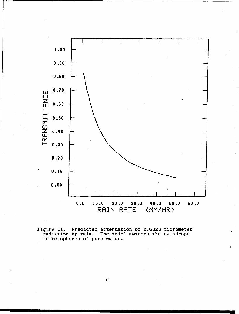
are then used in Eqs. 10, 12 and 14 to compute transmission.

The predicted transmission is graphed as a function of rain

rate in Figure 11.

A linear relation between the logarithm of the extinc-

tion at wavelengths around 10 micrometers and the liquid

water content of fog has been shown by Chylek (1978), Pinnick,

et al (1979), and Carradini and Tonna (1981). Such a relation

may be explained by examining the dependence of the extinction

efficiency factor QE on the size parameter. As shown in Figure

12, the efficiency factor at a wavelength of 10.6 micrometers

may be approximated as a straight line out to a size parameterof 8.0 corresponding to a fog droplet with a radius of 12.7

micrometers. Fog drop size distributions are dominated by

particles of radius less than 7 micrometers (Pinnick, et al,

1979; Carradini and Tonna, 1981; Roach, et al, 1976; Pinnick,

et al, 1978). Using the relation

a E(X,r,m(X)) = QE(Xr,m(X)) r2 = C(X)r3 (15)

31

10

RRIN RATEK Il Isl•i.

' 9.14 W*IiHR: I M. M MhRE

* 16.4 nwiH

--

Z 10 -

U

10- 2

CLC

Z

C:. -3

cy10

10-4

I I , , , 1 1 1 , , , 1 , , I I 11, , ,111

10 102 10 10

RAINDROP RADIUS

Figure 10. Fraction raindrop size distribution.

32

I I

1.00

0.90

0 .80

LLI 0.70UzCI: 0.60I--

. 0.50

0")Z 0.40al:

H- 0.30

0.20

0.10

0.00SI I

0.0 10.0 20.0 30.0 40.0 50.0 60 .0RAIN RATE (MM/HR)

Figure 11. Predicted attenuation of 0.6328 micrometerradiation by rain. The model assumes the raindropsto be spheres of pure water.

33

4.0

UJ 3.0

C0

S.C

"LU 2.0 /• 1/

- Im

1.0 I0.0 LI

0.0 10.0 20.0 30.0

Size Parameter p

Figure 12. Extinction efficiency as a function of sizeparameter. Computations were made for spherical waterdrops using Mie theory.

34

where CMX) is the slope of the curve in Fig. 12 for size

parameters less than 8.0, the extinction coefficient in the

8 to 12 micrometer band may be written

8_12(t) = fl2 CMX)f12.7 n(r,t)r 3dr dX (16)8 0

where the total number of fog particles per unit volume is

given by 0

N(t) = f n(r,t)dr (17)0

The inner integral in Eq. 16 is proportional to the liquid

water content of a fog described by the drop size distribu-

tion n(r,t). Consequently, the extinction in the 8 to 12

micrometer region can be directly related to the liquid water

content of the fog. A similar relation between extinction ef-

ficiency and the size parameter exists at a wavelength of 0.6328

micrometers for fog drops of radius less than 1.0 micrometer.

Because fogs contain a significant number of drops with radii

greater than 1.0 micrometer, the extinction coefficient in the

visible region is a function of both the particle size distribu-

tion and the liquid water content of fog. As a fog forms and

dissipates, the liquid water content increases then decreases,

but the drop size distribution n(r,t) does not retrace its evol-

ution in time, so the path of the data points on the log-log

plot does not retrace its steps. A linear model may be a good

approximation for the dependence of S IR on 8VIS for any single

fog process, but only if measurements are made on a time scale

short compared to fog lifetimes. However, a single line cannot

represent the relationship between IR and 0VIS for fogs in

general, because differences in n(r,t) cause a large variation

in VIS for any given liquid water content.

35

EXPERIMENTAL FACILITY

A sheltered outdoor transmission range has been estab-

lished at KRC, along with facilities to monitor appropriate

weather parameters. The range incorporates a folded path, in

which radiation goes from the outdoor source out a window to

a plane mirror at 500 meters, and is reflected back to the re-

ceiver, which is located indoors near the source. The optical

arrangement is shown schematically in Figure 13. The advantage

of this arrangement, as compared to a straight path, is that

all the electronics are at one end, making calibration, mainte-

nance, and temperature control relatively easy.

Visible transmission is measured by using a Helium-Neon

laser as a source. The laser emits 0.6 mW CW, is mechanically

chopped at 900 Hz, and is aimed at the mirror with no collimat-

ing optics. The receiver for the laser is based on cassegrain

optics 20 cm in diameter with an li-milliradian angle of accep-

tance. The detector is silicon and it is fitted with a narrow-

band filter centered at the laser wavelength, 0.6328 micrometer.

The detector output is fed into a phase-sensitive amplifier,

along with a chopper reference signal. The laser and chopper

are shown in Figure 14, and the receiver optics are shown in

Figure 15.

Near infrared transmission is determined using a neodym-

ium doped YAG laser as a source of radiation at a wavelength of

1.06 micrometers. Because of range safety regulations, the

laser output is attenuated to 1.0 milliwatt before exiting the

laboratory. The beam is mechanically chopped at a frequency of

400 hertz and aimed at the mirror without any collimating optics.

A Cassegrain telescope 15 cm in diameter with a 4-milliradian

field of view is used as a receiver. A silicon detector is

mounted at the focal point. The detector output is fed into a

pre-amplifier and then into a phase sensitive amplifier together

with the chopper reference signal. To guard against errors be-

ing introduced into the transmission measurements by laser power

36

00 tz Chopper

90 zChopper tto

400 hi ChopperDt

Loo*

Fiuea 13.tte Sceai iga ftasis onglabraoy

Eý ] Pase Snsith D37

Figure 14. HeNe Laser and Chopper

38

Figure 15. HeNe Receiver

39

fluctuations, the output of the Nd:YAG laser is continuously

monitored. The laser and chopper are shown in Figure 16 and

the receiver is shown in Figure 17.

The apparatus used for the infrared measurements is the

Barnes Engineering Transmissometer System, Model 14-708, which

consists of a source unit, a receiving unit, and a data logger.

The source is a temperature controlled black body with chopper

and optics, the receiver consists of a 4-inch diameter germanium

lens focussing the radiation on a detector, in front of which is

one of four infrared filters mounted on a wheel, and the data log-

ger, containing a phase-locked amplifier, provides both digital

and analog measures of percent transmission over a one-kilometer

path. The source and receiver are shown in Figures 18 and 19,

respectively. The Barnes Transmissometer has been modified to

change channels under computer control. This enables data col-

lection in both the 3 to 5 and 8 to 12 micrometer bands almost

simultaneously.

The mirror which is located 500 meters from the building

is 20 cm in diameter, optically flat, and is coated with alum-

inum plus a protective overcoat. It is in an adjustable mount

on top of a steel column anchored in concrete. The mirror is

sheltered from weather by a tubular shroud, which is mounted

independently of the mirror support column. The sources and

receivers are also sheltered from weather, by an extension of

the building.

Transmission data is recorded both on strip charts and

digitally. The digitizer is controlled by a microcomputer,

which also processes the data. Outdoor transmission measure-

ments are modulated by refractive scintillation, which depends

on weather conditions in a complicated way. To arrive at a

value of transmission typifying a given time interval, the

signal is digitized many times, and the individual samples

are averaged to obtain the mean value. To record a measure

of the size of refractive scintillations, the standard devia-

tion of the samples is also calculated and recorded. Data are

40

Figure 16. Nd:YAG Laser and Chopper

41

Figure 17. Nd:YAG Receiver

42

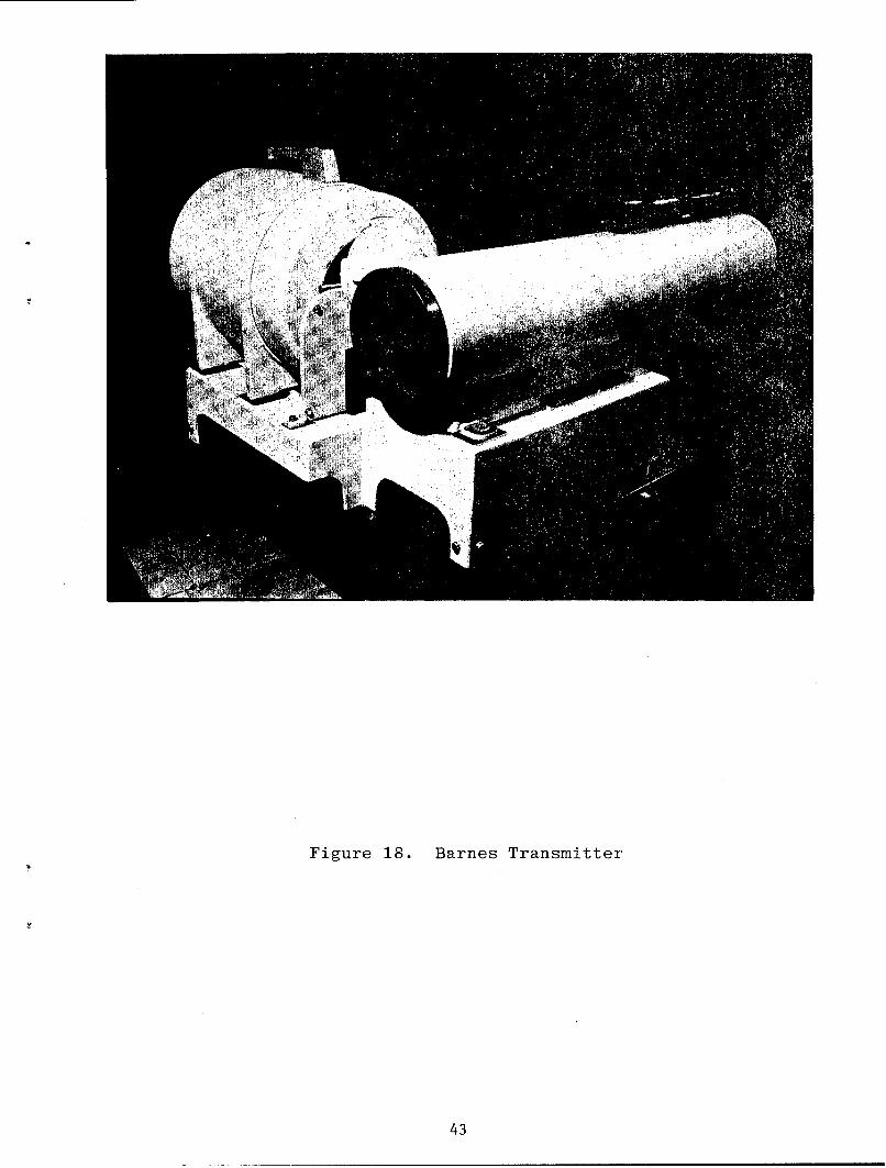
Figure 18. Barnes Transmitter

43

Barnles Pecei~ver

44

then stored on a floppy disk, and can be examined later on a

video display, in a transmission-versus-time format which sim-

ulates a strip chart. Interesting time intervals are then

further analyzed and plotted on a digital plotter. The micro-

computer system has been interfaced to the Michigan Technologi-

cal University's UNIVAC 1100/80 computer. The data files are

transferred to the UNIVAC for further processing and storage.

Weather data are necessary to characterize the path

during field experiments. For this purpose, a weather station

(shown in Figure 20) has been established at KRC, which auto-

matically records the parameters listed in Table 1 in a digi-

tal format, at pre-set time intervals. Besides the standard

weather variables, it will be necessary to characterize fall-,

ing snow for future experiments. This task will be accom-

plished in two ways: by the use of replicas, and by photo-

graphing crystals caught in black trays. Snow crystals will

be divided into six main categories (needles, plane dendritic,

spatial dendritic, graupel, powder snow, and crystals with

droplets) and a given snowfall will be characterized by the

size statistics of each category.

A polar nephelometer, shown in Figure 21, has been

constructed at the Keweenaw Research Center to measure the

phase function of various types and sizes of particles. A

Helium-Neon laser operating at a wavelength of 0.6328 micro.-

meters is used as a light source and two photomultiplier tubes

mounted on movable arms are used as detectors. Snow crystals

are brought through a vertical chute leading from the roof to

the scattering volume located above the pivot of the two arms

by creating a slightly reduced pressure in the laboratory.

The rate at which particles are brought into the scattering

volume is controlled by regulating the pressure gradient be-

tween the room and the outside. Scattered light is collected

by a lens placed in front of each photomultiplier and focussed

onto the photocathode. The reference arm is placed at an angle

150 while the measurement arm is used to measure the phase

45

St w

Figure 20. Weather Station

46

Table 1. KRC Weather Station

Weather Parameter Measuring Instrument

Air Pressure Analog Output Barometer

Air Temperature Thermocouple

Air Temperature Gradient Series of Thermocouples

Asphalt Temperature Thermocouple

Fog Visiometer

Ground Temperature Thermocouple

H20 Vapor Density Optical Dewpointer

Net Solar Load Radiometer

Rainfall/Snowfall Tipping Bucket

Smoke & Dust Nephelometer

Wind Direction Wind Vane

Wind Speed 3-Cup Anemometer

47

S....I - -- LA S E RD

Figure 21. Polar Nephelometer. The laser beam is expandedby a beam telescope (B) and encounters the snowflakes atthe intersection of the two movable arms. The scatteredlight is collected by lenses (L) and focussed onto thedetector (D). The reference detector is placed at er forthe entire experiment while the measurement arm is usedto measure the phase function at angle es. Polarizationmeasurements may be made by placing polarizers (P) afterthe beam telescope and in front of the collection lens onthe measurement arm.

48

function. As a snowflake falls through the laser beam, a

pulse is observed at the output of each phototube. Coinci-

dence of pulses from both the reference and measurement

phototubes is used to ascertain that the snowflake did pass

through the scattering volume and not a part of the laser

path visible to only one photomultiplier. To insure that

the snow crystals do not change phase during the experiment,

the room is allowed to cool to the outside temperature.

RESULTS

Because water vapor is an absorber of infrared radia-

tion, it is important to know the transmission losses due to

water vapor and other atmospheric molecules as a function of

temperature, atmospheric pressure, and relative humidity.

This is easily calculated with repeated application of LOWTRAN

using a filter function comparable to those of the Barnes

transmissometer. The results are plotted as a function of

temperature in Figure 22 for the 3 to 5 micrometer region for

various values of the relative humidity at an atmospheric pres-

sure of 1000 millibars. Similar curves are obtained for other

values of the atmospheric pressure. A maximum attenuation of

34% is obtained at a temperature of 340C and a relative humid-

ity of 100%. A more dramatic decrease in transmission with

increasing relative humidity is seen in the 8 to 12 micrometer

band as shown in Figure 23. An attenuation of 76% is predict-

ed for a temperature of 35*C and a relative humidity of 100%

at an atmospheric pressure of 1000 millibars.

The attenuation of Helium-Neon laser radiation of wave-

length 0.6328 micrometers by rain has been measured as a func-

tion of rain rate (Winchester et al., 1982). Both transmission

and rainfall were averaged over 1-minute intervals. The re-

sults are shown in Figure 24 superimposed on the theoretical

49

35 PReSSURE: 1000MB3-5 MICROMETERS

85 RLTVZ HUMIDITYIo 80

U) 75 2- toy

Z 65 Tlo

~60

55

TEMPERATURE (C)

Figure 22. Predicted transmission in the 3 to 5 micrometerband. The curves were obtained using LOWTRAN for clearair.

50

100 . - .

90

"" 80 "

z tIrlI"01tT~o 60

50 3- fO0(.4 2- q 0 IS~~q- f

V) 6- SolZ 30

S20

10 PRESSURE: 1000MB8-12 MICROMETERS

OI'

TEMPERRTURE (C).

Figure 23. Predicted transmission in the 8 to 12 micrometer

band. The curves were obtained using LOWTRAN for clear air.

51

1 .00

0.90

0.80

UW 0.70

za: 0.60I- -

. 0.500")X

Z 0 .40a:

I- 0.30

K K

X

0.20

0.10 X X

0.00I I I I II

0.0 10.0 20.0 30.0 40.0 50.0 60.0

RAIN RATE (MM/HR)

Figure 24. Comparison of experimental data and theoreticalmodel for extinction of 0.6328 micrometer radiation byrain. The data were collected and averaged over 30-secondintervals.

52

curve described previously. The agreement between the model

and experiment is quite good for rain rates greater than 10

millimeters per hour. At rain rates less than 10 millimeters

per hour, good agreement between theory and experiment is ob-

tained only if the lower rainrate occurs initially or is im-

mediately preceded by a period of intense rain. After a

period of constant rain at rates less than 10 millimeters

per hour, the experimentally measured value is much less than

the predicted value. This is attributed to the suspension or

near-suspension of some of the very small drop sizes associated

with low rain rates in the atmosphere.

In order to develop a similar model for attenuation of

visible laser radiation by snow, it is necessary to know the

phase function and the absorption and scattering cross sections

of snowflakes of different shapes and.sizes. A model for the

phase function of snow needles has been developed (Winchester,

1982a and b) and found to be in good agreement with previously

measured data (Winchester et al., 1981). The phase function

of natural snow crystals was measured during an intense snow

storm on November 15, 1980. The measurements were made with

unpolarized light since a complete set of polarized measure-

ments would require at least four hours. Data were taken be-

tween 100 and 1700 in 50 intervals. At each scattering angle,

a minimum of 51 events were recorded. Ice crystals were col-

lected and examined after every fourth set of phase function

measurements. The crystal size and shape remained constant

during the two-hour experiment. The crystals were needles

with an average length of 2.1 millimeters and an average

radius of 0.125 millimeters corresponding to a size parameter

of 1266. Very little riming was observed. Comparison of

crystal size and shape measurements in the laboratory and

outside showed the system which delivered the crystals to

the scattering volume had no effect on crystal size or shape.

The needles fell with their axes oriented in a vertical

direction.

53

The phase function of the snow needles shown in

Figure 25 has four distinct features: a forward scattering

peak, two broad lateral scattering structures between 700

and 1150 and between 115' and 150', and a backscattering

region at angles greater than 1500. The phase function

values were determined by averaging the measurements at each

scattering angle and then normalizing at 100. The standard

deviation at each point is plotted as an error bar. The

phase function in Figure 25 shows a deeper minimum and less

lateral scattering than the measurements of Huffman and

Thursby (1969). This is consistent with the snow crystals

observed in this study being much larger than the artificial

ice crystals used in all other studies as more energy goes

into forward scattering for larger particles. A broad back-

scattering feature present at angles greater than 145* may

contain an icebow.

As several investigators (Huffman and Thursby, 1969;

Huffman, 1970; Dugin et al., 1977) have reported, Mie theory

cannot be used to describe the phase function. Liou (1972a)

has developed a straightforward method for computing scat-

tering from circular cylinders. Using this method the phase

function of a circular cylinder of ice with a complex refrac-

tive index m = 1.332 - 1.44 x IO 8 i was calculated at a wave-

length of 0.6328 micrometers. The wavevector of the incident

radiation was assumed to be perpendicular to the cylinder

axis and the scattered intensities were summed over all pos-

sible polarization combinations. The resultant, shown in

Figure 26, has been averaged over a 50 collection angle and

normalized at 100. The exact calculation using the method

of Liou (1972a) predicts much more scattering between 100 and

400 and icebows at 1430 and 1680. The computed phase func-

tion has some structure between 700 and 1300, but it does not

match the structure shown by the data. The general intensity

level of the lateral scattering does agree with experiment as

does the intensity of backscattering near 1600.

54

10, -

100 1

zI L

UJ zX

Tx

X x--

1. x'V 'I.;.;; I. I x

10-' xIrX TX X X T x X'X X ±.T x~j

10-3

0 90 180

SCATTERING ANGLE

Figure 25. Phase function measurements of snow needlesnormalized at 100. The crystals averaged 2.1 milli-meters in length and 0.125 millimeters in radius.

55

1 1lI I~ I IlI I I I II I I I

105

10'

103

zO 102

I"IQzM 101

Ia.ILl

Ui

"i" 1 0 .

10"0.

I -,I I I I .I I I I

SX

10-1

0 90 160

SCATTERING ANGLE

Figure 26. Comparison of experiment with calculatedphase functions. Scattering from circular cylinderswas computed using the method of Liou (1972a) whilethe geometric optics approximation sums the diffracted,reflected, and refracted components.

56

Several ray tracing methods have been reported for

hexagonal platelets and hexagonal columns (Jacobowitz, 1971;

Wendling et al., 1979; Liou and Coleman, 1980). These

methods follow the internal path of a ray inside the ice

crystal for up to six internal reflections. Since natural

ice crystals such as snow are formed by successive deposi-

tion and scavenging it is reasonable to assume that each

crystal is made up of many small domains. In the case of

needles, some of the domains may be annular, resembling

the rings of a tree. There is considerable scattering and

absorption of light, as well as polarization scrambling,

at the domain interfaces. This can explain the difference

between the measurements of depolarized light components

and computed values of Fresnel coefficients observed by

Sassen and Liou (1979a and b). A ray tracing model for a

circular cylinder oriented with the cylinder axis vertical

was used to obtain a geometric optics solution for the

phase functions. The method follows each ray path through

the crystal and assumes that radiation not exiting the

crystal on the first pass is absorbed. The externally re-

flected and transmitted components are studied for 6000

equally spaced rays incident on the cylinder. A single

rectangular diffraction pattern (Born and Wolf, 1970) is

then added to give the phase function which has been nor-

malized at 100. The resultant is shown as the dashed curve

in Figure 26. The agreement between the ray tracing solu-

tion and the data is quite reasonable at scattering angles

less than 1400. In the geometrical optics approximation

the backscattering from a cylinder is concentrated near

180* instead of in a broad peak as seen in the data. The

broadening of the backscattering is attributed to surface

roughness and end effects.

The comparative extinctions at 0.6328 micrometers,

1.06 micrometers, and in the 8 to 12 micrometer bands may

be illustrated using GAP-type plots. However, when using

57

GAP-type plots, it should be remembered that the susceptibility

of the receiving optics to scattered radiation influences the

extinction coefficient used in these plots. The He-Ne laser

receiver has a field of view of 11 milliradians while the

Nd:YAG laser receiver has a 4-milliradian field of view. The

field of view of the Barnes transmissometer is also 4 milli-

radians. The effect of field of view on susceptibility to

scattered radiation has been discussed previously (Winchester,

et al, 1981).

As described previously, attenuation of radiation in

the 8 to 12 micrometer band by fog is a function of the liquid

water content of the fog while attenuation at 0.6328 micro-

meters is related to the fog droplet size distribution func-

tion. This is shown by the behavior of the infrared and

visible extinction coefficients during a period of fog ob-

served on 14 April 1980 (see Figure 27). As the fog formed

a linear path is traced out (0) as the liquid water content

increases. This process lasted 76 minutes and was sampled

at one-minute intervals. The fog then began to dissipate

over a 63-minute period (3). During this time interval, the

liquid water content of the fog decreased. The fog forma-

tion and dissipation extinction data do not lie along the

same curve because the particle size distribution function

is not a simple function of liquid water content. As the

fog again thickened over a 39-minute period, a third path

(A) is parameterized by the two extinction coefficients.

Figures 28 and 29 show the extinction coefficient in

the 8 to 12 micrometer band as a function of the extinction

coefficient at 0..6328 micrometers for fogs measured on 7 June

1981 and 8 June 1981, respectively. These two graphs are

typical of the many fog measurements made during the course

of this study. When data from many fogs are graphed on the

same plot, the value of the infrared extinction coefficient

may range over a decade for a single value of the visible

extinction coefficient (Turner, 1980). This problem is

58

"I I " ' ' " " I 1... .. I I "I l'II

10 -

0

LA

S10oAE

oo2 m_

040

100

I i i I i ,, , , , I i ,, ,1 , , ,

10" 10° 10'

Figure 27. Extinction fog, 14 April 1980. Fog extinction

measurements were obtained at one-minute intervals. Theextinction coefficient in the 8 to 12 micrometer band isplotted as a function of the extinction coefficient at0.6328 micrometers. The fog formed over a 76-minute per-iod (0), dissipated over the next 63-minute period (U),and then thickened again (A) over a 39-minute period.

59

I I I I I I I Ij I I I I 111"

10.

zo -FOG07 JUN 1981

U

F-XLLI

X*f

10 X

101'10 .. 10

Fiue2. xiio nFg 7 Jue191

10 60

LL I X Ii~~ ~ l 40Ii0'ICD32 MIRMTRETNTO

10-0

I 1I " Ii I I ' ' 11" I

10z

c FOG1--- -VA

F- 08 JUN 1981 dXXX

LU

LU X

b-t

H-N

X

LL- 0X

L XX -

CD

-!j

10--

I I I I , , , , , I I I I 1 1, , , I

10"1 10 10

0.6328 MICROMETER EXTINCTION

Figure 29. Extinction in Fog, 8 June 1981.

61

compounded by sampling at thirty-minute intervals as has been

past practice. By sampling at one-minute intervals the con-

tinuous change in the GAP-type curve may be observed. This

is best illustrated in Figure 27 and can also be seen in Fig-

ures 28 and 29. The spread in parameterized curves observed

over many fogs is due to the variations in the fog droplet

size distribution function.

When measuring the extinction coefficients at 0.6328

micrometers and in the 8 to 12 micrometer band by rain, it

is important to include the susceptibility of each instrument

to scattered radiation. Rain drops are large compared to the

wavelengths of radiation considered here and the phase func-

tions will be dominated by an intense forward scattering peak.

If the complex index of refraction of the rain drops is as-

sumed then almost all the visible radiation is scattered with

only a very small amount being absorbed while the scattering

and absorption contributions to extinction are approximately

equal in the infrared band (Winchester, et al, 1981). Com-

parison of the measured extinction coefficients due to rain

is shown in Figure 30. Both extinction coefficients graphed

in Figure 30 include other losses such as absorption due to

atmospheric gases and water vapor and are not corrected for

scattered radiation. The data for 6 June 1981 are typical

of extinction data by rain.

Because of an average annual snowfall of over six

meters, extinction of visible and infrared radiation by

falling and blowing snow may be studied extensively at KRC.

Transmission measurements were made at 0.6328 and 1.06 micro-

meters and in the 8 to 12 micrometer band. As mentioned pre-

viously, the three transmissometer systems are susceptible to

scattered radiation to different degrees. Therefore the GAP-

type curves parameterized by the observed extinction values

depend on the phase function of the scattering particles. A

change in the type or size of the scattering particles will

affect the slope and position of the parameterized curve.

62

I II I 1 I iiiI I I 1 111I111I

10 -

0RAIN

U.) 6 JIJN 81-Zl-.-

XH-

LLJ

H- 10 0

0

C-)e--

cOJC")(.0

CD

10-1

I , , , , , , , II , I I , ,I

10-1 10 0 10 1

8 - 12 MICROMETER EXTINCTION

Figure 30. Extinction in Rain, 6 June 1981.

63

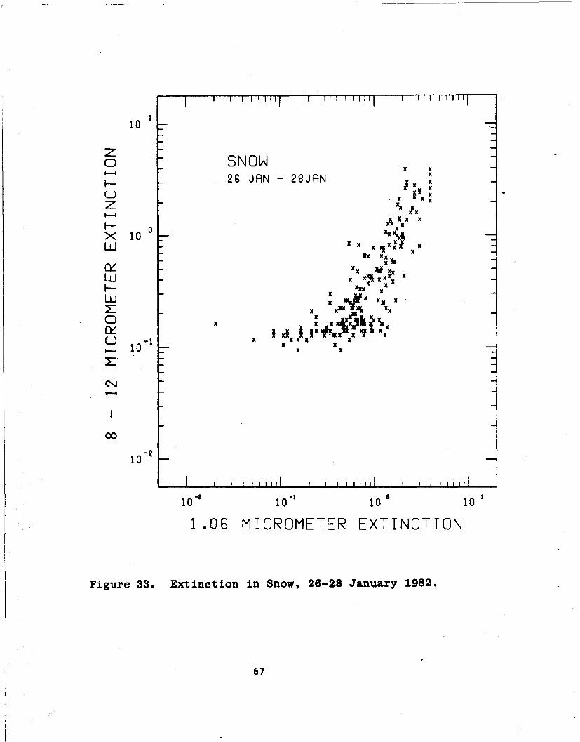
When data collected over a period of several days is

plotted on a single graph, a large spread in the data is

present as shown in Figure 31 for data taken between 26 and

28 January 1982. The spread in the data is due to the pres-

ence of several different crystal types during the three-day

period. This is very similar to the curves of Turner, et al

(1980) for fog. The same behavior is seen in a plot of the

1.06 micrometer extinction as a function of the 0.6328 micro-

meter extinction shown in Figure 32 and in a plot of the 8 to

12 micrometer extinction as a function of the 1.06 micrometer

extinction shown in Figure 33. When dealing with one type of

crystal the spread of the extinction coefficient in the 8 to

12 micrometer band for any given value of the extinction co-

efficient is reduced considerably as shown in Figure 34. The

data were taken in blowing snow over a seven-day period. Blow-

ing snow consists of very small broken snow crystals resembling

needles or bullets with well-defined scattering properties.

Similar results are shown in Figure 35 where the extinction

coefficients at 1.06 micrometers and at 0.6328 micrometers

are plotted. Figure 36 illustrates the behavior of the extinc-

tion coefficient in the 8 to 12 micrometer band as a function

of the 1.06 micrometer extinction coefficient. Again the spread

of the data is reduced.

On 10 February 1982, transmission of 0.6328 micrometer

radiation and transmission in the 8 to 12 micrometer band was

measured in snow consisting of plate-type crystals. The data

snown in Figure 37 lie in a narrow region when plotted on a

fully logarithmic axis. The spread in data for high extinc-

tion values correspond to a time period which included some

blowing snow.

On 20 February 1982, extinction measurements were

made using all three transmissometer systems during a snow-

fall which consisted of planar dendritic crystals. A linear

64

10

0 SNOW /.I--,I -- X X:XXX X ,

26 JAN - 28JAN XIxxF- X

z )K K

1- X:*X 10 K K•

-- X X X I

LdK )I KKX K

-- X XX ~KY- IK xK I •

LLJ X X X xH 4 xW

r K ljK K KKK I

0" X ,f x j ý Xx• x x

K KXKj~f K K Xf

U- X X X XX X

C....) - 1 K x t A. 10 -- K K x_1. 1 X X .

00

i0-2

I0"ii~ I0 eIIIII I 01111

10t 10' 10 10


Figure 31. Extinction in Snow, 26-28 January 1982.

65

101

z SNOW0 26 JAN -28JAN XX, X~ XX

X- X X XX X

F- X( Xz X

Z XX AX'w XXX

10 Al XXXXXX1 JX

X X X XX

XZX X X X XX

C.. 10 X XXX X

CK X )k

0 X0

U

X X

10' 10'1 10 0 10 1



66

10

zo SNOW x x

F-26 JAN -28JAN

>< 10 KK

LLJ XX X X M x Kg X

WU xxt X X

(2 -= KK K

0 10 K .

CoA

10-2

I~~~~~~~L I IIIt 1111I 111

10' 10-1 10 a 101



67

10 1

zo BLOWING SNOWI- 28 JAN- 03 FEB

uj X0 - X-,,x-

10 "

xXwU A

LU XK K

(.3 -1

P_- 10

Cj

0-2

I , I ,, I I 1 1 1 I Iw I, , , , , ,

10-1 10 0 10


Figure 34. Extinction in blowing snow, 28 January -

03 February 1982.

68

11 0 -7 :

z BLOWING SNOW28 JRN - 03 FEB

SX XX

z xX ll xXE

X1 X 1 N

x XX X WX X XLLJ x XX xx X xfllx x

L.. 10 0 X x

LU _ x IxXC X

0

-.0

-I

10.-i

I I i I i i l i I i i i i i l i

101 100 101



03 February 1982.

69

I I ' ''"I11 ' ' I 11 ' " I

10

zo BLOWING SNOWI 28- JRN -03 FEB XX

m x

10 xv

- K K

XXX X

Lii _x ixK

I XXX X X

0 x1

12

I , , , , ,1 ,,I , , , , 1 1 1

10" 10 101



03 February 1982.

70

II I ' I I

10 1

.- SNOWXX X1-- 0 FEB 1982 i&x ,X _

--) - I .xx I

z _F--

XLLJ

L LJ1 I0 xi X

00

00

101-

10 0 101


Figure 37. Extinction in snow, 10 February 1982.

71

relation between the 8 to 12 micrometer extinction coeffi-

cient and the 0.6328 micrometer extinction data is quite

evident in Figure 38. The spread in 1.06 micrometer extinc-

tion shown in Figure 39 as a function of the value of the

extinction coefficient at 0.6328 micrometers is much larger'

than that shown by the 8 to 12 micrometer extinction data.

The spread in the data decreases as the magnitude of the

extinction coefficients increase. A similar curve is shown

in Figure 40 where the 8 to 12 micrometer data is plotted as

a function of the 1.06 micrometer extinction coefficient.

The spread in the data shown in Figures 39 and 40 is attri-

buted to the measurements at 1.06 micrometers. This phenom-

ena was observed repeatedly. On 21 February 1982, Figures

41, 42 and 43 are GAP-type plots of the extinction data mea-

sured in falling snow which consisted of large planar den-

dritic snow crystals. A large spread in the data associated

with the 1.06 micrometer extinction coefficient is seen. On

the next day, 22 February 1982, a variation in the 1.06 mi-

crometer extinction coefficient was seen for needle-type

snow crystals as shown in Figures 44, 45 and 46. In Figures

47, 48 and 49, extinction measurements made in a storm con-

sisting of large needle-like crystals approximately 3 milli-

meters in length show a large spread in the data which is

again attributed to the measurements at 1.06 micrometers.

The large spread in the 1.06 micrometer band is rarely

seen at 0.6328 micrometers or in the 8 to 12 micrometer band

extinction data. This phenomena will be discussed below.

The linearity in the plots of the 8 to 12 micrometer band

extinction data, as a function of the 0.6328 micrometer ex-

tinction, are to be found for all types of snow crystals

when the types are considered singly. This is illustrated

by Figure 50 for snow consisting of needles, Figure 51 for

platelets, Figure 52 for needles, Figures 53 and 54 for

planar dendritic, Figure 55 for needles and Figure 56 for

72

10 1

zo SNOWF- 20 FEB 1982 x X

,, -XXX Xz XXXX OXX

H- (O0

10 0

CD

C-)i

10-1I I I I 1 , 111 I , I I II I

10 100 101



73

101

z SNOW2 20 FEB 1982

U I X

z ,

X X

LUJ

10

0

U

CD

10-1

LJI -I 1111

10' 10 10



74

III II f i l l

10 -

zo SNOW

2" 20 FEB 1982 x X,- aU X

z IF-

LUJ

-10

co-

10 --

10 "' 10 0 10 1

1.06 MICROMETER EPTINCTIOnj


75

JI I I , 111'11 I I, I ,I 111

10 1

zo SNONP-.-4 21 FEB 1982

UzF-

LU t

LL)F- 10

LUC.J

00

ZK

10-1

II 1 1 1 t

10-1 10'0 10'

0 .6328 MICROMETER EXTINCTION


76

" I 1 . . . . - I- , ' 1 . . . I ... ' , 1 ' " 1

10 -

z SNOW2 21 FEB 1982

I.-4

HX

LU

z - -,;b-X

xLLJ

Lij 10 0 _ X-

LLJ X

I -

0•-

U

CD

10-1I • I , , , , , , , , , , , , , , , I

10Oa 10 ' 101



77

10

0 -SNOW21 FEB 1982

z X

.xJX XF

LUJ10010 1

Li

o

-10

1001

1.06 MICROMETER EXTINCTION.-


78

I I i'I 111111 I , I 11(" 11l

10 121.

Zo SNOW

S2 FEB 1982 X x(- MXXX K XzMX

Z X(XM X

w I

X

X

x LU

LLI 10

0 10

L.i

-1

I t I , I I 11 1 I~, I I I 11 1 .

10" ' 10 *

10



79

10

z SNOW

S22 FEB 1982 x x

F--

X -

LUJ

LUJ 10 0

L)

CD 1 10

(.0

101-

I I , , , , , , , I , , 1 , 1 , , , I

10"' 10 ' 101



80

I I I 1 1 1 "1 I I ... ,--,.-I ,

10 1

zo SNOW0-4 22 FEB 1982

LU

z,_ lX x

• xF- 4X

x

C--)

z N'

1- 100

1!.06 MICROMETER EXTINCTON


81

I I I I I I I I I I I I I I I

10

zo SNOW

23 FEB 1982(.3

z

X -

z xx

LUJ

LU-10

LUJ

CD

101

I ' i li. , i I , , 1 1

10"1 10 0 101



82

I , ,, , , , , ,j I , , , , , ,I1

10 -

z SNOW- 23 FEB 1982

I--

L.LJ-

W-Uw

Co

C:)

10- 1

101

I , I , , , I 1 1 .I.. . ,L

10"1 10 0 10 1



83

10

0 SNON

23 FEB 1982

zXx x

LU10 0

LUJ

CD

z

00

10

10- 10i 10

.0' MICROMETER EX,'T "IN TION


84

r I I 11111I I I I 11I111

10

z0 SNOW

24 FEB 1982UzF-XLJ

LUJ SI0 0 _U-io

LU

Co

10- 1

SI I , II

10" 10 10

0.3223 MICROMETER L\'TIkCITTONl


85

10

o SNOW-- 27 FEB 1982OC-)zX-

Ld

LI I-- tOo 0

LU

CoJ"-oCO

S I I I I , 1111, i I I III* l

10" 10 10

0.6328 MICROMETER" EXTINCTION


86

10 1

zo SNOW0 1 MAR 1982 4

LU

z X

,X •

WN

CJ

10 0

S" I I X X

X

to-

l I ~~~I I LAi'l i I ,il

10 "* 10 a 10


Figure 52. Extinction in snow, 01 March 1982.

87

10

o -SNOW--- 03 MAR 1982UZ

I--XLLI

.- 10

LU

00

C-)

10

I * I 11111 Il l , i i 1 ,1

10" 10' 10



88

r I* f I I tI I I I r I I I I

tO

z

o SNOWI-- 09 MAR 1982U XzI---xLLJ

LIU-- 10 0Ld3--

U 'NX

NAN.X

la

Co w

101

S.. ..I , i I 1. i 111 I , I 1 ,,1

10"1 10 10

V..2. MV CROMETER EXTINCTION


89

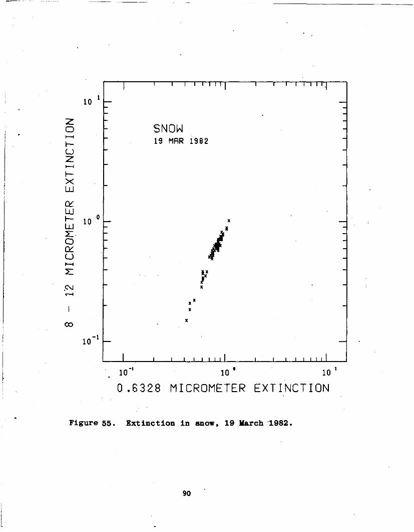
I I I 1 1 1 1 1 1 1 I I 1 1 1 1 1 1 . 1 -l

10

0 -SNOWt 4 - 19 MAR 1982F-U

Ljj

z

n-

0

CD/

00:

I,-I

.•N N

10-1

. I I I , 1 ,1 .1 I I I , , , , ,

10" 10' 10



90

I ! I 1 111 I ! ii|

10

zo SNOW

20 MAR 1982 xx xS" XX X X(3 xxxx

ox

X XLLJ

LLJF- 1o 0_

LU-

c-

10

1 ,I I I

10"1 10 f 10



91

platelets. The slope of the curves depends on both the phase

function of crystals at the wavelengths of interest and on the

susceptibility of the transmissometer receivers to scattered

radiation.

The spread in the transmission data for small values

of the extinction coefficient (less than 1.0 km- 1 ) has been

attributed to the extinction measurements at 1.06 micrometers.

Since the output of the Nd:YAG laser has been found to vary

by as much as 20%, the output is continuously monitored and

the return power is ratioed by the input power. Therefore,

laser power fluctuations are not the cause of the spread.

It is possible that the phase function of snow is consider-

ably different than the phase functions at 0.6328 micrometers

and in the 8 to 12 micrometer band. If the liquid water as-

sociated with snow crystals was having an effect on the phase

function at 1.06 micrometers, a variation in the phase func-

tion may be expected within any given snow crystal type.

However, a similar effect should be seen in the 8 to 12 mi-

crometer band because of the higher imaginary index of re-

fraction of water in this band.

When the extinction due to two types of natural ob-

scurants is measured, a larger data spread is found as is

curvature of the parameterized GAP curve. Measurements of

extinction in the 8 to 12 micrometer band are graphed as a

function of the extinction at 0.6328 micrometers in Figure

57. The evidence of a fog formation and dissipation can be

seen in the data of 10 June 1981. The curvature is attrib-

uted to simultaneous rain and fog in amounts varying in time.

Varying amounts of rain and snow on 31.March 1982 account for

the behavior seen in Figure 58.

92

I IIII I I I I.1 11

10 --

o RAIN & FOGI-- 10 JUN 1981

I"-X

LJ

H.10 0

II -

co

10

i0-I

, I I I I I t J I I I I , , 1 ,

10" 100 101


Figure 57. Extinction in rain and fog, 10 June 1982.

93

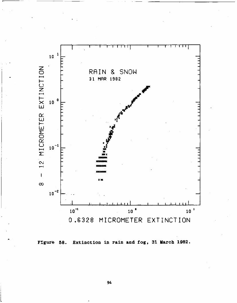
'1I i i i i i11,1 I 1 , ,,1 1 I

10 1

zo RAIN & SNOWI-' 31 MRR 1982

z -u

H--

X 10Lii

LUJ XXXX

Ld - -

0 X1~C3

2 -1 XXS10 M

CJ --_ , _ uum w=x

10-2

,I I I I I I l l I I I I I I I l

10110 1 101


Ftgure 58. Extinction in rain and fog, 31 March 1982.

94

REFERENCES

Asano, S. and G. Yamamoto, Appl. Optics 14 29 (1975).

Barteneva, O.D., Dougyallo, Ye.N., and Polyakova, Ye.A.,Tr. GGO (1967).

Best, A.C., Quart. J. Ray. Meteorol. Soc. 76 16-36 (1950).

Bisyarin, V.P., Bisyarina, I.P., Ruback, V.K., and Sokolov,A.V., Radio Eng. Electron. Phys. 16 1594-1597 (1971).

Born, M. and E. Wolf, Principles of Optics, 4th Ed.,Pergamon Press, New York, 1970.

Bruscaglioni, P., Optics Commun. 27 9-12 (1978).

Bruscaglioni, P., Lett. Nuovo Cimento 24 485-488 (1979).

Bruscaglioni, P. and A. Ismaelli, Nuovo Cimento IC147-166 (1978).

Bruscaglioni, P. and A. Ismaelli, Optica Acta 26 679-691

(9179).

Carradina, C. and G. Tonna, Atmos. Environ. 15 271 (1981).

Chu, T.S. and D.C. Hogg, B.S.T.J. 47 723-759 (1968).

Chylek, P., J. Atmos. Sci. 35 296 (1978).

Dugin, V.P., B.M. Golubitskiy, S.O. Mirumyants, P.I. Paramonov,and M.V. Tantashev, Izv. Atmos. Ocean.__Phys. 7 581 (1971).

Dugin, V.P., O.A. Volkovitskiy, S.O. Mirumyants, andN.K. Nikiforova, Izv. Atmos. Ocean.. Phys. 13 22 (1977).

Duncan, L.D., R.C. Shirkey, R.A. Sutherland, E.P. Avara, andH.H. Monahan, ASL-TR-0047 (1979).

Eklund, H., S. Lundqvist, B. Marthinsson, and S.T. Eng,Infrared Physics 18 337-342 (1978).

Fabelinskii, I.L., Molecular Scattering of Light, Plenum Press,New York, 1968.

Greenberg, J.M., A.C. Lind, R.T. Want, and L.F. Libelo inElectromagnetic Scattering, R.L. Rowell and R.S. Stein, eds.,Gordon and Breach, New York, 1967.

Huffman, P., J. Atmos. Sci. 27 1207 (1970).

95

Huffman, P.J. and W.R. Thursby, J. Atmos. Sci. 26 1073-1077(1969).

Jacobowitz, H., J. Quant. Spectrosc. Radiat. Transfer 11691-695 (1971).

Jessen, W., A. Kohnle, H. Hipp, and D.H. Hohn, Infrared Phys.20 175-183 (1980).

Kagiwada, H. and R. Kalaba, Rand Report RM-5537-PR, RandCorporation, Santa Monica, CA, 1967.

Kerker, M., The Scattering of Light, Academic Press, New York,1969.

Laws, J.D., Trans. Am. Geophys. 22 709-721 (1941).

Laws, J.O., and D.A. Parsons, Trans. Am. Geophys. 24452-460 (1943).

Liou, K.N., Appl. Optics 11 667 (1977a).

Liou, K.N., J. Atmos. Sci. 29 524 (1972b).

Liou, K.N., R. Baldwin, and T. Kaser, J. Atmos. Sci. 33553 (1976).

Liou, K.N. and R.F. Coleman in Light Scattering by IrregularlyShaped Particles, D.W. Schuerman, ed., Plenum Press, New York,1979.

McClatchey, R.A., W.S. Benedict, S.A. Clough, D.D. Burch,R.F. Calfee, K. Fox, L.S. Rothman, and J.S. Goring,AFCRL-TR-73-0096 (1973).

Mie, G., Ann. Physik 25 377-445 (1908).

Moulton, J.R., R.J. Bergeman, and M.C. Sola, IRIS Symposium,1976.

Mugnai, A. and W.J. Wiscombe, J. Atmos. Sci. 37 1291 (1980).

Nikiforova, N.K., L.N. Pavlova, A.G. Petrushin, V.P. Synkov,and O.A. Volkovitskiy, J. Aerosol. Sci. 8 243 (1977).

Pinnick, R.G., D.L. Hoijelle, G. Fernandez, E.B. Stenmark,J.D. Lindberg, G.G. Hoidale, and S.G. Jennings, J. Atmos.Sic. 35 2020 (1978).

Pinnick, R.G., S.G. Jennings, P. Chglek, and H.J. Auvermann,J. Atmos. Sci. 36 1577 (1979).

96

Roach, W.T., R. Brown, S.J. Caughey, J.A. Garland, and

C.J. Readings, Quart. J. R. Met. Soc. 102 313 (1976).

Sassen, K. and K.N. Liou, J. Atmos. Sci. 36 838 (1979a).

Sassen, K. and K.N. Liou, J. Atmos. Sci. 36 854 (1979b).

Selby, J.E.A., F.X. Kneizys, J.H. Chetwynd, Jr., and R.A.McClatchey, AFGL-TR-78-0053 (1978).

Shields, F.S., NV&EOL Internal. Memorandum, 1978.

Shifrin, K.S., Scattering of Light in a Turbid Medium,NASA TT F-477 (1968).

Smith, H.J.P., D.J. Duke, M.E. Gardner, S.A. Clough, F.X.Kneizys, and L.S. Rothman, AFGL-TR-78-0081 (1978).

Sokolov, A.V. and Sukhonin, Ye.V., Radio Eng. Electron. Phys.15 2167-2171 (1971).

Turner, R.E., F.G. Gerhardt, J.L. Manning, R.E. Meredith,S.M. Singer, F.G. Smith, and P.C. Vavra, ASL-CR-80-0177 (1980).

Van de Hulst, H.C., Light Scattering by Small Particles,Wiley, New York, 1957.

Volkovitskiy, O.A., L.N. Pavlova, and A.G. Petrushin, Izv.Atmos. Ocean. Phys. 16 98 (1980).

Wait, J.R., Can. J. Phys. 33 189 (1955).

Wendling, P., R. Wendling, and H.K. Weickmann, Appl. Optics18 2663 (1979).

Winchester, Jr., L.W., W.K. Choi, G.G. Gimmestad, S.M. Lee,and P.N. Parks, Poc. 2nd KRC Symp. on Ground Vehicle IRSignatures 1 123-131 (1980a).

Winchester, Jr., L.W., W.K. Choi, G.G. Gimmestad, S.M. Lee,and P.N. Parks, JOSA 70 1561 (1980b).

Winchester, Jr., L.W., G.G. Gimmestad, S.M. Lee, and D.K.Wilburn, TACOM Tech. Report 12612, 1981.

Winchester, Jr., L.W., G.G. Gimmestad, and S.M. Lee, CLEO '82Tech. Digest 1982.

Winchester, Jr., L.W., Proc. Eleventh International LaserRadar Conference, 1982a.

Winchester, Jr., L.W., Submitted to J. Atmos. Sci. 1982b.

97

CommanderTECTAFort Hood, TX 76544

ATTN: ATCAT-CS-STI

Commander 2Picatinny ArsenalDover, NJ 07801

ATTN: ARDAR-LCU-T, Bldg. 24

U.S. Department of Commerce 5NOAA Environmental Research LaboratoryTechnical Reports Boulder, CO 80303

ATTN: Library, R-51

DirectorU.S. Army Materiel Systems Analysis AgencyAberdeen Proving Ground, MD 21005

ATTN: DRXSY-T

DirectorU.S. Army Engineer Waterways Experimentation StationVicksburg, MS 39180

ATTN: Library Branch

CommanderU.S. Army Aviation Test BoardFort Ruck~r, AL 36360

ATTN: STEBF-PO

CommanderU. S. ArmyArmor and Engineering BoardFort Knox, KY 40121

ATTN: ATZK-AE-TE-E

CommanderU.S. Naval Test CenterCode 3941China Lake, CA 93555

Commander 2U.S. Army Mobility Equipment Research and Development CommandFort Belvoir, VA 22060

ATTN: DRDME-RT

CommanderU.S. Army Electronics Research and Development CommandNight Visions and Electro-Optics LaboratoryFort Belvoir, VA 20060

ATTN: DELNV-VI 10DELNV-L 2

DISTRIBUTION LIST

COPIES

CommanderU.S. Army Tank Atuomotive Research and Development CommandWarren, MI 48090

ATTN: DRCPM-FVS 1

DRCPM-M60 1DRCPM-M113 1DRDTA-TSL 5DRDTA-ZSC 30

DirectorDefense Advanced Research Projects Agency1400 Wilson Blvd.Arlington, VA 22209

Defense Technical Information CenterCameron StationAlexandria, VA 22314

CommanderHarry Diamond LaboratoriesAdelphi, MD 20783

ATTN: DRXBO-RAL 1

DELMD-R-CM 1

CommanderU.S. Army Missile CommandRedstone Arsenal, AL 35809

ATTN: DRSMI-TEI 2DRSMI-REO 1DRSMI-REL 1DRSMI-OG 1DRSMI-RPRD 1DRSMI-RRA 1DRSMI-RRO 1DRSMI-RHC 1

Commander 1U.S. Army Electronic Proving GroundsFort Huachuca, AZ 85613

ATTN: STEEP-MT-ST

Director 1

U.S. Army Ballistic Research LaboratoriesAberdeen Proving Ground, MD 21005

ATTN: DRXBR-LB

Commander 2U.S. Air Force Systems CommandWright-Patterson AFB, OH 45433

ATTN: AGM-65, SD65 E

CommanderU.S. Air Force Armament LaboratoryEglin AFB, FL 32542

ATTN: AFATL-DLB 4AFATL/DLODL Technical Library 4

Commander 5U.S. Army Atmospheric Sciences LaboratorysWhite Sands Missle Range, NM 88002

ATTN: DELAS-EO

CommanderU.S. Army Cold Regions Research & Engineering LaboratoryHanover, NH 03755

ATTN: CRREL-RD 1CRREL-RG 2

U.S. National Aeronautic and Space Administration 1ATTN: Chief of Planetary Materials

Lyndon B. Johnson Space CenterHouston, TX 77058

U.S. Army Chemical Systems Laboratory 2Aberdeen Proving Ground, MD 21012

ATTN: DRDAR-CLB-PS

Air Force OSR/NCBoiling Air Force BaseWashington, D.C. 20332

Project manager Smoke/Obscurants 3Aberden Proving Ground, MD 21005

ATTN: DRCPM-SMK

Air Force GL 1Hanscom AFBBedford, MA 01731

Commander 1U.S. Army Combined Arms Combat Developments ActivityFort Leavenworth, KS 66027

ATTN: ATCA-CCC-S

L 0CL R A EPOR T TE CH N IC AL R E POR T · r----- ---- nI II I I I I I I Sand*.., L 0CL R A EPOR T...

Documents

Transcript of L 0CL R A EPOR T TE CH N IC AL R E POR T · r----- ---- nI II I I I I I I Sand*.., L 0CL R A EPOR T...