Kullback Leibler Divergence forBayesian Networks with Complex … · 2 Kasza and Solomon for the...

Kullback Leibler Divergence for Bayesian Networks withComplex Mean Structure

Jessica Kasza†

University of Copenhagen, Copenhagen, Denmark

Patty Solomon

University of Adelaide, Adelaide, Australia

Summary. In this paper, we compare two methods for the estimation of Bayesian networksgiven data containing exogenous variables. Firstly, we consider a fully Bayesian approach,where a prior distribution is placed upon the effects of exogenous variables, and secondly,we consider a restricted maximum likelihood approach to account for the effects of exogenousvariables. We investigate the differences between these two approaches on posterior inferenceusing the Kullback Leibler divergence. The residual approach is considerably simpler to usein practice, and in applications where the exogenous variables are not of primary interestfor estimation, we show that the potential loss of information about parameters and inducedcomponents of correlation which are of interest, is generally negligible or small.

Keywords: Bayesian network, High-dimensional data, Kullback Leibler divergence, Regulatorynetworks

1. Introduction

The estimation of Bayesian networks given a high-dimensional data set is an area of statisticsto which much research has been recently devoted. Bayesian networks are proving useful inbiology, providing biologists with an alternative means of investigating the inner workingsof a cell, see, for example, Sachs et al. (2005). In particular, such models may be used toprovide insight into the ways in which groups of genes are related to one another, and canbe used to guide the experimentation of wet-lab researchers.

While there are many methods available for the estimation of Bayesian networks, thesemay be roughly split into two broad categories: constraint-based methods and score-basedmethods. Typically, these approaches assume that the data set available for the estimationof a network consists of independent and identically distributed samples from a normaldistribution.

In Kasza et al. (2010) score metrics, for use in conjunction with score-based methodsfor the estimation of Bayesian networks, allowing for the inclusion of exogenous variables inthe estimation of Bayesian networks were presented. These score metrics, modifications ofthe BGe metric of Geiger and Heckerman (1994), increase the applicability of score-basedmethods to data sets that do not consist of independent and identically distributed samples,while retaining the assumption of normality. In Kasza et al. (2010), two approaches allowing

†Address for correspondence: Jessica Kasza, Department of Mathematics, University of Copen-hagen, Universitetsparken 5, DK-2100 Copenhagen Ø, DenmarkE-mail: [email protected]

2 Kasza and Solomon

for the inclusion of the effects of exogenous variables were presented. The first approach,which we will term the Bayesian approach, involved placing a prior distribution on the effectsof exogenous variables. The second approach, inspired by restricted maximum likelihoodand termed the residual approach, involved no such prior distribution. Of interest here isthe loss of information associated with the use of the assumption-free residual approach, asopposed to the use of the Bayesian approach.

In Section 2, after a brief review of the score-based estimation of Bayesian networks,the behaviour of the Bayesian score metric as the variance of the effects of exogenousvariables becomes either very small or very large is considered. It is shown that the residualapproach may be thought of as an approximation to the Bayesian approach, and that whenthe variance of the effects of exogenous variables is a priori thought to be very large, theresidual approach is, in fact, preferable to the Bayesian approach.

In Section 3 the posterior distributions obtained under the Bayesian and residual ap-proaches are compared using the Kullback Leibler divergence. It is shown that when theresidual approach is used the loss of information about the full covariance structure of therandom variables becomes negligible as the sample size increases, providing further justi-fication for the use of the residual approach in the estimation of Bayesian networks. Theutility of the divergence is demonstrated in Section 4, where examples, consisting of bothsimulated and biological data sets, are considered.

2. Score-based estimation of Bayesian networks given a data set with complexmean structure.

A Bayesian network B = (G,Θ), Θ = {θ1, . . . , θp}, for a random vector X = (X1, . . . , Xp)T

consists of two components: a directed acyclic graph associated with X, G = (V,E), withV = {X1, X2, . . . , Xp} and E ⊆ V × V , and a set of conditional distributions{f(xi|xPi

, θi)|i = 1, . . . , p}. The set Pi is the set of parents of Xi, and consists of thosevariables Xj such that there is a directed edge from j to i in G: (j, i) ∈ E. The jointdistribution for X may then be written as

f (x|Θ) =

p∏

i=1

f(xi|xPi, θi).

Bayesian networks encode information about the conditional dependence relationships be-tween the variables in X. The directed Markov properties, as described in Laurtizen (2004),for example, allow conditional independence relationships to be read directly from the graphG.

We wish to estimate a Bayesian network for X given a data set d which, in additionto containing n samples of each Xi, also contains information about m exogenous variablesthought to affect these Xi. As described in Kasza (2009) and Kasza et al. (2010), theregression model for sample k of Xi is assumed to be

Xik =∑

j∈Pi

γijXjk +

m∑

r=1

qrkbir + ǫik,

where ǫik ∼ N(0, ψi), qrk is the data associated with sample k of exogenous variable r, andbir is the effect of exogenous variable r on Xi. That is, each random variable is assumedto be linearly dependent upon its parents, and linearly dependent upon the exogenous

Kullback Leibler Divergence for Bayesian Networks with Complex Mean Structure 3

variables, with some normally distributed random error. Note that since it is assumed thatthere exists a Bayesian network for X, these equations form a system of linear recursiveequations.

If xi is the vector of length n containing the samples of Xi, these regression models maybe written as

xi|xPi,γi, ψi, bi ∼ Nn(xPi

γi +Qbi, ψiI),

where xPiis the n× |Pi| matrix with columns xj , j ∈ Pi, γi = (γij)

Tj∈Pi

, bi is the m-vectorof the effects of exogenous variables on Xi, and Q is the appropriate data matrix.

The estimation of a Bayesian network for X given d requires the estimation not only ofa directed acyclic graph G associated with X, but also of the parameters associated withthe regression models of each Xi. Here a Bayesian approach to the estimation of both ofthese components is considered: a Bayesian score metric is used to determine how well agraphical structure describes the dependence relationships of X, and posterior distributionsare used to estimate the parameters.

The Bayesian score of a graph G is proportional to the posterior probability of thatgraph:

S(G|d) = p(G)p(d|G). (1)

The derivation of this score metric is described in detail in Kasza et al. (2010). Here werestrict ourselves to the presentation of the prior specification of the parameters, and ofthe resultant marginal model likelihoods, f(xi|xPi

), that make up the marginal likelihoodp(d|G).

2.1. Prior SpecificationPrior distributions are placed on the regression parameters γi and ψi to ensure a scoremetric that is equivalent, giving the same score to directed acyclic graphs that encodeequivalent sets of conditional independence relationships. Geiger and Heckerman (2002),showed that, for score equivalence to be satisfied, the joint prior distribution of γi and ψi

must have a normal-inverse gamma form. Hence, the following priors are used:

γi|ψi ∼ N|Pi|(0, τ−1ψiI)

ψi ∼ Inverse Gamma

(

δ + |Pi|

2,τ

2

)

.

These priors are induced from an Inverse-Wishart prior on the joint covariance matrix ofX = (X1, . . . , Xp)

T . For details, see Kasza et al. (2010), or Geiger and Heckerman (2002).The conditional independence structure of a set of random variables may then be esti-

mated by using a score metric in conjunction with an algorithm that moves through thespace of directed acyclic graphs. Examples of such algorithms include greedy hill climbing,Cooper and Herskovits (1992), and high-dimensional Bayesian covariance selection, Dobraet al. (2004).

The effect of the exogenous variables may be dealt with in two ways, leading to twodifferent score metrics; derived and discussed in Kasza et al. (2010). The first approach,which we will term the Bayesian approach, involves placing prior distributions on, andthen marginalising over, the effects of exogenous variables, bi. Geiger and Heckerman

4 Kasza and Solomon

noted that in order for score equivalence to hold, if var(bi) = φiI, bi|φi must be normallydistributed. Additionally, the only prior distribution for bi that results in a score metric witha closed form is bi|ψi ∼ Nm(0, υ−1ψiI), where υ (upsilon) is a hyperparameter describingthe variability of the effects of the exogenous variables as compared to the overall variabilityof Xi. The hyperparameter υ will, in general, be unknown and require estimation. Notethat some alternative prior distributions for bi were investigated in Kasza (2009), and it wasshown that the estimation of high-scoring Bayesian networks is not particularly sensitive tothe choice of prior for bi.

The second approach, termed the residual approach, involves removing the effects ofexogenous variables by considering linear combinations of the residuals obtained after re-gressing the data on the exogenous variables. The residual approach is particularly advan-tageous when the effects of the exogenous variables are not of any intrinsic interest, butare included simply to improve the estimation of a Bayesian network for X, or when theassumption of a prior distribution for the bi of the form Nm(0, υ−1ψiI) is not warranted.This approach is non-parametric, requiring no assumptions about the distribution of theeffects of the exogenous variables. Of course, the corresponding disadvantage is that poste-rior estimates of the effects of exogenous variables are unavailable. However, in cases wherethese effects are not of particular interest, this disadvantage is minor.

A possible further disadvantage of the residual approach is that information about γi

and ψi may be lost. It is this possible disadvantage that is investigated in Section 3.

2.2. Marginal Model LikeilhoodsThe marginal likelihood component of the Bayesian score displayed in Equation (1) may bewritten as

p(d|G) =

p∏

i=1

f(xi|xPi).

We now consider the marginal model likelihoods f(xi|xPi) when there are no exogenous

variables present, when the full Bayesian approach is taken, and when the residual approachis taken.

When there are no exogenous variables present, we have fO(xi|xPi), where

xi|xPi∼ tδ+|Pi|

(

0,τ

δ + |Pi|

{

I − xPi

(

τI + xTPixPi

)−1xTPi

}−1)

. (2)

When the full Bayesian approach is used, we have fB(xi|xPi):

xi|xPi∼ tδ+|Pi|

(

0,τ

δ + |Pi|

{

Hυ −HυxPi

(

τI + xTPiHυxPi

)−1xTPiHυ

}−1)

, (3)

where

Hυ = I −Q(

υI +QTQ)−1

QT .

When the residual approach is used, we have fR(xi|xPi):

PTxi|PTxPi

∼ tδ+|Pi|

(

0,τ

δ + |Pi|

{

I − PTxPi

(

τI + xTPiPPTxPi

)−1xTPiP}−1

)

,


where P is an n× (n−m) matrix such that

PTQ = 0,

PTP = I,

PPT = I −Q(

QTQ)−1

QT .

2.3. Limiting Behaviour of the full Bayesian Score, fB(xi|xPi)

We now examine the limiting behaviour of fB(xi|xPi) as the variance of the effects of

exogenous variables becomes either very large or very small. That is, we consider thebehaviour as υ → 0 and υ → ∞.

First, note that

Hυ = I −Q(

QTQ)−1

QT + υQ(

QTQ)−1

{

I + υ(

QTQ)−1}−1

(

QTQ)−1

QT

= PPT + υQ(

QTQ)−1

{

I + υ(

QTQ)−1}−1

(

QTQ)−1

QT

= PPT +Q(

QTQ)−1

{

1

υI +

(

QTQ)−1

}−1(

QTQ)−1

QT .

Hence, it can be seen that when υ is small, Hυ ≈ PPT , and when υ is large, Hυ ≈

PPT +Q(

QTQ)−1

QT = I.Recall the prior distribution for bi under the full Bayesian approach:

bi|ψi ∼ Nm(0, υ−1ψiI).

When υ is small, bij has a large variance, and when υ is large, bij has a small variance.In other words, large values of υ correspond to situations where exogenous variables arenot a priori thought to contribute greatly to the variability of Xi, while small values of υcorrespond to situations where the variability of Xi is thought to be largely driven by thevariability of the exogenous variables.

Through comparison of Equations (2) and (3), it can be seen that as υ → ∞, fB(xi|xPi) →

fO(xi|xPi). This implies that when the variances of the effects of exogenous variables

are small, the Bayesian networks estimated using the full Bayesian approach will not bemarkedly different from those estimated when the exogenous variables are ignored.

We now consider the case where υ is small, corresponding to bijs with a large variance.As noted above, when υ is close to 0, J is close to PPT . Every Bayesian network has atleast one parentless node, so consider the marginal model likelihood for small υ when Xi

has no parents:

xi ∼ tδ+|Pi|

(

0,τ

δ + |Pi|

{

I −Q(

QTQ)−1

QT}−1

)

.

This distribution is improper, as I −Q(

QTQ)−1

QT is not invertible. This can be under-stood by recalling that when υ is small, a large amount of variation in Xi is due to thevariation of the effects of exogenous variables. Hence, the variation of each Xi due to itsparent variables will be overwhelmed by the variation due to the exogenous variables, andall Bayesian networks will have a score of 0.

Hence, for small values of υ, the full Bayesian approach is not recommended, and instead,in order to be able to estimate the conditional independence structure of X, the residualapproach should be used.

6 Kasza and Solomon

3. Loss of Information

We now determine how much information is lost when the residual approach, as opposedto the Bayesian approach, is taken. That is, we suppose that the correct approach is theBayesian approach, and that the residual approach is an approximation, in a sense, to thatapproach. In Kasza (2009), it was noted that the loss of information associated with theresidual approach was thought to be small.

Recall that the residual approach, instead of using data directly, uses linear combinationsof the residuals obtained after regressing the data on the exogenous variables. Hence, thedivergence associated with the use of the residual approach instead of the Bayesian approachwill provide information about whether or not this compression of the data results in aninformation loss the magnitude of which is unacceptable.

We first consider the loss of information about the regression parameters for a singleregression, γi and ψi. To investigate this loss, we consider the Kullback-Leibler divergencebetween the joint posterior distributions of γi and ψi obtained under each of the approaches.We then consider the loss of information about the marginal covariance matrix of X, wheremarginalisation over the effects of exogenous variables has occurred.

The Kullback-Leibler divergence, Kullback and Leibler (1951), between two posteriordistributions f(θ|x) and g(θ|x) is given by

D(f, g) =

∫

log

{

f(θ|x)

g(θ|x)

}

f(θ|x)dθ,

which is always non-negative, and minimised when f = g. The Kulback Leibler divergencemeasures the loss of information about θ when using g(θ|x) instead of using f(θ|x) todescribe the posterior distribution of θ. Note that the Kullback Leibler divergence is notsymmetric: D(f, g) is not necessarily equal to D(g, f). While such asymmetry may oftenbe thought an undesirable property, here it is natural: the posterior distribution obtainedunder the full Bayesian approach is considered to be the true posterior, and we wish todetermine the effect of using the simpler posterior, obtained under the residual approach,in its place.

Under the full Bayesian approach,

γi|ψi,xi,xPi∼ N|Pi|

(

µB, ψi

(

τI + xTPiHυxPi

)−1)

,

Hυ = I −Q(

υI +QTQ)−1

QT ,

µB =(

τI + xTPiHυxPi

)−1xTPiHυxi,

ψi|xi,xPi∼ Inverse Gamma

(

δ + n+ |Pi|

2, βB

)

,

βB =τ

2+

1

2xTi Hυxi −

1

2xTi HυxPi

(

τI + xTPiHυxPi

)−1xTPiHυxi.

The joint posterior distribution obtained under the full Bayesian approach will be denotedby fB(γi, ψi|xi,xPi

).


Under the residual approach,

γi|ψi,xi,xPi∼ N|Pi|

(

µR, ψi

(

τI + xTPiPPTxPi

)−1)

,

PPT = I −Q(

QTQ)−1

QT ,

µR =(

τI + xTPiPPTxPi

)−1xTPiPPTxi,

ψi|xi,xPi∼ Inverse Gamma

(

δ + n−m+ |Pi|

2, βR

)

,

βR =τ

2+

1

2xTi PP

Txi −1

2xTi PP

TxPi

(

τI + xTPiPPTxPi

)−1xTPiPPTxi.

The joint posterior distribution obtained under the residual approach will be denoted byfR(γi, ψi|xi,xPi

).Assuming the true regression model is known, the Kullback Leibler divergence between

the posterior distributions obtained under each approach is given by

D {fB(γi, ψi|xi,xPi), fR(γi, ψi|xi,xPi

)} =

∫

R|Pi|

∫ ∞

0

fB log

(

fBfR

)

dψidγi.

After some algebra, detailed in Appendix A, this can be shown to be

D(fB, fR) =1

2log

(∣

∣τI + xTPiHυxPi

∣

∣

∣

∣τI + xTPiPPTxPi

∣

∣

)

+1

2tr{

(

τI + xTPiPPTxPi

) (

τI + xTPiHυxPi

)−1}

−|Pi|

2+

1

βB

δ + n+ |Pi|

4(µR − µB)

T (

τI + xTPiPPTxPi

)

(µR − µB)

+δ + n−m+ |Pi|

2log

(

βBβR

)

+ log

Γ(

δ+n−m+|Pi|2

)

Γ(

δ+n+|Pi|2

)

+δ + n+ |Pi|

2

(

βRβB

− 1

)

+m

2Digamma

(

δ + n+ |Pi|

2

)

. (4)

When there are no exogenous variables to control for, m = 0, fB = fR, and it can be seenthat D(fB , fR) = 0.

3.1. Small υWhen υ is small, a relatively simple expression for the divergence is obtained:

Dυ0(fB, fR) ≈ log

{

Γ

(

δ+n−m+|Pi|

2

)

Γ

(

δ+n+|Pi|

2

)

}

+ m2Digamma

(

δ+n+|Pi|2

)

. (5)

Before considering the behaviour of this divergence, we first note that there is no contribu-tion to this divergence from γi. That is, when υ is small, no information about γi is lostwhen the residual approach is used: very variable bi’s contain no information about γi.

Equation (5) clearly shows that information about ψi is lost when υ is small, and we

consider the behaviour of this divergence for increasing sample size n. Let n∗ = δ+n+|Pi|2

,and note that as n approaches infinity, so too does n∗.

8 Kasza and Solomon

0 50 100 150 200

05

1015

20

n

Div

erge

nce

(a) |Pi| = 0

0 50 100 150 200

05

1015

20

n

Div

erge

nce

(b) |Pi| = 10

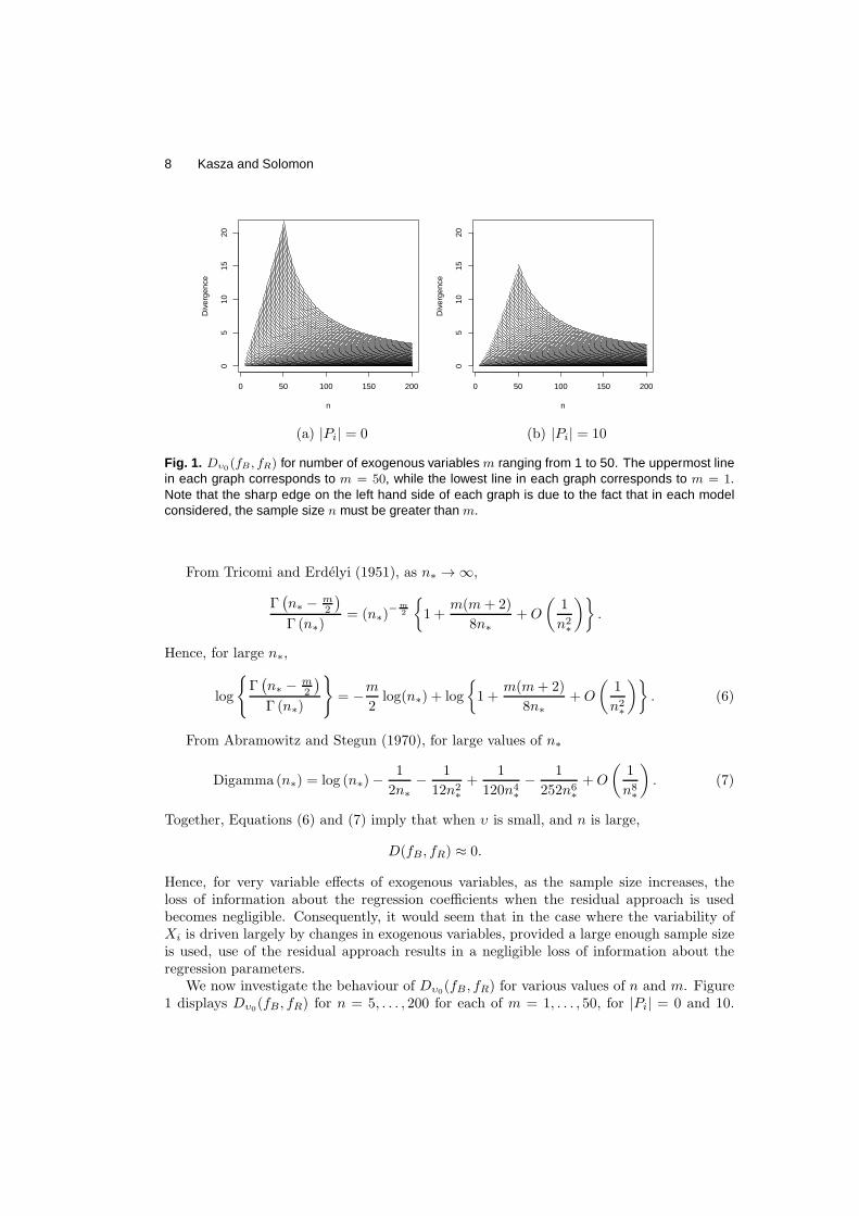
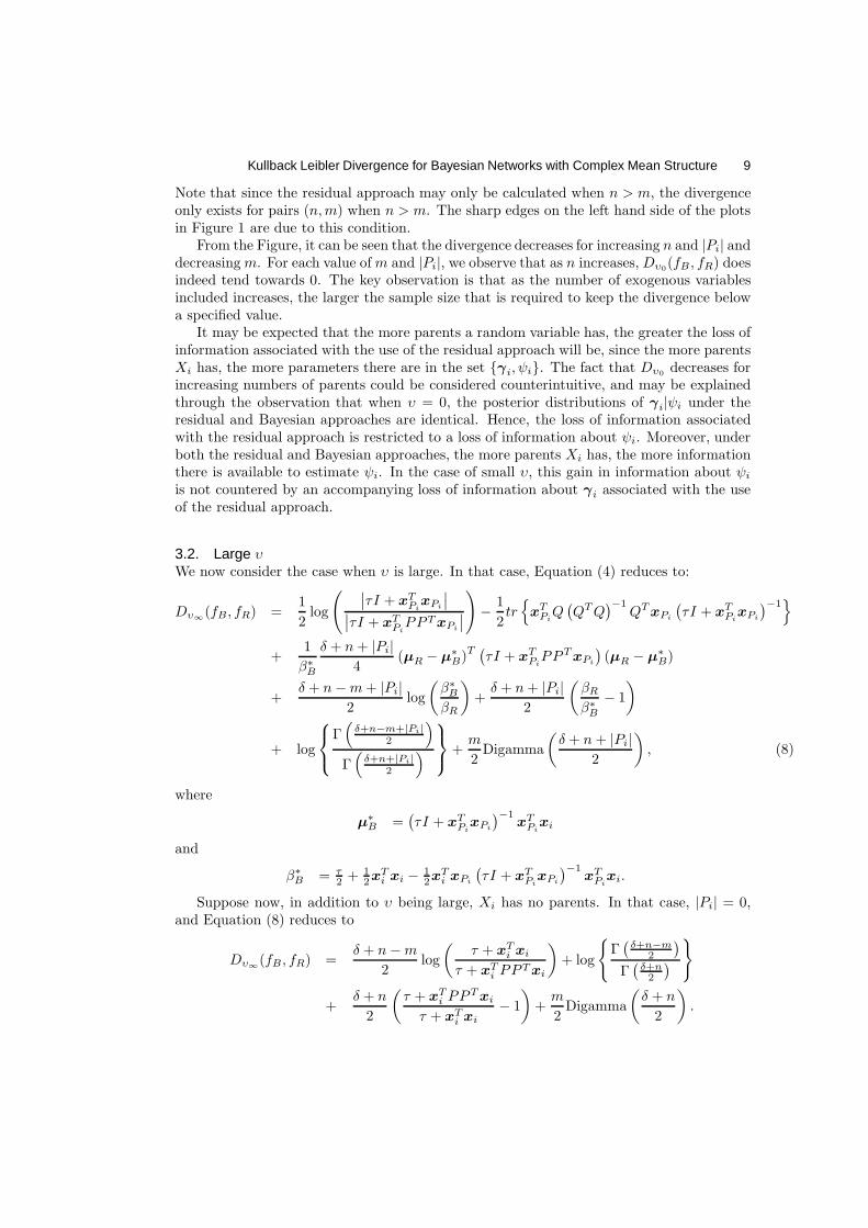
Fig. 1. Dυ0(fB , fR) for number of exogenous variables m ranging from 1 to 50. The uppermost line

in each graph corresponds to m = 50, while the lowest line in each graph corresponds to m = 1.Note that the sharp edge on the left hand side of each graph is due to the fact that in each modelconsidered, the sample size n must be greater than m.

From Tricomi and Erdelyi (1951), as n∗ → ∞,

Γ(

n∗ −m2

)

Γ (n∗)= (n∗)

−m

2

{

1 +m(m+ 2)

8n∗+O

(

1

n2∗

)}

.

Hence, for large n∗,

log

{

Γ(

n∗ −m2

)

Γ (n∗)

}

= −m

2log(n∗) + log

{

1 +m(m+ 2)

8n∗+O

(

1

n2∗

)}

. (6)

From Abramowitz and Stegun (1970), for large values of n∗

Digamma (n∗) = log (n∗)−1

2n∗−

1

12n2∗

+1

120n4∗

−1

252n6∗

+O

(

1

n8∗

)

. (7)

Together, Equations (6) and (7) imply that when υ is small, and n is large,

D(fB, fR) ≈ 0.

Hence, for very variable effects of exogenous variables, as the sample size increases, theloss of information about the regression coefficients when the residual approach is usedbecomes negligible. Consequently, it would seem that in the case where the variability ofXi is driven largely by changes in exogenous variables, provided a large enough sample sizeis used, use of the residual approach results in a negligible loss of information about theregression parameters.

We now investigate the behaviour of Dυ0(fB, fR) for various values of n and m. Figure

1 displays Dυ0(fB, fR) for n = 5, . . . , 200 for each of m = 1, . . . , 50, for |Pi| = 0 and 10.


Note that since the residual approach may only be calculated when n > m, the divergenceonly exists for pairs (n,m) when n > m. The sharp edges on the left hand side of the plotsin Figure 1 are due to this condition.

From the Figure, it can be seen that the divergence decreases for increasing n and |Pi| anddecreasingm. For each value ofm and |Pi|, we observe that as n increases,Dυ0

(fB , fR) doesindeed tend towards 0. The key observation is that as the number of exogenous variablesincluded increases, the larger the sample size that is required to keep the divergence belowa specified value.

It may be expected that the more parents a random variable has, the greater the loss ofinformation associated with the use of the residual approach will be, since the more parentsXi has, the more parameters there are in the set {γi, ψi}. The fact that Dυ0

decreases forincreasing numbers of parents could be considered counterintuitive, and may be explainedthrough the observation that when υ = 0, the posterior distributions of γi|ψi under theresidual and Bayesian approaches are identical. Hence, the loss of information associatedwith the residual approach is restricted to a loss of information about ψi. Moreover, underboth the residual and Bayesian approaches, the more parents Xi has, the more informationthere is available to estimate ψi. In the case of small υ, this gain in information about ψi

is not countered by an accompanying loss of information about γi associated with the useof the residual approach.

3.2. Large υWe now consider the case when υ is large. In that case, Equation (4) reduces to:

Dυ∞(fB, fR) =1

2log

(∣

∣τI + xTPixPi

∣

∣

∣

∣τI + xTPiPPTxPi

∣

∣

)

−1

2tr{

xTPiQ(

QTQ)−1

QTxPi

(

τI + xTPixPi

)−1}

+1

β∗B

δ + n+ |Pi|

4(µR − µ∗

B)T (

τI + xTPiPPTxPi

)

(µR − µ∗B)

+δ + n−m+ |Pi|

2log

(

β∗B

βR

)

+δ + n+ |Pi|

2

(

βRβ∗B

− 1

)

+ log

Γ(

δ+n−m+|Pi|2

)

Γ(

δ+n+|Pi|2

)

+m

2Digamma

(

δ + n+ |Pi|

2

)

, (8)

where

µ∗B =

(

τI + xTPixPi

)−1xTPixi

and

β∗B = τ

2+ 1

2xTi xi −

1

2xTi xPi

(

τI + xTPixPi

)−1xTPixi.

Suppose now, in addition to υ being large, Xi has no parents. In that case, |Pi| = 0,and Equation (8) reduces to

Dυ∞(fB, fR) =δ + n−m

2log

(

τ + xTi xi

τ + xTi PP

Txi

)

+ log

{

Γ(

δ+n−m2

)

Γ(

δ+n2

)

}

+δ + n

2

(

τ + xTi PP

Txi

τ + xTi xi

− 1

)

+m

2Digamma

(

δ + n

2

)

.

10 Kasza and Solomon

Which may be written as

Dυ∞(fB, fR) = −

(

δ + n−m

2

)

log

(

1−xTi Q

(

QTQ)−1

QTxi

τ + xTi xi

)

+ log

{

Γ(

δ+n−m2

)

Γ(

δ+n2

)

}

−δ + n

2

(

xTi Q

(

QTQ)−1

QTxi

τ + xTi xi

)

+m

2Digamma

(

δ + n

2

)

.

Sincex

T

iQ(QTQ)−1

QTxi

τ+xT

ixi

< 1,

− log

(

1−xTi Q

(

QTQ)−1

QTxi

τ + xTi xi

)

=

∞∑

k=1

1

k

(

xTi Q

(

QTQ)−1

QTxi

τ + xTi xi

)k

. (9)

Note that sincex

T

iQ(QTQ)−1

QTxi

τ+xT

ixi

< 1, higher-order terms in the sum in Equation (9)

can be safely ignored to give

Dυ∞(fB, fR) = −δ + n

2

(

xTi Q

(

QTQ)−1

QTxi

τ + xTi xi

)

+δ + n−m

2

(

xTi Q

(

QTQ)−1

QTxi

τ + xTi xi

)

+ log

{

Γ(

δ+n−m2

)

Γ(

δ+n2

)

}

+m

2Digamma

(

δ + n

2

)

.

If the data are centred and scaled:

Dυ∞(fB, fR) = −δ + n

2

(

xTi Q

(

QTQ)−1

QTxi

τ + n− 1

)

+δ + n−m

2

(

xTi Q

(

QTQ)−1

QTxi

τ + n− 1

)

+ log

{

Γ(

δ+n−m2

)

Γ(

δ+n2

)

}

+m

2Digamma

(

δ + n

2

)

.

Note that xTi Q

(

QTQ)−1

QTxi ≤ n− 1, so

Dυ∞(fB, fR) ≤ −δ + n

2

(

n− 1

τ + n− 1

)

+δ + n−m

2

(

n− 1

τ + n− 1

)

+ log

{

Γ(

δ+n−m2

)

Γ(

δ+n2

)

}

+m

2Digamma

(

δ + n

2

)

.

It can then be seen that as n increases, terms cancel, and D(fB, fR) approaches 0.

We now consider Dυ∞ for |Pi| ≥ 1. First, note that

log

(∣

∣τI + xTPixPi

∣

∣

∣

∣τI + xTPiPPTxPi

∣

∣

)

= − log{∣

∣

∣I − xTPiQ(

QTQ)−1

QTxPi

(

τI + xTPixPi

)−1∣

∣

∣

}

.


For a square matrix X , |X | = exp {tr [log(X)]}, so that

log(∣

∣

∣I − xTPiQ(

QTQ)−1

QTxPi

(

τI + xTPixPi

)−1∣

∣

∣

)

= tr[

log{

I − xTPiQ(

QTQ)−1

QTxPi

(

τI + xTPixPi

)−1}]

= tr

[

−

∞∑

k=1

1

k

{

xTPiQ(

QTQ)−1

QTxPi

(

τI + xTPixPi

)−1}k

]

= −

∞∑

k=1

1

ktr

[

{

xTPiQ(

QTQ)−1

QTxPi

(

τI + xTPixPi

)−1}k]

.

Additionally,

δ + n−m+ |Pi|

2log

(

β∗B

βR

)

=δ + n−m+ |Pi|

2

∞∑

k=1

1

k

(

β∗B − βRβ∗B

)k

,

so that the divergence in Equation (8) becomes

Dυ∞(fB, fR) =1

2

∞∑

k=2

1

ktr

[

{

xTPiQ(

QTQ)−1

QTxPi

(

τI + xTPixPi

)−1}k]

+1

β∗B

δ + n+ |Pi|

4(µR − µ∗

B)T (τI + xT

PiPPTxPi

)

(µR − µ∗B)

−

(

δ + n+ |Pi|

2

)(


)

+δ + n−m+ |Pi|

2

∞∑

k=1

1

k

(


)k

+ log

Γ(

δ+n−m+|Pi|2

)

Γ(

δ+n+|Pi|2

)

+m

2Digamma

(

δ + n+ |Pi|

2

)

.

Sinceβ∗B−βR

β∗B

< 1, second- and higher-order terms in∑∞

k=11

k

(

β∗B−βR

β∗B

)k

may safely be

ignored, as they were in the derivation of D(fB, fR) for large υ in the case of no parents,to give

Dυ∞(fB, fR) ≈1

2

∞∑

k=2

1

ktr

[

{

xTPiQ(

QTQ)−1

QTxPi

(

τI + xTPixPi

)−1}k]

+1

β∗B

δ + n+ |Pi|

4(µR − µ∗

B)T (

τI + xTPiPPTxPi

)

(µR − µ∗B)

−

(

δ + n+ |Pi|

2

)(


)

+δ + n−m+ |Pi|

2

(


)

+ log

Γ(

δ+n−m+|Pi|2

)

Γ(

δ+n+|Pi|2

)

+m

2Digamma

(

δ + n+ |Pi|

2

)

.

In considering the trace term, note that xTPiQ(

QTQ)−1

QTxPiand

(

τI + xTPixPi

)−1are


both positive semi-definite matrices, so that

tr

[

{

xTPiQ(

QTQ)−1

QTxPi

(

τI + xTPixPi

)−1}k]

≤ tr{

xTPiQ(

QTQ)−1

QTxPi

(

τI + xTPixPi

)−1}k

≤[

tr{

xTPiQ(

QTQ)−1

QTxPi

}

tr{

(

τI + xTPixPi

)−1}]k

=

tr{

(

τI + xTPixPi

)−1}

∑

j∈Pi

xTj Q

(

QTQ)−1

QTxj

k

Approximating(

τI + xTPixPi

)−1by diag(τ + xT

k xk) gives

∑

j∈Pi

1

τ + xTj xj

∑

j∈Pi

xTj Q

(

QTQ)−1

QTxj

k

,

which, if data are centered and scaled, becomes

|Pi|∑

j∈Pi

xTj Q

(

QTQ)−1

QTxj

τ + n− 1

k

.

Hence, as n gets large, the trace term in Dυ∞ will approach zero.We now consider the quadratic term

1

β∗B

δ + n+ |Pi|

4(µR − µ∗

B)T (

τI + xTPiPPTxPi

)

(µR − µ∗B)

Using the following approximations,

(

τ + xTPixPi

)−1≈ diag

(

1

τ + xTk xk

)

,

(

τ + xTPiPPTxPi

)−1≈ diag

(

1

τ + xTk xk − xT

kQ(QTQ)−1QTxk

)

where k ∈ Pi, we may write

β∗B ≈

τ

2+

xTi xi

2−

1

2

∑

k∈Pi

(xTi xk)

2

τ + xTk xk

and

(µR − µ∗B)

T (

τI + xTPiPPTxPi

)

(µR − µ∗B)

=∑

k∈Pi

{

(

xiPPTxk

)2

τ + xTk xk − xT

kQ (QTQ)−1QTxk

}

− 2∑

k∈Pi

(

xTi xkxiPP

Txk

τ + xTk xk

)

+∑

k∈Pi

(xTi xk)

2

(

τ + xTk xk − xT

kQ(

QTQ)−1

QTxk

)

(τ + xTk xk)2

. (10)


As n increases, δ+n+|Pi|β∗B

approaches 1, and each of the terms in Equation (10) approacheszero.

It is thus clear that as n approaches infinity, Dυ∞ approaches zero.

3.3. Behaviour of D as n→ ∞Given the machinery in the above proofs that Dυ0

and Dυ∞ approach zero as n approachesinfinity, it is not difficult to show that D approaches zero as n→ ∞ for all values of υ.

First, consider the log determinant term of D:

1

2log

(∣

∣τI + xTPiHυxPi

∣

∣

∣

∣τI + xTPiPPTxPi

∣

∣

)

= −1

2log{∣

∣

∣

(

τI + xTPiHυxPi

)−1 (

τI + xTPiPPTxPi

)

∣

∣

∣

}

= −1

2tr[

log{

(

τI + xTPiHυxPi

)−1 (

τI + xTPiPPTxPi

)

}]

= −1

2tr(

log[

I −{

I −(

τI + xTPiHυxPi

)−1 (

τI + xTPiPPTxPi

)

}])

,

using the Taylor series expansion,

= −1

2tr

[

−∞∑

k=1

1

k

{

I −(

τI + xTPiHυxPi

)−1 (

τI + xTPiPPTxPi

)

}k

]

.

If second- and higher-order terms are ignored, this becomes

1

2tr{

I −(

τI + xTPiHυxPi

)−1 (

τI + xTPiPPTxPi

)

}

=|Pi|

2−

1

2tr{

(

τI + xTPiHυxPi

)−1 (

τI + xTPiPPTxPi

)

}

,

terms which cancel with other terms in D.Consider now the quadratic term:

1

βB

δ + n+ |Pi|

4(µR − µB)

T (τI + xTPiPPTxPi

)

(µR − µB) .

Using approximations similar to those used for the analogous term in Dυ∞ , it can be shownthat as n approaches ∞, this quadratic term approaches zero.

The remaining terms in D can be shown to approach zero using arguments similar tothose used for Dυ0

and Dυ∞ . Hence, as n→ ∞, D → 0.

3.4. Loss of Information about the Joint Marginal Covariance MatrixThe loss of information about the parameters associated with each of the marginal regressionmodels may be combined to give the total loss of information about the marginal covariancematrix ofX, denoted by Σ, when the residual approach, rather than the Bayesian approach,is used. If the underlying graphical structure of X is known, this quantity may be writtenas

DΣ {fB(Σ|X), fR(Σ|X)} =

p∑

i=1

D {fB(γi, ψi|xi,xPi), fR(γi, ψi|xi,xPi

)} .


Of course, in general, the underlying dependence structure of X is unknown, and is esti-mated using either the Bayesian or residual score metric in conjunction with a score-basedapproach for the estimation of Bayesian networks. If the structure is unknown, the exactamount of information lost about the covariance matrix cannot be calculated. However,some information about the amount of information lost through the use of the residualapproach can be obtained. By considering the divergence for the covariance matrix corre-sponding to the graph with no edges:

DeΣ =

p∑

i=1

D {fB(γi, ψi|xi), fR(γi, ψi|xi)} ,

and the divergence for the covariance matrix of an arbitrary full graph:

DfΣ=

p∑

i=1

D {fB(γi, ψi|xi,x1, . . . ,xi−1), fR(γi, ψi|xi,x1, . . . ,xi−1)}

one can get an idea of how much information will be lost about the covariance matrix of anarbitrary graph.

For small values of υ,

DfΣ≤ DΣ {fB(Σ|X), fR(Σ|X)} ≤ De

Σ.

For large values of υ, the inequalities must be reversed.These bounds arise from the fact that for small values of υ, the fewer parents each Xi

has, the greater the amount of information that will be lost when the residual approachis used. Hence, the amount of information lost will be maximised for the directed acyclicgraph without any edges, and minimised for a complete graph. For large values of υ, thefewer parents each Xi has, the less the amount of information that will be lost through theuse of the residual approach, leading to the reversal of the above bounds. Note that thedefinitions of “small υ” and “large υ” are data dependent. We shed some light on this issuethrough examination of some examples in Section 4.

The reversal of bounds indicates that there exists a value of υ such that

DfΣ= De

Σ.

Hence, the divergence of a given graph will not lie between DfΣ

and DeΣ for all values of

υ: there will exist “intermediate” values of υ such that DΣ {fB(Σ|X), fR(Σ|X)} is not

bounded by DfΣand De

Σ. However, for all graphical structures, DΣ {fB(Σ|X), fR(Σ|X)}

will always be bounded by the maximum of Deυ0,Σ

and Dfυ∞,Σ, where

Deυ0,Σ

=

p∑

i=1

Dυ0{fB(γi, ψi|xi), fR(γi, ψi|xi)} ,

Dfυ∞,Σ =

p∑

i=1

Dυ∞ {fB(γi, ψi|xi,x1, . . . ,xi−1), fR(γi, ψi|xi,x1, . . . ,xi−1)} .

4. Examples

In this section, we examine the loss of information associated with the residual approachfor some specific data sets. We first consider data simulated from a known structure. We


1

2

3 4 5

6

7 8 9 10

Fig. 2. Connected components of the underlying graph of Example 1.

then consider a data set consisting of expression levels of grape heat-shock genes, where thegrapes were sampled from 3 different vineyards, and air temperatures in the hours leadingup to the picking of the grapes was recorded.

4.1. Example 1In this example, multiple data sets were simulated from the following system of linearrecursive equations:

Xijk =

i−1∑

l=1

γi,lXljk + bij + ǫijk,

ǫijk ∼ N(0, ψi),

bij ∼ N(0, ψi/υ)

γi,l ∼ N(0, ψi)

ψi ∼ Inverse Gamma(1, 2)

i = 1, . . . , 20, j = 1, 2, k = 1, . . . , n,

where the only non-zero γi,ls were those corresponding to the edges in the graph of Figure2. One hundred data sets were simulated according to this model for each pair (n, υ), wheren = 5, 10, 20, 50, 100 and υ = 0.001, 0.01, 0.1, 1, 10, 100. Note that when υ = 1, γi and biare independent and identically distributed; for υ < 1, the bi are more variable than theγi; and for υ > 1, the bi are less variable than the γi.

For each of the simulated data sets, DfΣ, De

Σ, and the divergence corresponding to thetrue structure were calculated. The results displayed in Figure 3 show, for the 100 simulateddata sets corresponding to each (n, υ) pair, the median value of the divergence for each ofthe three structures considered, and the upper and lower quartiles.

Due to the level of sparsity in the true graph, the divergence associated with this graphis, particularly for smaller sample sizes, closer to that of the empty graph than that of thefull graph. As expected, for all values of υ, as sample size increases, divergence decreases.For small values of υ, the divergence corresponding to the true graph is less than thatcorresponding to the empty graph, while for larger values of υ, the opposite is true, the

16 Kasza and Solomon0

24

6

upsilon=0.001

Sample size

Div

erge

nce

5 10 20 50 100

01

23

45

67

upsilon=0.01

Sample size

Div

erge

nce

5 10 20 50 100

02

46

810

upsilon=0.1

Sample size

Div

erge

nce

5 10 20 50 100

010

2030

upsilon=1

Sample size

Div

erge

nce

5 10 20 50 100

010

3050

upsilon=10

Sample size

Div

erge

nce

5 10 20 50 100

010

3050

upsilon=100

Sample size

Div

erge

nce

5 10 20 50 100

Fig. 3. The results of Example 1. The open circles represent the median value of DeΣ, the filled

circles the median value of Df

Σ, and the triangles the median loss associated with the true structure,

of the 100 simulated data sets for each (n, υ) pair. The vertical bars represent interquartile ranges.Note that the vertical scales of the plots differ.

cause of which was discussed in Section 3.4. This result can be seen to depend, not only onthe size of υ, but also on sample size.

Note also that, for all sample sizes, but particularly for n = 5, 10 or 25, as υ increases,a general increase in divergence can be seen. This is due to the fact that when υ is large,the variance of the effects of exogenous variables is small, and the samples that makeup the data set being considered are “similar” to independent and identically distributedsamples. By taking the Hυ matrix to be close to an identity matrix, the Bayesian approachallows for this, performing in a manner similar to when the data set does indeed consist ofindependent and identically distributed samples. Of course, the residual approach cannotadjust for this, as the PPT matrix is the same no matter what the variance of the effectsof the exogenous variables is. Hence, the exogenous variables are over-corrected for whenthe residual approach is taken, and an additional loss of information results.

For n = 50 or 100, the values of the divergences for the three graphs considered arerelatively small for all values of υ, indicating that little information about the marginalcovariance matrix is lost through the use of the residual approach. In addition, for theselarger sample sizes, divergences for the covariance matrices corresponding to the full andempty graphs do not differ by a large amount, and the figure shows that these quantitiesprovide reasonable approximations for the divergence associated with the true structure.

These observations are particularly important when it comes to providing guidelines forthe use of the residual approach in the estimation of a Bayesian network for a given data set.On the basis of this example, it seems that if υ is small, no matter what the size of the ration/p is, the amount of information about the marginal covariance matrix lost through theuse of the residual approach will be negligible. In the case where n/p is small, provided υ islarge, a similar conclusion is reached, that is, the amount of information lost will again be


small. However, for data sets with small values of n/p, if the effect of exogenous variablesare a priori thought to have small variances, the residual approach must be used withcaution, as the loss of information associated with this approach could be large.

For all data sets, before the residual approach is used, it is recommended that DeΣ and

DfΣbe calculated to provide bounds on the amount of information lost about the marginal

covariance matrix when the residual approach is used. If the calculated values of DeΣ and

DfΣare large, caution is required in the use of the residual approach. In the next example,

we calculate DeΣ and Df

Σfor a data set consisting of gene expression levels, where neither

the true structure nor the true value of υ are known.

4.2. Grape gene exampleWe now consider a data set consisting of samples of the expression levels of grape genes;an example previously discussed in Kasza et al. (2010). This data set consists of n = 50expression levels of each of p = 26 grape genes, where the grapes themselves were sampledfrom 3 different vineyards located in different wine growing regions of South Australia.These 26 genes are heat-shock genes, see Wang et al. (2004), the expression levels of whichare known to be associated with changes in temperature. Accordingly, air temperatureat each vineyard was recorded every hour from 5.5 hours to 0.5 hours before grapes weresampled.

The data set considered here is actually a subset of a larger data set obtained from anAffeymetrix chip microarray experiment conducted over the course of three years. Geneexpression values were obtained from 174 grape berry tissue samples; 68 of these tissuesamples were taken from one vineyard, 68 from the second vineyard, and 38 from the third.At the first two vineyards, four grape berry tissue samples were selected each week for17 weeks, while at the third, 2 grape berry tissue samples were selected each week for 19weeks. At each of the vineyards, the first samples were taken at fruit set, when the fertilisedgrape flowers began to form berries. Samples were then taken each week for a pre-specifiednumber of weeks. In this way, gene expression levels were measured over the course of thedevelopment of the grape berries. Of the 174 samples taken, a total of 162 had completetemperature records.

The reduced data set considered here, consisting of 50 expression levels for each gene,consists of the samples from each vineyard taken in the third to seventh weeks of sampling,inclusive. The reason for the use of these samples is that the samples from these weekscorrespond to a period after fruit set, but before veraison, see Coombe (1973) and Robinsonand Davies (2000) for details. It is thought that the relationships between expression levelsof genes are quite stable during this period of berry development.

Let Xij be sample j of gene i, i = 1, . . . , 26, j = 1, . . . , 50, and let qrj be the dataassociated with sample j of exogenous variable r, where m exogenous variables are includedin the model. Then the following model is assumed for each sample of each gene:

Xij =∑

l∈Pi

γilXlj +

m∑

r=1

qrjbir + ǫij , ǫij ∼ N(0, ψi),

γil ∼ N(0, τ−1ψi),

ψi ∼ Inverse Gamma

(

δ + |Pi|

2,τ

2

)

,

bir ∼ N(0, υ−1ψi). (11)


For this example, as is the case with most real-world examples, the true form of theeffects of the exogenous variables on expression levels is unknown, and difficult to determine.Additionally, estimates of these effects are of little interest in this example, which areincluded primarily to improve the estimation of the joint dependence structure of the genes.For these reasons, the use of the residual approach in the analysis of this data set wasadvocated in Kasza (2009). Here the loss of information associated with this approach,assuming that the true distribution of each bir is as given in Equation (11), is furtherinvestigated.

It is not completely clear which set of variables should be included in the model asexogenous variables in this example. For the grape genes considered here, temperature,which has been directly observed at the different vineyards, is a known driver of biologicalactivity. When two or more genes respond similarly to the same driver of biological activity,the effect is to produce a component of correlation between the corresponding expressionlevels. There are also likely to be additional covariates which do not correspond directlyto a single biological factor such as temperature. For example, the three vineyards arelikely to differ in a number of features such as soil type and fertility, moisture and othermicro-climate conditions, each of which could potentially influence the expression levels ofcertain sets of genes. Here the three vineyards are separated by large regional distances,but share the same macro-climate in South Australia.

Hence, to a large extent, changes in temperature and vineyard are confounded, andshould not be included together in a Bayesian network model which aims to interpret theresidual (biological) correlation structure, even when potential interactions of temperatureand vineyard may be of interest. To include both temperature and vineyard effects inthe analysis of this data set would be to risk over-parameterising the model, and thereforeover-fitting the data, resulting in the removal of dependencies of plausible biological interest.Hence, the consideration of models including both vineyard and temperature effects will nothelp shed light on the performance of the residual approach to the estimation of Bayesiannetworks.

Thus, here we consider the vineyards only model, where m = 3 and in which we areinterested in the temperature-induced correlations between genes, and the temperatureonly model, where m = 6, where we do not remove directly the components of correlationsinduced by the vineyard micro-climates, which may also be of substantive interest. Notethat we are ignoring the temperature trend component in all our models. Although modelscontaining both temperature and vineyard effects may potentially be of interest, the effectsmay be confounded as explained above, and there is a risk of over-fitting the data. In fact,for the full interaction model fitted to the grape gene data, the effective sample size, n−m,would be effectively zero, and the Kullback Leibler divergence could be inflated.

Since neither the true network nor the true value of υ are known for this data set, thebounds De

Σ and DfΣare calculated for a range of values of υ, for the two considered sets of

exogenous variables. The results are displayed in Figure 4. The left graph in that figuredisplays the loss of information when the three vineyard effects are included in the analysisonly and the right graph displays the divergence when only the six main temperature effectsare included. At first glance, it may appear that the behaviours of De

Σ and DfΣare different

in the two graphs, but this perceived difference is due only to the range of values of υconsidered. If the divergences were calculated for larger values of υ, it would be seen thatthe divergences do have a similar shape for both of the models considered. However, weconsider the range of values of υ here to be sufficient.

The figure indicates that, for either of the two considered models, and for all considered


0 2 4 6 8 10

05

1015

20Vineyards

upsilon

Div

erge

nce

0 2 4 6 8 10

05

1015

20

Temperatures

upsilon

Div

erge

nce

Fig. 4. Upper and lower bounds of the divergence for the marginal covariance matrix of the 26 grapegenes, when vineyards and then temperatures are included as exogenous variables in the analysis.In both graphs, the solid line is the divergence corresponding to the empty graph, and the dashedline is the divergence corresponding to the full graph.

values of υ, if the true underlying graph is thought to be sparse, as many biological networksare thought to be, the loss of information about the marginal covariance matrix when theresidual approach is used will be minimal. If the true graph of the expression levels of theconsidered genes is thought to be dense, for larger values of υ, the figure shows that theloss of information for the temperature model will be less than that associated with thevineyard model. The temperature model is likely to be more explanatory, with a highernumber of exogenous variables fitted. For either model, the Kullback Leibler divergence issmall and the residual approach to estimation is of practical utility.

5. Conclusion

In this paper, we have compared two methods for estimating Bayesian networks for datacontaining exogenous variables. Provided that sample size is not too small in a statisticalsense, we can conclude that the residual score estimation approach offers a useful alternativeto a fully Bayesian approach, with generally negligible loss of information about key pa-rameters and features of interest. Many contemporary bioinformatics and genomics studiesare designed and conducted using substantial sample sizes, often based on many hundredsof samples or patients. Not all studies will be this large, as is the case for our grape geneexample in Section 4, but the results of our simulation studies provide confidence that theresidual estimation approach performs well with small samples in the presence of exogenousvariables.


Acknowledgments

Jessica Kasza thanks the ECMS Faculty Research Scheme, University of Adelaide, for fi-nancial support for her visit to Patty Solomon, during which this work was begun.

Appendix AIn this appendix, some details on the derivation of the Kullback Leibler divergence given inEquation (4) are provided. Equation (4) may be written as

D(fB, fR) =

∫

R|Pi|

∫ ∞

0

fB (γi, ψi|xi,xPi) log

{

fB (γi, ψi|xi,xPi)

fR (γi, ψi|xi,xPi)

}

dψidγi

=

∫

R|Pi|

∫ ∞

0

fB (γi|xi,xPi, ψi) fB (ψi|xi,xPi

) log

{

fB (γi|xi,xPi, ψi)

fR (γi|xi,xPi, ψi)

}

dψidγi

+

∫

R|Pi|

∫ ∞

0

fB (γi|xi,xPi, ψi) fB (ψi|xi,xPi

) log

{

fB (ψi|xi,xPi)

fR (ψi|xi,xPi)

}

dψidγi

=

∫ ∞

0

fB (ψi|xi,xPi)

∫

R|Pi|

fB (γi|xi,xPi, ψi) log

{



}

dγidψ

+

∫ ∞

0

fB (ψi|xi,xPi) log

{

fB (ψi|xi,xPi)

fR (ψi|xi,xPi)

}

dψi. (12)

Note that∫

R|Pi|


{



}

dγi

is the Kullback Leibler divergence of two multivariate normal distributions. Hence,∫

R|Pi|


{



}

dγi

=1

2log

(∣

∣τI + xTPiHυxPi

∣

∣

∣

∣τI + xTPiPPTxPi

∣

∣

)

+1

2tr{

(

τI + xTPiPPTxPi

) (

τI + xTPiHυxPi

)−1}

−|Pi|

2+

1

2ψi

(µR − µB)T (

τI + xTPiPPTxPi

)

(µR − µB) ,

so the first component of Equation (12) is given by

1

2log

(∣

∣τI + xTPiHυxPi

∣

∣

∣

∣τI + xTPiPPTxPi

∣

∣

)

+1

2tr{

(

τI + xTPiPPTxPi

) (

τI + xTPiHυxPi

)−1}

−|Pi|

2+

1

βB

δ + n+ |Pi|

4(µR − µB)

T (

τI + xTPiPPTxPi

)

(µR − µB) . (13)

To find the second component of Equation (12), note that

log

{

fB (ψi|xi,xPi)

fR (ψi|xi,xPi)

}

=δ + n+ |Pi|

2log(βB)−

(

δ + n−m+ |Pi|

2

)

log(βR)

+ log

Γ(

δ+n−m+|Pi|2

)

Γ(

δ+n+|Pi|2

)

−m

2log(ψi) + (βR − βB)

1

ψi

.


Hence,

∫ ∞

0

fB (ψi|xi,xPi) log

{

fB (ψi|xi,xPi)

fR (ψi|xi,xPi)

}

dψi

=δ + n+ |Pi|

2log(βB)−

δ + n−m+ |Pi|

2log(βR) + log

Γ(

δ+n−m+|Pi|2

)

Γ(

δ+n+|Pi|2

)

+δ + n+ |Pi|

2

(

βRβB

− 1

)

−m

2

{

log(βB)−Digamma

(

δ + n+ |Pi|

2

)}

=δ + n−m+ |Pi|

2log

(

βBβR

)

+ log

Γ(

δ+n−m+|Pi|2

)

Γ(

δ+n+|Pi|2

)

+δ + n+ |Pi|

2

(

βRβB

− 1

)

+m

2Digamma

(

δ + n+ |Pi|

2

)

. (14)

Adding together Equations (13) and (14) then gives the Kullback Leibler divergence shownin Equation (4).

References

Abramowitz, M. and Stegun, I. A., editors. (1970) Handbook of Mathematical Functions

with Formulas, Graphs, and Mathematical Tables. Washington, D. C.: National Bureauof Standards.

Cooper, G. F. and Herskovits, E. (1992) A Bayesian method for the induction of proba-bilistic networks from data. Machine Learning, 9, 309-347.

Coombe, B. G. (1973) The regulation of set and development of the grape berry. Acta

Horticulturae, 34, 261-271.

Dobra, A., Hans, C., Jones, B., Nevins, J.R. and West, M.(2004) Sparse graphical modelsfor exploring gene expression data. Journal of Multivariate Analysis, 90, 196-212.

Geiger, D. and Heckerman, D. (1994) Learning Gaussian networks. In Proceedings of the

Tenth Conference on Uncertainty in Artificial Intelligence.

Geiger, D. and Heckerman, D. (2002) Parameter priors for directed acyclic graphical modelsand the characterization of several probability distributions. The Annals of Statistics, 30,1412-1440.

Kasza, J. (2009) Bayesian networks for high-dimensional data with complex mean structure.Ph. D. thesis, The University of Adelaide.

Kasza, J. E., Glonek, G. and Solomon, P. (2010) Estimating Bayesian networks for high-dimensional data with complex mean structure. arXiv:1002.2168.

Kullback, S. and Leibler, R. A. (1951) On information and sufficiency. The Annals of

Mathematical Statistics, 22, 79-86.

Lauritzen, S. L. (2004) Graphical Models. Oxford: Clarendon Press.


Robinson, S. P. and Davies, C. (2000) Molecular biology of grape berry ripening. AustralianJournal of Grape and Wine Research, 6, 175-188.

Sachs, K., Perez, O., Pe’er, D., Lauffenburger, D. A. and Nolan, G. P. (2005) Causalprotein-signaling networks derived from multiparameter single-cell data. Science, 308,523-529.

Tricomi, F. G. and Erdelyi, A. (1951) The asymptotic expansion of a ratio of gammafunctions. Pacific Journal of Mathematics, 1, 133-142.

Wang, W., Vinocur, B., Shoseyov, O. and Altman, A. (2004) Role of plant heat-shockproteins and molecular chaperones in the abiotic stress response. Trends in Plant Science,9, 244-252.

Kullback Leibler Divergence forBayesian Networks with Complex … · 2 Kasza and Solomon for the...

Documents

Transcript of Kullback Leibler Divergence forBayesian Networks with Complex … · 2 Kasza and Solomon for the...