KREPS CH 17ADVERSE SELECTION & MARKET SIGNALING 1INTRODUCTIONINTRODUCTION Greshman’s Law...

KREPS CH 17 ADVERSE SELECTION & MARKET SIGNALING

1

INTRODUCTION INTRODUCTION INTRODUCTION INTRODUCTION

Greshman’s LawGreshman’s Law ; bad money derives out good money .

The holder of a coin is able to shave a bit of gold from it in a way that is undetectable without careful measurement ; the gold so obtained can then be used to produce new coins .

The holder of an unshaved coin will therefore withhold the coin from trade ; only the shaved coins will circulate.


2

AKERLOF’S MODEL OF LEMONSAKERLOF’S MODEL OF LEMONS

Bad used cars derives out good cars out of market .Bad used cars derives out good cars out of market .

suppose that there are two types of used care ; peaches and lemonspeaches and lemons

1- a peach worth $3000 to a buyer & $2500 to a seller . The supply of peach cars is fixed and the demand of possible buyers are infinite , so that the equilibrium price in equilibrium price in the peach market is $3000 . the peach market is $3000 .

2- a lemon worth $2000 to a buyer and $1000 to a seller . There are twice as many twice as many lemons as peaches .lemons as peaches .

We can summarize the worth of different kinds in the following table ,

lemons peacheslemons peaches

Sellers 1000 2500Sellers 1000 2500

Buyers 2000 3000Buyers 2000 3000

Different kinds of transaction could be recognized ;


3


1- if buyers and sellers both had the ability to look at the car and 1- if buyers and sellers both had the ability to look at the car and recognize the type of the carrecognize the type of the car , peaches will be sold for $3000 and lemons will be sold for $2000.

2- if neither buyer nor seller knew whether a particular car was a peach if neither buyer nor seller knew whether a particular car was a peach or lemon and assuming risk neutrality we would have no problem .or lemon and assuming risk neutrality we would have no problem .

a- a- a seller thinkinga seller thinking that she has a peachespeaches with probability of 1/3probability of 1/3 and a lemon lemon with the probability of 2/3 .2/3 .

She also expect that she might have a car with the expected value expected value

equal to $1500 = (1/3)(2500) + (2/3) (1000)equal to $1500 = (1/3)(2500) + (2/3) (1000)

b-b- a buyer assuminga buyer assuming the same probability the same probability expect that she might buy a car with expected value equal to 2333.3 = (1/3)(3000) + (2/3)(2000)2333.3 = (1/3)(3000) + (2/3)(2000)

Assuming inelastic supply and elastic demand the market clears at a Assuming inelastic supply and elastic demand the market clears at a price equal to $2333.3 price equal to $2333.3

But in reality the market is not like neither of these .


4

AKERLOF’S MODEL OF LEMONSAKERLOF’S MODEL OF LEMONSIn the market of used cars , the seller have lived with car for a while and

knows whether the car is peach or lemon . But the buyer does not have inside information about the car , expect for the quick inspection when he wants to buy it .

If we assume that the buyer’s can not tell at all , the peaches market If we assume that the buyer’s can not tell at all , the peaches market breaks downbreaks down . Suppose that cars are offered for sale at any price above Suppose that cars are offered for sale at any price above $1000 . All the lemons will appear in the market. Peaches would appear $1000 . All the lemons will appear in the market. Peaches would appear in the market at prices above $2500in the market at prices above $2500 since

lemons peaches Sellers 1000 2500 Buyers 2000 3000

At a price between $1000 and $2500At a price between $1000 and $2500 the rational buyer suppose that peaches does not appear in the marketpeaches does not appear in the market. So the cars worth only $2000 to the buyers.

At any price above $2500 , the expected value (price) of the car to the buyer At any price above $2500 , the expected value (price) of the car to the buyer is equal to 2333.3 = (1/3)(3000) + (2/3)(2000) <2500is equal to 2333.3 = (1/3)(3000) + (2/3)(2000) <2500 . There will not There will not be any offer for peaches.be any offer for peaches. Only lemons will be sold for $2000Only lemons will be sold for $2000 . (demand demand is perfectly elastic and supply is perfectly inelastic.is perfectly elastic and supply is perfectly inelastic.


5

AKERLOF’S MODEL OF LEMONSAKERLOF’S MODEL OF LEMONSSuppose that there were two peaches for every lemon . So probabilities

are as follows ;

lemons ( P = 1/3) peaches (P = 2/3 )lemons ( P = 1/3) peaches (P = 2/3 )

Sellers $ 1000 $2500

Buyers $2000 $3000

Exp (buyer) = (1/3)(2000) + (2/3)($3000) = 2666.67 > 2500

This is enough for the owners of peaches to sell and we get the market clearing price at 2666.67 with all the cars for sale . The buyer buys a car at 2666.67 and he does not know whether it is lemon or peach. Owners of peaches are not pleased about the lemons ; without them , Owners of peaches are not pleased about the lemons ; without them , peach owners would be getting an extra of 333.33=3000-2666.67 for peach owners would be getting an extra of 333.33=3000-2666.67 for their peaches . their peaches . But at least peaches can be sold .

If a particular good or service comes in many different qualities , and in a , and in a transaction one side but not the other knows the quality in advance , the transaction one side but not the other knows the quality in advance , the

other side must worry that it will get an other side must worry that it will get an adverse selectionadverse selection out of out of entire populatioentire population n . .


6

AKERLOF’S MODEL OF LEMONSAKERLOF’S MODEL OF LEMONSThe classical example of this is in life life /health insurance . If premiums are set at

fair rates for the population as a whole , insurance may be a bad deal for healthy people , who then will refuse to buy .

The problem noted above becomes worse the greater the number of qualities of cars and the smaller the valuation gap , the difference between what a car is worth to a buyer and a seller , assuming they have the same information . Note the following example ;

Imagine for example , that the quality spectrum of used cars runs from real Imagine for example , that the quality spectrum of used cars runs from real peaches , worth $2900 to sellers and $3000 to buyers , down to real lemons , peaches , worth $2900 to sellers and $3000 to buyers , down to real lemons , worth 1900 to sellers and 2000 to buyersworth 1900 to sellers and 2000 to buyers . Between the two extremes are cars Between the two extremes are cars of every quality level , always worth $100 more to buyers than sellersof every quality level , always worth $100 more to buyers than sellers . The The distribution of quality levels between these two levels are uniform . Suppose distribution of quality levels between these two levels are uniform . Suppose that there are that there are 10001 cars one of which worth $1900 to its owner and $2000 to buyers, a second worth $1900.10 to its owner and $2000.10 to buyers , and so on . Assuming inelastic supply and elastic demand at every level of quality , Assuming inelastic supply and elastic demand at every level of quality , what will be the equilibrium .what will be the equilibrium .

AKERLOF’S MODEL OF LEMONSAKERLOF’S MODEL OF LEMONSTotal number of cars = 10001 types

Each one represents a different ( quality ) kind


7

Quality of cars Worth to seller Worth to buyer Number offered

Real Peaches 2900 3000 10001

…………..

Tenth quality level better

1901 2001 11

……..………..

Second quality level better

1900.2 2000.2 3

First quality level better

1900.1 2000.1 2

Real Lemon 1900 2000 1


8

AKERLOF’S MODEL OF LEMONSAKERLOF’S MODEL OF LEMONSSupply curve would be as follows;

Min supply price for lemons to be offered = 1900 → only one car will be offered

If p = 1900.1 → 2 cars will be offered .

If p = 1900.2 → 3 cars will be offered.

If p = 1901 → 11 cars will be offered.

If p = 1902 → 21 cars will be offered.

If p = 2900 → all 10001 cars will be offered for sale.

quantity

price

2001 10001

19002100

2900

supply

demand


9


Demand curve would be perfectly elastic as follows;Demand curve would be perfectly elastic as follows;Buyers are willing to pay $2000 for real lemons and $3000 for real peaches.

Demand price will be between $2000 & $3000 .

If a car be offered at a price equal to P where 2000≤ P ≤ 3000 buyers If a car be offered at a price equal to P where 2000≤ P ≤ 3000 buyers assume that only sellers who value their own cars at P or less are assume that only sellers who value their own cars at P or less are willing to sell . Hence a car being sold at P has a quality level that willing to sell . Hence a car being sold at P has a quality level that makes it worth on average between $2000 and $(P+100) to buyers , makes it worth on average between $2000 and $(P+100) to buyers , with each value in this range equally likely.with each value in this range equally likely.

The average car being sold is worth A= $(2000+P+100)/2 to the buyer. (Since minimum price = 2000 and actual one is ( p +100 ) )

If P= 2100 , then A=P , { A=(2000+2100+100)/2 = 2100 }If P>2100 ,then A < P , there will not be any demand . If P< 2100 , then A > P , there will be infinite demand .So demand is horizontal at p=2100 (figure slide 7)Equilibrium price will be at p=2100 , with q=2001 supply of cars.As it is seen , only 2001 out of 10001 of the total stock of car will be offered for

sale in the market .


10

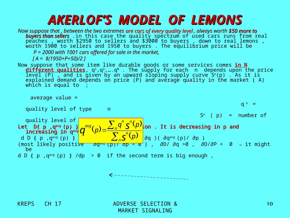
AKERLOF’S MODEL OF LEMONSAKERLOF’S MODEL OF LEMONSNow suppose that , between the two extremes Now suppose that , between the two extremes are cars of every quality levelare cars of every quality level , always worth , always worth

$50 more to buyers than sellers$50 more to buyers than sellers .in this case the quality spectrum of used cars runs from real peaches , worth $2950 to sellers and $3000 to buyers , down to real lemons , worth 1900 to sellers and 1950 to buyers . The equilibrium price will be

P = 2000 with 1001 cars offered for sale in the market, P = 2000 with 1001 cars offered for sale in the market, [ A = $(1950+P+50)/2 ] [ A = $(1950+P+50)/2 ] Now suppose that some item like durable goods or some services comes in N different

qualities, q1,q2,….qN . The supply for each n depends upon the price level (P) , and is given by an upward sloping supply curve Sn(p) . As it is explained demand depends on price (P) and average quality in the market ( A) which is equal to ;

average value = q n = quality level of type n Sn ( p) = number of quality level of type n Let DLet D(( p ,q p ,qavg avg (p) (p) )) be the demand function . It is decreasing in p and increasing in q be the demand function . It is decreasing in p and increasing in qavgavg(p).(p). d D ( p ,qavg (p) ) /dp = ∂D/∂P + ( ∂D/ ∂q )( ∂qavg (p)/ ∂p ) (most likely positive ∂qavg (p)/ ∂p > 0 ) , ∂D/ ∂q >0 , ∂D/∂P < 0 → it might be d D ( p ,qavg (p) ) /dp > 0 if the second term is big enough ,

n

n

nn

navg

p

pqp

ssq


11


It is possible that for some price levels lower than p* the slope of demand curve becomes positive [ d D( p ,qavg (p)/dp > 0 ] and does not intersect the supply curve as it is shown in the following figure . in these cases there will not be an equilibrium price and market breaks down as it is in some health insurance market .

quantity

pricedemand

supply

P*


12

SIGNALING QUALITY SIGNALING QUALITY In reality all manners of markets subject to adverse selection do function.

Why ? Often because the side to the transaction that has the superior side to the transaction that has the superior information will do something that indicates the quality of the good being information will do something that indicates the quality of the good being sold sold

1-1- in life insurance the high quality buyer distinguish himself from the low quality buyer and take actions that is not worthwhile for low quality buyer .

2-2- in used car market The high quality seller may take actions which distinguish him from the low quality seller and is not worthy for them .

with used carswith used cars ; aa- seller may offer partial warrantypartial warranty or b- b- may get the carcheckedchecked by an independent party . In life insuranceIn life insurance ; a-a- medical checkupsmedical checkups are sometimes required . Or ;b-b- golden age policygolden age policy may be used . No one will be turn down but only the benefits will greatly reduced for the beginning years of the benefits will greatly reduced for the beginning years of the insurance planinsurance plan . If the buyer of the insurance knows that he is dying soon , or if he wants to use the benefits very soon , he will not gain the whole benefit .


13

SIGNALING QUALITYSIGNALING QUALITYQuality seller and his actions are not worthwhile for low quality workers. One can think of adverse selection as an special case of moral hazard and

market signals as a special case of incentive schemes. The incentives could incentives could be direct or indirect ;be direct or indirect ;

1- direct incentives1- direct incentives ; the seller of the low quality car may be tossed into jail if he misrepresent the quality of car sold.

2- indirect incentives2- indirect incentives ; the seller of the used cars could be asked to give a six month warranty if he says that the car is peach. Or the buyer may offer $X if the seller offers him a warranty and $Y ( X>Y) , if he does not offer him a warranty .

The two classic model of adverse selection in the literature areThe two classic model of adverse selection in the literature are 1- SPENCE’S model of job market signaling and 1- SPENCE’S model of job market signaling and 2- ROTCHILD & STIGLITIZ model of insurance market2- ROTCHILD & STIGLITIZ model of insurance market . In the present analysis the job market model (Spence’s setting )will be used to

illustrate both cases.Imagine a population of workers with two qualitiespopulation of workers with two qualities with equal numbers ;with equal numbers ;First – high qualityFirst – high quality with high innate ability , denoting t=2t=2Second – low qualitySecond – low quality with low innate ability , denoting with t=1 t=1


14

SIGNALING QUALITYSIGNALING QUALITY There are firms that will hire the workers and operates in competitive

market and making zero pure profit.

Before going to Before going to workwork workers seek education that enhances their workers seek education that enhances their productivity. But education can not move workers from low to productivity. But education can not move workers from low to high quality level ,because it is intrinsichigh quality level ,because it is intrinsic.. Each worker chooses a Each worker chooses a level of education from a set say from level of education from a set say from e=0 to e=16e=0 to e=16 (the numbers of schooling).

A worker of type A worker of type t ( t=1 , 2)t ( t=1 , 2) and with education level of and with education level of e ( e=1 , … 16 )e ( e=1 , … 16 ) worth teworth te to a firm .note that for every level of education higher to a firm .note that for every level of education higher quality worker worth twice as much as lower quality onesquality worker worth twice as much as lower quality ones . FirmsFirms when they hire a worker are unable to tell whether the worker is able when they hire a worker are unable to tell whether the worker is able or notor not . . But they do get to see the worker’s CV and learn how many years they have gone to school and make wages contingent on the number of years they have spent in school .

Workers dislike educationWorkers dislike education , and less able dislike education more . Workers also want higher wages to be sure . Workers want to Workers want to maximize the following utility . maximize the following utility .


15

SIGNALING QUALITYSIGNALING QUALITYMax U=Ut ( w , e ) ; where “w” is wage rate ,“e” is the education level

and “t” is the type of the worker.

Utility is strictly increasing in “w” ,increasing in “w” ,

and strictly decreasing in “e”decreasing in “e” .

Shape of the worker’s indifference curve ;Shape of the worker’s indifference curve ;

w

Education level

Wag

e pa

id

Indifference curve of low ability workers

Indifference curve of high ability workers

Direction of Direction of increasing increasing preferencepreference

e

Worker’s indifference curve is the locus of the combination of wage and education level which brings a constant utility level . It is upward sloping and strictly convex. Take any point like P (or any other point). Notice that at least one indifference curve for low ability worker and one indifference curve for high ability worker would pass from this point The indifference The indifference curve of high ability worker shows a curve of high ability worker shows a higher level of utility than low ability higher level of utility than low ability one at any point like P one at any point like P .To compensate a worker for a given increase in education requires a greater increase in wages for a low ability worker than for a high ability worker. So , the indifference curve of the low ability worker is always more steeply sloped than high ability.

P


16

SIGNALING QUALITYSIGNALING QUALITYThis assumptionassumption known as a single-crossingsingle-crossing propertyproperty. For example ;

UUtt ( w , e ) = f(w) – K ( w , e ) = f(w) – Ktt g(e) g(e) , where ; f(w)f(w) is increasing and concave function , g(e)g(e) is increasing and strictly convex function , KKtt is positivepositive constant with KK22 >K >K11 . .

What would happen if the ability of workers were observable ability of workers were observable (full full information modelinformation model ) ). The high ability workershigh ability workers with education level ee would be paid paid 2e2e , while the low ability workerlow ability worker with the same education level would be paid ee . As showed in the figure in page 17 the high and low ability workers will pick different education pick different education levels which maximizes their utility levels given these wages .levels which maximizes their utility levels given these wages .

In the equilibrium education level of high ability workers (eIn the equilibrium education level of high ability workers (e22 ) )

is greater than low ability workers (e is greater than low ability workers (e11). So the firm could ). So the firm could realize the type of the workers from their education levelrealize the type of the workers from their education level

But we have to deal with situations in whichwhich ability level is not ability level is not directly observabledirectly observable . We will consider two casesWe will consider two cases ;

1-1- First ; job market signaling (Spence model )First ; job market signaling (Spence model ) 2-2- Second ; worker self selection from a list of menu ( Rotchild Second ; worker self selection from a list of menu ( Rotchild

and Stigltiz model). and Stigltiz model).


17

SIGNALING QUALITY,SIGNALING QUALITY, ability of workers are observableability of workers are observable

Education level

Wag

e pa

id


Indifference curve of high ability workers

Direction of increasing preference

e

W=eW=e

W=2eW=2e

ee11 ee22

The low ability worker knows that he should move on the W=e line and the high ability worker knows that he should move on the W=2e line, because the ability is observable by the firm . In other words each worker knows that his ablity is observable and he can not hide it . So , what he does is just a utility maximization concerning his constraint ( w=e or w=2e ).


18

SPENCE’S MODEL ; JOB MARKET SIGNALINGSPENCE’S MODEL ; JOB MARKET SIGNALING How many years Workers choose to go to school ?.They do so anticipatinganticipating some

wage function w(e)w(e) that gives wages for every level of education .Formally an equilibrium in the sense of Spence consist of ;an equilibrium in the sense of Spence consist of ; aa – an anticipated wage functionan anticipated wage function w(e)w(e) that workers anticipate will be paid to any

one obtaining this education level e e and , bb- probability distributionprobability distribution ππtt(e)(e) on the set of education levels for each type of

worker , t= 1 , 2 , such that the following two conditions are met ; bb11 - For each type t worker and education level e → e → ππtt(e)> (e)> 0 only if uut t [w(e) , e][w(e) , e] achieves the maximum value of uut t [w(e) , e][w(e) , e] over all ee Condition b1 says that based upon their anticipation , the workers choose that wage the workers choose that wage

level which maximizes their utility levellevel which maximizes their utility level bb22 - for each education level e e such that; ππ11(e) + (e) + ππ22(e)(e) > 0 ; w(e) = w(e) = ee [0.5[0.5ππ11(e) ](e) ] / [0.5/ [0.5ππ11(e) + 0.5(e) + 0.5ππ22(e)](e)] + + 2e2e [0.5[0.5ππ2 2 (e) ](e) ] / [0.5/ [0.5ππ11(e) + 0.5(e) + 0.5ππ22(e)](e)] ππtt(e) gives the proportion of type t workers(e) gives the proportion of type t workers who select education level ee in

equilibrium . So ππtt(e) is the probability of type t worker with education level of (e) is the probability of type t worker with education level of e .e . 0.5 = probability of type t in the population 0.5 = probability of type t in the population ((opulation of workers with two opulation of workers with two qualitiesqualities are assumed to be the same)are assumed to be the same)

Condition b2 express that in the equilibriumequilibrium which is attained under perfectperfect competitioncompetition , the wage rate , w(e) is equal to the conditional expected value of a worker presenting education level e. Since ability of workers are not observable , the eqilibrium wage should be represented in terms of expected wage (both of expected wage (both from workers and employers point of view). from workers and employers point of view). For the simplicity we assume that all the workers of a given type choose the same level of education :all the workers of a given type choose the same level of education :


19

SIGNALING QUALITYSIGNALING QUALITYTwo types of equilibrium - non observable quality (ability) ; Two types of equilibrium - non observable quality (ability) ;

1-First type ; separating (screening ) equilibrium ;1-First type ; separating (screening ) equilibrium ; All workers of type t=1 t=1 choose an education level ee1 1 .

All workers of type t=2t=2 choose an education level ee2 2 .Firms seeing the education level e1 , knowing the worker is of type 1 , pay a wage equal to e1 . And if they see the education level e2 , knowing the worker is of type 2 , pay a wage equal to 2e2 .

2-Second type ; pooling equilibrium2-Second type ; pooling equilibrium ; workers all pool at a single education level , e* , and the equilibrium wage will

be equal to ; firms by seeing educational level e* thinks that the probability of worker from type 1 or 2 is 1/2 .

w(e) = ( ew(e) = ( e** ) ( 1/2) + 2( e ) ( 1/2) + 2( e** ) ( 1/2) = 1.5 e ) ( 1/2) = 1.5 e* * { {ππ11(e) = (e) = ππ22(e) }(e) }

1-First type - Separating equilibrium (non observable 1-First type - Separating equilibrium (non observable quality);quality);

In order to have an separating equilibrium each type of workers will choose different level of education ; workers of workers of type 1type 1 would would rather rather choosechoose the wage education pair ( w=e the wage education pair ( w=e11 , e = e , e = e11 ) than ) than ( w = 2e( w = 2e2 2 ,e = e,e = e22 ) and vice versa ) and vice versa . Such an equilibrium could be seen in the following figure .


20

SIGNALING QUALITYSIGNALING QUALITY

Education level

Wag

e le

vel

W=2e

W=2e

W = eW = e

W(e) curve must lie W(e) curve must lie every where at or below every where at or below the indifference curves the indifference curves of the workers at the of the workers at the points that the workers points that the workers select because E and F select because E and F are the maximization are the maximization points; points; this is the self this is the self selection conditionselection condition . .

ee1 1 and e and e2 2 are are

education level which education level which are selected by low and are selected by low and high ability worker in the high ability worker in the equilibrium and equilibrium and observed by the firm as observed by the firm as a signala signal

Indifference curve of

high ability workers


e1 e2

point E on w(e) is selected by low ability worker , so indifference curve point E on w(e) is selected by low ability worker , so indifference curve of low ability worker and W=e line should pass through point E and of low ability worker and W=e line should pass through point E and point point F on w(e) is selected by high ability worker so indifference curve of high F on w(e) is selected by high ability worker so indifference curve of high ability worker and W=2e line should pass through point F ability worker and W=2e line should pass through point F

E

F

both kinds of labors will maximize their utility levels with respect to the expected wage constraint w(e) and solutions are E and F.


21

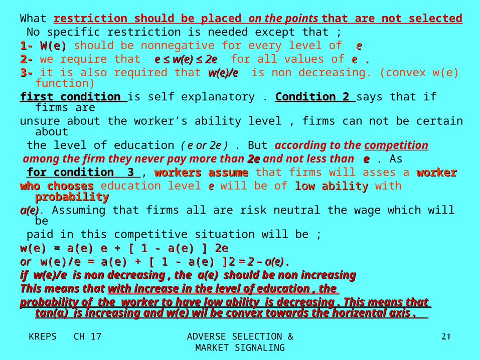
What restriction should be placed on the points that are not selected No specific restriction is needed except that ; 1-1- W(e)W(e) should be nonnegative for every level of ee2-2- we require that e ≤ w(e) ≤ 2ee ≤ w(e) ≤ 2e for all values of ee . .3-3- it is also required that w(e)/ew(e)/e is non decreasing. (convex w(e) function)first condition first condition is self explanatory . Condition 2 Condition 2 says that if firms are unsure about the worker’s ability level , firms can not be certain about the level of education ( e or 2ee or 2e ) . But according to the competition among the firm they never pay more than 2e2e and not less than e e . . As for condition 3 for condition 3 , workers assumeworkers assume that firms will asses a worker worker whowho chooses chooses education level ee will be of low abilitylow ability with probabilityprobabilitya(e)a(e). Assuming that firms all are risk neutral the wage which will be paid in this competitive situation will be ; w(e) = a(e) e + [ 1 - a(e) ] 2ew(e) = a(e) e + [ 1 - a(e) ] 2eor or w(e)/e = a(e) + [ 1 - a(e) ]2 w(e)/e = a(e) + [ 1 - a(e) ]2 = 2 – a(e) . = 2 – a(e) . if w(e)/e is non decreasing , the a(e) should be non increasing if w(e)/e is non decreasing , the a(e) should be non increasing This means that This means that with increase in the level of education , the with increase in the level of education , the probability of the worker to have low ability is decreasing . This probability of the worker to have low ability is decreasing . This

means that tan(means that tan(αα) is increasing and w(e) wil be convex towards ) is increasing and w(e) wil be convex towards the horizental axis . the horizental axis .


22


We could rephrase the condition 2 in the following manner ; a(e) is the probability of low ability worker choosing education level e . So firms firms

assessments given by a(e) are confirmed at education levels that assessments given by a(e) are confirmed at education levels that workers do select in the equilibrium ;workers do select in the equilibrium ; a(e) = [ 0.5 a(e) = [ 0.5 ππ11(e) ] / [ 0.5 (e) ] / [ 0.5 ππ11(e) + 0.5 (e) + 0.5 ππ2 2 (e) ] (e) ] ππtt(e) gives the proportion of type t workers(e) gives the proportion of type t workers who select education level ee in

equilibrium. population of workers with two qualities are in equal numbers ;

.Note that in the figure in slide no 20 the w(e) function does not liein slide no 20 the w(e) function does not lie between e and 2e .between e and 2e . So it does not satisfy condition (b) . In the following figure we introduce an equilibrium which satisfies introduce an equilibrium which satisfies

condition bcondition b..In this equilibrium the education level which is chosen by the worker is e^

1 . That is when w=e , the education level is equal to e^

1 . In other words the indifference curve of low ability worker is tangent to line w=e when e= e^

1 .In contrast to figure in slide no. 20 the low ability worker get higher utility in the equilibrium . low ability worker get higher utility in the equilibrium .


23


Education level

Wag

e le

vel

W=2e

W=2e

W=eW=e

W(e) curveW(e) curve

Indifference curve of Indifference curve of

high ability workershigh ability workers

Indifference curve of low Indifference curve of low ability workers which is ability workers which is higher than before . higher than before .

ee22ee^̂11 e1

24

Preposition 1 ; in any separating equilibrium for which the function w(e) satisfies condition Preposition 1 ; in any separating equilibrium for which the function w(e) satisfies condition (b) , low ability workers choose precisely e^(b) , low ability workers choose precisely e^1 1 and get the corresponding wages . In any and get the corresponding wages . In any equilibrium (separating or not) for which the function w(e) satisfies (b) , low ability workers equilibrium (separating or not) for which the function w(e) satisfies (b) , low ability workers get at least the utility that they get from get at least the utility that they get from ( w=e^( w=e^11 , e=e , e=e11 ) . (this is the utility level when ) . (this is the utility level when he introduce himself as low quality so in pooling equilibrium the utility level should he introduce himself as low quality so in pooling equilibrium the utility level should not be lower than this)not be lower than this)Pooling equilibriumPooling equilibrium ; ; in the pooling equilibrium we assume that all the workers choose a all the workers choose a single level of education say esingle level of education say e** . Numbers of high and low ability workers are the same and each have education e* .then a(e*) = 0.5 since ;a(e) = [ 0.5 a(e) = [ 0.5 ππ11(e) ] / [ 0.5 (e) ] / [ 0.5 ππ11(e)+0.5 (e)+0.5 ππ2 2 (e) ] , if (e) ] , if ππ11(e)= (e)= ππ2 2 (e) {pooling eqilibrium condition}, (e) {pooling eqilibrium condition}, then a(e) =1/2 then a(e) =1/2 w(e) = a(e) e + [ 1 - a(e) ] 2e → w(e*) = 1.5 e* w(e) = a(e) e + [ 1 - a(e) ] 2e → w(e*) = 1.5 e* workers assumeworkers assume that firms will asses a worker whoworker who chooses chooses education level ee will be of low low abilityability with probability probability a(e)a(e)

ππtt(e) gives the proportion of type t workers(e) gives the proportion of type t workers who select education level ee in equilibriumAn equilibrium of this sort is given by the following figure in slide no. 25slide no. 25 .note that the .note that the function w(e) has a kink at the pooling point function w(e) has a kink at the pooling point . This is necessary . Without the kink , we could not have w(e) underneath both types of indifference curves and touching those curves at pooling point . As we can see point E could be anywhere on the w=1.5e* As we can see point E could be anywhere on the w=1.5e* line and line and there could be many equilibrium there could be many equilibrium . .


25



Education level

Wag

e le

vel

W=2e

W=2e

W=eW=e

W(e) curveW(e) curve



Indifference curve of low Indifference curve of low ability workers which is ability workers which is higher than before . higher than before .

W=1.5eW=1.5e

ee**

EE


26

Rothschild and Stiglitz model ;Rothschild and Stiglitz model ;Workers self selection from a model ;Workers self selection from a model ;

The previous assumptions are holding ; that is ;

1- two types of workers ( low and high ability ) in equal numbers .

2- πi(e) = probability of choosing education level e by worker of type i . Proportion of i workers who choose education level e .

In the Spence model workers choose education levels in anticipation of offers from the firm , w(e) , and we assume that those anticipation are correct , at least for the education levels actually selected. Let’s turned this around and suppose that the firms moves first.

Suppose that the firms offer to workers a number of contracts of theSuppose that the firms offer to workers a number of contracts of the

form ( w, e ) before the workers go off to schoolform ( w, e ) before the workers go off to school , content in the

knowledge of what wage they will get once the school is done

( assuming they complete the number of years for which they have

contracted) . (We could also think of insurance market insteadWe could also think of insurance market instead with

insurance contracts being offered to people before hand). The

context with which the model is dealing . Now consider an equilibrium

in This context . An equilibrium in the context of Rothchild and Stiglitz An equilibrium in the context of Rothchild and Stiglitz

consist of ;consist of ;


27

SIGNALING QUALITYSIGNALING QUALITY a- a menu of contractsa- a menu of contracts , a set of pairs [ ( w( w11, e, e11) , ( w) , ( w22 , e , e22), … , (w), … , (wkk,e,ekk)) ]For some finite integer . And b- b- a selection rulea selection rule by which workers are assigned to contracts or , for each type of workers ( t ) a probability distribution type of workers ( t ) a probability distribution ππtt over [1,2,3,…k], over [1,2,3,…k], that satisfy three conditions as follows ; that satisfy three conditions as follows ; (1)(1) – – Each type of worker are assigned to the contract that is best for Each type of worker are assigned to the contract that is best for That worker in the menuThat worker in the menu . In symbols , πt(j) > 0 only if ut(wj , ej ) achieves the maximum of ut (wj’ , ej’ ) for j’ = 1,2,….k and t = 1,2 . ((2)2) – Each contract in the menu to which workers are assigned at least breaks Each contract in the menu to which workers are assigned at least breaks

even on averageeven on average. Otherwise , firms offering that contract would withdraw from the contract . In other words wage offered by firm is not greater than

the average anticipated wage level . In symbols for each j = 1,2,3,…k if π 1(j) + π2(j) > 0 , then ;WWjj

≤ [ 0.5 ≤ [ 0.5 ππ11(j) ]/[0.5 (j) ]/[0.5 ππ11(j) + 0.5 (j) + 0.5 ππ22(j) ] e(j) ] ejj + [ 0.5 + [ 0.5 ππ22(j) ]/[0.5 (j) ]/[0.5 ππ11(j) + 0.5 (j) + 0.5 ππ22(j) ] 2 e(j) ] 2 ejj (3)(3) – – No contract can be created that if offered in addition to those in No contract can be created that if offered in addition to those in the menu would make strictly positive profits for the firm offering it , the menu would make strictly positive profits for the firm offering it , assuming that workers choose among contracts in a manner consistent with rule (1) .


28

SIGNALING QUALITYSIGNALING QUALITYPreposition 2 – In an equilibrium , any contract that is taken up by Preposition 2 – In an equilibrium , any contract that is taken up by workers must earn precisely zero expected profit per worker workers must earn precisely zero expected profit per worker (competition leads the profit towards zero). (competition leads the profit towards zero).

Suppose that (w’ , e’ ) is offered and it is taken by some workers , and earns an expected profit of ε for the firm per worker who take it . Thenbecause of competition among the firms there could be some firms Which offers an amount equal to ( w’ + ε/2 ,e’). This new contract willattract the workers who previously were attracted by (w’ , e’ ) and will still return a profit of ε/2 , which is contradicting the condition 3 . Now assume that the new contract may attract others besides thoseNow assume that the new contract may attract others besides thosewho previously took (w’ , e’ )who previously took (w’ , e’ ) and those others may render theprofitability of this contract. If the new workers are low ability workersthese low ability workers may be able to render the profitability of new contract and the contradiction with condition 3 could be wipe out . But if But if the new workers are high-ability workersthe new workers are high-ability workers , then it could be shown that ; then it could be shown that ;

Proposition 3 ; there could not exist a pooling equilibrium ; Proposition 3 ; there could not exist a pooling equilibrium ;


29


Education level

Wag

e le

vel

W=2e

W=2e

W=eW=e



Indifference curve of low Indifference curve of low ability workers . ability workers .

W=1.5eW=1.5e

ee**

EE1.5 1.5 ee**

e’e’

W’W’

equilibrium point E (contract E) is chosen among different points (different contracts ) because it has the highest utililty among four different dotted points


30

SIGNALING QUALITYSIGNALING QUALITYSuppose that the firm are offering a menufirm are offering a menu of contracts that causes all

the workers to choose (1.5 e(1.5 e* * ,, ee** ) ) as shown in the figure . In the figure in page 29 the filled-in dots29 the filled-in dots are the menu of contracts that we suppose

Are offered . As it is seen the (1.5 e* , e* ) contract is the best , because theutility levels are higher .

From this position , any one of the firms can offer the contract (w’ , e’ ) one of the firms can offer the contract (w’ , e’ ) that is shown as a filled triangle . This is a contract that has a slightly

higher wages and education levels than (1.5 e* , e* ) , where theincreased wages more than compensate a high-ability worker but don’tcompensate a low-ability worker relative to the pooling contract. It willIt will

only attract the high ability workers . All the low ability workers prefer theonly attract the high ability workers . All the low ability workers prefer the(1.5 e(1.5 e* * ,, ee** ) contract . ) contract .

But if all high ability workers flock to ( w’ , e’ ) contract and non of low ability workers do so , then each worker who chooses ( w’ , e’ ) worth

2e’ to the firm that makes this offer . The firm makes a profit and The firm makes a profit and according to proposition 2 we can not have a pooling equilibrium.according to proposition 2 we can not have a pooling equilibrium. From this

point we can reach to the following proposition ;Proposition 4 . It is impossible , in eqilibrium , that any contract (w , e) Proposition 4 . It is impossible , in eqilibrium , that any contract (w , e)

is taken by positive fractions of high- and low ability workers both. So , is taken by positive fractions of high- and low ability workers both. So , only possible equilibrium is separating equilibriumonly possible equilibrium is separating equilibrium . .


31

SIGNALING QUALITYSIGNALING QUALITYProposition 5 ; There is only a single candidate for a separatingProposition 5 ; There is only a single candidate for a separating

equilibrium . In this candidate equilibrium . Low-ability workers choose equilibrium . In this candidate equilibrium . Low-ability workers choose the contract ( w=ethe contract ( w=e ^̂

11 , e=e , e=e^̂11 ) , where e ) , where e^̂

11 is defined as before ( page 23) and is defined as before ( page 23) andHigh-ability worker get w=2f High-ability worker get w=2f ^̂

22 , e= f , e= f ^̂2 2 , (page 33) , (page 33)

First let us concentrate on page 33 and on the first part of the proposition . If low ability workers are separated and choosing any other contractIf low ability workers are separated and choosing any other contract other

than ( w=ethan ( w=e^̂11 , e=e , e=e^̂

11 ) ) , a firm could add to the menu of contracts a contractlike ( w=e^

1 – δ , e=e^1 ) for δ>0 small enough so that the low ability

workers prefers this to the contract they are choosing now (otherthan ( w=e^

1 , e=e^1 ) ) in the supposed equilibrium . But then for any value

of δ>0 , this contract must be profitable . For explaining the second part of the proposition we should consider the f ^

2

which solve the maximization of u2(2e , e ) subject to e≥ f ^1 . That is That is f f ^̂

2 2 is is the education level that high-ability workers would choose if they could the education level that high-ability workers would choose if they could

have any point along the ray w=2e for e ≥ f have any point along the ray w=2e for e ≥ f ^̂11 . We want education level to . We want education level to

be greater than low ability worker when w=2e, because we expect high be greater than low ability worker when w=2e, because we expect high ability workers get higher education than low ability workers and separate ability workers get higher education than low ability workers and separate

themselves from them. themselves from them.


32

SIGNALINAG QUALITYSIGNALINAG QUALITY

Let’s now concentrate on the high-ability workers and the high-ability workers and

show that high quality workers get (w=2 f show that high quality workers get (w=2 f ^̂22 , e= f , e= f ^̂

22 ). ).

Why ? Why ? If high quality workers are separated by any other contract

other than (w=2 f ^2 , e= f ^

2 ) , some firm could offer a

contract like (w=2 f ^2 - δ , e= f ^

2 ) that for sufficiently

small δ would be more attractive to high ability workers than the contract they are taking at the supposed equilibrium .

Since f Since f ^̂22 ≥ f ≥ f ^̂

11 , this contract is less appealing than the , this contract is less appealing than the contract ( w = econtract ( w = e^̂

11 , e = e , e = e^̂11 ) for low ability workers ) for low ability workers

(lower utility level for low ability workers ). Hence this (lower utility level for low ability workers ). Hence this contract will precisely attract the high ability workers contract will precisely attract the high ability workers and thus for any and thus for any δδ >0 , this contract is precisely >0 , this contract is precisely profitable . profitable .


33


Education level

Wag

e le

vel

W=2e

W=2e

W=eW=e


ee^̂11

EE

Indifference curve of high ability Indifference curve of high ability

workers .workers .

f f ^̂11 = f = f ^̂

22e’e’

w’w’

W = 1.5 eW = 1.5 e

Considering the figure in page 33 we have there depicted separating equilibrium in a case where f ^

2 = f ^1 . It could It could

be shown that no firm would try to break this equilibrium be shown that no firm would try to break this equilibrium point by offering a contract in a position such as (w’ , e’ ) point by offering a contract in a position such as (w’ , e’ ) that is shown with w’ a bit less than 2e’ and e’ a bit less that is shown with w’ a bit less than 2e’ and e’ a bit less than f than f ^̂

11 (point E lies above the w=1.5e line ). (point E lies above the w=1.5e line ). This contract when added to the menu would certainly attract the high attract the high ability workersability workers because it offers them a higher utilityhigher utility level than the one they are enjoying with ( w=2f ^

2 e= f ^2 )

contract . Every high ability worker would be profitable at Every high ability worker would be profitable at this contract because wage is less than 2e’ .this contract because wage is less than 2e’ . But this will But this will also attract the low ability workersalso attract the low ability workers because the utility level of low ability workers are also higher than the one which they are enjoying now . Now in this pooling equilibrium the firm should pay a wage less than 1.5e’ to earn a profit firm should pay a wage less than 1.5e’ to earn a profit which is not the case in the figure. which is not the case in the figure. Now consider the figure in page 35 in which point E located page 35 in which point E located below the w=1.5e line . below the w=1.5e line .


34



35


Education level

Wag

e le

vel

W=2e

W=2e

W=eW=e


ee^̂11

EE

Indifference curve of high ability Indifference curve of high ability

workers .workers .

f f ^̂11 = f = f ^̂

22e’e’

w’w’

W=1.5eW=1.5e


36

In page 35 the indifference curve of the high ability workers through the point ( w=2 f^

2 , e= f^2 ) dips below the line w= 1.5e. In this case a firm

could offer a contract such as (w’ , e’ )as shown below the line w=1.5e , but still above the high-ability worker’s indifference curve . This would break the equilibrium , because even though it attracts all the workers , high ability and low ability , it is still profitable .So there can not be an equilibrium at all . Any sort of pooling is inconsistent with the equilibrium , (as proved by proposition 3). And the only possible separating equilibrium can also be broken .. Proposition 6 ; Proposition 6 ; In the formation of Rothschild and Stiglitz , there is at most one In the formation of Rothschild and Stiglitz , there is at most one equilibrium. In the candidate equilibrium , low ability workers choose equilibrium. In the candidate equilibrium , low ability workers choose ( w=e ( w=e^̂

11 , e=e , e=e^̂11 ) and high ability worker choose the education level ) and high ability worker choose the education level

f f ^̂2 2 . Such that ( w=2f . Such that ( w=2f ^̂

22 e= f e= f ^̂2 2 ) is their most preferred point along the ) is their most preferred point along the

ray w=2e for e≥ f ray w=2e for e≥ f ^̂11 . If the indifference curve for high ability workers . If the indifference curve for high ability workers

through the point ( w=2f through the point ( w=2f ^̂22 e= f e= f ^̂

2 2 ) dips below the pooling line w=1.5e, ) dips below the pooling line w=1.5e, then there is no equilibrium at all .if this indifference curve stays then there is no equilibrium at all .if this indifference curve stays above ( or just touch) the pooling line , then this single candidate above ( or just touch) the pooling line , then this single candidate equilibrium is an only equilibrium equilibrium is an only equilibrium ..


SIGNALINAG QUALITYSIGNALINAG QUALITYThe stories of Riley and Wilson The stories of Riley and Wilson In many markets where signaling takes place , such as insurance , it seems natural to suppose that uninformed parties put a menu of offers on the table from which informed parties must choose. So conclusion of Rothchild and Stiglitz analysis , namely that there may be no equilibrium at all , is rather troublesome . A number of authors have suggested that the problem lies in the notion of equilibrium proposed by Rothchild and Stiglitz . Two of the writers are Riely and Wilson .

RileyRiley advocates the notion of reactive equilibrium reactive equilibrium , , in which to destroy a proposed equilibrium , it must be possible to add a contract to the menu that will be strictly profitable and that will not become strictly unprofitable if other firms allowed to add still more contracts to the menu . In this sort of scheme , our argument for why there are no pooling equilibrium stands up ; we broke a pooling equilibrium by adding a contract that attracted high-ability workers only . Given that the pooling contract remained to attract low-ability workers . There is no way to make this pool-breaking contract strictly unprofitable as long as the old pooling contract is remains , because as long

as the old KREPS CH 17 ADVERSE SELECTION & MARKET SIGNALING

37

SIGNALINAG QUALITYSIGNALINAG QUALITYPooling contract is present , only the high ability workers would ever consider taking the new contract . But you are at much more risk when adding a contract that attempts to break a separating equilibrium by pooling high and low ability workers . For in this case , still another contract can be added that siphons from your contract the high ability workers , leaving you with only low ability workers . Hence , Riley concludes that reactive equilibrium always exist , and they correspond to the single candidate separating equilibrium .

WilsonWilson , on the other hand , proposed a notion called anticipatory anticipatory equilibrium.equilibrium. In this case , to break a proposed equilibrium it must be possible to add a contract that is strictly profitable and that does not become strictly unprofitable when unprofitable contracts from the original menu are withdrawn . Now if you try to break a pooling equilibrium by skimming the high ability workers , you are at risk ; the pooling contract that you destroy becomes unprofitable because after your addition it attracts only low ability workers . But if it is withdrawn , all those low ability workers may flock to your contract . On the other hand if you break a separating equilibrium with a pooling contract , you are not at risk ; because you have created a contract that attracts all the workers , You do not care if other, now unused contracts are withdrawn

ADVERSE SELECTION & MARKET SIGNALING

38

SIGNALINAG QUALITYSIGNALINAG QUALITYSo, Wilson concludes , anticipatory equilibrium always exist ; So, Wilson concludes , anticipatory equilibrium always exist ; sometimes there is more than one ; and pooling is possible as an sometimes there is more than one ; and pooling is possible as an equilibrium outcome equilibrium outcome .

How do we sort between Rothschild and How do we sort between Rothschild and Stiglitz , Riley , and Wilson ? Stiglitz , Riley , and Wilson ?

Think in Terms of an insurance market that is regulated by some regulatory authorities . If you think that firms can not withdraw contracts can not withdraw contracts because the regulatory committee forbid this , then Riley’s equilibriuRiley’s equilibrium concept seems the more reasonable .

If you think that the regulatory authorities permit the firms to withdraw unprofitable contracts and are very tough on adding contracts that potentially affect the profitability of others , then Wilson’s notion seems more reasonable .

As for Rothcilds and Stiglitz , think of regulators who call for firms to register simultaneously and independently the contracts they wish to offer , with no room to add or subtract subsequently.


39

KREPS CH 17ADVERSE SELECTION & MARKET SIGNALING 1INTRODUCTIONINTRODUCTION Greshman’s Law...

Documents

Transcript of KREPS CH 17ADVERSE SELECTION & MARKET SIGNALING 1INTRODUCTIONINTRODUCTION Greshman’s Law...