Kreith F.; Berger, S.A.; et. al. Fluid Mechanics Mechanical … ENGINEERING... · Fluid Mechanics...
209
Kreith, F.; Berger, S.A.; et. al. “Fluid Mechanics” Mechanical Engineering Handbook Ed. Frank Kreith Boca Raton: CRC Press LLC, 1999 c 1999 by CRC Press LLC
Transcript of Kreith F.; Berger, S.A.; et. al. Fluid Mechanics Mechanical … ENGINEERING... · Fluid Mechanics...

Kreith, F.; Berger, S.A.; et. al. “Fluid Mechanics”Mechanical Engineering HandbookEd. Frank KreithBoca Raton: CRC Press LLC, 1999
c©1999 by CRC Press LLC
Fluid Mechanics*
3.1 Fluid Statics......................................................................3-2Equilibrium of a Fluid Element ¥ Hydrostatic Pressure ¥ Manometry ¥ Hydrostatic Forces on Submerged Objects ¥ Hydrostatic Forces in Layered Fluids ¥ Buoyancy ¥ Stability of Submerged and Floating Bodies ¥ Pressure Variation in Rigid-Body Motion of a Fluid
3.2 Equations of Motion and Potential Flow ......................3-11Integral Relations for a Control Volume ¥ Reynolds Transport Theorem ¥ Conservation of Mass ¥ Conservation of Momentum ¥ Conservation of Energy ¥ Differential Relations for Fluid Motion ¥ Mass ConservationÐContinuity Equation ¥ Momentum Conservation ¥ Analysis of Rate of Deformation ¥ Relationship between Forces and Rate of Deformation ¥ The NavierÐStokes Equations ¥ Energy Conservation Ñ The Mechanical and Thermal Energy Equations ¥ Boundary Conditions ¥ Vorticity in Incompressible Flow ¥ Stream Function ¥ Inviscid Irrotational Flow: Potential Flow
3.3 Similitude: Dimensional Analysis and Data Correlation.............................................................3-28Dimensional Analysis ¥ Correlation of Experimental Data and Theoretical Values
3.4 Hydraulics of Pipe Systems...........................................3-44Basic Computations ¥ Pipe Design ¥ Valve Selection ¥ Pump Selection ¥ Other Considerations
3.5 Open Channel Flow .......................................................3-61DeÞnition ¥ Uniform Flow ¥ Critical Flow ¥ Hydraulic Jump ¥ Weirs ¥ Gradually Varied Flow
3.6 External Incompressible Flows......................................3-70Introduction and Scope ¥ Boundary Layers ¥ Drag ¥ Lift ¥ Boundary Layer Control ¥ Computation vs. Experiment
3.7 Compressible Flow.........................................................3-81Introduction ¥ One-Dimensional Flow ¥ Normal Shock Wave ¥ One-Dimensional Flow with Heat Addition ¥ Quasi-One-Dimensional Flow ¥ Two-Dimensional Supersonic Flow
3.8 Multiphase Flow.............................................................3-98Introduction ¥ Fundamentals ¥ GasÐLiquid Two-Phase Flow ¥ GasÐSolid, LiquidÐSolid Two-Phase Flows
* Nomenclature for Section 3 appears at end of chapter.
Frank KreithUniversity of Colorado
Stanley A. BergerUniversity of California, Berkeley
Stuart W. ChurchillUniversity of Pennsylvania
J. Paul TullisUtah State University
Frank M. WhiteUniversity of Rhode Island
Alan T. McDonaldPurdue University
Ajay KumarNASA Langley Research Center
John C. ChenLehigh University
Thomas F. Irvine, Jr.State University of New York, Stony Brook
Massimo CapobianchiState University of New York, Stony Brook
Francis E. KennedyDartmouth College
E. Richard BooserConsultant, Scotia, NY
Donald F. WilcockTribolock, Inc.
Robert F. BoehmUniversity of Nevada-Las Vegas
Rolf D. ReitzUniversity of Wisconsin
Sherif A. SherifUniversity of Florida
Bharat BhushanThe Ohio State University
3-1© 1999 by CRC Press LLC
3
-2
Section 3
3.9 Non-Newtonian Flows .................................................3-114Introduction ¥ ClassiÞcation of Non-Newtonian Fluids ¥ Apparent Viscosity ¥ Constitutive Equations ¥ Rheological Property Measurements ¥ Fully Developed Laminar Pressure Drops for Time-Independent Non-Newtonian Fluids ¥ Fully Developed Turbulent Flow Pressure Drops ¥ Viscoelastic Fluids
3.10 Tribology, Lubrication, and Bearing Design...............3-128Introduction ¥ Sliding Friction and Its Consequences ¥ Lubricant Properties ¥ Fluid Film Bearings ¥ Dry and Semilubricated Bearings ¥ Rolling Element Bearings ¥ Lubricant Supply Methods
3.11 Pumps and Fans ...........................................................3-170Introduction ¥ Pumps ¥ Fans
3.12 Liquid Atomization and Spraying................................3-177Spray Characterization ¥ Atomizer Design Considerations ¥ Atomizer Types
3.13 Flow Measurement.......................................................3-186Direct Methods ¥ Restriction Flow Meters for Flow in Ducts ¥ Linear Flow Meters ¥ Traversing Methods ¥ Viscosity Measurements
3.14 Micro/Nanotribology....................................................3-197Introduction ¥ Experimental Techniques ¥ Surface Roughness, Adhesion, and Friction ¥ Scratching, Wear, and Indentation ¥ Boundary Lubrication
3.1 Fluid Statics
Stanley A. Berger
Equilibrium of a Fluid Element
If the sum of the external forces acting on a ßuid element is zero, the ßuid will be either at rest ormoving as a solid body Ñ in either case, we say the ßuid element is in equilibrium. In this section weconsider ßuids in such an equilibrium state. For ßuids in equilibrium the only internal stresses actingwill be normal forces, since the shear stresses depend on velocity gradients, and all such gradients, bythe deÞnition of equilibrium, are zero. If one then carries out a balance between the normal surfacestresses and the body forces, assumed proportional to volume or mass, such as gravity, acting on anelementary prismatic ßuid volume, the resulting equilibrium equations, after shrinking the volume tozero, show that the normal stresses at a point are the same in all directions, and since they are knownto be negative, this common value is denoted by Ðp, p being the pressure.
Hydrostatic Pressure
If we carry out an equilibrium of forces on an elementary volume element dxdydz, the forces beingpressures acting on the faces of the element and gravity acting in the Ðz direction, we obtain
(3.1.1)
The Þrst two of these imply that the pressure is the same in all directions at the same vertical height ina gravitational Þeld. The third, where g is the speciÞc weight, shows that the pressure increases withdepth in a gravitational Þeld, the variation depending on r(z). For homogeneous ßuids, for which r =constant, this last equation can be integrated immediately, yielding
¶¶
¶¶
¶¶
r gp
x
p
y
p
zg= = = - = -0, and
© 1999 by CRC Press LLC
Fluid Mechanics
3
-3
(3.1.2)
or
(3.1.3)
where h denotes the elevation. These are the equations for the hydrostatic pressure distribution.When applied to problems where a liquid, such as the ocean, lies below the atmosphere, with a
constant pressure patm, h is usually measured from the ocean/atmosphere interface and p at any distanceh below this interface differs from patm by an amount
(3.1.4)
Pressures may be given either as absolute pressure, pressure measured relative to absolute vacuum,or gauge pressure, pressure measured relative to atmospheric pressure.
Manometry
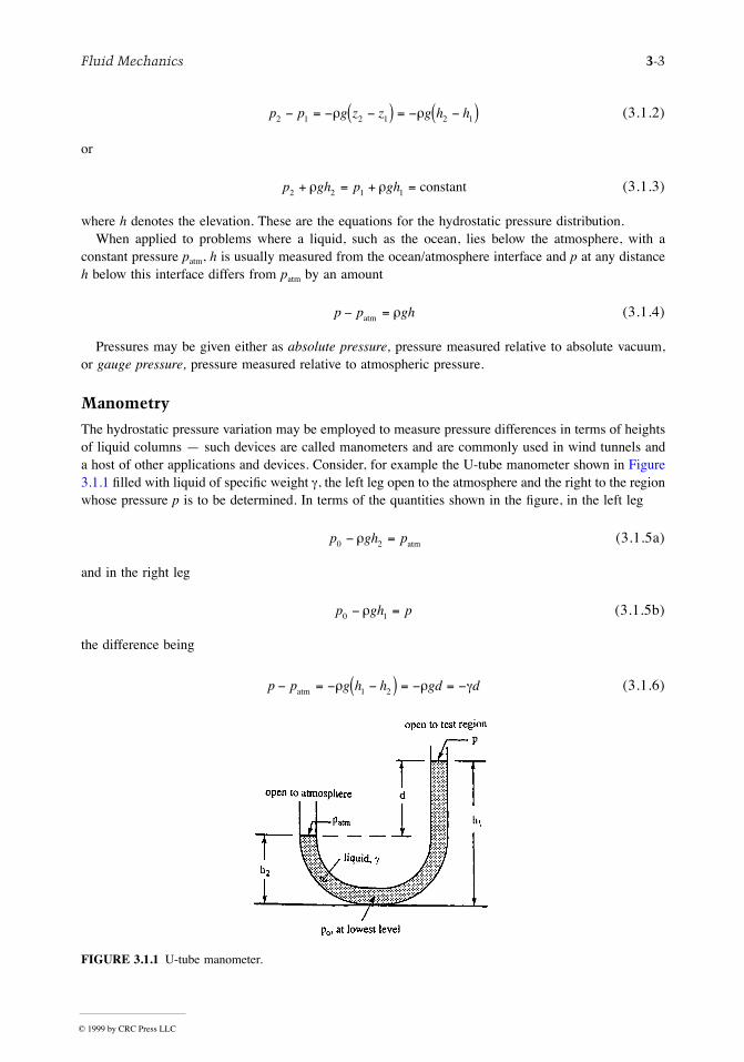
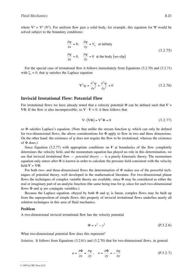
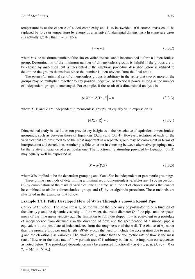
The hydrostatic pressure variation may be employed to measure pressure differences in terms of heightsof liquid columns Ñ such devices are called manometers and are commonly used in wind tunnels anda host of other applications and devices. Consider, for example the U-tube manometer shown in Figure3.1.1 Þlled with liquid of speciÞc weight g, the left leg open to the atmosphere and the right to the regionwhose pressure p is to be determined. In terms of the quantities shown in the Þgure, in the left leg
(3.1.5a)
and in the right leg
(3.1.5b)
the difference being
(3.1.6)
FIGURE 3.1.1 U-tube manometer.
p p g z z g h h2 1 2 1 2 1- = - -( ) = - -( )r r
p gh p gh2 2 1 1+ = + =r r constant
p p gh- =atm r
p gh p0 2- =r atm
p gh p0 1- =r
p p g h h gd d- = - -( ) = - = -atm r r g1 2
© 1999 by CRC Press LLC
3
-4
Section 3
and determining p in terms of the height difference d = h1 Ð h2 between the levels of the ßuid in thetwo legs of the manometer.
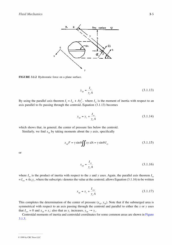
Hydrostatic Forces on Submerged Objects
We now consider the force acting on a submerged object due to the hydrostatic pressure. This is given by
(3.1.7)
where h is the variable vertical depth of the element dA and p0 is the pressure at the surface. In turn weconsider plane and nonplanar surfaces.
Forces on Plane Surfaces
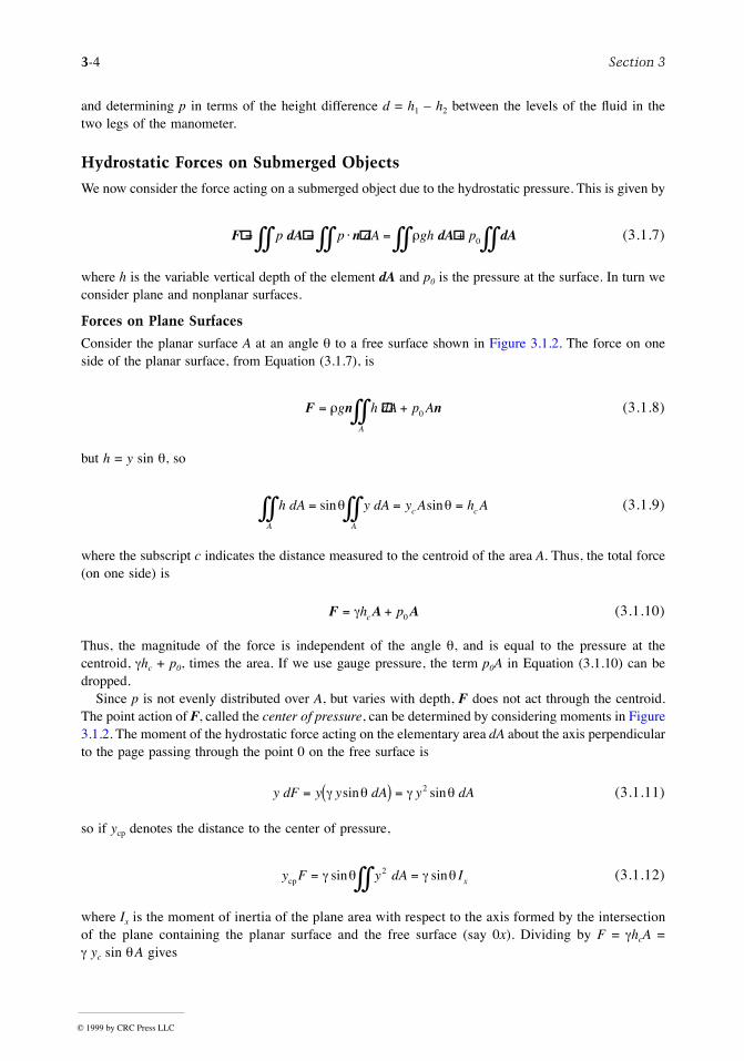
Consider the planar surface A at an angle q to a free surface shown in Figure 3.1.2. The force on oneside of the planar surface, from Equation (3.1.7), is
(3.1.8)
but h = y sin q, so
(3.1.9)
where the subscript c indicates the distance measured to the centroid of the area A. Thus, the total force(on one side) is
(3.1.10)
Thus, the magnitude of the force is independent of the angle q, and is equal to the pressure at thecentroid, ghc + p0, times the area. If we use gauge pressure, the term p0A in Equation (3.1.10) can bedropped.
Since p is not evenly distributed over A, but varies with depth, F does not act through the centroid.The point action of F, called the center of pressure, can be determined by considering moments in Figure3.1.2. The moment of the hydrostatic force acting on the elementary area dA about the axis perpendicularto the page passing through the point 0 on the free surface is
(3.1.11)
so if ycp denotes the distance to the center of pressure,
(3.1.12)
where Ix is the moment of inertia of the plane area with respect to the axis formed by the intersectionof the plane containing the planar surface and the free surface (say 0x). Dividing by F = ghcA =g yc sin qA gives
F dA n dA dA= = × = +òò òò òò òòp p dA gh pr 0
F n n= +òòrg h dA p A
A
0
h dA y dA y A h A
A A
c còò òò= = =sin sinq q
F A A= +gh pc 0
y dF y y dA y dA= ( ) =g q g qsin sin2
y F y dA Ixcp = =òòg q g qsin sin2
© 1999 by CRC Press LLC
Fluid Mechanics 3-5
(3.1.13)
By using the parallel axis theorem Ix = Ixc + where Ixc is the moment of inertia with respect to anaxis parallel to 0x passing through the centroid, Equation (3.1.13) becomes
(3.1.14)
which shows that, in general, the center of pressure lies below the centroid.Similarly, we Þnd xcp by taking moments about the y axis, speciÞcally
(3.1.15)
or
(3.1.16)
where Ixy is the product of inertia with respect to the x and y axes. Again, the parallel axis theorem Ixy
= Ixyc + Axcyc, where the subscript c denotes the value at the centroid, allows Equation (3.1.16) to be written
(3.1.17)
This completes the determination of the center of pressure (xcp, ycp). Note that if the submerged area issymmetrical with respect to an axis passing through the centroid and parallel to either the x or y axesthat Ixyc = 0 and xcp = xc; also that as yc increases, ycp ® yc.
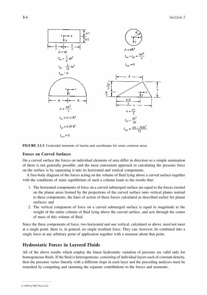
Centroidal moments of inertia and centroidal coordinates for some common areas are shown in Figure3.1.3.
FIGURE 3.1.2 Hydrostatic force on a plane surface.
yI
y Ax
ccp =
Ayc2 ,
y yI
y Acxc
ccp = +
x F xy dA Ixycp = =òòg q g qsin sin
xI
y Axy
ccp =
x xI
y Acxyc
ccp = +
© 1999 by CRC Press LLC
3-6 Section 3
Forces on Curved Surfaces
On a curved surface the forces on individual elements of area differ in direction so a simple summationof them is not generally possible, and the most convenient approach to calculating the pressure forceon the surface is by separating it into its horizontal and vertical components.
A free-body diagram of the forces acting on the volume of ßuid lying above a curved surface togetherwith the conditions of static equilibrium of such a column leads to the results that:
1. The horizontal components of force on a curved submerged surface are equal to the forces exertedon the planar areas formed by the projections of the curved surface onto vertical planes normalto these components, the lines of action of these forces calculated as described earlier for planarsurfaces; and
2. The vertical component of force on a curved submerged surface is equal in magnitude to theweight of the entire column of ßuid lying above the curved surface, and acts through the centerof mass of this volume of ßuid.
Since the three components of force, two horizontal and one vertical, calculated as above, need not meetat a single point, there is, in general, no single resultant force. They can, however, be combined into asingle force at any arbitrary point of application together with a moment about that point.
Hydrostatic Forces in Layered Fluids
All of the above results which employ the linear hydrostatic variation of pressure are valid only forhomogeneous ßuids. If the ßuid is heterogeneous, consisting of individual layers each of constant density,then the pressure varies linearly with a different slope in each layer and the preceding analyses must beremedied by computing and summing the separate contributions to the forces and moments.
FIGURE 3.1.3 Centroidal moments of inertia and coordinates for some common areas.
© 1999 by CRC Press LLC
Fluid Mechanics 3-7
Buoyancy
The same principles used above to compute hydrostatic forces can be used to calculate the net pressureforce acting on completely submerged or ßoating bodies. These laws of buoyancy, the principles ofArchimedes, are that:
1. A completely submerged body experiences a vertical upward force equal to the weight of thedisplaced ßuid; and
2. A ßoating or partially submerged body displaces its own weight in the ßuid in which it ßoats(i.e., the vertical upward force is equal to the body weight).
The line of action of the buoyancy force in both (1) and (2) passes through the centroid of the displacedvolume of ßuid; this point is called the center of buoyancy. (This point need not correspond to the centerof mass of the body, which could have nonuniform density. In the above it has been assumed that thedisplaced ßuid has a constant g. If this is not the case, such as in a layered ßuid, the magnitude of thebuoyant force is still equal to the weight of the displaced ßuid, but the line of action of this force passesthrough the center of gravity of the displaced volume, not the centroid.)
If a body has a weight exactly equal to that of the volume of ßuid it displaces, it is said to be neutrallybuoyant and will remain at rest at any point where it is immersed in a (homogeneous) ßuid.
Stability of Submerged and Floating Bodies
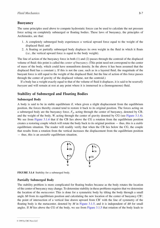
Submerged Body
A body is said to be in stable equilibrium if, when given a slight displacement from the equilibriumposition, the forces thereby created tend to restore it back to its original position. The forces acting ona submerged body are the buoyancy force, FB, acting through the center of buoyancy, denoted by CB,and the weight of the body, W, acting through the center of gravity denoted by CG (see Figure 3.1.4).We see from Figure 3.1.4 that if the CB lies above the CG a rotation from the equilibrium positioncreates a restoring couple which will rotate the body back to its original position Ñ thus, this is a stableequilibrium situation. The reader will readily verify that when the CB lies below the CG, the couplethat results from a rotation from the vertical increases the displacement from the equilibrium positionÑ thus, this is an unstable equilibrium situation.
Partially Submerged Body
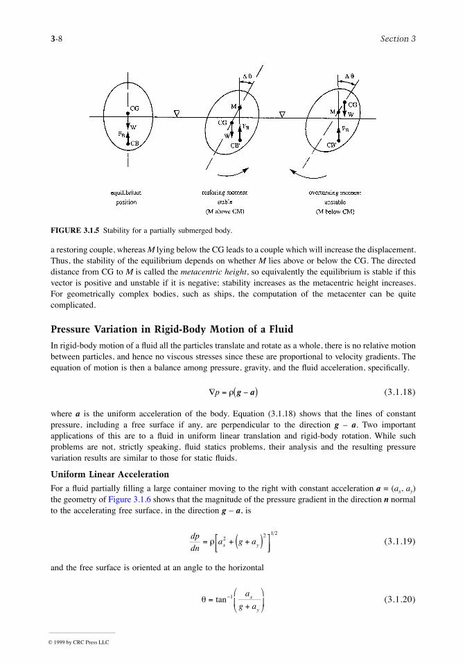
The stability problem is more complicated for ßoating bodies because as the body rotates the locationof the center of buoyancy may change. To determine stability in these problems requires that we determinethe location of the metacenter. This is done for a symmetric body by tilting the body through a smallangle Dq from its equilibrium position and calculating the new location of the center of buoyancy CB¢;the point of intersection of a vertical line drawn upward from CB¢ with the line of symmetry of theßoating body is the metacenter, denoted by M in Figure 3.1.5, and it is independent of Dq for smallangles. If M lies above the CG of the body, we see from Figure 3.1.5 that rotation of the body leads to
FIGURE 3.1.4 Stability for a submerged body.
© 1999 by CRC Press LLC
3-8 Section 3
a restoring couple, whereas M lying below the CG leads to a couple which will increase the displacement.Thus, the stability of the equilibrium depends on whether M lies above or below the CG. The directeddistance from CG to M is called the metacentric height, so equivalently the equilibrium is stable if thisvector is positive and unstable if it is negative; stability increases as the metacentric height increases.For geometrically complex bodies, such as ships, the computation of the metacenter can be quitecomplicated.
Pressure Variation in Rigid-Body Motion of a Fluid
In rigid-body motion of a ßuid all the particles translate and rotate as a whole, there is no relative motionbetween particles, and hence no viscous stresses since these are proportional to velocity gradients. Theequation of motion is then a balance among pressure, gravity, and the ßuid acceleration, speciÞcally.
(3.1.18)
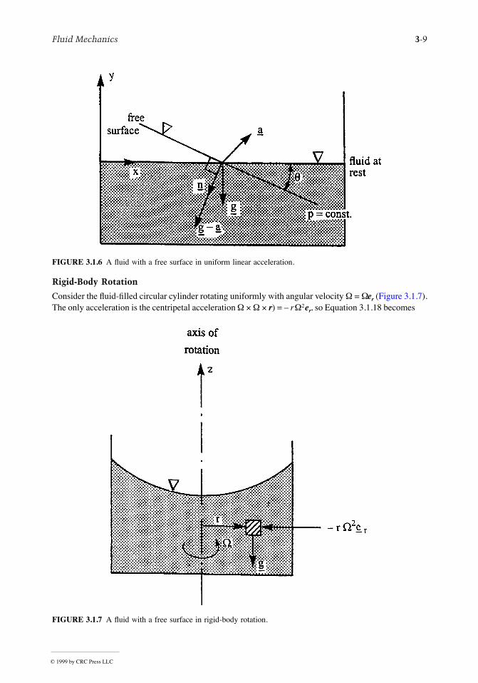
where a is the uniform acceleration of the body. Equation (3.1.18) shows that the lines of constantpressure, including a free surface if any, are perpendicular to the direction g Ð a. Two importantapplications of this are to a ßuid in uniform linear translation and rigid-body rotation. While suchproblems are not, strictly speaking, ßuid statics problems, their analysis and the resulting pressurevariation results are similar to those for static ßuids.
Uniform Linear Acceleration
For a ßuid partially Þlling a large container moving to the right with constant acceleration a = (ax, ay)the geometry of Figure 3.1.6 shows that the magnitude of the pressure gradient in the direction n normalto the accelerating free surface, in the direction g Ð a, is
(3.1.19)
and the free surface is oriented at an angle to the horizontal
(3.1.20)
FIGURE 3.1.5 Stability for a partially submerged body.
Ñ = -( )p r g a
dp
dna g ax y= + +( )é
ëêùûú
r 22 1 2
q =+
æ
èç
ö
ø÷
-tan 1 a
g ax
y
© 1999 by CRC Press LLC
Fluid Mechanics 3-9
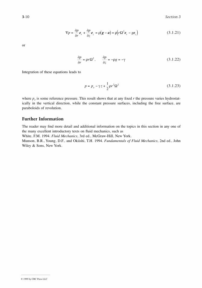
Rigid-Body Rotation
Consider the ßuid-Þlled circular cylinder rotating uniformly with angular velocity W = Wer (Figure 3.1.7).The only acceleration is the centripetal acceleration W ´ W ´ r) = Ð rW2er, so Equation 3.1.18 becomes
FIGURE 3.1.6 A ßuid with a free surface in uniform linear acceleration.
FIGURE 3.1.7 A ßuid with a free surface in rigid-body rotation.
© 1999 by CRC Press LLC
3-10 Section 3
(3.1.21)
or
(3.1.22)
Integration of these equations leads to
(3.1.23)
where po is some reference pressure. This result shows that at any Þxed r the pressure varies hydrostat-ically in the vertical direction, while the constant pressure surfaces, including the free surface, areparaboloids of revolution.
Further Information
The reader may Þnd more detail and additional information on the topics in this section in any one ofthe many excellent introductory texts on ßuid mechanics, such asWhite, F.M. 1994. Fluid Mechanics, 3rd ed., McGraw-Hill, New York.Munson, B.R., Young, D.F., and Okiishi, T.H. 1994. Fundamentals of Fluid Mechanics, 2nd ed., JohnWiley & Sons, New York.
Ñ = + = -( ) = -( )pp
r
p
zr gr z r z
¶¶
¶¶
r re e g a e eW2
¶¶
r¶¶
r gp
rr
p
zg= = - = -W2 ,
p p z ro= - +g r12
2 2W
© 1999 by CRC Press LLC
Fluid Mechanics 3-11
3.2 Equations of Motion and Potential Flow
Stanley A. Berger
Integral Relations for a Control Volume
Like most physical conservation laws those governing motion of a ßuid apply to material particles orsystems of such particles. This so-called Lagrangian viewpoint is generally not as useful in practicalßuid ßows as an analysis through Þxed (or deformable) control volumes Ñ the Eulerian viewpoint. Therelationship between these two viewpoints can be deduced from the Reynolds transport theorem, fromwhich we also most readily derive the governing integral and differential equations of motion.
Reynolds Transport Theorem
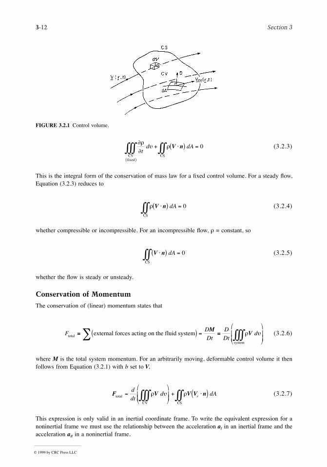
The extensive quantity B, a scalar, vector, or tensor, is deÞned as any property of the ßuid (e.g.,momentum, energy) and b as the corresponding value per unit mass (the intensive value). The Reynoldstransport theorem for a moving and arbitrarily deforming control volume CV, with boundary CS (seeFigure 3.2.1), states that
(3.2.1)
where Bsystem is the total quantity of B in the system (any mass of Þxed identity), n is the outward normalto the CS, Vr = V(r, t) Ð VCS(r, t), the velocity of the ßuid particle, V(r, t), relative to that of the CS,VCS(r, t), and d/dt on the left-hand side is the derivative following the ßuid particles, i.e., the ßuid masscomprising the system. The theorem states that the time rate of change of the total B in the system isequal to the rate of change within the CV plus the net ßux of B through the CS. To distinguish betweenthe d/dt which appears on the two sides of Equation (3.2.1) but which have different interpretations, thederivative on the left-hand side, following the system, is denoted by D/Dt and is called the materialderivative. This notation is used in what follows. For any function f(x, y, z, t),
For a CV Þxed with respect to the reference frame, Equation (3.2.1) reduces to
(3.2.2)
(The time derivative operator in the Þrst term on the right-hand side may be moved inside the integral,in which case it is then to be interpreted as the partial derivative ¶/¶t.)
Conservation of Mass
If we apply Equation (3.2.2) for a Þxed control volume, with Bsystem the total mass in the system, thensince conservation of mass requires that DBsystem/Dt = 0 there follows, since b = Bsystem/m = 1,
d
dtB
d
dtb d b dArsystem
CV CS
( ) =æ
èçç
ö
ø÷÷
+ ×( )òòò òòr u r V n
Df
Dt
f
tf= + × Ñ
¶¶
V
D
DtB
d
dtb d b dAsystem
CVfixed
CS
( ) = ( ) + ×( )
( )
òòò òòr u r V n
© 1999 by CRC Press LLC
3-12 Section 3
(3.2.3)
This is the integral form of the conservation of mass law for a Þxed control volume. For a steady ßow,Equation (3.2.3) reduces to
(3.2.4)
whether compressible or incompressible. For an incompressible ßow, r = constant, so
(3.2.5)
whether the ßow is steady or unsteady.
Conservation of Momentum
The conservation of (linear) momentum states that
(3.2.6)
where M is the total system momentum. For an arbitrarily moving, deformable control volume it thenfollows from Equation (3.2.1) with b set to V,
(3.2.7)
This expression is only valid in an inertial coordinate frame. To write the equivalent expression for anoninertial frame we must use the relationship between the acceleration aI in an inertial frame and theacceleration aR in a noninertial frame,
FIGURE 3.2.1 Control volume.
¶r
u rt
d dA
CVfixed
CS( )
òòò òò+ ×( ) =V n 0
rCSòò ×( ) =V n dA 0
V n×( ) =òò dA 0CS
FD
Dt
D
Dtdtotal
system
external forces acting on the fluid systemº ( ) = ºæ
èçç
ö
ø÷÷å òòò
MVr u
F V V V ntotal
CV CS
=æ
èçç
ö
ø÷÷
+ ×( )òòò òòd
dtd dArr u r
© 1999 by CRC Press LLC
Fluid Mechanics 3-13
(3.2.8)
where R is the position vector of the origin of the noninertial frame with respect to that of the inertialframe, W is the angular velocity of the noninertial frame, and r and V the position and velocity vectorsin the noninertial frame. The third term on the right-hand side of Equation (3.2.8) is the Coriolisacceleration, and the fourth term is the centrifugal acceleration. For a noninertial frame Equation (3.2.7)is then
(3.2.9)
where the frame acceleration terms of Equation (3.2.8) have been brought to the left-hand side becauseto an observer in the noninertial frame they act as ÒapparentÓ body forces.
For a Þxed control volume in an inertial frame for steady ßow it follows from the above that
(3.2.10)
This expression is the basis of many control volume analyses for ßuid ßow problems.The cross product of r, the position vector with respect to a convenient origin, with the momentum
Equation (3.2.6) written for an elementary particle of mass dm, noting that (dr/dt) ´ V = 0, leads to theintegral moment of momentum equation
(3.2.11)
where SM is the sum of the moments of all the external forces acting on the system about the origin ofr, and MI is the moment of the apparent body forces (see Equation (3.2.9)). The right-hand side can bewritten for a control volume using the appropriate form of the Reynolds transport theorem.
Conservation of Energy
The conservation of energy law follows from the Þrst law of thermodynamics for a moving system
(3.2.12)
where is the rate at which heat is added to the system, the rate at which the system works onits surroundings, and e is the total energy per unit mass. For a particle of mass dm the contributions tothe speciÞc energy e are the internal energy u, the kinetic energy V2/2, and the potential energy, whichin the case of gravity, the only body force we shall consider, is gz, where z is the vertical displacementopposite to the direction of gravity. (We assume no energy transfer owing to chemical reaction as well
a aR
V r rI R
d
dt
d
dt= + + ´ + ´ ´( ) + ´
2
2 2W W WW
FR
V r r V
V V V n
total
system system
CV CS
- + ´ + ´ ´( ) + ´é
ëê
ù
ûú =
æ
èçç
ö
ø÷÷
=æ
èçç
ö
ø÷÷
+ × ×( )
òòò òòò
òòò òò
d
dt
d
dtd
D
Dtd
d
dtd dAr
2
2 2W W WW
r u r u
r u r
F V V ntotal
CS
= ×( )òòr dA
M M r V- = ´( )å òòòI
D
Dtdr u
system
Ç ÇQ WD
Dte d- =
æ
èçç
ö
ø÷÷òòòr u
system
ÇQ ÇW
© 1999 by CRC Press LLC
3-14 Section 3
as no magnetic or electric Þelds.) For a Þxed control volume it then follows from Equation (3.2.2) [withb = e = u + (V2/2) + gz] that
(3.2.13)
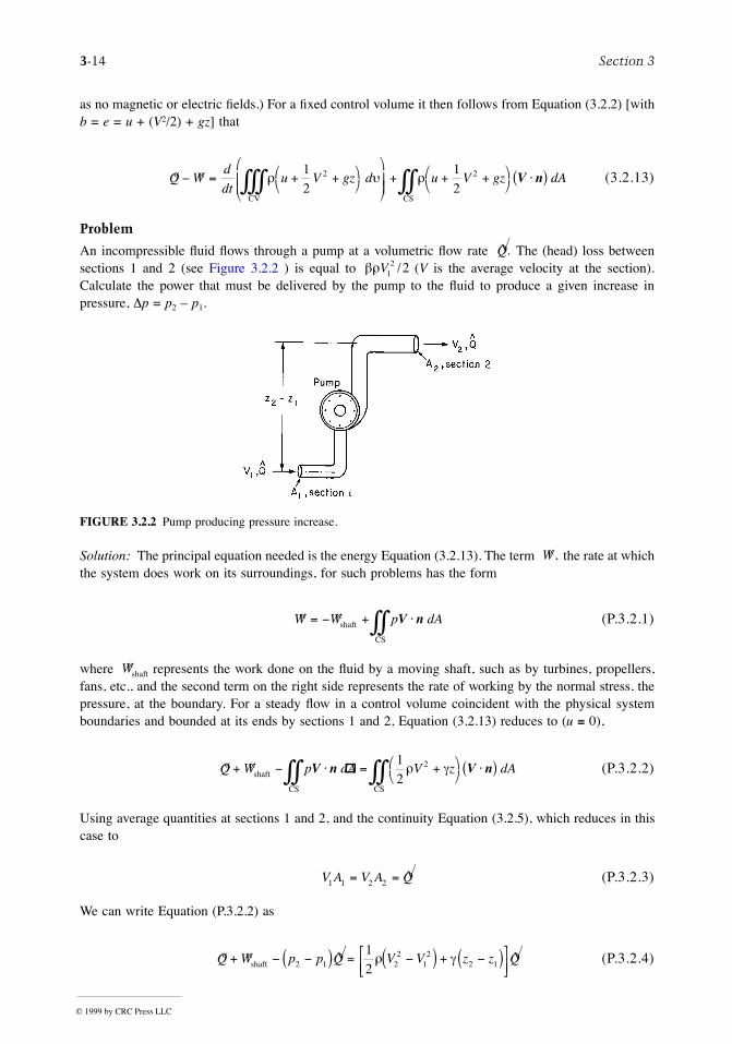
Problem
An incompressible ßuid ßows through a pump at a volumetric ßow rate The (head) loss betweensections 1 and 2 (see Figure 3.2.2 ) is equal to (V is the average velocity at the section).Calculate the power that must be delivered by the pump to the ßuid to produce a given increase inpressure, Dp = p2 Ð p1.
Solution: The principal equation needed is the energy Equation (3.2.13). The term the rate at whichthe system does work on its surroundings, for such problems has the form
(P.3.2.1)
where represents the work done on the ßuid by a moving shaft, such as by turbines, propellers,fans, etc., and the second term on the right side represents the rate of working by the normal stress, thepressure, at the boundary. For a steady ßow in a control volume coincident with the physical systemboundaries and bounded at its ends by sections 1 and 2, Equation (3.2.13) reduces to (u º 0),
(P.3.2.2)
Using average quantities at sections 1 and 2, and the continuity Equation (3.2.5), which reduces in thiscase to
(P.3.2.3)
We can write Equation (P.3.2.2) as
(P.3.2.4)
FIGURE 3.2.2 Pump producing pressure increase.
Ç ÇQ Wd
dtu V gz d u V gz dA- = + +æ
èöø
æ
èçç
ö
ø÷÷
+ + +æè
öø
×( )òòò òòr u r12
12
2 2
CV CS
V n
Ã.QbrV1
2 2/
Ç,W
Ç ÇW W p dA= - + ×òòshaft
CS
V n
ÇWshaft
Ç ÇQ W p dA V z dA+ - × = +æè
öø
×( )òò òòshaft
CS CS
V n V n12
2r g
V A V A Q1 1 2 2= = Ã
Ç Ç Ã ÃQ W p p Q V V z z Q+ - -( ) = -( ) + -( )éëê
ùûúshaft 2 1 2
212
2 1
12
r g
© 1999 by CRC Press LLC
Fluid Mechanics 3-15
the rate at which heat is added to the system, is here equal to Ð the head loss betweensections 1 and 2. Equation (P.3.2.4) then can be rewritten
or, in terms of the given quantities,
(P.3.2.5)
Thus, for example, if the ßuid is water (r » 1000 kg/m3, g = 9.8 kN/m3), = 0.5 m3/sec, the heatloss is and Dp = p2 Ð p1 = 2 ´ 105N/m2 = 200 kPa, A1 = 0.1 m2 = A2/2, (z2 Ð z1) = 2 m, weÞnd, using Equation (P.3.2.5)
Differential Relations for Fluid Motion
In the previous section the conservation laws were derived in integral form. These forms are useful incalculating, generally using a control volume analysis, gross features of a ßow. Such analyses usuallyrequire some a priori knowledge or assumptions about the ßow. In any case, an approach based onintegral conservation laws cannot be used to determine the point-by-point variation of the dependentvariables, such as velocity, pressure, temperature, etc. To do this requires the use of the differential formsof the conservation laws, which are presented below.
Mass Conservation–Continuity Equation
Applying GaussÕs theorem (the divergence theorem) to Equation (3.2.3) we obtain
(3.2.14)
which, because the control volume is arbitrary, immediately yields
(3.2.15)
This can also be written as
(3.2.16)
Ç,Q brV12 2/ ,
Ç Ã Ã ÃWV
p Q V V Q z z Qshaft = + ( ) + -( ) + -( )br r g12
22
12
2 1212
D
ÇÃ
ÃÃ
ÃWQ
Ap Q
Q
A
A
Az z Qshaft = + ( ) + -
æ
èç
ö
ø÷ + -( )br
r g2
12
3
22
22
12 2 1
12
1D
ÃQ0 2 21
2. / ,rV
Ç . .
..
.
.. .
, , , , ,
,,
.
Wshaft
Nm sec
W hp hp
=( )( )
( )+ ´( )( ) + ( ) ( )
( )-( ) + ´( )( )( )
= + - + =
= = =
0 2 1000 0 5
0 12 10 0 5
12
10000 5
0 21 4 9 8 10 2 0 5
5 000 10 000 4 688 9 800 20 112
20 11220 112745 7
27
2
25
3
23
¶r
r ut
d+ Ñ × ( )é
ëêù
ûú=
( )
òòò VCV
fixed
0
¶r
rt
+ Ñ × ( ) =V 0
D
Dt
rr+ Ñ × =V 0
© 1999 by CRC Press LLC
3-16 Section 3
using the fact that
(3.2.17)
Special cases:
1. Steady ßow [(¶/¶t) ( ) º 0]
(3.2.18)
2. Incompressible ßow (Dr/Dt º 0)
(3.2.19)
Momentum Conservation
We note Þrst, as a consequence of mass conservation for a system, that the right-hand side of Equation(3.2.6) can be written as
(3.2.20)
The total force acting on the system which appears on the left-hand side of Equation (3.2.6) is the sumof body forces Fb and surface forces Fs. The body forces are often given as forces per unit mass (e.g.,gravity), and so can be written
(3.2.21)
The surface forces are represented in terms of the second-order stress tensor* = {sij}, where sij isdeÞned as the force per unit area in the i direction on a planar element whose normal lies in the jdirection. From elementary angular momentum considerations for an inÞnitesimal volume it can beshown that sij is a symmetric tensor, and therefore has only six independent components. The totalsurface force exerted on the system by its surroundings is then
(3.2.22)
The integral momentum conservation law Equation (3.2.6) can then be written
(3.2.23)
* We shall assume the reader is familiar with elementary Cartesian tensor analysis and the associated subscriptnotation and conventions. The reader for whom this is not true should skip the details and concentrate on the Þnalprincipal results and equations given at the ends of the next few subsections.
D
Dt t
r ¶r
r= + × ÑV
Ñ × ( ) =rV 0
Ñ × =V 0
D
Dtd
D
Dtdr u r uV
V
system systemòòò òòò
æ
èçç
ö
ø÷÷
º
F fb d= òòòr usystem
s
F ns s ij jdA i F n dAi
= × - =òò òòs ssystemsurface
with component,
r u r u sD
Dtd d dA
Vf n
system system systemsurface
òòò òòò òò= + ×
© 1999 by CRC Press LLC
Fluid Mechanics 3-17
The application of the divergence theorem to the last term on the right-side of Equation (3.2.23) leads to
(3.2.24)
where Ñ á º {¶sij/xj}. Since Equation (3.2.24) holds for any material volume, it follows that
(3.2.25)
(With the decomposition of Ftotal above, Equation (3.2.10) can be written
(3.2.26)
If r is uniform and f is a conservative body force, i.e., f = ÐÑY, where Y is the force potential, thenEquation (3.2.26), after application of the divergence theorem to the body force term, can be written
(3.2.27)
It is in this form, involving only integrals over the surface of the control volume, that the integral formof the momentum equation is used in control volume analyses, particularly in the case when the bodyforce term is absent.)
Analysis of Rate of Deformation
The principal aim of the following two subsections is to derive a relationship between the stress and therate of strain to be used in the momentum Equation (3.2.25). The reader less familiar with tensor notationmay skip these sections, apart from noting some of the terms and quantities deÞned therein, and proceeddirectly to Equations (3.2.38) or (3.2.39).
The relative motion of two neighboring points P and Q, separated by a distance h, can be written(using u for the local velocity)
or, equivalently, writing Ñu as the sum of antisymmetric and symmetric tensors,
(3.2.28)
where Ñu = {¶ui/¶xj}, and the superscript * denotes transpose, so (Ñu)* = {¶uj/¶xi}. The second termon the right-hand side of Equation (3.2.28) can be rewritten in terms of the vorticity, Ñ ´ u, so Equation(3.2.28) becomes
(3.2.29)
r u r u s uD
Dtd d d
Vf
system system systemòòò òòò òòò= + Ñ ×
s
r r sD
Dt
Vf= + Ñ ×
r u s rf n V V nd dA dA
CV CS CSòòò òò òò+ × = ×( )
- + ×( ) = ×( )òò òòr s rYn n V V ndA dA
CS CS
u u uQ P( ) = ( ) + Ñ( )h
u u u u u uQ P( ) = ( ) + Ñ( ) - Ñ( )( ) + Ñ( ) + Ñ( )( )12
12
* *h h
u u u u uQ P( ) = ( ) + Ñ ´( ) ´ + Ñ( ) + Ñ( )( )12
12
h h*
© 1999 by CRC Press LLC
3-18 Section 3
which shows that the local rate of deformation consists of a rigid-body translation, a rigid-body rotationwith angular velocity 1/2 (Ñ ´ u), and a velocity or rate of deformation. The coefÞcient of h in the lastterm in Equation (3.2.29) is deÞned as the rate-of-strain tensor and is denoted by , in subscript form
(3.2.30)
From we can deÞne a rate-of-strain central quadric, along the principal axes of which the deformingmotion consists of a pure extension or compression.
Relationship Between Forces and Rate of Deformation
We are now in a position to determine the required relationship between the stress tensor and therate of deformation. Assuming that in a static ßuid the stress reduces to a (negative) hydrostatic orthermodynamic pressure, equal in all directions, we can write
(3.2.31)
where is the viscous part of the total stress and is called the deviatoric stress tensor, is the identitytensor, and dij is the corresponding Kronecker delta (dij = 0 if i ¹ j; dij = 1 if i = j). We make furtherassumptions that (1) the ßuid exhibits no preferred directions; (2) the stress is independent of any previoushistory of distortion; and (3) that the stress depends only on the local thermodynamic state and thekinematic state of the immediate neighborhood. Precisely, we assume that is linearly proportional tothe Þrst spatial derivatives of u, the coefÞcient of proportionality depending only on the local thermo-dynamic state. These assumptions and the relations below which follow from them are appropriate fora Newtonian ßuid. Most common ßuids, such as air and water under most conditions, are Newtonian,but there are many other ßuids, including many which arise in industrial applications, which exhibit so-called non-Newtonian properties. The study of such non-Newtonian ßuids, such as viscoelastic ßuids,is the subject of the Þeld of rheology.
With the Newtonian ßuid assumptions above, and the symmetry of which follows from thesymmetry of , one can show that the viscous part of the total stress can be written as
(3.2.32)
so the total stress for a Newtonian ßuid is
(3.2.33)
or, in subscript notation
(3.2.34)
(the Einstein summation convention is assumed here, namely, that a repeated subscript, such as in thesecond term on the right-hand side above, is summed over; note also that Ñ á u = ¶uk/¶xk = ekk.) ThecoefÞcient l is called the Òsecond viscosityÓ and m the Òabsolute viscosity,Ó or more commonly theÒdynamic viscosity,Ó or simply the Òviscosity.Ó For a Newtonian ßuid l and m depend only on localthermodynamic state, primarily on the temperature.
e
eu
x
u
xiji
j
j
i
= +æ
èç
ö
ø÷
12
e
s
s t s d t= - + = - +pI pij ij ijor
t I
t
ts t
t l m= Ñ ×( ) +u I e2
s l m= - + Ñ ×( ) +pI I eu 2
s d l
¶d m
¶ij ijk
kij
i
j
j
i
pu
x
u
x
u
x= - +
æ
èç
ö
ø÷ + +
æ
èç
ö
ø÷
© 1999 by CRC Press LLC
Fluid Mechanics 3-19
We note, from Equation (3.2.34), that whereas in a ßuid at rest the pressure is an isotropic normalstress, this is not the case for a moving ßuid, since in general s11 ¹ s22 ¹ s33. To have an analogousquantity to p for a moving ßuid we deÞne the pressure in a moving ßuid as the negative mean normalstress, denoted, say, by
(3.2.35)
(sii is the trace of and an invariant of , independent of the orientation of the axes). From Equation(3.2.34)
(3.2.36)
For an incompressible ßuid Ñ á u = 0 and hence º p. The quantity (l + 2/3m) is called the bulkviscosity. If one assumes that the deviatoric stress tensor tij makes no contribution to the mean normalstress, it follows that l + 2/3m = 0, so again = p. This condition, l = Ð2/3m, is called the Stokesassumption or hypothesis. If neither the incompressibility nor the Stokes assumptions are made, thedifference between and p is usually still negligibly small because (l + 2/3m) Ñ á u << p in most ßuidßow problems. If the Stokes hypothesis is made, as is often the case in ßuid mechanics, Equation (3.2.34)becomes
(3.2.37)
The Navier–Stokes Equations
Substitution of Equation (3.2.33) into (3.2.25), since Ñ á = Ñf, for any scalar function f, yields(replacing u in Equation (3.2.33) by V)
(3.2.38)
These equations are the NavierÐStokes equations (although the name is as often given to the full set ofgoverning conservation equations). With the Stokes assumption (l = Ð2/3m), Equation (3.2.38) becomes
(3.2.39)
If the Eulerian frame is not an inertial frame, then one must use the transformation to an inertial frameeither using Equation (3.2.8) or the ÒapparentÓ body force formulation, Equation (3.2.9).
Energy Conservation — The Mechanical and Thermal Energy Equations
In deriving the differential form of the energy equation we begin by assuming that heat enters or leavesthe material or control volume by heat conduction across the boundaries, the heat ßux per unit areabeing q. It then follows that
(3.2.40)
p
p ii= -13
s
s s
p pii= - = - +æè
öøÑ ×
13
23
s l m u
p
p
p
s d m dij ij ij kk ijp e e= - + -æè
öø
213
( )fI
r r l mD
Dtp e
Vf V= - Ñ + Ñ Ñ ×( ) + Ñ × ( )2
r r mD
Dtp e e Ikk
Vf= - Ñ + Ñ × -æ
èöø
é
ëê
ù
ûú2
13
ÇQ dA d= - × = - Ñ ×òò òòòq n q u
© 1999 by CRC Press LLC
3-20 Section 3
The work-rate term can be decomposed into the rate of work done against body forces, given by
Ð (3.2.41)
and the rate of work done against surface stresses, given by
(3.2.42)
Substitution of these expressions for and into Equation (3.2.12), use of the divergence theorem,and conservation of mass lead to
(3.2.43)
(note that a potential energy term is no longer included in e, the total speciÞc energy, as it is accountedfor by the body force rate-of-working term rf á V).
Equation (3.2.43) is the total energy equation showing how the energy changes as a result of workingby the body and surface forces and heat transfer. It is often useful to have a purely thermal energyequation. This is obtained by subtracting from Equation (3.2.43) the dot product of V with the momentumEquation (3.2.25), after expanding the last term in Equation (3.2.43), resulting in
(3.2.44)
With sij = Ðpdij + tij, and the use of the continuity equation in the form of Equation (3.2.16), the Þrstterm on the right-hand side of Equation (3.2.44) may be written
(3.2.45)
where F is the rate of dissipation of mechanical energy per unit mass due to viscosity, and is given by
(3.2.46)
With the introduction of Equation (3.2.45), Equation (3.2.44) becomes
(3.2.47)
or
(3.2.48)
ÇW
r uf Vòòò × d
- × ( )òòV nsystemsurface
s dA
ÇQ ÇW
r r sD
Dtu V+æ
èöø
= -Ñ × + × + Ñ × ( )12
2 q f V V
r
¶s
Du
Dt
V
xi
jij= - Ñ × q
¶s r
rV
x
Dp
Dt
Dp
Dti
jij = -
æ
èç
ö
ø÷
+ + F
F º = -æè
öø
= -æè
öø
¶t m m d
V
xe e e e ei
jij ij ij kk ij kk ij2
13
213
22
rDe
Dtp= - Ñ × + - Ñ ×V qF
rDh
Dt
Dp
Dt= + - Ñ ×F q
© 1999 by CRC Press LLC
Fluid Mechanics 3-21
where h = e + (p/r) is the speciÞc enthalpy. Unlike the other terms on the right-hand side of Equation(3.2.47), which can be negative or positive, F is always nonnegative and represents the increase ininternal energy (or enthalpy) owing to irreversible degradation of mechanical energy. Finally, fromelementary thermodynamic considerations
where S is the entropy, so Equation (3.2.48) can be written
(3.2.49)
If the heat conduction is assumed to obey the Fourier heat conduction law, so q = Ð kÑT, where k is thethermal conductivity, then in all of the above equations
(3.2.50)
the last of these equalities holding only if k = constant.In the event the thermodynamic quantities vary little, the coefÞcients of the constitutive relations for and q may be taken to be constant and the above equations simpliÞed accordingly.We note also that if the ßow is incompressible, then the mass conservation, or continuity, equation
simpliÞes to
(3.2.51)
and the momentum Equation (3.2.38) to
(3.2.52)
where Ñ2 is the Laplacian operator. The small temperature changes, compatible with the incompressibilityassumption, are then determined, for a perfect gas with constant k and speciÞc heats, by the energyequation rewritten for the temperature, in the form
(3.2.53)
Boundary Conditions
The appropriate boundary conditions to be applied at the boundary of a ßuid in contact with anothermedium depends on the nature of this other medium Ñ solid, liquid, or gas. We discuss a few of themore important cases here in turn:
1. At a solid surface: V and T are continuous. Contained in this boundary condition is the Òno-slipÓcondition, namely, that the tangential velocity of the ßuid in contact with the boundary of thesolid is equal to that of the boundary. For an inviscid ßuid the no-slip condition does not apply,and only the normal component of velocity is continuous. If the wall is permeable, the tangentialvelocity is continuous and the normal velocity is arbitrary; the temperature boundary conditionfor this case depends on the nature of the injection or suction at the wall.
Dh
DtT
DS
Dt
Dp
Dt= +
1r
rTDS
Dt= - Ñ ×F q
- Ñ × = Ñ × Ñ( ) = Ñq k T k T2
s
Ñ × =V 0
r r mD
Dtp
Vf V= - Ñ + Ñ2
rcvDT
Dtk T= Ñ +2 F
© 1999 by CRC Press LLC
3-22 Section 3
2. At a liquid/gas interface: For such cases the appropriate boundary conditions depend on whatcan be assumed about the gas the liquid is in contact with. In the classical liquid free-surfaceproblem, the gas, generally atmospheric air, can be ignored and the necessary boundary conditionsare that (a) the normal velocity in the liquid at the interface is equal to the normal velocity of theinterface and (b) the pressure in the liquid at the interface exceeds the atmospheric pressure byan amount equal to
(3.2.54)
where R1 and R2 are the radii of curvature of the intercepts of the interface by two orthogonalplanes containing the vertical axis. If the gas is a vapor which undergoes nonnegligible interactionand exchanges with the liquid in contact with it, the boundary conditions are more complex. Then,in addition to the above conditions on normal velocity and pressure, the shear stress (momentumßux) and heat ßux must be continuous as well.
For interfaces in general the boundary conditions are derived from continuity conditions for eachÒtransportableÓ quantity, namely continuity of the appropriate intensity across the interface and continuityof the normal component of the ßux vector. Fluid momentum and heat are two such transportablequantities, the associated intensities are velocity and temperature, and the associated ßux vectors arestress and heat ßux. (The reader should be aware of circumstances where these simple criteria do notapply, for example, the velocity slip and temperature jump for a rareÞed gas in contact with a solidsurface.)
Vorticity in Incompressible Flow
With m = constant, r = constant, and f = Ðg = Ðgk the momentum equation reduces to the form (seeEquation (3.2.52))
(3.2.55)
With the vector identities
(3.2.56)
and
(3.2.57)
and deÞning the vorticity
(3.2.58)
Equation (3.2.55) can be written, noting that for incompressible ßow Ñ á V = 0,
(3.2.59)
Dp p pR R
= - = +æ
èç
ö
ø÷liquid atm s
1 1
1 2
r r mD
Dtp g
Vk V= -Ñ - + Ñ2
V V V V× Ñ( ) = Ñæ
èç
ö
ø÷ - ´ Ñ ´( )V 2
2
Ñ = Ñ Ñ ×( ) - Ñ ´ Ñ ´( )2V V V
zz º Ñ ´ V
r¶¶
r r r mV
Vt
p V gz+ Ñ + +æè
öø
= ´ - Ñ ´12
2 zz zz
© 1999 by CRC Press LLC
Fluid Mechanics 3-23
The ßow is said to be irrotational if
(3.2.60)
from which it follows that a velocity potential F can be deÞned
(3.2.61)
Setting z = 0 in Equation (3.2.59), using Equation (3.2.61), and then integrating with respect to all thespatial variables, leads to
(3.2.62)
(the arbitrary function F(t) introduced by the integration can either be absorbed in F, or is determinedby the boundary conditions). Equation (3.2.62) is the unsteady Bernoulli equation for irrotational,incompressible ßow. (Irrotational ßows are always potential ßows, even if the ßow is compressible.Because the viscous term in Equation (3.2.59) vanishes identically for z = 0, it would appear that theabove Bernoulli equation is valid even for viscous ßow. Potential solutions of hydrodynamics are in factexact solutions of the full NavierÐStokes equations. Such solutions, however, are not valid near solidboundaries or bodies because the no-slip condition generates vorticity and causes nonzero z; the potentialßow solution is invalid in all those parts of the ßow Þeld that have been ÒcontaminatedÓ by the spreadof the vorticity by convection and diffusion. See below.)
The curl of Equation (3.2.59), noting that the curl of any gradient is zero, leads to
(3.2.63)
but
(3.2.64)
since div curl ( ) º 0, and therefore also
(3.2.65)
(3.2.66)
Equation (3.2.63) can then be written
(3.2.67)
where n = m/r is the kinematic viscosity. Equation (3.2.67) is the vorticity equation for incompressibleßow. The Þrst term on the right, an inviscid term, increases the vorticity by vortex stretching. In inviscid,two-dimensional ßow both terms on the right-hand side of Equation (3.2.67) vanish, and the equationreduces to Dz/Dt = 0, from which it follows that the vorticity of a ßuid particle remains constant as itmoves. This is HelmholtzÕs theorem. As a consequence it also follows that if z = 0 initially, z º 0 always;
zz º Ñ ´ =V 0
V = ÑF
r¶¶
r rFt
p V gz F t+ + +æè
öø
= ( )12
2
r¶¶
r mzz
zz zzt
= Ñ ´ ´( ) - Ñ ´ Ñ ´V
Ñ = Ñ Ñ ×( ) - Ñ ´ Ñ ´
= -Ñ ´ Ñ ´
2zz zz zz
zz
Ñ ´ ´( ) º Ñ( ) + Ñ × - Ñ - Ñ ×V V V V Vzz zz zz zz zz
= Ñ( ) - Ñzz zzV V
D
Dt
zzzz zz= × Ñ( ) + ÑV n 2
© 1999 by CRC Press LLC
3-24 Section 3
i.e., initially irrotational ßows remain irrotational (for inviscid ßow). Similarly, it can be proved thatDG/Dt = 0; i.e., the circulation around a material closed circuit remains constant, which is KelvinÕstheorem.
If n ¹ 0, Equation (3.2.67) shows that the vorticity generated, say, at solid boundaries, diffuses andstretches as it is convected.
We also note that for steady ßow the Bernoulli equation reduces to
(3.2.68)
valid for steady, irrotational, incompressible ßow.
Stream Function
For two-dimensional ßows the continuity equation, e.g., for plane, incompressible ßows (V = (u, n))
(3.2.69)
can be identically satisÞed by introducing a stream function y, deÞned by
(3.2.70)
Physically y is a measure of the ßow between streamlines. (Stream functions can be similarly deÞnedto satisfy identically the continuity equations for incompressible cylindrical and spherical axisymmetricßows; and for these ßows, as well as the above planar ßow, also when they are compressible, but onlythen if they are steady.) Continuing with the planar case, we note that in such ßows there is only a singlenonzero component of vorticity, given by
(3.2.71)
With Equation (3.2.70)
(3.2.72)
For this two-dimensional ßow Equation (3.2.67) reduces to
(3.2.73)
Substitution of Equation (3.2.72) into Equation (3.2.73) yields an equation for the stream function
(3.2.74)
p V gz+ + =12
2r r constant
¶¶
¶n
u
x y+ = 0
uy x
= = -¶y
n¶y
,
zz = ( ) = -æ
èç
ö
ø÷0 0 0 0, , , ,z
¶n
¶¶z x
u
y
z¶ y
¶ y
yz x y= - - = -Ñ
2
2
2
22
¶z
¶z
¶n
¶z
¶n
¶ z
¶ z
¶z z z z z
tu
x y x y+ + = +
æ
èç
ö
ø÷
2
2
2
2
¶ y
¶¶y
¶ y
¶¶y
¶¶
y n yÑ( )
+Ñ( )
- Ñ( ) = Ñ2 2
2 4
t y x x y
© 1999 by CRC Press LLC
Fluid Mechanics 3-25
where Ñ4 = Ñ2 (Ñ2). For uniform ßow past a solid body, for example, this equation for Y would besolved subject to the boundary conditions:
(3.2.75)
For the special case of irrotational ßow it follows immediately from Equations (3.2.70) and (3.2.71)with zz = 0, that y satisÞes the Laplace equation
(3.2.76)
Inviscid Irrotational Flow: Potential Flow
For irrotational ßows we have already noted that a velocity potential F can be deÞned such that V =ÑF. If the flow is also incompressible, so Ñ á V = 0, it then follows that
(3.2.77)
so F satisÞes LaplaceÕs equation. (Note that unlike the stream function y, which can only be deÞnedfor two-dimensional ßows, the above considerations for F apply to ßow in two and three dimensions.On the other hand, the existence of y does not require the ßow to be irrotational, whereas the existenceof F does.)
Since Equation (3.2.77) with appropriate conditions on V at boundaries of the ßow completelydetermines the velocity Þeld, and the momentum equation has played no role in this determination, wesee that inviscid irrotational ßow Ñ potential theory Ñ is a purely kinematic theory. The momentumequation only enters after F is known in order to calculate the pressure Þeld consistent with the velocityÞeld V = ÑF.
For both two- and three-dimensional ßows the determination of F makes use of the powerful tech-niques of potential theory, well developed in the mathematical literature. For two-dimensional planarßows the techniques of complex variable theory are available, since F may be considered as either thereal or imaginary part of an analytic function (the same being true for y, since for such two-dimensionalßows F and y are conjugate variables.)
Because the Laplace equation, obeyed by both F and y, is linear, complex ßows may be built upfrom the superposition of simple ßows; this property of inviscid irrotational ßows underlies nearly allsolution techniques in this area of ßuid mechanics.
Problem
A two-dimensional inviscid irrotational ßow has the velocity potential
(P.3.2.6)
What two-dimensional potential ßow does this represent?
Solution. It follows from Equations (3.2.61) and (3.2.70) that for two-dimensional ßows, in general
(P.3.2.7)
¶y
¶y
¶y
¶y
x yV
x y
= =
= = ( )
¥0
0 0
,
,
at infinity
at the body no-slip
Ñ = + =22
2
2
2 0y¶ y
¶ y¶x y
Ñ × Ñ( ) = Ñ =F F2 0
F = -x y2 2
ux y y x
= = = = -¶¶
¶y
n¶¶
¶y
F F,
© 1999 by CRC Press LLC
3-26 Section 3
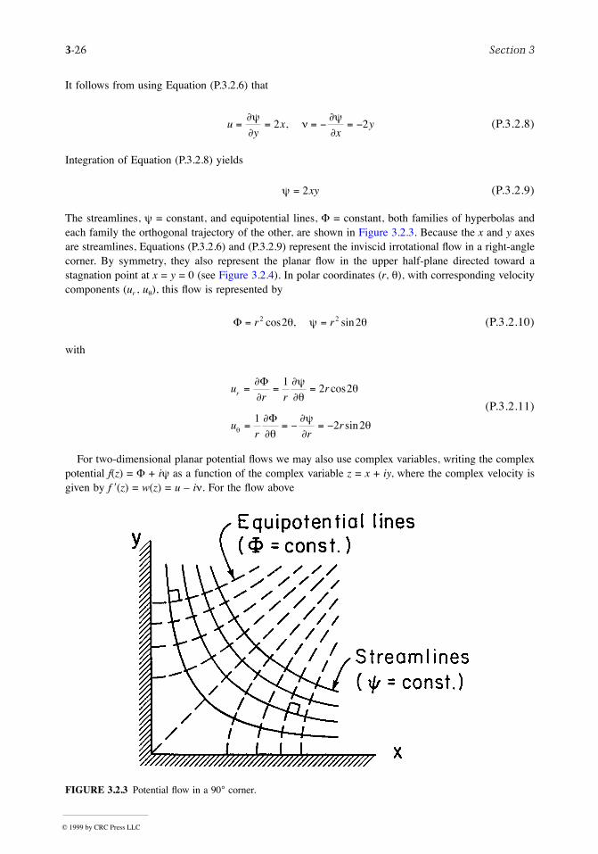
It follows from using Equation (P.3.2.6) that
(P.3.2.8)
Integration of Equation (P.3.2.8) yields
(P.3.2.9)
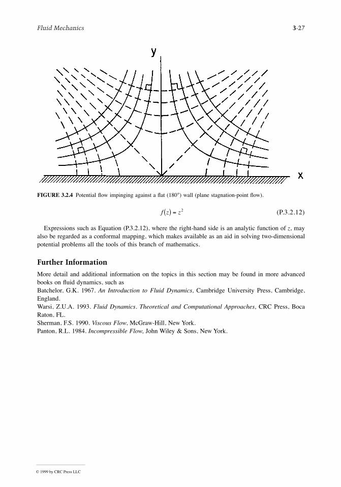
The streamlines, y = constant, and equipotential lines, F = constant, both families of hyperbolas andeach family the orthogonal trajectory of the other, are shown in Figure 3.2.3. Because the x and y axesare streamlines, Equations (P.3.2.6) and (P.3.2.9) represent the inviscid irrotational ßow in a right-anglecorner. By symmetry, they also represent the planar ßow in the upper half-plane directed toward astagnation point at x = y = 0 (see Figure 3.2.4). In polar coordinates (r, q), with corresponding velocitycomponents (ur , uq), this ßow is represented by
(P.3.2.10)
with
(P.3.2.11)
For two-dimensional planar potential ßows we may also use complex variables, writing the complexpotential f(z) = F + iy as a function of the complex variable z = x + iy, where the complex velocity isgiven by f ¢(z) = w(z) = u Ð in. For the ßow above
FIGURE 3.2.3 Potential ßow in a 90° corner.
uy
xx
y= = = - = -¶y
n¶y
2 2,
y = 2xy
F = =r r2 22 2cos , sinq y q
ur r
r
ur r
r
r = = =
= = - = -
¶¶
¶y¶q
q
¶¶q
¶y
F
F
12 2
12 2
cos
sin
© 1999 by CRC Press LLC
Fluid Mechanics 3-27
(P.3.2.12)
Expressions such as Equation (P.3.2.12), where the right-hand side is an analytic function of z, mayalso be regarded as a conformal mapping, which makes available as an aid in solving two-dimensionalpotential problems all the tools of this branch of mathematics.
Further Information
More detail and additional information on the topics in this section may be found in more advancedbooks on ßuid dynamics, such asBatchelor, G.K. 1967. An Introduction to Fluid Dynamics, Cambridge University Press, Cambridge,England.Warsi, Z.U.A. 1993. Fluid Dynamics. Theoretical and Computational Approaches, CRC Press, BocaRaton, FL.Sherman, F.S. 1990. Viscous Flow, McGraw-Hill, New York.Panton, R.L. 1984. Incompressible Flow, John Wiley & Sons, New York.
FIGURE 3.2.4 Potential ßow impinging against a ßat (180°) wall (plane stagnation-point ßow).
f z z( ) = 2
© 1999 by CRC Press LLC
3-28 Section 3
3.3 Similitude: Dimensional Analysis and Data Correlation
Stuart W. Churchill
Dimensional Analysis
Similitude refers to the formulation of a description for physical behavior that is general and independentof the individual dimensions, physical properties, forces, etc. In this subsection the treatment of similitudeis restricted to dimensional analysis; for a more general treatment see Zlokarnik (1991). The full powerand utility of dimensional analysis is often underestimated and underutilized by engineers. This techniquemay be applied to a complete mathematical model or to a simple listing of the variables that deÞne thebehavior. Only the latter application is described here. For a description of the application of dimensionalanalysis to a mathematical model see Hellums and Churchill (1964).
General Principles
Dimensional analysis is based on the principle that all additive or equated terms of a complete relationshipbetween the variables must have the same net dimensions. The analysis starts with the preparation of alist of the individual dimensional variables (dependent, independent, and parametric) that are presumedto deÞne the behavior of interest. The performance of dimensional analysis in this context is reasonablysimple and straightforward; the principal difÞculty and uncertainty arise from the identiÞcation of thevariables to be included or excluded. If one or more important variables are inadvertently omitted, thereduced description achieved by dimensional analysis will be incomplete and inadequate as a guide forthe correlation of a full range of experimental data or theoretical values. The familiar band of plottedvalues in many graphical correlations is more often a consequence of the omission of one or morevariables than of inaccurate measurements. If, on the other hand, one or more irrelevant or unimportantvariables are included in the listing, the consequently reduced description achieved by dimensionalanalysis will result in one or more unessential dimensionless groupings. Such excessive dimensionlessgroupings are generally less troublesome than missing ones because the redundancy will ordinarily berevealed by the process of correlation. Excessive groups may, however, suggest unnecessary experimentalwork or computations, or result in misleading correlations. For example, real experimental scatter mayinadvertently and incorrectly be correlated in all or in part with the variance of the excessive grouping.
In consideration of the inherent uncertainty in selecting the appropriate variables for dimensionalanalysis, it is recommended that this process be interpreted as a speculative and subject to correction ofthe basis of experimental data or other information. Speculation may also be utilized as a formal techniqueto identify the effect of eliminating a variable or of combining two or more. The latter aspect ofspeculation, which may be applied either to the original listing of dimensional variables or to the resultingset of dimensionless groups, is often of great utility in identifying possible limiting behavior or dimen-sionless groups of marginal signiÞcance. The systematic speculative elimination of all but the mostcertain variables, one at a time, followed by regrouping, is recommended as a general practice. Theadditional effort as compared with the original dimensional analysis is minimal, but the possible returnis very high. A general discussion of this process may be found in Churchill (1981).
The minimum number of independent dimensionless groups i required to describe the fundamentaland parametric behavior is (Buckingham, 1914)
(3.3.1)
where n is the number of variables and m is the number of fundamental dimensions such as mass M,length L, time q, and temperature T that are introduced by the variables. The inclusion of redundantdimensions such as force F and energy E that may be expressed in terms of mass, length, time, and
i n m= -
© 1999 by CRC Press LLC
Fluid Mechanics 3-29
temperature is at the expense of added complexity and is to be avoided. (Of course, mass could bereplaced by force or temperature by energy as alternative fundamental dimensions.) In some rare casesi is actually greater than n Ð m. Then
(3.3.2)
where k is the maximum number of the chosen variables that cannot be combined to form a dimensionlessgroup. Determination of the minimum number of dimensionless groups is helpful if the groups are tobe chosen by inspection, but is unessential if the algebraic procedure described below is utilized todetermine the groups themselves since the number is then obvious from the Þnal result.
The particular minimal set of dimensionless groups is arbitrary in the sense that two or more of thegroups may be multiplied together to any positive, negative, or fractional power as long as the numberof independent groups is unchanged. For example, if the result of a dimensional analysis is
(3.3.3)
where X, Y, and Z are independent dimensionless groups, an equally valid expression is
(3.3.4)
Dimensional analysis itself does not provide any insight as to the best choice of equivalent dimensionlessgroupings, such as between those of Equations (3.3.3) and (3.3.4). However, isolation of each of thevariables that are presumed to be the most important in a separate group may be convenient in terms ofinterpretation and correlation. Another possible criterion in choosing between alternative groupings maybe the relative invariance of a particular one. The functional relationship provided by Equation (3.3.3)may equally well be expressed as
(3.3.5)
where X is implied to be the dependent grouping and Y and Z to be independent or parametric groupings.Three primary methods of determining a minimal set of dimensionless variables are (1) by inspection;
(2) by combination of the residual variables, one at a time, with the set of chosen variables that cannotbe combined to obtain a dimensionless group; and (3) by an algebraic procedure. These methods areillustrated in the examples that follow.
Example 3.3.1: Fully Developed Flow of Water Through a Smooth Round Pipe
Choice of Variables. The shear stress tw on the wall of the pipe may be postulated to be a function ofthe density r and the dynamic viscosity m of the water, the inside diameter D of the pipe, and the space-mean of the time-mean velocity um. The limitation to fully developed ßow is equivalent to a postulateof independence from distance x in the direction of ßow, and the speciÞcation of a smooth pipe isequivalent to the postulate of independence from the roughness e of the wall. The choice of tw ratherthan the pressure drop per unit length ÐdP/dx avoids the need to include the acceleration due to gravityg and the elevation z as variables. The choice of um rather than the volumetric rate of ßow V, the massrate of ßow w, or the mass rate of ßow per unit area G is arbitrary but has some important consequencesas noted below. The postulated dependence may be expressed functionally as f{tw, r, m, D, um} = 0 ortw = f{r, m, D, um}.
i n k= -
f XY Z Y Z1 2 2 0, ,{ } =
f X Y Z, ,{ } = 0
X Y Z= { }f ,
© 1999 by CRC Press LLC
3-30 Section 3
Tabulation. Next prepare a tabular listing of the variables and their dimensions:
Minimal Number of Groups. The number of postulated variables is 5. Since the temperature does notoccur as a dimension for any of the variables, the number of fundamental dimensions is 3. From Equation(3.3.1), the minimal number of dimensionless groups is 5 Ð 3 = 2. From inspection of the above tabulation,a dimensionless group cannot be formed from as many as three variables such as D, m, and r. Hence,Equation (3.3.2) also indicates that i = 5 Ð 3 = 2.
Method of Inspection. By inspection of the tabulation or by trial and error it is evident that only twoindependent dimensionless groups may be formed. One such set is
Method of Combination. The residual variables tw and m may be combined in turn with the noncom-bining variables r, D, and um to obtain two groups such as those above.
Algebraic Method. The algebraic method makes formal use of the postulate that the functional relation-ship between the variables may in general be represented by a power series. In this example such apower series may be expressed as
where the coefÞcients Ai are dimensionless. Each additive term on the right-hand side of this expressionmust have the same net dimensions as tw. Hence, for the purposes of dimensional analysis, only the Þrstterm need be considered and the indexes may be dropped. The resulting highly restricted expression istw = ArambDc Substituting the dimensions for the variables gives
Equating the sum of the exponents of M, L, and q on the right-hand side of the above expression withthose of the left-hand side produces the following three simultaneous linear algebraic equations: 1 = a+ b; Ð1 = Ð3a Ð b + c + d; and Ð2 = Ðb Ð d, which may be solved for a, c, and d in terms of b to obtaina = 1 Ð b, c = Ðb, and d = 2 Ð b. Substitution then gives tw = Ar1-bmb DÐb which may be regrouped as
Since this expression is only the Þrst term of a power series, it should not be interpreted to imply that is necessarily proportional to some power at m/Dumr but instead only the equivalent of the
expression derived by the method of inspection. The inference of a power dependence between the
tw r m D um
M 1 1 1 0 0L Ð1 Ð3 Ð1 1 1q Ð2 0 Ð1 0 Ð1T 0 0 0 0 0
ft
r
r
mw
m
m
u
Du2 0,
ìíî
üýþ
=
t r mw ia b c
md
i
N
A D ui i i i==
å1
umd .
M
LA
M
L
M
LL
La bc
d
q q q2 3= æè
öø
æè
öø
æè
öø
umb2-
t
rm
rw
m m
b
uA
Du2 =æ
èç
ö
ø÷
t rw mu/ 2
© 1999 by CRC Press LLC
Fluid Mechanics 3-31
dimensionless groups is the most common and serious error in the use of the algebraic method ofdimensional analysis.
Speculative Reductions. Eliminating r as a variable on speculative grounds to
or its exact equivalent:
The latter expression with A = 8 is actually the exact solution for the laminar regime (Dumr/m < 1800).A relationship that does not include r may alternatively be derived directly from the solution by themethod of inspection as follows. First, r is eliminated from one group, say , by multiplying itwith Dumr/m to obtain
The remaining group containing r is now simply dropped. Had the original expression been composedof three independent groups each containing r, that variable would have to be eliminated from two ofthem before dropping the third one.
The relationships that are obtained by the speculative elimination of m, D, and um, one at a time, donot appear to have any range of physical validity. Furthermore, if w or G had been chosen as theindependent variable rather than um, the limited relationship for the laminar regime would not have beenobtained by the elimination of r.
Alternative Forms. The solution may also be expressed in an inÞnity of other forms such as
If tw is considered to be the principal dependent variable and um the principal independent variable, thislatter form is preferable in that these two quantities do not then appear in the same grouping. On theother hand, if D is considered to be the principal independent variable, the original formulation ispreferable. The variance of is less than that of twD/mum and twD2r/m2 in the turbulent regimewhile that of twD/mum is zero in the laminar regime. Such considerations may be important in devisingconvenient graphical correlations.
Alternative Notations. The several solutions above are more commonly expressed as
or
ft
mw
m
D
u
ìíî
üýþ
= 0
t
mw
m
D
uA=
t rw mu/ 2
ft
m
r
mw
m
mD
u
Du,
ìíî
üýþ
= 0
ft r
m
r
mw mD Du2
2 0,ìíî
üýþ
=
t rw mu/ 2
ff
20,Reì
íî
üýþ
=
ff Re
Re2
0,ìíî
üýþ
=
© 1999 by CRC Press LLC
3-32 Section 3
where f = 2 is the Fanning friction factor and Re = Dumr/m is the Reynolds number.The more detailed forms, however, are to be preferred for purposes of interpretation or correlation
because of the explicit appearance of the individual, physically measurable variables.
Addition of a Variable. The above results may readily be extended to incorporate the roughness e ofthe pipe as a variable. If two variables have the same dimensions, they will always appear as adimensionless group in the form of a ratio, in this case e appears most simply as e/D. Thus, the solutionbecomes
Surprisingly, as contrasted with the solution for a smooth pipe, the speculative elimination of m andhence of the group Dumr/m now results in a valid asymptote for Dumr/m ® ¥ and all Þnite values ofe/D, namely,
Example 3.3.2: Fully Developed Forced Convection in Fully Developed Flow in a Round Tube
It may be postulated for this process that h = f{D, um, r, m, k, cp}, where here h is the local heat transfercoefÞcient, and cp and k are the speciÞc heat capacity and thermal conductivity, respectively, of the ßuid.The corresponding tabulation is
The number of variables is 7 and the number of independent dimensions is 4, as is the number ofvariables such as D, um, r, and k that cannot be combined to obtain a dimensionless group. Hence, theminimal number of dimensionless groups is 7 Ð 4 = 3. The following acceptable set of dimensionlessgroups may be derived by any of the procedures illustrated in Example 1:
Speculative elimination of m results in
h D um r m k cp
M 1 0 0 1 1 1 0L 0 1 1 Ð3 Ð1 1 2q Ð3 0 Ð1 0 Ð1 Ð3 Ð2T Ð1 0 0 0 0 Ð1 Ð1
ff Re
Re2
20,
ìíî
üýþ
=
t rw mu/ 2
ft
r
r
mw
m
m
u
Du e
D2 0, ,ìíî
üýþ
=
ft
rw
mu
e
D2 0,ìíî
üýþ
=
hD
k
Du c
km p=
ìíî
üýþ
fr
m
m,
hD
k
Du c
km p=
ìíî
üýþ
fr
© 1999 by CRC Press LLC
Fluid Mechanics 3-33
which has often erroneously been inferred to be a valid asymptote for cpm/k ® 0. Speculative eliminationof D, um, r, k, and cp individually also does not appear to result in expressions with any physical validity.However, eliminating cp and r or um gives a valid result for the laminar regime, namely,
The general solutions for ßow and convection in a smooth pipe may be combined to obtain
which would have been obtained directly had um been replaced by tw in the original tabulation. Thislatter expression proves to be superior in terms of speculative reductions. Eliminating D results in
which may be expressed in the more conventional form of
where Nu = hD/k is the Nusselt number and Pr = cpm/k is the Prandtl number. This result appears to bea valid asymptote for Re ® ¥ and a good approximation for even moderate values (>5000) for largevalues of Pr. Elimination of m as well as D results in
or
which appears to be an approximate asymptote for Re ® ¥ and Pr ® 0. Elimination of both cp and ragain yields the appropriate result for laminar ßow, indicating that r rather than um is the meaningfulvariable to eliminate in this respect.
The numerical value of the coefÞcient A in the several expressions above depends on the mode ofheating, a true variable, but one from which the purely functional expressions are independent. If jw theheat ßux density at the wall, and Tw Ð Tm, the temperature difference between the wall and the bulk ofthe ßuid, were introduced as variables in place of h º jw/(Tw Ð Tm), another group such as cp(Tw Ð Tm)(Dr/m)2 or rcp(Tw Ð Tm)/tw or which represents the effect of viscous dissipation, wouldbe obtained. This effect is usually but not always negligible. (See Chapter 4.)
Example 3.3.3: Free Convection from a Vertical Isothermal Plate
The behavior for this process may be postulated to be represented by
hD
kA=
hD
k
D c
kw p=
ìíî
üýþ
ft r
m
m2
2 ,
h
k
c
kw
pm
t rf
m
( )=
ìíî
üýþ
1 2
Nu Re Pr= æè
öø { }f
2
1 2
f
h
cA
p wt r( )=1 2
Nu = RePrAf
2
1 2æè
öø
c T T up w m m( )/ ,- 2
h g T T x c kw p= -{ }¥f b m r, , , , , , ,
© 1999 by CRC Press LLC
3-34 Section 3
where g is the acceleration due to gravity, b is the volumetric coefÞcient of expansion with temperature,T¥ is the unperturbed temperature of the ßuid, and x is the vertical distance along the plate. Thecorresponding tabulation is
The minimal number of dimensionless groups indicated by both methods is 9 Ð 4 = 5. A satisfactoryset of dimensionless groups, as found by any of the methods illustrated in Example 1 is
It may be reasoned that the buoyant force which generates the convective motion must be proportionalto rgb(Tw Ð T¥), thus, g in the Þrst term on the right-hand side must be multiplied by b(Tw Ð T¥), resultingin
The effect of expansion other than on the buoyancy is now represented by b(Tw Ð T¥), and the effect ofviscous dissipation by cp(Tw Ð T¥)(rx/m)2. Both effects are negligible for all practical circumstances.Hence, this expression may be reduced to
or
where Nux = hx/k and Grx = r2gb(Tw Ð T¥)x3/m2 is the Grashof number.Elimination of x speculatively now results in
or
This expression appears to be a valid asymptote for Grx ® ¥ and a good approximation for the entireturbulent regime. Eliminating m speculatively rather than x results in
h g b Tw Ð T¥ x m r cp k
M 1 0 0 0 0 1 1 0 1L 0 1 0 0 1 Ð1 Ð3 2 1q Ð3 Ð2 0 0 0 Ð1 0 Ð2 Ð3T Ð1 0 Ð1 1 0 0 0 Ð1 1
hx
k
gx c
kT T c T T
xpw p w= -( ) -( )æ
èç
ö
ø÷
ìíï
îï
üýï
þï¥ ¥f
rm
mb
rm
2 3
2
2
, , ,
hx
k
g T T x c
kT T c T T
xw pw p w=
-( )-( ) -( )æ
èç
ö
ø÷
ìíï
îï
üýï
þï
¥¥ ¥f
r b
m
mb
rm
2 3
2
2
, , ,
hx
k
g T T x c
kw p=
-( )ìíï
îï
üýï
þï
¥fr b
m
m2 3
2 ,
Nu = Gr Prx xf ,{ }
hx
k
g T T xw=-( )æ
èç
ö
ø÷ { }¥r b
mf
2 3
2
1 3
Pr
Nu = Gr Prxx1 3f{ }
© 1999 by CRC Press LLC
Fluid Mechanics 3-35
or
The latter expression appears to be a valid asymptote for Pr ® 0 for all Grx, that is, for both the laminarand the turbulent regimes. The development of a valid asymptote for large values of Pr requires moresubtle reasoning. First cpm/k is rewritten as m/ra where a = k/rcp. Then r is eliminated speculativelyexcept as it occurs in rgb(Tw Ð T¥) and k/rcp. The result is
or
where
is the Rayleigh number. The expression appears to be a valid asymptote for Pr ® ¥ and a reasonableapproximation for even moderate values of Pr for all Grx, that is, for both the laminar and the turbulentregimes.
Eliminating x speculatively from the above expressions for small and large values of Pr results in
and
The former appears to be a valid asymptote for Pr ® 0 and Grx ® ¥ and a reasonable approximationfor very small values of Pr in the turbulent regime, while the latter is well conÞrmed as a valid asymptotefor Pr ® ¥ and Grx ® ¥ and as a good approximation for moderate and large values of Pr over theentire turbulent regime. The expressions in terms of Grx are somewhat more complicated than those interms of Rax, but are to be preferred since Grx is known to characterize the transition from laminar toturbulent motion in natural convection just as ReD does in forced ßow in a channel. The power ofspeculation combined with dimensional analysis is well demonstrated by this example in which validasymptotes are thereby attained for several regimes.
hx
k
c g T T x
kp w=
-( )ìíï
îï
üýï
þï
¥fr b2 2 3
2
Nu = Gr Prx xf 2{ }
hx
k
c g T T x
kp w=
-( )ìíï
îï
üýï
þï
¥fr b
m
2 3
Nu = Rax xf{ }
Ra Gr Prxp w
x
c g T T x
k=
-( )=¥r b
m
2 3
Nu = Gr Pr Ra Prx x xA A2 1 3 1 3( ) = ( )
Nu = Gr Pr Rax x xB B( ) = ( )1 3 1 3
© 1999 by CRC Press LLC
3-36 Section 3
Correlation of Experimental Data and Theoretical Values
Correlations of experimental data are generally developed in terms of dimensionless groups rather thanin terms of the separate dimensional variables in the interests of compactness and in the hope of greatergenerality. For example, a complete set of graphical correlations for the heat transfer coefÞcient h ofExample 3.3.2 above in terms of each of the six individual independent variables and physical propertiesmight approach book length, whereas the dimensionless groupings both imply that a single plot withone parameter should be sufÞcient. Furthermore, the reduced expression for the turbulent regime impliesthat a plot of Nu/Re f1/2 vs. Pr should demonstrate only a slight parametric dependence on Re or Re f1/2.Of course, the availability of a separate correlation for f as a function of Re is implied.
Theoretical values, that is, ones obtained by numerical solution of a mathematical model in terms ofeither dimensional variables or dimensionless groups, are presumably free from imprecision. Even so,because of their discrete form, the construction of a correlation or correlations for such values may beessential for the same reasons as for experimental data.
Graphical correlations have the merit of revealing general trends, of providing a basis for evaluationof the choice of coordinates, and most of all of displaying visually the scatter of the individual experi-mental values about a curve representing a correlation or their behavior on the mean. (As mentioned inthe previous subsection, the omission of a variable may give the false impression of experimental errorin such a plot.) On the other hand, correlating equations are far more convenient as an input to a computerthan is a graphical correlation. These two formats thus have distinct and complementary roles; bothshould generally be utilized. The merits and demerits of various graphical forms of correlations arediscussed in detail by Churchill (1979), while the use of logarithmic and arithmetic coordinates, theeffects of the appearance of a variable in both coordinates, and the effects of the distribution of errorbetween the dependent and independent variable are further illustrated by Wilkie (1985).
Churchill and Usagi (1972; 1974) proposed general usage of the following expression for the formu-lation of correlating equations:
(3.3.6)
where yo{x} and y¥{x} denote asymptotes for small and large values of x, respectively, and n is anarbitrary exponent. For convenience and simplicity, Equation (3.3.6) may be rearranged in either of thefollowing two forms:
(3.3.7)
or
(3.3.8)
where Y{x} º y{x}/yo{x} and Z{x} º y¥{x}/yo{x}. Equations (3.3.6), (3.3.7), and (3.3.9) are hereafterdenoted collectively as the CUE (ChurchillÐUsagi equation). The principle merits of the CUE as acanonical expression for correlation are its simple form, generality, and minimal degree of explicitempiricism, namely, only that of the exponent n, since the asymptotes yo{x} and y¥{x} are ordinarilyknown in advance from theoretical considerations or well-established correlations. Furthermore, as willbe shown, the CUE is quite insensitive to the numerical value of n. Although the CUE is itself verysimple in form, it is remarkably successful in representing closely very complex behavior, even includingthe dependence on secondary variables and parameters, by virtue of the introduction of such dependenciesthrough yo{x} and y¥{x}. In the rare instances in which such dependencies are not represented in theasymptotes, n may be correlated as a function of the secondary variables and/or parameters. Although
y x y x y xn n n{ } = { } + { }¥0
Y x Z xn n( )( ) = + { }1
Y x
Z x Z x
n
n
{ }{ }
æ
èç
ö
ø÷ = +
{ }1
1
© 1999 by CRC Press LLC
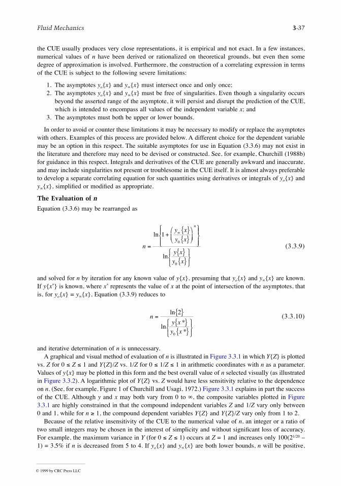
Fluid Mechanics 3-37
the CUE usually produces very close representations, it is empirical and not exact. In a few instances,numerical values of n have been derived or rationalized on theoretical grounds, but even then somedegree of approximation is involved. Furthermore, the construction of a correlating expression in termsof the CUE is subject to the following severe limitations:
1. The asymptotes yo{x} and y¥{x} must intersect once and only once;2. The asymptotes yo{x} and y¥{x} must be free of singularities. Even though a singularity occurs
beyond the asserted range of the asymptote, it will persist and disrupt the prediction of the CUE,which is intended to encompass all values of the independent variable x; and
3. The asymptotes must both be upper or lower bounds.
In order to avoid or counter these limitations it may be necessary to modify or replace the asymptoteswith others. Examples of this process are provided below. A different choice for the dependent variablemay be an option in this respect. The suitable asymptotes for use in Equation (3.3.6) may not exist inthe literature and therefore may need to be devised or constructed. See, for example, Churchill (1988b)for guidance in this respect. Integrals and derivatives of the CUE are generally awkward and inaccurate,and may include singularities not present or troublesome in the CUE itself. It is almost always preferableto develop a separate correlating equation for such quantities using derivatives or integrals of yo{x} andy¥{x}, simpliÞed or modiÞed as appropriate.
The Evaluation of n
Equation (3.3.6) may be rearranged as
(3.3.9)
and solved for n by iteration for any known value of y{x}, presuming that yo{x} and y¥{x} are known.If y{x*} is known, where x* represents the value of x at the point of intersection of the asymptotes, thatis, for yo{x} = y¥{x}, Equation (3.3.9) reduces to
(3.3.10)
and iterative determination of n is unnecessary.A graphical and visual method of evaluation of n is illustrated in Figure 3.3.1 in which Y{Z} is plotted
vs. Z for 0 £ Z £ 1 and Y{Z}/Z vs. 1/Z for 0 £ 1/Z £ 1 in arithmetic coordinates with n as a parameter.Values of y{x} may be plotted in this form and the best overall value of n selected visually (as illustratedin Figure 3.3.2). A logarithmic plot of Y{Z} vs. Z would have less sensitivity relative to the dependenceon n. (See, for example, Figure 1 of Churchill and Usagi, 1972.) Figure 3.3.1 explains in part the successof the CUE. Although y and x may both vary from 0 to ¥, the composite variables plotted in Figure3.3.1 are highly constrained in that the compound independent variables Z and 1/Z vary only between0 and 1, while for n ³ 1, the compound dependent variables Y{Z} and Y{Z}/Z vary only from 1 to 2.
Because of the relative insensitivity of the CUE to the numerical value of n, an integer or a ratio oftwo small integers may be chosen in the interest of simplicity and without signiÞcant loss of accuracy.For example, the maximum variance in Y (for 0 £ Z £ 1) occurs at Z = 1 and increases only 100(21/20 Ð1) = 3.5% if n is decreased from 5 to 4. If yo{x} and y¥{x} are both lower bounds, n will be positive,
n
y x
y x
y x
y x
n
=
+{ }{ }
æ
èç
ö
ø÷
ìíï
îï
üýï
þï
{ }{ }
ìíî
üýþ
¥ln
ln
10
0
ny x
y x
={ }{ }{ }
ìíî
üýþ
ln
ln*
*
2
0
© 1999 by CRC Press LLC
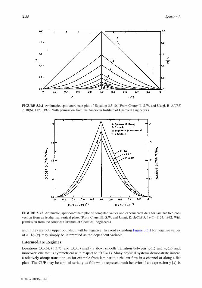
3-38 Section 3
and if they are both upper bounds, n will be negative. To avoid extending Figure 3.3.1 for negative valuesof n, 1/y{x} may simply be interpreted as the dependent variable.
Intermediate Regimes
Equations (3.3.6), (3.3.7), and (3.3.8) imply a slow, smooth transition between yo{x} and y¥{x} and,moreover, one that is symmetrical with respect to x*(Z = 1). Many physical systems demonstrate insteada relatively abrupt transition, as for example from laminar to turbulent ßow in a channel or along a ßatplate. The CUE may be applied serially as follows to represent such behavior if an expression yi{x} is
FIGURE 3.3.1 Arithmetic, split-coordinate plot of Equation 3.3.10. (From Churchill, S.W. and Usagi, R. AIChEJ. 18(6), 1123, 1972. With permission from the American Institute of Chemical Engineers.)
FIGURE 3.3.2 Arithmetic, split-coordinate plot of computed values and experimental data for laminar free con-vection from an isothermal vertical plate. (From Churchill, S.W. and Usagi, R. AIChE J. 18(6), 1124, 1972. Withpermission from the American Institute of Chemical Engineers.)
© 1999 by CRC Press LLC
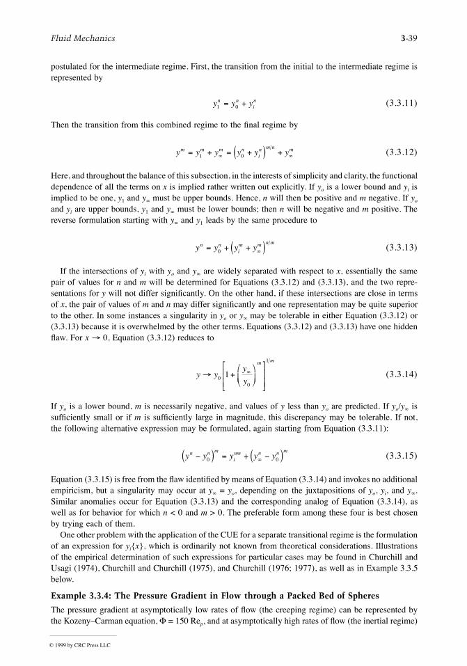
Fluid Mechanics 3-39
postulated for the intermediate regime. First, the transition from the initial to the intermediate regime isrepresented by
(3.3.11)
Then the transition from this combined regime to the Þnal regime by
(3.3.12)
Here, and throughout the balance of this subsection, in the interests of simplicity and clarity, the functionaldependence of all the terms on x is implied rather written out explicitly. If yo is a lower bound and yi isimplied to be one, y1 and y¥ must be upper bounds. Hence, n will then be positive and m negative. If yo
and yi are upper bounds, y1 and y¥ must be lower bounds; then n will be negative and m positive. Thereverse formulation starting with y¥ and y1 leads by the same procedure to
(3.3.13)
If the intersections of yi with yo and y¥ are widely separated with respect to x, essentially the samepair of values for n and m will be determined for Equations (3.3.12) and (3.3.13), and the two repre-sentations for y will not differ signiÞcantly. On the other hand, if these intersections are close in termsof x, the pair of values of m and n may differ signiÞcantly and one representation may be quite superiorto the other. In some instances a singularity in yo or y¥ may be tolerable in either Equation (3.3.12) or(3.3.13) because it is overwhelmed by the other terms. Equations (3.3.12) and (3.3.13) have one hiddenßaw. For x ® 0, Equation (3.3.12) reduces to
(3.3.14)
If yo is a lower bound, m is necessarily negative, and values of y less than yo are predicted. If yo/y¥ issufÞciently small or if m is sufÞciently large in magnitude, this discrepancy may be tolerable. If not,the following alternative expression may be formulated, again starting from Equation (3.3.11):
(3.3.15)
Equation (3.3.15) is free from the ßaw identiÞed by means of Equation (3.3.14) and invokes no additionalempiricism, but a singularity may occur at y¥ = yo, depending on the juxtapositions of yo, yi, and y¥.Similar anomalies occur for Equation (3.3.13) and the corresponding analog of Equation (3.3.14), aswell as for behavior for which n < 0 and m > 0. The preferable form among these four is best chosenby trying each of them.
One other problem with the application of the CUE for a separate transitional regime is the formulationof an expression for yi{x}, which is ordinarily not known from theoretical considerations. Illustrationsof the empirical determination of such expressions for particular cases may be found in Churchill andUsagi (1974), Churchill and Churchill (1975), and Churchill (1976; 1977), as well as in Example 3.3.5below.
Example 3.3.4: The Pressure Gradient in Flow through a Packed Bed of Spheres
The pressure gradient at asymptotically low rates of ßow (the creeping regime) can be represented bythe KozenyÐCarman equation, F = 150 Rep, and at asymptotically high rates of ßow (the inertial regime)
y y yn nin
1 0= +
y y y y y ym m m nin m n m= + = +( ) +¥ ¥1 0
y y y yn nim m n m
= + +( )¥0
y yy
y
m m
® +æ
èç
ö
ø÷
é
ë
êê
ù
û
úú
¥0
0
1
1
y y y y yn n m
inm n n m
-( ) = + -( )¥0 0
© 1999 by CRC Press LLC
3-40 Section 3
by the BurkeÐPlummer equation, F = 1.75 (Rep)2, where F = re2dp(ÐdPf /dx)m2(1 Ð e), Rep = dpuor/m(1Ð e), dp = diameter of spherical particles, m, e = void fraction of bed of spheres, dPf /dx = dynamicpressure gradient (due to friction), Pa/m, and uo = superÞcial velocity (in absence of the spheres), m/sec.For the origin of these two asymptotic expressions see Churchill (1988a). They both have a theoreticalstructure, but the numerical coefÞcients of 150 and 1.75 are basically empirical. These equations areboth lower bounds and have one intersection. Experimental data are plotted in Figure 3.3.3, which hasthe form of Figure 3.3.1 with Y = F/150 Rep, Y/Z = F/(1.75 Rep)2 and Z = 1.75 Rep = Rep/85.7.A value of n = 1 is seen to represent these data reasonably well on the mean, resulting in
which was originally proposed as a correlating equation by Ergun (1952) on the conjecture that thevolumetric fraction of the bed in ÒturbulentÓ ßow is proportional to Rep. The success of this expressionin conventional coordinates is shown in Figure 3.3.4. The scatter, which is quite evident in the arithmeticsplit coordinates of Figure 3.3.3, is strongly suppressed in a visual sense in the logarithmic coordinatesof Figure 3.3.4.
Example 3.3.5: The Friction Factor for Commercial Pipes for All Conditions
The serial application of the CUE is illustrated here by the construction of a correlating equation forboth smooth and rough pipes in the turbulent regime followed by combination of that expression withones for the laminar and transitional regimes.
The Turbulent Regime. The Fanning friction factor, fF, for turbulent ßow in a smooth round pipe forasymptotically large rates of ßow (say ReD > 5000) may be represented closely by the empiricalexpression:
FIGURE 3.3.3 Arithmetic, split-coordinate plot of experimental data for the pressure drop in ßow through a packedbed of spheres. (From Churchill, S.W. and Usagi, R. AIChE J. 18(6), 1123, 1972. With permission from the AmericanInstitute of Chemical Engineers.)
Re /p2 150
F = + ( )150 1 752
Re Rep p.
© 1999 by CRC Press LLC
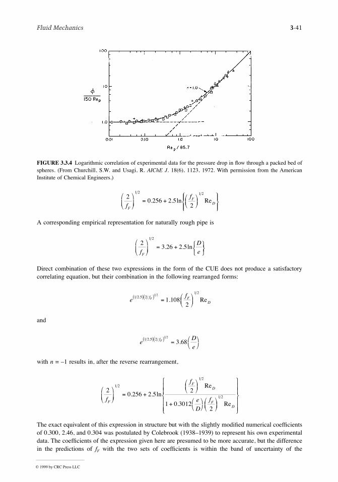
Fluid Mechanics 3-41
A corresponding empirical representation for naturally rough pipe is
Direct combination of these two expressions in the form of the CUE does not produce a satisfactorycorrelating equation, but their combination in the following rearranged forms:
and
with n = Ð1 results in, after the reverse rearrangement,
The exact equivalent of this expression in structure but with the slightly modiÞed numerical coefÞcientsof 0.300, 2.46, and 0.304 was postulated by Colebrook (1938Ð1939) to represent his own experimentaldata. The coefÞcients of the expression given here are presumed to be more accurate, but the differencein the predictions of fF with the two sets of coefÞcients is within the band of uncertainty of the
FIGURE 3.3.4 Logarithmic correlation of experimental data for the pressure drop in ßow through a packed bed ofspheres. (From Churchill, S.W. and Usagi, R. AIChE J. 18(6), 1123, 1972. With permission from the AmericanInstitute of Chemical Engineers.)
20 256 2 5
2
1 2 1 2
f
f
F
FD
æ
èç
ö
ø÷ = + æ
èç
öø÷
ìíï
îï
üýï
þï. . ln Re
23 26 2 5
1 2
f
D
eF
æ
èç
ö
ø÷ = + ì
íî
üýþ
. . ln
eff F
DF1 2 5 2
1 21 2
1 1082
. .( )( ) = æèç
öø÷ Re
eD
efF1 2 5 2
1 2
3 68. .( )( ) = æè
öø
20 256 2 5
2
1 0 30122
1 2
1 2
1 2f
f
e
D
fF
FD
FD
æ
èç
ö
ø÷ = +
æèç
öø÷
+ æè
öø
æèç
öø÷
ì
íïï
îïï
ü
ýïï
þïï
. . ln
.
Re
Re
© 1999 by CRC Press LLC
3-42 Section 3
experimental data. The turbulent regime of the Òfriction-factorÓ plot in most current textbooks andhandbooks is simply a graphical representation of the Colebrook equation. Experimental values are notincluded in such plots since e, the effective roughness of commercial pipes, is simply a correlating factorthat forces agreement with the Colebrook equation. Values of e for various types of pipe in variousservices are usually provided in an accompanying table, that thereby constitutes an integral part of thecorrelation.
The Laminar Region. The Fanning friction factor in the laminar regime of a round pipe (Red < 1800)is represented exactly by the following theoretical expression known as PoiseuilleÕs law: fF = 16/ReD.This equation may be rearranged as follows for convenience in combination with that for turbulent ßow:
The Transitional Regime. Experimental data as well as semitheoretical computed values for the limitingbehavior in the transition may be represented closely by (fF/2) = (ReD/37500)2. This expression may berewritten, in terms of (2/fF)1/2 and ReD(fF/2)1/2, as follows:
Overall Correlation. The following correlating equation for all ReD(fF/2)1/2 and e/D may now be con-structed by the combination of the expressions for the turbulent and transition regimes in the form ofthe CUE with n = 8, and then that expression and that for the laminar regime with n = Ð12, bothcomponents being chosen on the basis of experimental data and predicted values for the full regime oftransition:
The absolute value signs are only included for aesthetic reasons; the negative values of the logarithmicterm for very small values of ReD(fF/2)1/2 do not affect the numerical value of (2/fF)1/2 in the regime inwhich they occur. This overall expression appears to have a complicated structure, but it may readilybe recognized to reduce to its component parts when the corresponding term is large with respect to theother two. It is insensitive to the numerical values of the two arbitrary exponents. For example, doublingtheir values would have almost no effect on the predictions of (fF/2)1/2. The principal uncertainty isassociated with the expression for the transition regime, but the overall effect of the corresponding termis very small. The uncertainties associated with this correlating equation are common to most graphicalcorrelations and algebraic expressions for the friction factor, and are presumed to be fairly limited inmagnitude and to be associated primarily with the postulated value of e. Although the overall expressionis explicit in ReD(fF/2)1/2 rather than ReD, the latter quantity may readily be obtained simply by multiplyingthe postulated value of ReD(fF/2)1/2 by the computed values of (2/fF)1/2.
2 2
8
1 2 1 2
f
f
F
D Fæ
èç
ö
ø÷ =
( )Re
f
fF
D F2
37500
2
1 2
1 2
1 2
æèç
öø÷ =
( )æ
èçç
ö
ø÷÷Re
2 8
2
37500
22 5
1 108 2
1 0 3012 2
1 2
1 2
12
1 2
4 1 2
1 2
8
f f
f
f
e
af
F D F
D F
D F
D F
æ
èç
ö
ø÷ =
( )æ
èçç
ö
ø÷÷
é
ë
êêê
+( )
é
ë
êê
ù
û
úú
+( )
+ æè
öø ( )
ì
íïï
îïï
ü
ýïï
þïï
æ
è
çççç
ö
ø
Re
Re
Re
Re. ln
.
.
÷÷÷÷÷
ù
û
úúúúú
- -3 2 1 12
© 1999 by CRC Press LLC
Fluid Mechanics 3-43
References
Buckingham, E. 1914. On physically similar systems; illustrations of the use of dimensional equations.Phys. Rev., Ser. 2, 4(4):345Ð375.
Churchill, S.W. 1976. A comprehensive correlating equation for forced convection from plates. AIChEJ. 22(2):264Ð268.
Churchill, S.W. 1977. Comprehensive correlating equation for heat, mass and momentum transfer infully developed ßow in smooth tubes. Ind. Eng. Chem. Fundam. 16(1):109Ð116.
Churchill, S.W. 1979. The Interpretation and Use of Rate Data. The Rate Process Concept, rev. printing,Hemisphere Publishing Corp., Washington, D.C.
Churchill, S.W. 1981. The use of speculation and analysis in the development of correlations. Chem.Eng. Commun. 9:19Ð38.
Churchill, S.W. 1988a. Flow through porous media, Chapter 19 in Laminar Flows. The Practical Useof Theory, pp. 501Ð538, Butterworths, Boston.
Churchill, S.W. 1988b. Derivation, selection, evaluation and use of asymptotes. Chem. Eng. Technol.11:63Ð72.
Churchill, S.W. and Churchill, R.U. 1975. A general model for the effective viscosity of pseudoplasticand dilatant ßuids. Rheol. Acta. 14:404Ð409.
Churchill, S.W. and Usagi, R. 1972. A general expression for the correlation of rates of transfer andother phenomena. AIChE J. 18(6):1121Ð1128.
Churchill, S.W. and Usagi, R. 1974. A standardized procedure for the production of correlations in theform of a common empirical equation. Ind. Eng. Chem. Fundam. 13(1):39Ð44.
Colebrook, C.R. 1938Ð1939. Turbulent ßow in pipes with particular reference to the transition regionbetween the smooth and rough pipe laws. J. Inst. Civ. Eng. 11(5024):133Ð156.
Ergun, S. 1952. Fluid ßow through packed beds. Chem. Eng. Prog. 48(2):81Ð96.Hellums, J.D. and Churchill, S.W. 1964. SimpliÞcations of the mathematical description of boundary
and initial value problems. AIChE J. 10(1):110Ð114.Wilkie, D. 1985. The correlation of engineering data reconsidered. Int. J. Heat Fluid Flow. 8(2):99Ð103.Zlokarnik, M. 1991. Dimensional Analysis and Scale-Up in Chemical Engineering. Springer-Verlag,
Berlin.
© 1999 by CRC Press LLC
3-44 Section 3
3.4 Hydraulics of Pipe Systems
J. Paul Tullis
Basic Computations
Equations
Solving ßuid ßow problems involves the application of one or more of the three basic equations:continuity, momentum, and energy. These three basic tools are developed from the law of conservationof mass, NewtonÕs second law of motion, and the Þrst law of thermodynamics.
The simplest form of the continuity equation is for one-dimensional incompressible steady ßow in aconduit. Applying continuity between any two sections gives
(3.4.1)
For a variable density the equation can be written
(3.4.2)
in which A is the cross-sectional area of the pipe, V is the mean velocity at that same location, Q is theßow rate, r is the ßuid density, and is the mass ßow rate. The equations are valid for any rigidconduit as long as there is no addition or loss of liquid between the sections.
For steady state pipe ßow, the momentum equation relates the net force in a given direction (Fx) actingon a control volume (a section of the ßuid inside the pipe), to the net momentum ßux through the controlvolume.
(3.4.3)
For incompressible ßow this equation can be reduced to
(3.4.4.)
These equations can easily be applied to a three-dimensional ßow problem by adding equations in they and z directions.
A general form of the energy equation (see Chapter 2) applicable to incompressible pipe or duct ßow
(3.4.5)
The units are energy per unit weight of liquid: ft á lb/lb or N á m/N which reduce to ft or m. The Þrstthree terms are pressure head (P/g), elevation head (Z) (above some datum), and velocity head (V2/2g).The last three terms on the right side of the equation are the total dynamic head added by a pump (Hp)or removed by a turbine (Ht) and the friction plus minor head losses (Hf). The sum of the Þrst threeterms in Equation 3.4.5 is deÞned as the total head, and the sum of the pressure and elevation heads isreferred to as the piezometric head.
The purpose of this section is to determine the pressure changes resulting from incompressible ßowin pipe systems. Since pipes of circular cross sections are most common in engineering application, theanalysis in this section will be performed for circular geometry. However, the results can be generalizedfor a pipe of noncircular geometry by substituting for the diameter D in any of the equations, the hydraulicdiameter, Dh, deÞned as
A V A V Q1 1 2 2= =
r r1 1 1 2 2 2A V A V m= = Ç
Çm
F A V V A V Vx x x= -r r2 2 2 2 1 1 1 1
F Q V Vx x x= -( )r 2 1
PZ
V
g
PZ
V
gH H Hp t f
11
12
22
22
2 2g g+ + = + + - + +
© 1999 by CRC Press LLC
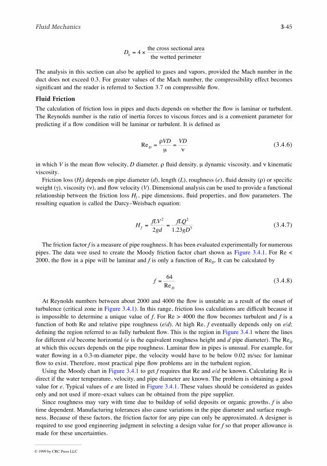
Fluid Mechanics 3-45
The analysis in this section can also be applied to gases and vapors, provided the Mach number in theduct does not exceed 0.3. For greater values of the Mach number, the compressibility effect becomessigniÞcant and the reader is referred to Section 3.7 on compressible ßow.
Fluid Friction
The calculation of friction loss in pipes and ducts depends on whether the ßow is laminar or turbulent.The Reynolds number is the ratio of inertia forces to viscous forces and is a convenient parameter forpredicting if a ßow condition will be laminar or turbulent. It is deÞned as
(3.4.6)
in which V is the mean ßow velocity, D diameter, r ßuid density, m dynamic viscosity, and n kinematicviscosity.
Friction loss (Hf) depends on pipe diameter (d), length (L), roughness (e), ßuid density (r) or speciÞcweight (g), viscosity (n), and ßow velocity (V). Dimensional analysis can be used to provide a functionalrelationship between the friction loss Hf , pipe dimensions, ßuid properties, and ßow parameters. Theresulting equation is called the DarcyÐWeisbach equation:
(3.4.7)
The friction factor f is a measure of pipe roughness. It has been evaluated experimentally for numerouspipes. The data wee used to create the Moody friction factor chart shown as Figure 3.4.1. For Re <2000, the ßow in a pipe will be laminar and f is only a function of ReD. It can be calculated by
(3.4.8)
At Reynolds numbers between about 2000 and 4000 the ßow is unstable as a result of the onset ofturbulence (critical zone in Figure 3.4.1). In this range, friction loss calculations are difÞcult because itis impossible to determine a unique value of f. For Re > 4000 the ßow becomes turbulent and f is afunction of both Re and relative pipe roughness (e/d). At high Re, f eventually depends only on e/d;deÞning the region referred to as fully turbulent ßow. This is the region in Figure 3.4.1 where the linesfor different e/d become horizontal (e is the equivalent roughness height and d pipe diameter). The ReD
at which this occurs depends on the pipe roughness. Laminar ßow in pipes is unusual. For example, forwater ßowing in a 0.3-m-diameter pipe, the velocity would have to be below 0.02 m/sec for laminarßow to exist. Therefore, most practical pipe ßow problems are in the turbulent region.
Using the Moody chart in Figure 3.4.1 to get f requires that Re and e/d be known. Calculating Re isdirect if the water temperature, velocity, and pipe diameter are known. The problem is obtaining a goodvalue for e. Typical values of e are listed in Figure 3.4.1. These values should be considered as guidesonly and not used if moreÐexact values can be obtained from the pipe supplier.
Since roughness may vary with time due to buildup of solid deposits or organic growths, f is alsotime dependent. Manufacturing tolerances also cause variations in the pipe diameter and surface rough-ness. Because of these factors, the friction factor for any pipe can only be approximated. A designer isrequired to use good engineering judgment in selecting a design value for f so that proper allowance ismade for these uncertainties.
Dh = ´4the cross sectional area
the wetted perimeter
ReD
VD VD= =
rm n
HfLV
gd
fLQ
gDf = =2 2
52 1 23.
fD
=64
Re
© 1999 by CRC Press LLC
3-46 Section 3
For noncircular pipes, the only change in the friction loss equation is the use of an equivalent diameterÑ based on the hydraulic radius (R), i.e., d = 4R Ñ in place of the circular pipe diameter d. R is theratio of the ßow area to the wetter perimeter.
Wood (1966) developed equations which can be used in place of the Moody diagram to estimate ffor Re > 104 and 10Ð5 < k < 0.04 (k = e/d).
(3.4.9)
The practical problem is still obtaining a reliable value for e. It cannot be directly measured but mustbe determined from friction loss tests of the pipe.
An exact solution using the DarcyÐWeisbach equation can require a trial-and-error solution becauseof the dependency of f on Re if either the ßow or pipe diameter are not known. A typical approach tosolving this problem is to estimate a reasonable ßuid velocity to calculate Re and obtain f from theMoody chart or Equation (3.4.9). Next, calculate a new velocity and repeat until the solution converges.Converging on a solution is greatly simpliÞed with programmable calculators and a variety of softwareavailable for computer.
For long gravity ßow pipelines, the starting point in selecting the pipe diameter is to determine thesmallest pipe that can pass the required ßow without friction loss exceeding the available head. Forpumped systems, the selection must be based on an economic analysis that compares the pipe cost withthe cost of building and operating the pumping plant.
Local Losses
Flow through valves, oriÞces, elbows, transitions, etc. causes ßow separation which results in thegeneration and dissipation of turbulent eddies. For short systems containing many bends, valves, tees,
FIGURE 3.4.1 The Moody diagram.
f a b c= + -Re
a k k b k c k= + = =0 094 0 53 88 1 620 225 0 44 0 134. . , , .. . .
© 1999 by CRC Press LLC
Fluid Mechanics 3-47
etc. local or minor losses can exceed friction losses. The head loss hl associated with the dissipationcaused by a minor loss is proportional to the velocity head and can be accounted for as a minor or localloss using the following equation.
(3.4.10)
in which Kl is the minor loss coefÞcient and Am is the area of the pipe at the inlet to the local loss. Theloss coefÞcient Kl is analogous to fL/d in Equation 3.4.7.
The summation of all friction and local losses in a pipe system can be expressed as
(3.4.11)
(3.4.12)
in which
(3.4.13)
It is important to use the correct pipe diameter for each pipe section and local loss.In the past some have expressed the local losses as an equivalent pipe length: L/d = Kl/f. It simply
represents the length of pipe that produces the same head loss as the local or minor loss. This is asimple, but not a completely accurate method of including local losses. The problem with this approachis that since the friction coefÞcient varies from pipe to pipe, the equivalent length will not have a uniquevalue. When local losses are truly minor, this problem becomes academic because the error onlyinßuences losses which make up a small percentage of the total. For cases where accurate evaluationof all losses is important, it is recommended that the minor loss coefÞcients Kl be used rather than anequivalent length.
The challenging part of making minor loss calculations is obtaining reliable values of Kl. The Þnalresults cannot be any more accurate than the input data. If the pipe is long, the friction losses may belarge compared with the minor losses and approximate values of Kl will be sufÞcient. However, for shortsystems with many pipe Þttings, the local losses can represent a signiÞcant portion of the total systemlosses, and they should be accurately determined. Numerous factors inßuence Kl. For example, forelbows, Kl is inßuenced by the shape of the conduit (rectangular vs. circular), by the radius of the bend,the bend angle, the Reynolds number, and the length of the outlet pipe. For dividing or combining teesor Y-branches, the percent division of ßow and the change in pipe diameter must also be included whenestimating Kl. One factor which is important for systems where local losses are signiÞcant is theinteraction between components placed close together. Depending on the type, orientation, and spacingof the components, the total loss coefÞcient may be greater or less than the simple sum of the individualKl values.
Comparing the magnitude of S(fL/2gA2) to S will determine how much care should begiven to the selection of the Kl values. Typical values of Kl are listed in Table 3.4.1 (Tullis, 1989). Whenmore comprehensive information on loss coefÞcients is needed, the reader is referred to Miller (1990).
h KQ
gAl lm
=( )
2
22
H h hf f l= +
HfL
gdA
K
gAQ CQf
p
l
m
=æ
èç
ö
ø÷ +
æ
èç
ö
ø÷
é
ëêê
ù
ûúú
=å å2 22 22 2
CfL
gdA
K
gAp
l
m
=æ
èç
ö
ø÷ +
æ
èç
ö
ø÷å å2 22 2
( / )K gAl m2 2
© 1999 by CRC Press LLC
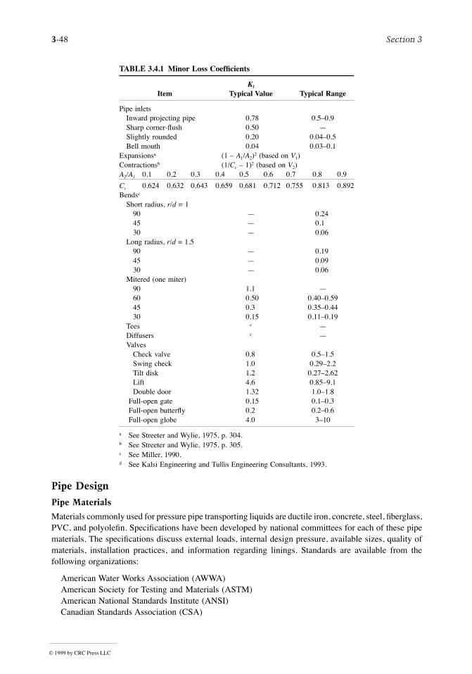
3-48 Section 3
Pipe Design
Pipe Materials
Materials commonly used for pressure pipe transporting liquids are ductile iron, concrete, steel, Þberglass,PVC, and polyoleÞn. SpeciÞcations have been developed by national committees for each of these pipematerials. The speciÞcations discuss external loads, internal design pressure, available sizes, quality ofmaterials, installation practices, and information regarding linings. Standards are available from thefollowing organizations:
American Water Works Association (AWWA)American Society for Testing and Materials (ASTM)American National Standards Institute (ANSI)Canadian Standards Association (CSA)
TABLE 3.4.1 Minor Loss CoefÞcients
Kl
Item Typical Value Typical Range
Pipe inletsInward projecting pipe 0.78 0.5Ð0.9Sharp corner-ßush 0.50 ÑSlightly rounded 0.20 0.04Ð0.5Bell mouth 0.04 0.03Ð0.1
Expansionsa (1 Ð A1/A2)2 (based on V1)Contractionsb (1/Cc Ð 1)2 (based on V2)A2/A1 0.1 0.2 0.3 0.4 0.5 0.6 0.7 0.8 0.9
Cc 0.624 0.632 0.643 0.659 0.681 0.712 0.755 0.813 0.892Bendsc
Short radius, r/d = 190 Ñ 0.2445 Ñ 0.130 Ñ 0.06
Long radius, r/d = 1.590 Ñ 0.1945 Ñ 0.0930 Ñ 0.06
Mitered (one miter)90 1.1 Ñ60 0.50 0.40Ð0.5945 0.3 0.35Ð0.4430 0.15 0.11Ð0.19
Tees c ÑDiffusers c ÑValves
Check valve 0.8 0.5Ð1.5Swing check 1.0 0.29Ð2.2Tilt disk 1.2 0.27Ð2.62Lift 4.6 0.85Ð9.1Double door 1.32 1.0Ð1.8
Full-open gate 0.15 0.1Ð0.3 Full-open butterßy 0.2 0.2Ð0.6 Full-open globe 4.0 3Ð10
a See Streeter and Wylie, 1975, p. 304.b See Streeter and Wylie, 1975, p. 305.c See Miller, 1990.d See Kalsi Engineering and Tullis Engineering Consultants, 1993.
© 1999 by CRC Press LLC
Fluid Mechanics 3-49
Federal SpeciÞcations (FED)Plastic Pipe Institute (PPI)
In addition, manuals and other standards have been published by various manufacturers and manu-facturerÕs associations. All of these speciÞcations and standards should be used to guide the selectionof pipe material. ASCE (1992) contains a description of each of these pipe materials and a list of thespeciÞcations for the various organizations which apply to each material. It also discusses the variouspipe-lining materials available for corrosion protection.
For air- and low-pressure liquid applications one can use unreinforced concrete, corrugated steel,smooth sheet metal, spiral rib (sheet metal), and HDPE (high-density polyethylene) pipe. The choice ofa material for a given application depends on pipe size, pressure requirements, resistance to collapsefrom internal vacuums, external loads, resistance to internal and external corrosion, ease of handlingand installing, useful life, and economics.
Pressure Class Guidelines
Procedures for selecting the pressure class of pipe vary with the type of pipe material. Guidelines fordifferent types of materials are available from AWWA, ASTM, ANSI, CSA, FED, PPI and from thepipe manufacturers. These speciÞcations should be obtained and studied for the pipe materials beingconsidered.
The primary factors governing the selection of a pipe pressure class are (1) the maximum steady stateoperating pressure, (2) surge and transient pressures, (3) external earth loads and live loads, (4) variationof pipe properties with temperature or long-time loading effects, and (5) damage that could result fromhandling, shipping, and installing or reduction in strength due to chemical attack or other aging factors.The inßuence of the Þrst three items can be quantiÞed, but the last two are very subjective and aregenerally accounted for with a safety factor which is the ratio of the burst pressure to the rated pressure.
There is no standard procedure on how large the safety factor should be or on how the safety factorshould be applied. Some may feel that it is large enough to account for all of the uncertainties. Pastfailures of pipelines designed using this assumption prove that it is not always a reliable approach. Theprocedure recommended by the author is to select a pipe pressure class based on the internal designpressure (IDP) deÞned as
(3.4.14)
in which Pmax is the maximum steady state operating pressure, Ps is the surge or water hammer pressure,and SF is the safety factor applied to take care of the unknowns (items 3 to 5) just enumerated. A safetyfactor between 3 and 4 is typical.
The maximum steady state operating pressure (Pmax) in a gravity ßow system is usually the differencebetween the maximum reservoir elevation and the lowest elevation of the pipe. For a pumped system itis usually the pump shutoff head calculated based on the lowest elevation of the pipe.
Surge and transient pressures depend on the speciÞc pipe system design and operation. Accuratelydetermining Ps requires analyzing the system using modern computer techniques. The most commonlyused method is the ÒMethod of CharacteristicsÓ (Tullis, 1989; Wylie and Streeter, 1993). Some of thedesign standards give general guidelines to predict Ps that can be used if a detailed transient analysis isnot made. However, transients are complex enough that simple Òrules of thumbÓ are seldom accurateenough. Transients are discussed again in a later subsection.
Selection of wall thickness for larger pipes is often more dependent on collapse pressure and handlingloads than it is on burst pressure. A thin-wall, large-diameter pipe may be adequate for resisting relativelyhigh internal pressures but may collapse under negative internal pressure or, if the pipe is buried, thesoil and groundwater pressure plus live loads may be sufÞcient to cause collapse even if the pressureinside the pipe is positive.
IDP = SFP Psmax +( )
© 1999 by CRC Press LLC
3-50 Section 3
External Loads
There are situations where the external load is the controlling factor determining if the pipe will collapse.The magnitude of the external load depends on the diameter of the pipe, the pipe material, the ovality(out of roundness) of the pipe cross section, the trench width, the depth of cover, the speciÞc weight ofthe soil, the degree of soil saturation, the type of backÞll material, the method used to backÞll, the degreeof compaction, and live loads. The earth load increases with width and depth of the trench, and the liveload reduces with depth of cover. The cumulative effect of all these sources of external loading requiresconsiderable study and analysis.
There are no simple guidelines for evaluating external pipe loads. Because of the complexity of thisanalysis, the default is to assume that the safety factor is adequate to account for external loads as wellas the other factors already mentioned. One should not allow the safety factor to replace engineeringjudgment and calculations. One option to partially compensate for the lack of a detailed analysis is touse a higher-pressure class of pipe in areas where there will be large live loads or where the earth loadingis unusually high. One should consider the cost of a pipe failure caused by external loads comparedwith the cost of using a thicker pipe or the cost of performing a detailed analysis. Those interested inthe details of performing calculations of earth loading should be Spranger and Handy, 1973.
Limiting Velocities
There are concerns about upper and lower velocity limits. If the velocity is too low, problems maydevelop due to settling of suspended solids and air being trapped at high points and along the crown ofthe pipe. The safe lower velocity limit to avoid collecting air and sediment depends on the amount andtype of sediment and on the pipe diameter and pipe proÞle. Velocities greater than about 1 m/sec (3ft/sec) are usually sufÞcient to move trapped air to air release valves and keep the sediment in suspension.
Problems associated with high velocities are (1) erosion of the pipe wall or liner (especially if coarsesuspended sediment is present), (2) cavitation at control valves and other restrictions, (3) increasedpumping costs, (4) removal of air at air release valves, (5) increased operator size and concern aboutvalve shaft failures due to excessive ßow torques, and (6) an increased risk of hydraulic transients. Eachof these should be considered before making the Þnal pipe diameter selection. A typical upper velocityfor many applications if 6 m/sec (20 ft/sec). However, with proper pipe design and analysis (of thepreceding six conditions), plus proper valve selection, much higher velocities can be tolerated. A typicalupper velocity limit for standard pipes and valves is about 6 m/sec (20 ft/sec). However, with properdesign and analysis, much higher velocities can be tolerated.
Valve Selection
Valves serve a variety of functions. Some function as isolation or block valves that are either full openor closed. Control valves are used to regulate ßow or pressure and must operate over a wide range ofvalve openings. Check valves prevent reverse ßow, and air valves release air during initial Þlling andair that is collected during operation and admit air when the pipe is drained.
Control Valves
For many ßow control applications it is desirable to select a valve that has linear control characteristics.This means that if you close the valve 10%, the ßow reduces about 10%. Unfortunately, this is seldompossible since the ability of a valve to control ßow depends as much on the system as it does on thedesign of the valve. The same valve that operates linearly in one system may not in another.
Selecting the proper ßow control valve should consider the following criteria:
1. The valve should not produce excessive pressure drop when full open.2. The valve should control over at least 50% of its movement.3. At maximum ßow, the operating torque must not exceed the capacity of the operator or valve
shaft and connections.4. The valve should not be subjected to excessive cavitation.
© 1999 by CRC Press LLC
Fluid Mechanics 3-51
5. Pressure transients should not exceed the safe limits of the system.6. Some valves should not be operated at very small openings. Other valves should be operated near
full open.
Controllability. To demonstrate the relationship between a valve and system, consider a butterßy valvethat will be used to control the ßow between two reservoirs with an elevation difference of DZ. SystemA is a short pipe (0.3 m dia., 100 m long, DZ = 10 m) where pipe friction is small = 46.9,and System B is a long pipe (0.3 m dia., 10,000 m long, DZ = 200 m) with high friction =4690. Initially, assume that the same butterßy valve will be used in both pipes and it will be the samesize as the pipe. The ßow can be calculated using the energy equation (Equation 3.4.5) and the systemloss equation (Equation (3.4.12):
(3.4.15)
For the valve, assume that the Kl full open is 0.2 and at 50% open it is 9.0. Correspondingly, = 1.905 and 85.7. For System A, the ßow with the valve full open will be 0.453 m3/sec and at 50% open0.275 m3/sec, a reduction of 39%. Repeating these calculations over the full range of valve openingswould show that the ßow for System A reduces almost linearly as the valve closes.
For System B, the ßow with the valve full open will be 0.206 m3/sec and at 50% open 0.205 m3/sec,a reduction of less than 1%. For System B the valve does not control until the valve loss, expressed by
becomes a signiÞcant part of the friction term (4690). The same valve in System B will notstart to control the ßow until it has closed more than 50%. A line-size butterßy valve is obviously nota good choice for a control valve in System B. One solution to this problem is to use a smaller valve.If the butterßy valve installed in System B was half the pipe diameter, it would control the ßow overmore of the stroke of the valve.
The range of opening over which the valve controls the ßow also has a signiÞcant effect on the safeclosure time for control valves. Transient pressures are created when there is a sudden change in theßow. Most valve operators close the valve at a constant speed. If the valve does not control until it ismore than 50% closed, over half of the closing time is wasted and the effective valve closure time isless than half the total closing time. This will increase the magnitude of the transients that will begenerated.
Torque. To be sure that the valve shaft, connections, and operator are properly sized, the maximumtorque or thrust must be known. If the maximum force exceeds operator capacity, it will not be able toopen and close the valve under extreme ßow conditions. If the shaft and connectors are underdesigned,the valve may fail and slam shut causing a severe transient.
For quarter-turn valves, the force required to operate a valve consists of seating, bearing, and packingfriction, hydrodynamic (ßow) forces, and inertial forces. These forces are best determined experimentally.A key step in applying experimental torque information is the determination of the ßow condition creatingmaximum torque. This requires that the system be analyzed for all possible operating conditions andvalve openings. For a given size and type of valve, the ßow torque depends on the torque coefÞcient(which is dependent on the speciÞc valve design) and the pressure drop which, in turn, depends on theßow. In short systems where there is little friction loss and high velocities, a quarter-turn valve will seemaximum torques at large openings where the ßow is high. In long systems with high reservoir headsand smaller velocities, the same valve will see maximum torque at small openings where the pressuredrop is high.
One situation where it is easy to overlook the condition causing maximum torque is with parallelpumps. Each pump normally will have a discharge control valve. The maximum system ßow occurswith all three pumps operating. However, the ßow and the torque for any of the pump discharge valves
fL gdAp/2 2
fL gdAp/2 2
QZ
fL
gdA
K
gAp
l
m
=D
2 22 2
æ
èç
ö
ø÷ +
æ
èç
ö
ø÷
é
ëêê
ù
ûúúå å
K gAl m/2 2
K gAl m/2 2
© 1999 by CRC Press LLC
3-52 Section 3
is maximum for only one pump operating. One speciÞc example (Tullis, 1989) showed that the torqueon a butterßy valve was three times higher when one pump was operating compared with three pumpsoperating in parallel.
Cavitation. Cavitation is frequently an important consideration in selection and operation of controlvalves. It is necessary to determine if cavitation will exist, evaluate its intensity, and estimate its effecton the system and environment. Cavitation can cause noise, vibration, and erosion damage and candecrease performance. The analysis should consider the full range of operation. Some valves cavitateworst at small openings and others cavitate heavily near full open. It depends on both the system andthe valve design. If cavitation is ignored in the design and selection of the valves, repairs and replacementof the valves may be necessary. Information for making a complete cavitation analysis is beyond thescope of this section. Detailed information on the process to design for cavitation is contained in Tullis(1989; 1993).
The Þrst step in a cavitation analysis is selecting the acceptable level of cavitation. Experimental dataare available for four limits: incipient (light, intermittent noise), critical (light, steady noise), incipientdamage (pitting damage begins), and choking (very heavy damage and performance drops off). Limitedcavitation data are available for each of these limits (Tullis, 1989; 1993). Choosing a cavitation limitdepends on several factors related to the operating requirements, expected life, location of the device,details of the design, and economics. For long-term operation of a control valve in a system where noisecan be tolerated, the valve should never operate beyond incipient damage. In systems where noise isobjectionable, critical cavitation would be a better operating limit.
Using a choking cavitation as a design limit is often misused. It is generally appropriate as a designlimit for valves that only operate for short periods of time, such as a pressure relief valve. The intensityof cavitation and the corresponding noise vibration and erosion damage at the valve are at their maximumjust before a valve chokes. If the valve operates beyond choking (sometimes referred to as supercavita-tion), the collapse of the vapor cavities occurs remote from the valve. Little damage is likely to occurat the valve, but farther downstream serious vibration and material erosion problems can occur.
If the cavitation analysis indicates that the valve, oriÞce, or other device will be operating at a cavitationlevel greater than can be tolerated, various techniques can be used to limit the level of cavitation. Oneis to select a different type of valve. Recent developments in valve design have produced a new generationof valves that are more resistant to cavitation. Most of them operate on the principle of dropping thepressure in stages. They usually have multiple paths with numerous sharp turns or oriÞces in series. Twolimitations to these valves are that they often have high pressure drops (even when full open), and theyare only usable with clean ßuids.
A similar approach is to place multiple conventional valves in series or a valve in series with oriÞceplates. Proper spacing of valves and oriÞces placed in series is important. The spacing between valvesdepends upon the type. For butterßy valves it is necessary to have between Þve and eight diameters ofpipe between valves to prevent ßutter of the leaf of the downstream valve and to obtain the normalpressure drop at each valve. For globe, cone, and other types of valves, it is possible to bolt them ßangeto ßange and have satisfactory operation.
For some applications another way to suppress cavitation is to use a free-discharge valve that is ventedso cavitation cannot occur. There are valves speciÞcally designed for this application. Some conventionalvalves can also be used for free discharge, if they can be adequately vented.
Cavitation damage can be suppressed by plating critical areas of the pipe and valve with cavitation-resistant materials. Based on tests using a magnetostriction device, data show that there is a wide variationin the resistance of the various types of material. Limited testing has been done on the erosion resistanceof different materials and coating to cavitation in ßowing systems. The available data show that thereis less variation in the damage resistance of materials in actual ßowing systems. However, experiencehas shown the plating parts of the valve with the right material will extend valve life.
Injecting air to suppress cavitation is a technique which has been used for many years with varyingdegrees of success. The most common mistake is placing the air injection port in the wrong location so
© 1999 by CRC Press LLC
Fluid Mechanics 3-53
the air does not get to the cavitation zone. If an adequate amount of air is injected into the proper region,the noise, vibrations, and erosion damage can be signiÞcantly reduced. The air provides a cushioningeffect reducing the noise, vibration, and erosion damage. If the system can tolerate some air beinginjected, aeration is usually the cheapest and best remedy for cavitation.
Transients. Transient pressures can occur during Þlling and ßushing air from the line, while operatingvalves, and when starting or stopping pumps. If adequate design provisions and operational proceduresare not established, the transient pressure can easily exceed the safe operating pressure of the pipe. Asystem should be analyzed to determine the type and magnitudes of possible hydraulic transients. Thebasic cause is rapid changes in velocity. The larger the incremental velocity change and the faster thatchange takes place, the greater will be the transient pressure. If the piping system is not designed towithstand the high transient pressures, or if controls are not included to limit the pressure, rupture ofthe pipe or damage to equipment can result.
All pipelines experience transients. Whether or not the transient creates operational problems or pipefailure depends upon its magnitude and the ability of the pipes and mechanical equipment to toleratehigh pressures without damage. For example, an unreinforced concrete pipeline may have a transientpressure head allowance of only a meter above its operating pressure before damage can occur. For suchsituations even slow closing of control valves or minor interruptions of ßow due to any cause may createsufÞcient transient pressures to rupture the pipeline. In contrast, steel and plastic pipes can take relativelyhigh transient pressures without failure.
Transients caused by slow velocity changes, such as the rise and fall of the water level in a surgetank, are called surges. Surge analysis, or Òrigid column theoryÓ involves mathematical or numericalsolution of simple ordinary differential equations. The compressibility of the ßuid and the elasticity ofthe conduit are ignored, and the entire column of ßuid is assumed to move as a rigid body.
When changes in velocity occur rapidly, both the compressibility of the liquid and the elasticity ofthe pipe must be included in the analysis. This procedure is often called ÒelasticÓ or ÒwaterhammerÓanalysis and involves tracking acoustic pressure waves through the pipe. The solution requires solvingpartial differential equations.
An equation predicting the head rise DH caused by a sudden change of velocity DV = V2 Ð V1 can bederived by applying the unsteady momentum equation to a control volume of a section of the pipe wherethe change of ßow is occurring. Consider a partial valve closure which instantly reduces the velocityby an amount DV. Reduction of the velocity can only be accomplished by an increase in the pressureupstream from the valve. This creates a pressure wave of magnitude DH which travels up the pipe atthe acoustic velocity a. The increased pressure compresses the liquid and expands the pipe. The transienthead rise due to an incremental change in velocity is
(3.4.16)
This equation is easy to use for multiple incremental changes of velocity as long as the Þrst wave hasnot been reßected back to the point of origin.
The derivation of Equation (3.4.16) is based on an assumption of an instant velocity change. For avalve closing at the end of the pipe, instant closure actually refers to a Þnite time. It is the longest timethat a valve can be closed and still cause a pressure rise equal to that of an instant closure. Normally,it is equal to 2L/a sec (which is the time required for the Þrst pressure wave to travel to and from theother end of the pipe of length L); the head rise at the valve will be the same as if the valve were closedinstantly. The 2L/a time is therefore often the instant closure time.
For a valve at the end of a long pipeline, the instant closure time can be considerably greater than2L/a. This is because when the friction loss coefÞcient fL/d is much greater than the loss coefÞcient forthe valve Kl, the valve can be closed a long way before the ßow changes. This dead time must be addedto the 2L/a time to identify the actual instant closure time. To avoid the maximum potential transientpressure rise, the valve must be closed much slower than the instant closure time.
D D DH V g V= -a a, for @
© 1999 by CRC Press LLC
3-54 Section 3
Computational techniques for estimating transient pressures caused by unsteady ßow in pipelines aretoo complex to be done with simple hand calculations. The solution involves solving partial differentialequations based on the equations of motion and continuity. These equations are normally solved by themethod of characteristics. This technique transforms the equations into total differential equations. Afterintegration, the equations can be solved numerically by Þnite differences. This analysis provides equa-tions that can be used to predict the ßow and head at any interior pipe section at any time (Tullis, 1989;Wiley and Streeter, 1993).
To complete the analysis, equations describing the boundary conditions are required. Typical boundaryconditions are the connection of a pipe to a reservoir, a valve, changes in pipe diameter or material, pipejunctions, etc. Friction loss is included in the development of the basic equations and minor losses arehandled as boundary conditions. The analysis properly models friction and the propagation and reßectionsof the pressure wave. It can also be used for surge calculations.
It is recommended that every pipe system should have at least a cursory transient analysis performedto identify the possibility of serious transients and decide whether or not a detailed analysis is necessary.If an analysis indicates that transients are a problem, the types of solutions available to the engineerinclude
1. Increasing the closing time of control valves.2. Using a smaller valve to provide better control.3. Designing special facilities for Þlling, ßushing, and removing air from pipelines.4. Increasing the pressure class of the pipeline.5. Limiting the ßow velocity.6. Using pressure relief valves, surge tanks, air chambers, etc.
Check Valves
Selecting the wrong type or size of check valve can result in poor performance, severe transients, andfrequent repairs (Kalsi, 1993). Proper check valve selection requires understanding the characteristicsof the various types of check valves and analyzing how they will function as a part of the system inwhich they will be installed. A check valve that operates satisfactorily in one system may be totallyinadequate in another. Each valve type has unique characteristics that give it advantages or disadvantagescompared with the others. The characteristics of check valves that describe their hydraulic performanceand which should be considered in the selection process include
1. Opening characteristics, i.e., velocity vs. disk position data.2. Velocity required to fully open and Þrmly backseat the disk.3. Pressure drop at maximum ßow.4. Stability of the disk at partial openings.5. Sensitivity of disk ßutter to upstream disturbances.6. Speed of valve closure compared with the rate of ßow reversal of the system.
Disk stability varies with ßow rate, disk position, and upstream disturbances and is an important factorin determining the useful life of a check valve. For most applications it is preferable to size the checkvalve so that the disk is fully open and Þrmly backseated at normal ßow rates. One of the worst designerrors is to oversize a check valve that is located just downstream from a disturbance such as a pump,elbow, or control valve. If the disk does not fully open, it will be subjected to severe motion that willaccelerate wear. To avoid this problem, it may be necessary to select a check valve that is smaller thanthe pipe size.
The transient pressure rise generated at check valve closure is another important consideration. Thepressure rise is a function of how fast the valve disk closes compared with how fast the ßow in thesystem reverses. The speed that the ßow in a system reverses depends on the system. In systems whererapid ßow reversals occur, the disk can slam shut causing a pressure transient (Thorley, 1989).
© 1999 by CRC Press LLC
Fluid Mechanics 3-55
The closing speed of a valve is determined by the mass of the disk, the forces closing the disk, andthe distance of travel from full open to closed. Fast closing valves have the following properties: thedisk (including all moving parts) is lightweight, closure is assisted by springs, and the full stroke of thedisk is short. Swing check valves are the slowest-closing valves because they violate all three of thesecriteria; i.e., they have heavy disks, no springs, and long disk travel. The nozzle check valve is one ofthe fastest-closing valves because the closing element is light, is spring loaded, and has a short stroke.The silent, duo, double door, and lift check valves with springs are similar to nozzle valves in theirclosing times, mainly because of the closing force of the spring.
Systems where rapid ßow reversals occur include parallel pumps, where one pump is stopped whilethe others are still operating, and systems that have air chambers or surge tanks close to the check valve.For these systems there is a high-energy source downstream from the check valve to cause the ßow toquickly reverse. As the disk nears its seat, it starts to restrict the reverse ßow. This builds up the pressure,accelerates the disk, and slams it into the seat. Results of laboratory experiments, Þeld tests, and computersimulations show that dramatic reductions in the transient pressures at disk closure can be achieved byreplacing a slow-closing swing check valve with a fast-acting check valve. For example, in a systemcontaining parallel pumps where the transient was generated by stopping one of the pumps, the peaktransient pressure was reduced from 745 to 76 kPa when a swing check was replaced with a nozzlecheck valve. Such a change improved performance and signiÞcantly reduced maintenance.
Air Valves
There are three types of automatic air valves: (1) air/vacuum valves, (2) air release valves, and (3)combination valves. The air/vacuum valve is designed for releasing air while the pipe is being Þlled andfor admitting air when the pipe is being drained. The valve must be large enough that it can admit andexpel large quantities of air at a low pressure differential. The outlet oriÞce is generally the same diameteras the inlet pipe.
These valves typically contain a ßoat, which rises and closes the oriÞce as the valve body Þlls withwater. Once the line is pressurized, this type of valve cannot reopen to remove air that may subsequentlyaccumulate until the pressure becomes negative, allowing the ßoat to drop. If the pressure becomesnegative during a transient or while draining, the ßoat drops and admits air into the line. For thin-walledpipes that can collapse under internal vacuums, the air/vacuum valves should be sized for a full pipebreak at the lowest pipe elevation. The vacuum valve must supply an air ßow equal to the maximumdrainage rate of the water from the pipe break and at an internal pipe pressure above the pipe collapsepressure.
The critical factor in sizing air/vacuum valves is usually the air ßow rate to protect the pipe from afull pipe break. Since a pipe is Þlled much slower than it would drain during a full break, the selectedvalve will be sized so that the air is expelled during Þlling without pressurizing the pipe. Sizing chartsare provided by manufacturers.
Air release valves contain a small oriÞce and are designed to release small quantities of pressurizedair that are trapped during Þlling and that accumulate after initial Þlling and pressurization. The smalloriÞce is controlled by a plunger activated by a ßoat at the end of a lever arm. As air accumulates inthe valve body, the ßoat drops and opens the oriÞce. As the air is expelled, the ßoat rises and closes offthe oriÞce. Sizing air release valves requires an estimate of the amount of pressurized air that must beexpelled. This is determined by the Þlling procedure and any source of air that can be admitted into thepipe or be degassed from the liquid during operation.
The combination valve is actually two valves: a large valve that functions as an air/vacuum valve anda small one that functions as an air release valve. The installation can either consist of an air/vacuumvalve and an air release valve plumbed in parallel, or the two can be housed in a single valve body.Most air valve installations require combination valves.
One caution is that manual air release valves should be avoided because improper operation of themcan be very dangerous. If the system is pressurized with the manual air valves closed, the trapped air
© 1999 by CRC Press LLC
3-56 Section 3
will be pressurized to full system pressure. When the air valve is manually opened, the pressurized aircan cause rapid acceleration of the liquid and generate serious transients when the water is deceleratedas it hits the air valve. If manual air valves are installed, they should be very small so the air releaserate is controlled to a safe rate.
Locating air valves in a piping system depends on the pipe proÞle, pipe length, and ßow rates.Preferably, pipes should be laid to grade with valves placed at the high points or at intervals if there areno high points. One should use engineering judgment when deÞning a high point. If the pipe has numeroushigh points that are close together, or if the high points are not pronounced, it will not be necessary tohave an air valve at each high point. If the liquid ßow velocity is above about 1 m/sec (3 ft/sec), theßowing water can move the entrained air past intermediate high points to a downstream air valve.Releasing the air through an air valve prevents any sizable air pockets under high pressure from formingin the pipe. Trapped air under high pressure is extremely dangerous.
Velocity of the ßow during Þlling is important. A safe way to Þll a pipe is to limit the initial Þll rateto an average ßow velocity of about 0.3 m/sec (1 ft/sec) until most of the air is released and the air/vacuumvalves close. The next step is to ßush the system at about 1 m/sec (3 ft/sec), at a low system pressure,to ßush the remaining air to an air release valve. It is important that the system not be pressurized untilthe air has been removed. Allowing large quantities of air under high pressure to accumulate and movethrough the pipe can generate severe transients. This is especially true if the compressed air is allowedto pass through a control valve or manual air release valve. When pressurized air ßows through a partiallyopen valve, the sudden acceleration and deceleration of the air and liquid can generate high pressuretransients.
Pump Selection
Optimizing the life of a water supply system requires proper selection, operation, and maintenance ofthe pumps. During the selection process, the designer must be concerned about matching the pumpperformance to the system requirements and must anticipate problems that will be encountered whenthe pumps are started or stopped and when the pipe is Þlled and drained. The design should also considerthe effect of variations in ßow requirements, and also anticipate problems that will be encountered dueto increased future demands and details of the installation of the pumps.
Selecting a pump for a particular service requires matching the system requirements to the capabilitiesof the pump. The process consists of developing a system equation by applying the energy equation toevaluate the pumping head required to overcome the elevation difference, friction, and minor losses. Fora pump supplying water between two reservoirs, the pump head required to produce a given dischargecan be expressed as
(3.4.17)
or
(3.4.18)
in which the constant C is deÞned by Equation (3.4.13).Figure 3.4.2 shows a system curve for a pipe having an 82-m elevation lift and moderate friction
losses. If the elevation of either reservoir is a variable, then there is not a single curve but a family ofcurves corresponding to differential reservoir elevations.
The three pump curves shown in Figure 3.4.2 represent different impeller diameters. The intersectionsof the system curve with the pump curves identify the ßow that each pump will supply if installed inthat system. For this example both A and B pumps would be a good choice because they both operateat or near their best efÞciency range. Figure 3.4.2 shows the head and ßow that the B pump will produce
Hp Z H f= +D
Hp Z CQ= +D 2
© 1999 by CRC Press LLC
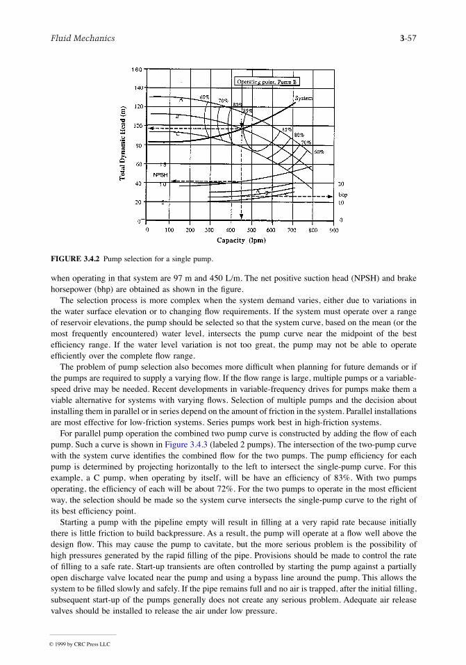
Fluid Mechanics 3-57
when operating in that system are 97 m and 450 L/m. The net positive suction head (NPSH) and brakehorsepower (bhp) are obtained as shown in the Þgure.
The selection process is more complex when the system demand varies, either due to variations inthe water surface elevation or to changing ßow requirements. If the system must operate over a rangeof reservoir elevations, the pump should be selected so that the system curve, based on the mean (or themost frequently encountered) water level, intersects the pump curve near the midpoint of the bestefÞciency range. If the water level variation is not too great, the pump may not be able to operateefÞciently over the complete ßow range.
The problem of pump selection also becomes more difÞcult when planning for future demands or ifthe pumps are required to supply a varying ßow. If the ßow range is large, multiple pumps or a variable-speed drive may be needed. Recent developments in variable-frequency drives for pumps make them aviable alternative for systems with varying ßows. Selection of multiple pumps and the decision aboutinstalling them in parallel or in series depend on the amount of friction in the system. Parallel installationsare most effective for low-friction systems. Series pumps work best in high-friction systems.
For parallel pump operation the combined two pump curve is constructed by adding the ßow of eachpump. Such a curve is shown in Figure 3.4.3 (labeled 2 pumps). The intersection of the two-pump curvewith the system curve identiÞes the combined ßow for the two pumps. The pump efÞciency for eachpump is determined by projecting horizontally to the left to intersect the single-pump curve. For thisexample, a C pump, when operating by itself, will be have an efÞciency of 83%. With two pumpsoperating, the efÞciency of each will be about 72%. For the two pumps to operate in the most efÞcientway, the selection should be made so the system curve intersects the single-pump curve to the right ofits best efÞciency point.
Starting a pump with the pipeline empty will result in Þlling at a very rapid rate because initiallythere is little friction to build backpressure. As a result, the pump will operate at a ßow well above thedesign ßow. This may cause the pump to cavitate, but the more serious problem is the possibility ofhigh pressures generated by the rapid Þlling of the pipe. Provisions should be made to control the rateof Þlling to a safe rate. Start-up transients are often controlled by starting the pump against a partiallyopen discharge valve located near the pump and using a bypass line around the pump. This allows thesystem to be Þlled slowly and safely. If the pipe remains full and no air is trapped, after the initial Þlling,subsequent start-up of the pumps generally does not create any serious problem. Adequate air releasevalves should be installed to release the air under low pressure.
FIGURE 3.4.2 Pump selection for a single pump.
© 1999 by CRC Press LLC
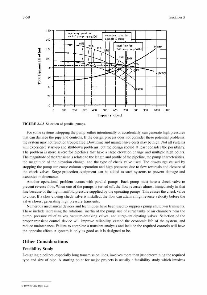
3-58 Section 3
For some systems, stopping the pump, either intentionally or accidentally, can generate high pressuresthat can damage the pipe and controls. If the design process does not consider these potential problems,the system may not function trouble free. Downtime and maintenance costs may be high. Not all systemswill experience start-up and shutdown problems, but the design should at least consider the possibility.The problem is more severe for pipelines that have a large elevation change and multiple high points.The magnitude of the transient is related to the length and proÞle of the pipeline, the pump characteristics,the magnitude of the elevation change, and the type of check valve used. The downsurge caused bystopping the pump can cause column separation and high pressures due to ßow reversals and closure ofthe check valves. Surge-protection equipment can be added to such systems to prevent damage andexcessive maintenance.
Another operational problem occurs with parallel pumps. Each pump must have a check valve toprevent reverse ßow. When one of the pumps is turned off, the ßow reverses almost immediately in thatline because of the high manifold pressure supplied by the operating pumps. This causes the check valveto close. If a slow-closing check valve is installed, the ßow can attain a high reverse velocity before thevalve closes, generating high pressure transients.
Numerous mechanical devices and techniques have been used to suppress pump shutdown transients.These include increasing the rotational inertia of the pump, use of surge tanks or air chambers near thepump, pressure relief valves, vacuum-breaking valves, and surge-anticipating valves. Selection of theproper transient control device will improve reliability, extend the economic life of the system, andreduce maintenance. Failure to complete a transient analysis and include the required controls will havethe opposite effect. A system is only as good as it is designed to be.
Other Considerations
Feasibility Study
Designing pipelines, especially long transmission lines, involves more than just determining the requiredtype and size of pipe. A starting point for major projects is usually a feasibility study which involves
FIGURE 3.4.3 Selection of parallel pumps.
© 1999 by CRC Press LLC
Fluid Mechanics 3-59
social, environmental, political, and legal issues, as well as an economic evaluation of the engineeringalternatives developed during the preliminary design. The preliminary design should identify the scopeof the project and all major features that inßuence the cost or viability. Since local laws, social values,and environmental concerns vary signiÞcantly between geographic areas, the engineer must be awareof the problems unique to the area.
Choices that affect the economics of the project include alternative pipe routes, amount of storageand its effect on reliability and controllability of ßow, choice of pipe material, diameter and pressureclass, provision for future demands, etc. In making decisions one must consider both the engineeringand economic advantages of the alternatives. Reliability, safety, maintenance, operating, and replacementcosts must all be given their proper value. The analysis should consider (1) expected life of the pipe,which is a function of the type of pipe material and the use of linings or protective coatings; (2) economiclife, meaning how long the pipe will supply the demand; (3) planning for future demand; (4) pumpingcost vs. pipe cost; and (5) provisions for storage.
During the feasibility study only a general design has been completed so a detailed analysis of allhydraulic problems and their solutions is not available. Even so, it is necessary to anticipate the needfor special facilities or equipment and problems such as safe Þlling, provisions for draining, cavitationat control valves, and transient problems caused by valve or pump operation. Provisions should be madefor the cost of the detailed analysis, design, and construction costs required to control special operationalproblems. Attention should also be given to costs associated with winterizing, stream crossings, highwayscrossing, special geologic or topographic problems, and any other items that would have a signiÞcantinßuence on the cost, reliability, or safety of the project.
Storage
The purposes of storage tanks and intermediate reservoirs include (1) to supply water when there is atemporary interruption of ßow from the supply, (2) to provide supplemental water during peak periods,(3) to sectionalize the pipe to reduce mean and transient pressures, (4) to maintain pressure (elevatedstorage), and (5) to simplify control. Storage also has a signiÞcant impact on the control structures,pumping plants, and general operation of the pipeline. If there is adequate storage, large ßuctuations indemand can be tolerated. Any mismatch in supply and demand is made up for by an increase or decreasein storage, and valves in the transmission main will require only infrequent adjustments to maintainstorage. Pumps can be activated by level controls at the storage tank and not by ßuctuations in demandso they can operate for long periods near their design point.
If there is no storage, the system may have to provide continuous Þne adjustment of the ßow toprovide the required ßow within safe pressure limits. For gravity systems this may require automaticpressure- or ßow-regulating valves. For pumped systems, the variations in ßow can cause constant-speedcentrifugal pumps to operate both below and above their design point where power consumption is high,efÞciency is low, and where there is more chance of operational problems. Selection of a variable-frequency drive can avoid these problems. The selection of multiple pumps vs. a variable-speed pumpis primarily a economic decision.
Thrust Blocks
Any time there is a change of pipe alignment, an unbalanced force is developed. The force required torestrain the pipe can be calculated with the two-dimensional, steady state momentum equation. Forburied pipelines, this force can be transmitted to the soil with a thrust block. Determining the size ofthe block and, consequently, the bearing surface area depends on pipe diameter, ßuid pressure, deßectionangle of the pipe, and bearing capacity of the soil. A convenient monograph for sizing thrust blocks waspublished in the Civil Engineering in 1969 (Morrison, 1969).
© 1999 by CRC Press LLC
3-60 Section 3
References
ASCE. 1992. Pressure Pipeline Design for Water and Wastewater. Prepared by the Committee on PipelinePlanning of the Pipeline Division of the American Society of Civil Engineers, New York.
Kalsi Engineering and Tullis Engineering Consultants. 1993. Application Guide for Check Valves inNuclear Power Plants, Revision 1, NP-5479. Prepared for Nuclear Maintenance ApplicationsCenter, Charlotte, NC.
Miller, D.S. 1990. Internal Flow Systems Ñ Design and Performance Prediction, 2nd ed. Gulf PublishingCompany, Houston.
Morrison, E.B. 1969. Monograph for the design of thrust blocks. Civil Eng., 39, June, 55Ð51.Spanger, M.G. and Handy, R.L. 1973. Soil Engineering, 3rd ed. Intext Eductational Publishers, New
York, Chap. 25 and 26.Streeter, V.L. and Wylie, E.B. 1975. Fluid Mechanics, 6th ed. McGraw-Hill, New York, 752 pp.Thorley, A.R.D. 1989. Check valve behavior under transient ßow conditions: a state-of-the-art review.
ASME, 111, Vol. 2, June. J. Fluids Engineering: Transactions of the ASME, pp. 173Ð183.Tullis, J.P. 1989. Hydraulics of Pipelines Ñ Pumps, Valves, Cavitation, Transients, John Wiley and Sons,
New York.Tullis, J.P. 1993. Cavitation Guide for Control Valves, NUREG/CR-6031, U.S. Nuclear Regulatory
Commission, Washington, D.C.Wood, D.J. 1966. An explicit friction factor relationship. Civil Eng., 36, December, 60Ð61.Wylie, E.B. and Streeter, V.L. 1993. Fluid Transients in Systems, Prentice-Hall, Englewood Cliffs, N.J.
Further Information
Bean, H.S., ed. 1971. Fluid Meters, Their Theory and Application, 6th ed. The American Society ofMechanical Engineers, New York.Handbook of PVC-Design and Construction. 1979. Uni-Bell Plastic Pipe Association, Dallas.King, H.W. 1954. Handbook of Hydraulics Ñ For the Solution of Hydraulic Problems, 4th ed. Revisedby E.F. Brater. McGraw-Hill, New York.Stephenson, D. 1981. Pipeline Design for Water Engineers, 2nd ed. Elsevier ScientiÞc PublishingCompany, Distributed in the U.S. by Gulf Publishing Company, Houston.Stutsman, R.D. 1993. Steel Penstocks, ASCE Manuals and Reports on Engineering Practice No. 79,Energy Division, American Society of Civil Engineers, New York.Watkins, R.K. and Spangler, M.G., Some Characteristics of the Modulus of Passive Resistance of Soil:A Study in Similitude. Highway Research Board Proceedings Vol. 37, 1958, pp. 576Ð583.Tullis, J.P. 1996. Valves, in Dorf, R.C., Ed., The Engineering Handbook, CRC Press, Boca Raton, FL.
© 1999 by CRC Press LLC
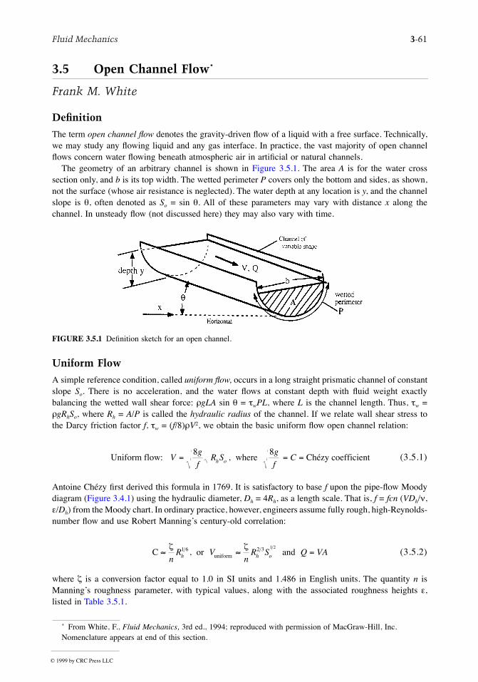
Fluid Mechanics 3-61
3.5 Open Channel Flow*
Frank M. White
Definition
The term open channel ßow denotes the gravity-driven ßow of a liquid with a free surface. Technically,we may study any ßowing liquid and any gas interface. In practice, the vast majority of open channelßows concern water ßowing beneath atmospheric air in artiÞcial or natural channels.
The geometry of an arbitrary channel is shown in Figure 3.5.1. The area A is for the water crosssection only, and b is its top width. The wetted perimeter P covers only the bottom and sides, as shown,not the surface (whose air resistance is neglected). The water depth at any location is y, and the channelslope is q, often denoted as So = sin q. All of these parameters may vary with distance x along thechannel. In unsteady ßow (not discussed here) they may also vary with time.
Uniform Flow
A simple reference condition, called uniform ßow, occurs in a long straight prismatic channel of constantslope So. There is no acceleration, and the water ßows at constant depth with ßuid weight exactlybalancing the wetted wall shear force: rgLA sin q = twPL, where L is the channel length. Thus, tw =rgRhSo, where Rh = A/P is called the hydraulic radius of the channel. If we relate wall shear stress tothe Darcy friction factor f, tw = (f/8)rV2, we obtain the basic uniform ßow open channel relation:
(3.5.1)
Antoine Ch�zy Þrst derived this formula in 1769. It is satisfactory to base f upon the pipe-ßow Moodydiagram (Figure 3.4.1) using the hydraulic diameter, Dh = 4Rh, as a length scale. That is, f = fcn (VDh/n,e/Dh) from the Moody chart. In ordinary practice, however, engineers assume fully rough, high-Reynolds-number ßow and use Robert ManningÕs century-old correlation:
(3.5.2)
where z is a conversion factor equal to 1.0 in SI units and 1.486 in English units. The quantity n isManningÕs roughness parameter, with typical values, along with the associated roughness heights e,listed in Table 3.5.1.
* From White, F., Fluid Mechanics, 3rd ed., 1994; reproduced with permission of MacGraw-Hill, Inc. Nomenclature appears at end of this section.
FIGURE 3.5.1 DeÞnition sketch for an open channel.
Uniform flow: where Ch�zy coefficientVg
fR S
g
fCh o= = =
8 8,
C or anduniform» » =z zn
R Vn
R S Q VAh h o1 6 2 3 1 2
,
© 1999 by CRC Press LLC
3-62 Section 3
Critical Flow
Since the surface is always atmospheric, pressure head is not important in open channel ßows. Totalenergy E relates only to velocity and elevation:
At a given volume ßow rate Q, the energy passes through a minimum at a condition called critical ßow,where dE/dy = 0, or dA/dy = b = gA3/Q2:
(3.5.3)
where b is the top-surface width as in Figure 3.5.1. The velocity Vcrit equals the speed of propagationof a surface wave along the channel. Thus, we may deÞne the Froude number Fr of a channel ßow, forany cross section, as Fr = V/Vcrit. The three regimes of channel ßow are
TABLE 3.5.1 Average Roughness Parameters for Various Channel Surfaces
Average Roughness Height e
n ft mm
ArtiÞcial lined channelsGlass 0.010 ± 0.002 0.0011 0.3Brass 0.011 ± 0.002 0.0019 0.6Steel; smooth 0.012 ± 0.002 0.0032 1.0Painted 0.014 ± 0.003 0.0080 2.4Riveted 0.015 ± 0.002 0.012 3.7
Cast iron 0.013 ± 0.003 0.0051 1.6Cement; Þnished 0.012 ± 0.002 0.0032 1.0UnÞnished 0.014 ± 0.002 0.0080 2.4
Planed wood 0.012 ± 0.002 0.0032 1.0Clay tile 0.014 ± 0.003 0.0080 2.4Brickwork 0.015 ± 0.002 0.012 3.7Asphalt 0.016 ± 0.003 0.018 5.4Corrugated metal 0.022 ± 0.005 0.12 37Rubble masonry 0.025 ± 0.005 0.26 80Excavated earth channelsClean 0.022 ± 0.004 0.12 37Gravelly 0.025 ± 0.005 0.26 80Weedy 0.030 ± 0.005 0.8 240Stony; cobbles 0.035 ± 0.010 1.5 500Natural channelsClean and straight 0.030 ± 0.005 0.8 240Sluggish, deep pools 0.040 ± 0.010 3 900Major rivers 0.035 ± 0.010 1.5 500FloodplainsPasture, farmland 0.035 ± 0.010 1.5 500Light brush 0.05 ± 0.02 6 2000Heavy brush 0.075 ± 0.025 15 5000Trees 0.15 ± 0.05 ? ?
Specific energy E yV
gy
Q
gA= + = +
2 2
22 2
AbQ
gV
Q
A
gA
bcrit critcrit
crit=æ
èç
ö
ø÷ = = æ
èç
öø÷
2 1 3 1 2
Fr < 1: subcritical flow; Fr = 1: critical flow; Fr > 1: supercritical flow
© 1999 by CRC Press LLC
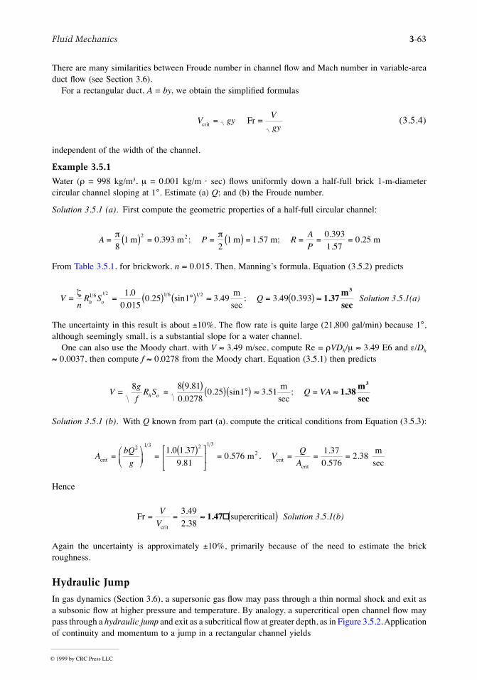
Fluid Mechanics 3-63
There are many similarities between Froude number in channel ßow and Mach number in variable-areaduct ßow (see Section 3.6).
For a rectangular duct, A = by, we obtain the simpliÞed formulas
(3.5.4)
independent of the width of the channel.
Example 3.5.1
Water (r = 998 kg/m3, m = 0.001 kg/m á sec) ßows uniformly down a half-full brick 1-m-diametercircular channel sloping at 1°. Estimate (a) Q; and (b) the Froude number.
Solution 3.5.1 (a). First compute the geometric properties of a half-full circular channel:
From Table 3.5.1, for brickwork, n » 0.015. Then, ManningÕs formula, Equation (3.5.2) predicts
The uncertainty in this result is about ±10%. The ßow rate is quite large (21,800 gal/min) because 1°,although seemingly small, is a substantial slope for a water channel.
One can also use the Moody chart. with V » 3.49 m/sec, compute Re = rVDh/m » 3.49 E6 and e/Dh
» 0.0037, then compute f » 0.0278 from the Moody chart. Equation (3.5.1) then predicts
Solution 3.5.1 (b). With Q known from part (a), compute the critical conditions from Equation (3.5.3):
Hence
Again the uncertainty is approximately ±10%, primarily because of the need to estimate the brickroughness.
Hydraulic Jump
In gas dynamics (Section 3.6), a supersonic gas ßow may pass through a thin normal shock and exit asa subsonic ßow at higher pressure and temperature. By analogy, a supercritical open channel ßow maypass through a hydraulic jump and exit as a subcritical ßow at greater depth, as in Figure 3.5.2. Applicationof continuity and momentum to a jump in a rectangular channel yields
V gyV
gycrit Fr ==
A P RA
P= ( ) = = ( ) = = = =
p p8
1 0 3932
1 1 570 3931 57
0 252
m m m m m2. ; . ;..
.
Vn
R S Qh o=m
secz 1 6 1 6 1 21 2 1 0
0 0150 25 1 3 49 3 49 0 393= ( ) °( ) » = ( ) »
..
. sin . ; . . 1.37msec
3
Solution 3.5.1(a)
Vg
fR S Q VAh o=
msec
8 8 9 81
0 02780 25 1 3 51=
( ) ( ) °( ) » = ».
.. sin . ; 1.38
msec
3
AbQ
gV
Q
Acrit2
critcrit
m m
sec=
æ
èç
ö
ø÷ =
( )é
ëê
ù
ûú = = = =
2 1 3 2 1 31 0 1 37
9 810 576
1 370 576
2 38. .
.. ,
..
.
Fr supercriticalcrit
= = » ( )V
V
3 492 38..
1.47 Solution 3.5.1(b)
© 1999 by CRC Press LLC
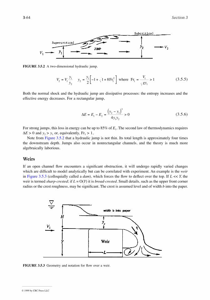
3-64 Section 3
(3.5.5)
Both the normal shock and the hydraulic jump are dissipative processes: the entropy increases and theeffective energy decreases. For a rectangular jump,
(3.5.6)
For strong jumps, this loss in energy can be up to 85% of E1. The second law of thermodynamics requiresDE > 0 and y2 > y1 or, equivalently, Fr1 > 1,
Note from Figure 3.5.2 that a hydraulic jump is not thin. Its total length is approximately four timesthe downstream depth. Jumps also occur in nonrectangular channels, and the theory is much morealgebraically laborious.
Weirs
If an open channel ßow encounters a signiÞcant obstruction, it will undergo rapidly varied changeswhich are difÞcult to model analytically but can be correlated with experiment. An example is the weirin Figure 3.5.3 (colloquially called a dam), which forces the ßow to deßect over the top. If L << Y, theweir is termed sharp-crested; if L = O(Y) it is broad-crested. Small details, such as the upper front cornerradius or the crest roughness, may be signiÞcant. The crest is assumed level and of width b into the paper.
FIGURE 3.5.2 A two-dimensional hydraulic jump.
FIGURE 3.5.3 Geometry and notation for ßow over a weir.
V Vy
yy
y V
gy2 11
22
1 1
121 1 8 1= = - + +[ ] = >Fr where Fr1
21
DE E Ey y
y y= - =
-( )>1 2
2 1
3
1 240
© 1999 by CRC Press LLC
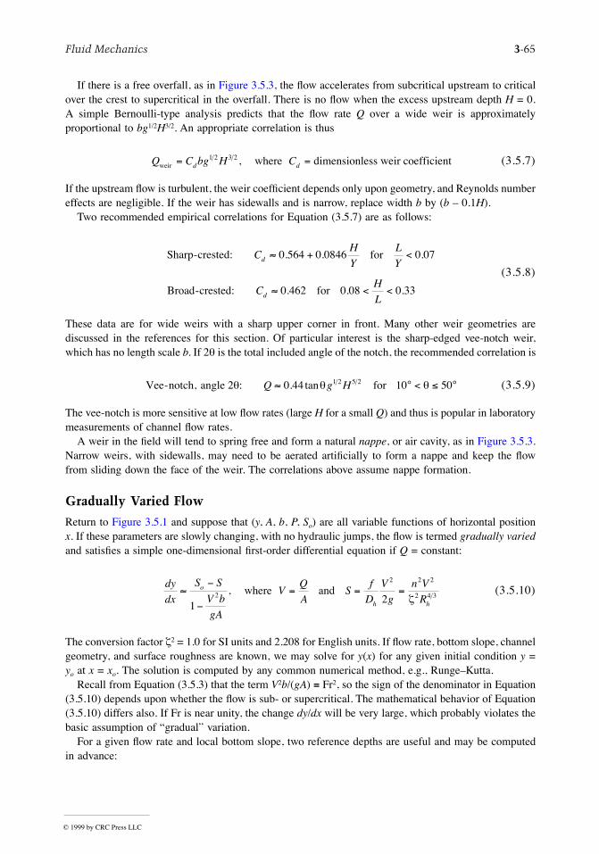
Fluid Mechanics 3-65
If there is a free overfall, as in Figure 3.5.3, the ßow accelerates from subcritical upstream to criticalover the crest to supercritical in the overfall. There is no ßow when the excess upstream depth H = 0.A simple Bernoulli-type analysis predicts that the ßow rate Q over a wide weir is approximatelyproportional to bg1/2H3/2. An appropriate correlation is thus
(3.5.7)
If the upstream ßow is turbulent, the weir coefÞcient depends only upon geometry, and Reynolds numbereffects are negligible. If the weir has sidewalls and is narrow, replace width b by (b Ð 0.1H).
Two recommended empirical correlations for Equation (3.5.7) are as follows:
(3.5.8)
These data are for wide weirs with a sharp upper corner in front. Many other weir geometries arediscussed in the references for this section. Of particular interest is the sharp-edged vee-notch weir,which has no length scale b. If 2q is the total included angle of the notch, the recommended correlation is
(3.5.9)
The vee-notch is more sensitive at low ßow rates (large H for a small Q) and thus is popular in laboratorymeasurements of channel ßow rates.
A weir in the Þeld will tend to spring free and form a natural nappe, or air cavity, as in Figure 3.5.3.Narrow weirs, with sidewalls, may need to be aerated artiÞcially to form a nappe and keep the ßowfrom sliding down the face of the weir. The correlations above assume nappe formation.
Gradually Varied Flow
Return to Figure 3.5.1 and suppose that (y, A, b, P, So) are all variable functions of horizontal positionx. If these parameters are slowly changing, with no hydraulic jumps, the ßow is termed gradually variedand satisÞes a simple one-dimensional Þrst-order differential equation if Q = constant:
(3.5.10)
The conversion factor z2 = 1.0 for SI units and 2.208 for English units. If ßow rate, bottom slope, channelgeometry, and surface roughness are known, we may solve for y(x) for any given initial condition y =yo at x = xo. The solution is computed by any common numerical method, e.g., RungeÐKutta.
Recall from Equation (3.5.3) that the term V2b/(gA) º Fr2, so the sign of the denominator in Equation(3.5.10) depends upon whether the ßow is sub- or supercritical. The mathematical behavior of Equation(3.5.10) differs also. If Fr is near unity, the change dy/dx will be very large, which probably violates thebasic assumption of ÒgradualÓ variation.
For a given ßow rate and local bottom slope, two reference depths are useful and may be computedin advance:
Q C bg H Cd dweir where dimensionless weir coefficient= =1 2 3 2 ,
Sharp-crested: for
Broad-crested: for
CH
Y
L
Y
CH
L
d
d
» + <
» < <
0 564 0 0846 0 07
0 462 0 08 0 33
. . .
. . .
Vee-notch, angle 2 : forq q qQ g H» ° < £ °0 44 10 501 2 5 2. tan
dy
dx
S S
V b
gA
VQ
AS
f
D
V
g
n V
Ro
h h
»-
-= = =
122
2 2 2
2 4 3, where andz
© 1999 by CRC Press LLC
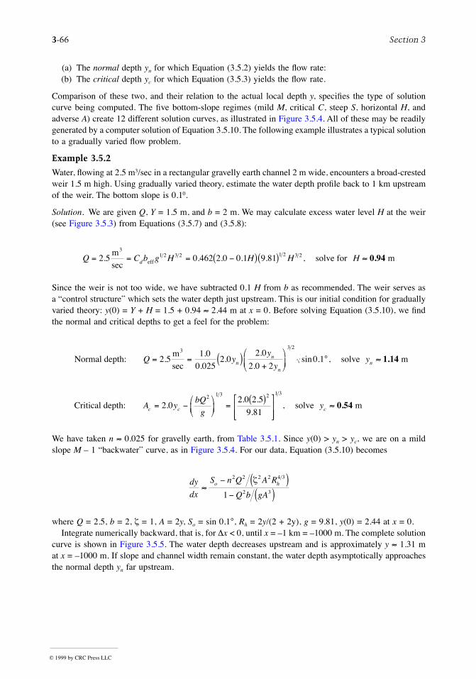
3-66 Section 3
(a) The normal depth yn for which Equation (3.5.2) yields the ßow rate:(b) The critical depth yc for which Equation (3.5.3) yields the ßow rate.
Comparison of these two, and their relation to the actual local depth y, speciÞes the type of solutioncurve being computed. The Þve bottom-slope regimes (mild M, critical C, steep S, horizontal H, andadverse A) create 12 different solution curves, as illustrated in Figure 3.5.4. All of these may be readilygenerated by a computer solution of Equation 3.5.10. The following example illustrates a typical solutionto a gradually varied ßow problem.
Example 3.5.2
Water, ßowing at 2.5 m3/sec in a rectangular gravelly earth channel 2 m wide, encounters a broad-crestedweir 1.5 m high. Using gradually varied theory, estimate the water depth proÞle back to 1 km upstreamof the weir. The bottom slope is 0.10.
Solution. We are given Q, Y = 1.5 m, and b = 2 m. We may calculate excess water level H at the weir(see Figure 3.5.3) from Equations (3.5.7) and (3.5.8):
Since the weir is not too wide, we have subtracted 0.1 H from b as recommended. The weir serves asa Òcontrol structureÓ which sets the water depth just upstream. This is our initial condition for graduallyvaried theory: y(0) = Y + H = 1.5 + 0.94 » 2.44 m at x = 0. Before solving Equation (3.5.10), we Þndthe normal and critical depths to get a feel for the problem:
We have taken n » 0.025 for gravelly earth, from Table 3.5.1. Since y(0) > yn > yc, we are on a mildslope M Ð 1 ÒbackwaterÓ curve, as in Figure 3.5.4. For our data, Equation (3.5.10) becomes
where Q = 2.5, b = 2, z = 1, A = 2y, So = sin 0.1°, Rh = 2y/(2 + 2y), g = 9.81, y(0) = 2.44 at x = 0.Integrate numerically backward, that is, for Dx < 0, until x = Ð1 km = Ð1000 m. The complete solution
curve is shown in Figure 3.5.5. The water depth decreases upstream and is approximately y » 1.31 mat x = Ð1000 m. If slope and channel width remain constant, the water depth asymptotically approachesthe normal depth yn far upstream.
Q C b g H H H Hd= = = -( )( ) »2 5 0 462 2 0 0 1 9 811 2 3 2 1 2 3 2.sec
. . . . ,m
solve for m3
eff 0.94
Normal depth:m
solve m3
Q yy
yyn
n
nn= = ( )
+
æ
èç
ö
ø÷ ° »2 5
1 00 025
2 02 0
2 0 20 1
3 2
.sec
..
..
.sin . , 1.14
Critical depth: solve mA ybQ
gyc c c= -
æ
èç
ö
ø÷ =
( )é
ëêê
ù
ûúú
»2 02 0 2 5
9 81
2 1 3 2 1 3
.. .
., 0.54
dy
dx
S n Q A R
Q b gAo h»
- ( )- ( )
2 2 2 2 4 3
2 31
z
© 1999 by CRC Press LLC
Fluid Mechanics 3-67
FIGURE 3.5.4 ClassiÞcation of solution curves for gradually varied ßow.
© 1999 by CRC Press LLC
3-68 Section 3
Nomenclature
English symbols
A = water cross section areab = channel upper-surface widthC = Ch�zy coefÞcient, Equation (3.5.1)
Cd = weir discharge coefÞcient, Equation (3.5.7)Dh = hydraulic diameter, = 4RhE = speciÞc energy, = y + V2/2gf = Moody friction factor
Fr = Froude number, = V/Vcritg = acceleration of gravityH = excess water level above weir, Figure 3.5.3L = weir length, Figure 3.5.3n = Manning roughness factor, Table 3.5.1P = wetted perimeterQ = volume ßow rateRh = hydraulic radius, = A/PS = frictional slope, Equation (3.5.10)
So = bottom slopeV = average velocityx = horizontal distance along the channely = water depthY = weir height, Figure (3.5.3
Greek Symbols
e = wall roughness height, Table 3.5.1r = ßuid densitym = ßuid viscosityn = ßuid kinematic viscosity, = m/rz = conversion factor, = 1.0 (SI) and 1.486 (English)
Subscripts
c,crit = critical, at Fr = 1n = normal, in uniform ßow
FIGURE 3.5.5 Backwater solution curve for Example 3.5.2.
© 1999 by CRC Press LLC
Fluid Mechanics 3-69
References
Ackers, P. et al. 1978. Weirs and Flumes for Flow Measurement, John Wiley, New York.Bos, M.G. 1985. Long-Throated Flumes and Broad-Crested Weirs, Martinus Nijhoff (Kluwer), Dor-
drecht, The Netherlands.Bos, M.G., Replogle, J.A., and Clemmens, A.J. 1984. Flow-Measuring Flumes for Open Channel
Systems, John Wiley, New York.Brater, E.F. 1976. Handbook of Hydraulics, 6th ed., McGraw-Hill, New York.Chow, V.T. 1959. Open Channel Hydraulics, McGraw-Hill, New York.French, R.H. 1985. Open Channel Hydraulics, McGraw-Hill, New York.Henderson, F.M. 1966. Open Channel Flow, Macmillan, New York.Sellin, R.H.J. 1970. Flow in Channels, Gordon & Breach, London.Spitzer, D.W. (Ed.). 1991. Flow Measurement: Practical Guides for Measurement and Control, Instru-
ment Society of America, Research Triangle Park, NC.
© 1999 by CRC Press LLC
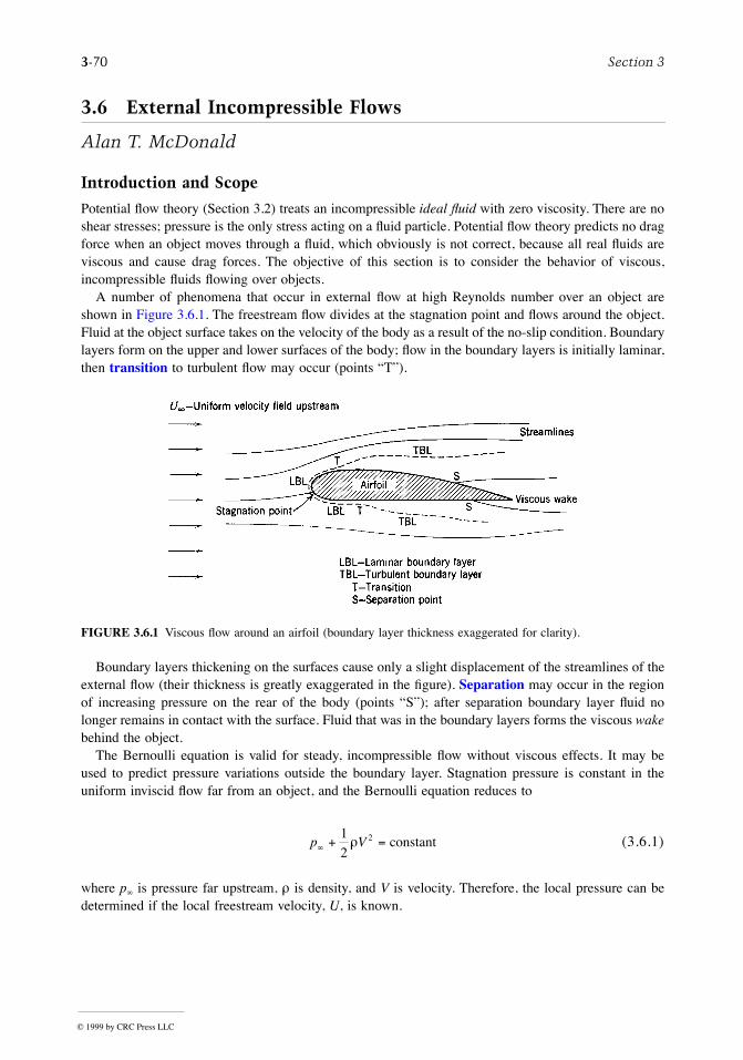
3-70 Section 3
3.6 External Incompressible Flows
Alan T. McDonald
Introduction and Scope
Potential ßow theory (Section 3.2) treats an incompressible ideal ßuid with zero viscosity. There are noshear stresses; pressure is the only stress acting on a ßuid particle. Potential ßow theory predicts no dragforce when an object moves through a ßuid, which obviously is not correct, because all real ßuids areviscous and cause drag forces. The objective of this section is to consider the behavior of viscous,incompressible ßuids ßowing over objects.
A number of phenomena that occur in external ßow at high Reynolds number over an object areshown in Figure 3.6.1. The freestream ßow divides at the stagnation point and ßows around the object.Fluid at the object surface takes on the velocity of the body as a result of the no-slip condition. Boundarylayers form on the upper and lower surfaces of the body; ßow in the boundary layers is initially laminar,then transition to turbulent ßow may occur (points ÒTÓ).
Boundary layers thickening on the surfaces cause only a slight displacement of the streamlines of theexternal ßow (their thickness is greatly exaggerated in the Þgure). Separation may occur in the regionof increasing pressure on the rear of the body (points ÒSÓ); after separation boundary layer ßuid nolonger remains in contact with the surface. Fluid that was in the boundary layers forms the viscous wakebehind the object.
The Bernoulli equation is valid for steady, incompressible ßow without viscous effects. It may beused to predict pressure variations outside the boundary layer. Stagnation pressure is constant in theuniform inviscid ßow far from an object, and the Bernoulli equation reduces to
(3.6.1)
where p¥ is pressure far upstream, r is density, and V is velocity. Therefore, the local pressure can bedetermined if the local freestream velocity, U, is known.
FIGURE 3.6.1 Viscous ßow around an airfoil (boundary layer thickness exaggerated for clarity).
p V¥ + =12
2r constant
© 1999 by CRC Press LLC
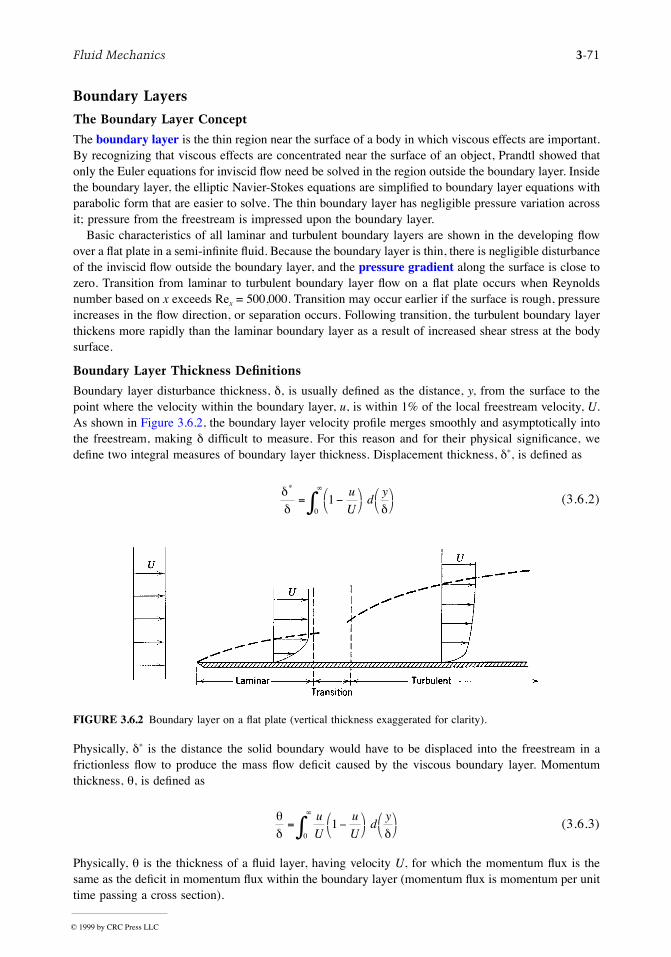
Fluid Mechanics 3-71
Boundary Layers
The Boundary Layer Concept
The boundary layer is the thin region near the surface of a body in which viscous effects are important.By recognizing that viscous effects are concentrated near the surface of an object, Prandtl showed thatonly the Euler equations for inviscid ßow need be solved in the region outside the boundary layer. Insidethe boundary layer, the elliptic Navier-Stokes equations are simpliÞed to boundary layer equations withparabolic form that are easier to solve. The thin boundary layer has negligible pressure variation acrossit; pressure from the freestream is impressed upon the boundary layer.
Basic characteristics of all laminar and turbulent boundary layers are shown in the developing ßowover a ßat plate in a semi-inÞnite ßuid. Because the boundary layer is thin, there is negligible disturbanceof the inviscid ßow outside the boundary layer, and the pressure gradient along the surface is close tozero. Transition from laminar to turbulent boundary layer ßow on a ßat plate occurs when Reynoldsnumber based on x exceeds Rex = 500,000. Transition may occur earlier if the surface is rough, pressureincreases in the ßow direction, or separation occurs. Following transition, the turbulent boundary layerthickens more rapidly than the laminar boundary layer as a result of increased shear stress at the bodysurface.
Boundary Layer Thickness Definitions
Boundary layer disturbance thickness, d, is usually deÞned as the distance, y, from the surface to thepoint where the velocity within the boundary layer, u, is within 1% of the local freestream velocity, U.As shown in Figure 3.6.2, the boundary layer velocity proÞle merges smoothly and asymptotically intothe freestream, making d difÞcult to measure. For this reason and for their physical signiÞcance, wedeÞne two integral measures of boundary layer thickness. Displacement thickness, d*, is deÞned as
(3.6.2)
Physically, d* is the distance the solid boundary would have to be displaced into the freestream in africtionless ßow to produce the mass ßow deÞcit caused by the viscous boundary layer. Momentumthickness, q, is deÞned as
(3.6.3)
Physically, q is the thickness of a ßuid layer, having velocity U, for which the momentum ßux is thesame as the deÞcit in momentum ßux within the boundary layer (momentum ßux is momentum per unittime passing a cross section).
FIGURE 3.6.2 Boundary layer on a ßat plate (vertical thickness exaggerated for clarity).
dd d
*
= -æè
öø
æè
öø
¥
ò01
u
Ud
y
qd d
= -æè
öø
æè
öø
¥
ò01
u
U
u
Ud
y
© 1999 by CRC Press LLC
3-72 Section 3
Because d* and q are deÞned in terms of integrals for which the integrand vanishes in the freestream,they are easier to evaluate experimentally than disturbance thickness d.
Exact Solution of the Laminar Flat-Plate Boundary Layer
Blasius obtained an exact solution for laminar boundary layer ßow on a ßat plate. He assumed a thinboundary layer to simplify the streamwise momentum equation. He also assumed similar velocity proÞlesin the boundary layer, so that when written as u/U = f(y/d), velocity proÞles do not vary with x. He useda similarity variable to reduce the partial differential equations of motion and continuity to a single third-order ordinary differential equation.
Blasius used numerical methods to solve the ordinary differential equation. Unfortunately, the velocityproÞle must be expressed in tabular form. The principal results of the Blasius solution may be expressed as
(3.6.4)
and
(3.6.5)
These results characterize the laminar boundary layer on a ßat plate; they show that laminar boundarylayer thickness varies as x1/2 and wall shear stress varies as 1/x1/2.
Approximate Solutions
The Blasius solution cannot be expressed in closed form and is limited to laminar ßow. Therefore,approximate methods that give solutions for both laminar and turbulent ßow in closed form are desirable.One such method is the momentum integral equation (MIE), which may be developed by integratingthe boundary layer equation across the boundary layer or by applying the streamwise momentum equationto a differential control volume (Fox and McDonald, 1992). The result is the ordinary differential equation
(3.6.6)
The Þrst term on the right side of Equation (3.6.6) contains the inßuence of wall shear stress. Since tw
is always positive, it always causes q to increase. The second term on the right side contains the pressuregradient, which can have either sign. Therefore, the effect of the pressure gradient can be to eitherincrease or decrease the rate of growth of boundary layer thickness.
Equation (3.6.6) is an ordinary differential equation that can be solved for q as a function of x on aßat plate (zero pressure gradient), provided a reasonable shape is assumed for the boundary layer velocityproÞle and shear stress is expressed in terms of the other variables. Results for laminar and turbulentßat-plate boundary layer ßows are discussed below.
Laminar Boundary Layers. A reasonable approximation to the laminar boundary layer velocity proÞleis to express u as a polynomial in y. The resulting solutions for d and tw have the same dependence onx as the exact Blasius solution. Numerical results are presented in Table 3.6.1. Comparing the approximateand exact solutions shows remarkable agreement in view of the approximations used in the analysis.The trends are predicted correctly and the approximate values are within 10% of the exact values.
Turbulent Boundary Layers. The turbulent velocity proÞle may be expressed well using a power law,u/U = (y/d)1/n, where n is an integer between 6 and 10 (frequently 7 is chosen). For turbulent ßow it is
dx x
=5
Re
CU
fw
x
= =t
r12
0 6642
.
Re
d
dx U U
dU
dxwq t
rdq
q= - +
æ
èç
ö
ø÷2 2
*
© 1999 by CRC Press LLC
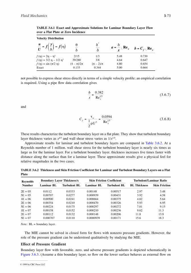
Fluid Mechanics 3-73
not possible to express shear stress directly in terms of a simple velocity proÞle; an empirical correlationis required. Using a pipe ßow data correlation gives
(3.6.7)
and
(3.6.8)
These results characterize the turbulent boundary layer on a ßat plate. They show that turbulent boundarylayer thickness varies as x4/5 and wall shear stress varies as 1/x1/5.
Approximate results for laminar and turbulent boundary layers are compared in Table 3.6.2. At aReynolds number of 1 million, wall shear stress for the turbulent boundary layer is nearly six times aslarge as for the laminar layer. For a turbulent boundary layer, thickness increases Þve times faster withdistance along the surface than for a laminar layer. These approximate results give a physical feel forrelative magnitudes in the two cases.
The MIE cannot be solved in closed form for ßows with nonzero pressure gradients. However, therole of the pressure gradient can be understood qualitatively by studying the MIE.
Effect of Pressure Gradient
Boundary layer ßow with favorable, zero, and adverse pressure gradients is depicted schematically inFigure 3.6.3. (Assume a thin boundary layer, so ßow on the lower surface behaves as external ßow on
TABLE 3.6.1 Exact and Approximate Solutions for Laminar Boundary Layer Flow over a Flat Plate at Zero Incidence
Velocity Distribution
f (h) = 2h Ð h2 2/15 1/3 5.48 0.730f (h) = 3/2 h Ð 1/2 h3 39/280 3/8 4.64 0.647f (h) = sin (p/2 h) (4 Ð p)/2p (p Ð 2)/p 4.80 0.654Exact 0.133 0.344 5.00 0.664
TABLE 3.6.2 Thickness and Skin Friction CoefÞcient for Laminar and Turbulent Boundary Layers on a Flat Plate
Reynolds Number
Boundary Layer Thickness/x Skin Friction CoefÞcient Turbulent/Laminar Ratio
Laminar BL Turbulent BL Laminar BL Turbulent BL BL Thickness Skin Friction
2E + 05 0.0112 0.0333 0.00148 0.00517 2.97 3.485E + 05 0.00707 0.0277 0.000939 0.00431 3.92 4.581E + 06 0.00500 0.0241 0.000664 0.00375 4.82 5.642E + 06 0.00354 0.0210 0.000470 0.00326 5.93 6.955E + 06 0.00224 0.0175 0.000297 0.00272 7.81 9.151E + 07 0.00158 0.0152 0.000210 0.00236 9.62 11.32E + 07 0.00112 0.0132 0.000148 0.00206 11.8 13.95E + 07 0.000707 0.0110 0.0000939 0.00171 15.6 18.3
Note: BL = boundary layer.
uU
fy
f= æèç
öø÷ = ( )
dh q
d
dd
*
ax x=dRe b Cf x= Re
dx x
=0 382
1 5
.Re
CU
fw
x
= =t
r12
0 05942
1 5
.Re
© 1999 by CRC Press LLC
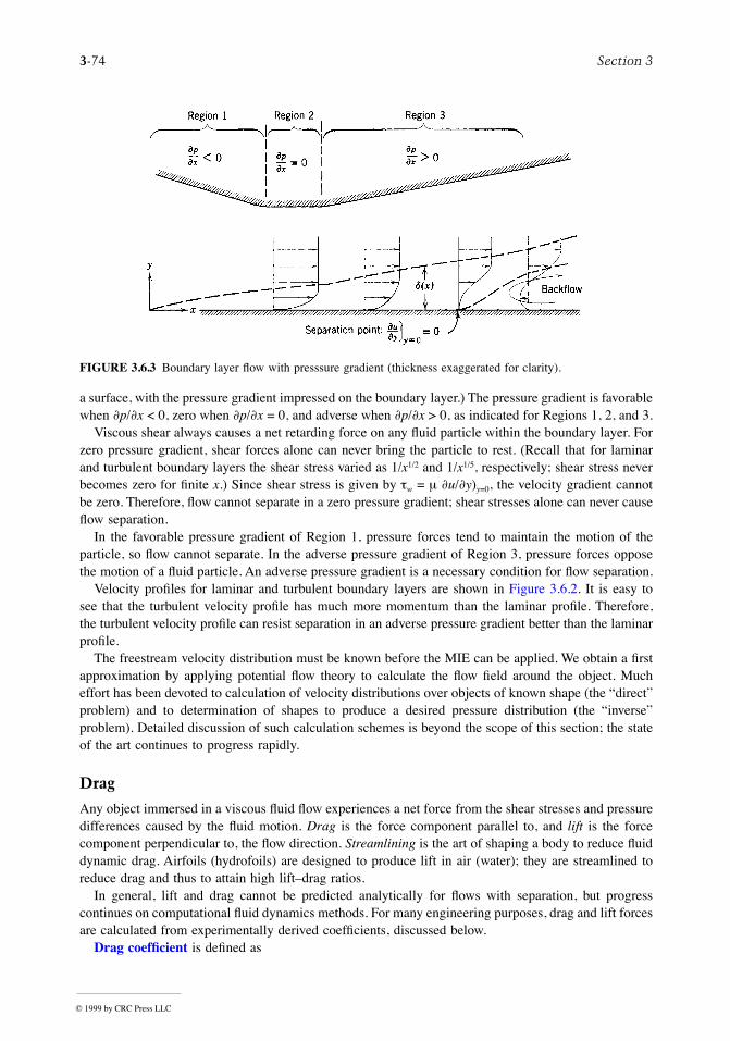
3-74 Section 3
a surface, with the pressure gradient impressed on the boundary layer.) The pressure gradient is favorablewhen ¶p/¶x < 0, zero when ¶p/¶x = 0, and adverse when ¶p/¶x > 0, as indicated for Regions 1, 2, and 3.
Viscous shear always causes a net retarding force on any ßuid particle within the boundary layer. Forzero pressure gradient, shear forces alone can never bring the particle to rest. (Recall that for laminarand turbulent boundary layers the shear stress varied as 1/x1/2 and 1/x1/5, respectively; shear stress neverbecomes zero for Þnite x.) Since shear stress is given by tw = m ¶u/¶y)y=0, the velocity gradient cannotbe zero. Therefore, ßow cannot separate in a zero pressure gradient; shear stresses alone can never causeßow separation.
In the favorable pressure gradient of Region 1, pressure forces tend to maintain the motion of theparticle, so ßow cannot separate. In the adverse pressure gradient of Region 3, pressure forces opposethe motion of a ßuid particle. An adverse pressure gradient is a necessary condition for ßow separation.
Velocity proÞles for laminar and turbulent boundary layers are shown in Figure 3.6.2. It is easy tosee that the turbulent velocity proÞle has much more momentum than the laminar proÞle. Therefore,the turbulent velocity proÞle can resist separation in an adverse pressure gradient better than the laminarproÞle.
The freestream velocity distribution must be known before the MIE can be applied. We obtain a Þrstapproximation by applying potential ßow theory to calculate the ßow Þeld around the object. Mucheffort has been devoted to calculation of velocity distributions over objects of known shape (the ÒdirectÓproblem) and to determination of shapes to produce a desired pressure distribution (the ÒinverseÓproblem). Detailed discussion of such calculation schemes is beyond the scope of this section; the stateof the art continues to progress rapidly.
Drag
Any object immersed in a viscous ßuid ßow experiences a net force from the shear stresses and pressuredifferences caused by the ßuid motion. Drag is the force component parallel to, and lift is the forcecomponent perpendicular to, the ßow direction. Streamlining is the art of shaping a body to reduce ßuiddynamic drag. Airfoils (hydrofoils) are designed to produce lift in air (water); they are streamlined toreduce drag and thus to attain high liftÐdrag ratios.
In general, lift and drag cannot be predicted analytically for ßows with separation, but progresscontinues on computational ßuid dynamics methods. For many engineering purposes, drag and lift forcesare calculated from experimentally derived coefÞcients, discussed below.
Drag coefÞcient is deÞned as
FIGURE 3.6.3 Boundary layer ßow with presssure gradient (thickness exaggerated for clarity).
© 1999 by CRC Press LLC

Fluid Mechanics 3-75
(3.6.9)
where 1/2rV2 is dynamic pressure and A is the area upon which the coefÞcient is based. Common practiceis to base drag coefÞcients on projected frontal area (Fox and McDonald, 1992).
Similitude was treated in Section 3.3. In general, the drag coefÞcient may be expressed as a functionof Reynolds number, Mach number, Froude number, relative roughness, submergence divided by length,and so forth. In this section we consider neither high-speed ßow nor free-surface effects, so we willconsider only Reynolds number and roughness effects on drag coefÞcient.
Friction Drag
The total friction drag force acting on a plane surface aligned with the ßow direction can be found byintegrating the shear stress distribution along the surface. The drag coefÞcient for this case is deÞnedas friction force divided by dynamic pressure and wetted area in contact with the ßuid. Since shearstress is a function of Reynolds number, so is drag coefÞcient (see Figure 3.6.4). In Figure 3.6.4, transitionoccurs at Rex = 500,000; the dashed line represents the drag coefÞcient at larger Reynolds numbers. Anumber of empirical correlations may be used to model the variation in CD shown in Figure 3.6.4(Schlichting, 1979).
Extending the laminar boundary layer line to higher Reynolds numbers shows that it is beneÞcial todelay transition to the highest possible Reynolds number. Some results are presented in Table 3.6.3; dragis reduced more than 50% by extending laminar boundary layer ßow to ReL = 106.
Pressure Drag
A thin ßat surface normal to the ßow has no area parallel to the ßow direction. Therefore, there can beno friction force parallel to the ßow; all drag is caused by pressure forces. Drag coefÞcients for objectswith sharp edges tend to be independent of Reynolds number (for Re > 1000), because the separationpoints are Þxed by the geometry of the object. Drag coefÞcients for selected objects are shown in Table3.6.4.
Rounding the edges that face the ßow reduces drag markedly. Compare the drag coefÞcients for thehemisphere and C-section shapes facing into and away from the ßow. Also note that the drag coefÞcient
FIGURE 3.6.4 Drag coefÞcient vs. Reynolds number for a smooth ßat plate parallel to the ßow.
CF
V AD
D= 12
2r
© 1999 by CRC Press LLC
3-76 Section 3
for a two-dimensional object (long square cylinder) is about twice that for the corresponding three-dimensional object (square cylinder with b/h = 1).
TABLE 3.6.3 Drag CoefÞcients for Laminar, Turbulent, and Transition Boundary Layers on a Flat Plate
Reynolds Number
Drag CoefÞcient Laminar/Transition
% Drag ReductionLaminar BL Turbulent BL Transition
2E + 05 0.00297 0.00615 Ñ Ñ Ñ5E + 05 0.00188 0.00511 0.00189 Ñ Ñ1E + 06 0.00133 0.00447 0.00286 0.464 53.62E + 06 0.000939 0.00394 0.00314 0.300 70.05E + 06 0.000594 0.00336 0.00304 0.195 80.51E + 07 0.000420 0.00300 0.00284 0.148 85.22E + 07 0.000297 0.00269 0.00261 0.114 88.65E + 07 0.000188 0.00235 0.00232 0.081 9.19
Note: BL = Boundary layer.
TABLE 3.6.4 Drag CoefÞcient Data for Selected Objects (Re > 1000)
Object Diagram CD(RE* 103)
Square prism b/h = ¥ 2.05
Disk
b/h = 1 1.05
1.17
Ring 1.20b
Hemisphere (open end facing ßow) 1.42
Hemisphere (open end facing downstream) 0.38
C-section (open side facing ßow) 2.30
C-section (open side facing downstream) 1.20
a Data from Hoerner, 1965.b Based on ring area.
>~
© 1999 by CRC Press LLC
Fluid Mechanics 3-77
Friction and Pressure Drag: Bluff Bodies
Both friction and pressure forces contribute to the drag of bluff bodies (see Shapiro, 1960, for a gooddiscussion of the mechanisms of drag). As an example, consider the drag coefÞcient for a smooth sphereshown in Figure 3.6.5. Transition from laminar to turbulent ßow in the boundary layers on the forwardportion of the sphere causes a dramatic dip in drag coefÞcient at the critical Reynolds number (ReD »2 ´ 105). The turbulent boundary layer is better able to resist the adverse pressure gradient on the rearof the sphere, so separation is delayed and the wake is smaller, causing less pressure drag.
Surface roughness (or freestream disturbances) can reduce the critical Reynolds number. Dimples ona golf ball cause the boundary layer to become turbulent and, therefore, lower the drag coefÞcient inthe range of speeds encountered in a drive.
Streamlining
Streamlining is adding a faired tail section to reduce the extent of separated ßow on the downstreamportion of an object (at high Reynolds number where pressure forces dominate drag). The adversepressure gradient is taken over a longer distance, delaying separation. However, adding a faired tailincreases surface area, causing skin friction drag to increase. Thus, streamlining must be optimized foreach shape.
Front contours are of principal importance in road vehicle design; the angle of the back glass also isimportant (in most cases the entire rear end cannot be made long enough to control separation and reducedrag signiÞcantly).
Lift
Lift coefÞcient is deÞned as
(3.6.10)
Note that lift coefÞcient is based on projected planform area.
FIGURE 3.6.5 Drag coefÞcient vs. Reynolds number for a smooth sphere.
400
100 101 102 103 104 105 1060.06
100
10
1
0.01
CD
Re = VDv
CF
V AL
L= 12
2r
© 1999 by CRC Press LLC
3-78 Section 3
Airfoils
Airfoils are shaped to produce lift efÞciently by accelerating ßow over the upper surface to produce alow-pressure region. Because the ßow must again decelerate, inevitably there must be a region of adversepressure gradient near the rear of the upper surface (pressure distributions are shown clearly in Hazen,1965).
Lift and drag coefÞcients for airfoil sections depend on Reynolds number and angle of attack betweenthe chord line and the undisturbed ßow direction. The chord line is the straight line joining the leadingand trailing edges of the airfoil (Abbott and von Doenhoff, 1959).
As the angle of attack is increased, the minimum pressure point moves forward on the upper surfaceand the minimum pressure becomes lower. This increases the adverse pressure gradient. At some angleof attack, the adverse pressure gradient is strong enough to cause the boundary layer to separatecompletely from the upper surface, causing the airfoil to stall. The separated ßow alters the pressuredistribution, reducing lift sharply.
Increasing the angle of attack also causes the the drag coefÞcient to increase. At some angle of attackbelow stall the ratio of lift to drag, the liftÐdrag ratio, reaches a maximum value.
Drag Due to Lift
For wings (airfoils of Þnite span), lift and drag also are functions of aspect ratio. Lift is reduced anddrag increased compared with inÞnite span, because end effects cause the lift vector to rotate rearward.For a given geometric angle of attack, this reduces effective angle of attack, reducing lift. The additionalcomponent of lift acting in the ßow direction increases drag; the increase in drag due to lift is calledinduced drag.
The effective aspect ratio includes the effect of planform shape. When written in terms of effectiveaspect ratio, the drag of a Þnite-span wing is
(3.6.11)
where ar is effective aspect ratio and the subscript ¥ refers to the inÞnite section drag coefÞcient at CL.For further details consult the references.
The lift coefÞcient must increase to support aircraft weight as speed is reduced. Therefore, induceddrag can increase rapidly at low ßight speeds. For this reason, minimum allowable ßight speeds forcommercial aircraft are closely controlled by the FAA.
Boundary Layer Control
The major part of the drag on an airfoil or wing is caused by skin friction. Therefore, it is important tomaintain laminar ßow in the boundary layers as far aft as possible; laminar ßow sections are designedto do this. It also is important to prevent ßow separation and to achieve high lift to reduce takeoff andlanding speeds. These topics fall under the general heading of boundary layer control.
Profile Shaping
Boundary layer transition on a conventional airfoil section occurs almost immediately after the minimumpressure at about 25% chord aft the leading edge. Transition can be delayed by shaping the proÞle tomaintain a favorable pressure gradient over more of its length. The U.S. National Advisory Committeefor Aeronautics (NACA) developed several series of proÞles that delayed transition to 60 or 65% ofchord, reducing drag coefÞcients (in the design range) 60% compared with conventional sections of thesame thickness ratio (Abbott and von Doenhoff, 1959).
C CC
arD DL= +¥,
2
p
© 1999 by CRC Press LLC
Fluid Mechanics 3-79
Flaps and Slats
Flaps are movable sections near the trailing edge of a wing. They extend and/or deßect to increase wingarea and/or increase wing camber (curvature), to provide higher lift than the clean wing. Many aircraftalso are Þtted with leading edge slats which open to expose a slot from the pressure side of the wingto the upper surface. The open slat increases the effective radius of the leading edge, improving maximumlift coefÞcient. The slot allows energized air from the pressure surface to ßow into the low-pressureregion atop the wing, energizing the boundary layers and delaying separation and stall.
Suction and Blowing
Suction removes low-energy ßuid from the boundary layer, reducing the tendency for early separation.Blowing via high-speed jets directed along the surface reenergizes low-speed boundary layer ßuid. Theobjective of both approaches is to delay separation, thus increasing the maximum lift coefÞcient thewing can achieve. Powered systems add weight and complexity; they also require bleed air from theengine compressor, reducing thrust or power output.
Moving Surfaces
Many schemes have been proposed to utilize moving surfaces for boundary layer control. Motion in thedirection of ßow reduces skin friction, and thus the tendency to separate; motion against the ßow hasthe opposite effect. The aerodynamic behavior of sports balls Ñ baseballs, golf balls, and tennis ballsÑ depends signiÞcantly on aerodynamic side force (lift, down force, or side force) produced by spin.These effects are discussed at length in Fox and McDonald (1992) and its references.
Computation vs. Experiment
Experiments cannot yet be replaced completely by analysis. Progress in modeling, numerical techniques,and computer power continues to be made, but the role of the experimentalist likely will remain importantfor the foreseeable future.
Computational Fluid Dynamics (CFD)
Computation of ßuid ßow requires accurate mathematical modeling of ßow physics and accurate numer-ical procedures to solve the equations. The basic equations for laminar boundary layer ßow are wellknown. For turbulent boundary layers generally it is not possible to resolve the solution space intosufÞciently small cells to allow direct numerical simulation. Instead, empirical models for the turbulentstresses must be used. Advances in computer memory storage capacity and speed (e.g., through use ofmassively parallel processing) continue to increase the resolution that can be achieved.
A second source of error in CFD work results from the numerical procedures required to solve theequations. Even if the equations are exact, approximations must be made to discretize and solve themusing Þnite-difference or Þnite-volume methods. Whichever is chosen, the solver must guard againstintroducing numerical instability, round-off errors, and numerical diffusion (Hoffman, 1992).
Role of the Wind Tunnel
Traditionally, wind tunnel experiments have been conducted to verify the design and performance ofcomponents and complete aircraft. Design veriÞcation of a modern aircraft may require expensive scalemodels, several thousand hours of wind tunnel time at many thousands of dollars an hour, and additionalfull-scale ßight testing.
New wind tunnel facilities continue to be built and old ones refurbished. This indicates a need forcontinued experimental work in developing and optimizing aircraft conÞgurations.
Many experiments are designed to produce baseline data to validate computer codes. Such systematicexperimental data can help to identify the strengths and weaknesses of computational methods.
CFD tends to become only indicative of trends when massive zones of ßow separation are present.Takeoff and landing conÞgurations of conventional aircraft, with landing gear, high-lift devices, and
© 1999 by CRC Press LLC
3-80 Section 3
ßaps extended, tend to need Þnal experimental conÞrmation and optimization. Many studies of verticaltakeoff and vectored thrust aircraft require testing in wind tunnels.
Defining Terms
Boundary layer: Thin layer of ßuid adjacent to a surface where viscous effects are important; viscouseffects are negligible outside the boundary layer.
Drag coefÞcient: Force in the ßow direction exerted on an object by the ßuid ßowing around it, dividedby dynamic pressure and area.
Lift coefÞcient: Force perpendicular to the ßow direction exerted on an object by the ßuid ßowingaround it, divided by dynamic pressure and area.
Pressure gradient: Variation in pressure along the surface of an object. For a favorable pressure gradient,pressure decreases in the ßow direction; for an adverse pressure gradient, pressure increases inthe ßow direction.
Separation: Phenomenon that occurs when ßuid layers adjacent to a solid surface are brought to restand boundary layers depart from the surface contour, forming a low-pressure wake region. Sepa-ration can occur only in an adverse pressure gradient.
Transition: Change from laminar to turbulent ßow within the boundary layer. The location depends ondistance over which the boundary layer has developed, pressure gradient, surface roughness,freestream disturbances, and heat transfer.
References
Abbott, I.H. and von Doenhoff, A.E. 1959. Theory of Wing Sections, Including a Summary of AirfoilData. Dover, New York.
Fox, R.W. and McDonald, A.T. 1992. Introduction to Fluid Mechanics, 4th ed. John Wiley & Sons, NewYork.
Hazen, D.C. 1965. Boundary Layer Control, Þlm developed by the National Committee for FluidMechanics Films (NCFMF) and available on videotape from Encyclopaedia Britannica EducationalCorporation, Chicago.
Hoerner, S.F. 1965. Fluid-Dynamic Drag, 2nd ed. Published by the author, Midland Park, NJ.Hoffman, J.D. 1992. Numerical Methods for Engineers and Scientists. McGraw-Hill, New York.Schlichting, H. 1979. Boundary-Layer Theory, 7th ed. McGraw-Hill, New York.Shapiro, A.H. 1960. The Fluid Dynamics of Drag, Þlm developed by the National Committee for Fluid
Mechanics Film (NCFMF) and available on videotape from Encyclopaedia Britannica EducationalCorporation, Chicago.
Further Information
A comprehensive source of basic information is the Handbook of Fluid Dynamics, edited by Victor L.Streeter (McGraw-Hill, New York, 1960).Timely reviews of important topics are published in the Annual Review of Fluid Mechanics series (AnnualReviews, Inc., Palo Alto, CA.). Each volume contains a cumulative index.ASME (American Society of Mechanical Engineers, New York, NY) publishes the Journal of FluidsEngineering quarterly. JFE contains ßuid machinery and other engineering applications of ßuidmechanics.The monthly AIAA Journal and bimonthly Journal of Aircraft (American Institute for Aeronautics and Astronautics, New York) treat aerospace applications of ßuid mechanics.
© 1999 by CRC Press LLC
Fluid Mechanics 3-81
3.7 Compressible Flow
Ajay Kumar
Introduction
This section deals with compressible ßow. Only one- or two-dimensional steady, inviscid ßows underperfect gas assumption are considered. Readers are referred to other sources of information for unsteadyeffects, viscous effects, and three-dimensional ßows.
The term compressible ßow is routinely used to deÞne variable density ßow which is in contrast toincompressible ßow, where the density is assumed to be constant throughout. In many cases, thesedensity variations are principally caused by the pressure changes from one point to another. Physically,the compressibility can be deÞned as the fractional change in volume of the gas element per unit changein pressure. It is a property of the gas and, in general, can be deÞned as
where t is the compressibility of the gas, r is the density, and p is the pressure being exerted on thegas. A more precise deÞnition of compressibility is obtained if we take into account the thermal andfrictional losses. If during the compression the temperature of the gas is held constant, it is called theisothermal compressibility and can be written as
However, if the compression process is reversible, it is called the isentropic compressibility and can bewritten as
Gases in general have high compressibility (tT for air is 10Ð5 m2/N at 1 atm) as compared with liquids(tT for water is 5 ´ 10Ð10 m2/N at 1 atm).
Compressibility is a very important parameter in the analysis of compressible ßow and is closelyrelated to the speed of sound, a, which is the velocity of propagation of small pressure disturbances andis deÞned as
In an isentropic process of a perfect gas, the pressure and density are related as
Using this relation along with the perfect gas relation p = rRT, we can show that for a perfect gas
tr
r=
1 d
dp
tr
¶r¶T
Tp
=æ
èç
ö
ø÷
1
tr
¶r¶s
sp
=æ
èç
ö
ø÷
1
ap
ap
s s
2 =æ
èç
ö
ø÷ =
æ
èç
ö
ø÷
¶¶r
¶¶r
or
p
rg = constant
© 1999 by CRC Press LLC
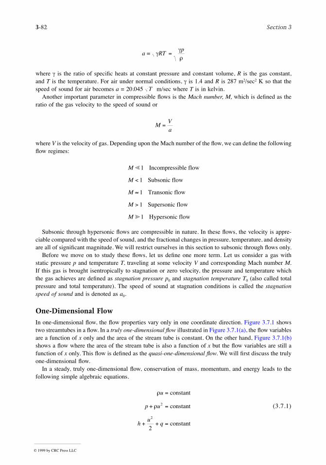
3-82 Section 3
where g is the ratio of speciÞc heats at constant pressure and constant volume, R is the gas constant,and T is the temperature. For air under normal conditions, g is 1.4 and R is 287 m2/sec2 K so that thespeed of sound for air becomes a = 20.045 m/sec where T is in kelvin.
Another important parameter in compressible ßows is the Mach number, M, which is deÞned as theratio of the gas velocity to the speed of sound or
where V is the velocity of gas. Depending upon the Mach number of the ßow, we can deÞne the followingßow regimes:
Subsonic through hypersonic ßows are compressible in nature. In these ßows, the velocity is appre-ciable compared with the speed of sound, and the fractional changes in pressure, temperature, and densityare all of signiÞcant magnitude. We will restrict ourselves in this section to subsonic through ßows only.
Before we move on to study these ßows, let us deÞne one more term. Let us consider a gas withstatic pressure p and temperature T, traveling at some velocity V and corresponding Mach number M.If this gas is brought isentropically to stagnation or zero velocity, the pressure and temperature whichthe gas achieves are deÞned as stagnation pressure p0 and stagnation temperature T0 (also called totalpressure and total temperature). The speed of sound at stagnation conditions is called the stagnationspeed of sound and is denoted as a0.
One-Dimensional Flow
In one-dimensional ßow, the ßow properties vary only in one coordinate direction. Figure 3.7.1 showstwo streamtubes in a ßow. In a truly one-dimensional ßow illustrated in Figure 3.7.1(a), the ßow variablesare a function of x only and the area of the stream tube is constant. On the other hand, Figure 3.7.1(b)shows a ßow where the area of the stream tube is also a function of x but the ßow variables are still afunction of x only. This ßow is deÞned as the quasi-one-dimensional ßow. We will Þrst discuss the trulyone-dimensional ßow.
In a steady, truly one-dimensional ßow, conservation of mass, momentum, and energy leads to thefollowing simple algebraic equations.
(3.7.1)
a RTp
= ggr
=
T
MV
a=
M
M
M
M
M
!
@
1
1
1
1
1
Incompressible flow
Subsonic flow
Transonic flow
Supersonic flow
Hypersonic flow
<
»
>
r
r
u
p u
hu
q
=
=
+ + =
constant
+ constant
constant
2
2
2
© 1999 by CRC Press LLC
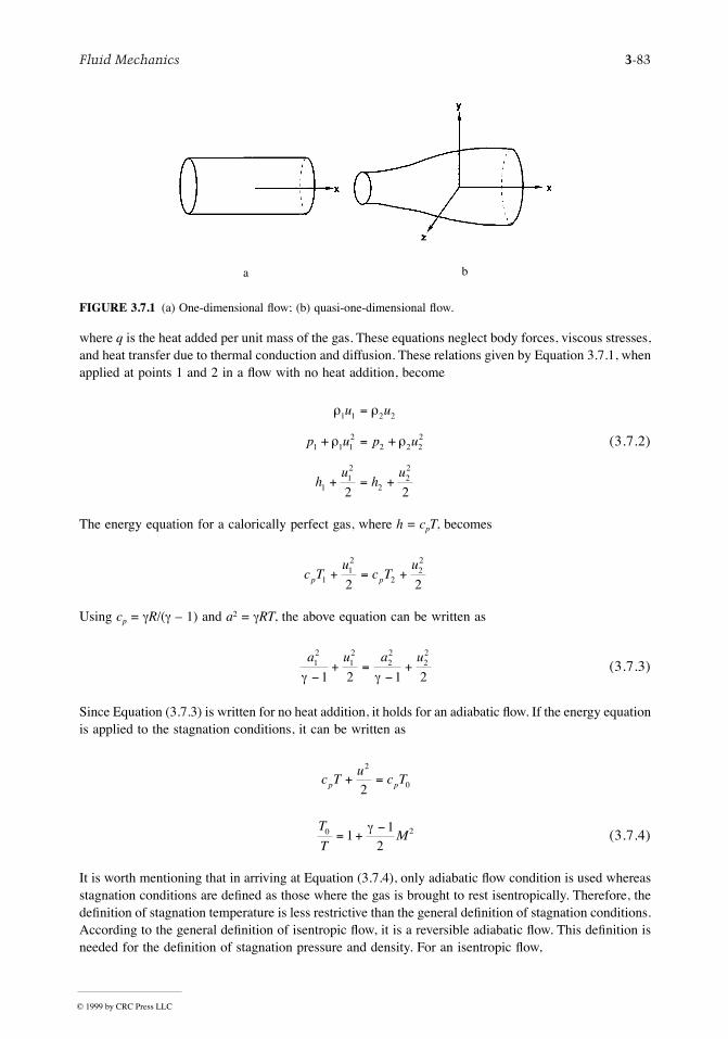
Fluid Mechanics 3-83
where q is the heat added per unit mass of the gas. These equations neglect body forces, viscous stresses,and heat transfer due to thermal conduction and diffusion. These relations given by Equation 3.7.1, whenapplied at points 1 and 2 in a ßow with no heat addition, become
(3.7.2)
The energy equation for a calorically perfect gas, where h = cpT, becomes
Using cp = gR/(g Ð 1) and a2 = gRT, the above equation can be written as
(3.7.3)
Since Equation (3.7.3) is written for no heat addition, it holds for an adiabatic ßow. If the energy equationis applied to the stagnation conditions, it can be written as
(3.7.4)
It is worth mentioning that in arriving at Equation (3.7.4), only adiabatic ßow condition is used whereasstagnation conditions are deÞned as those where the gas is brought to rest isentropically. Therefore, thedeÞnition of stagnation temperature is less restrictive than the general deÞnition of stagnation conditions.According to the general deÞnition of isentropic ßow, it is a reversible adiabatic ßow. This deÞnition isneeded for the deÞnition of stagnation pressure and density. For an isentropic ßow,
FIGURE 3.7.1 (a) One-dimensional ßow; (b) quasi-one-dimensional ßow.
a b
r r
r r
1 1 2 2
1 1 12
2 2 22
112
222
2 2
u u
p u p u
hu
hu
=
=
+ = +
+ +
c Tu
c Tu
p p112
222
2 2+ = +
a u a u12
12
22
22
1 2 1 2g g-+ =
-+
c Tu
c Tp p+ =2
02
T
TM0 21
12
= +-g
© 1999 by CRC Press LLC
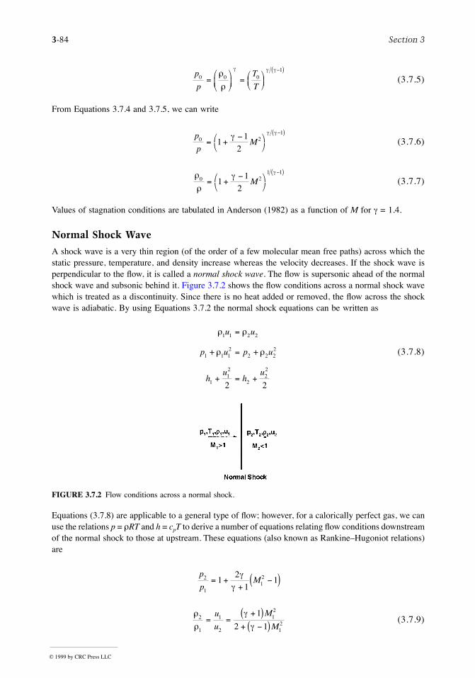
3-84 Section 3
(3.7.5)
From Equations 3.7.4 and 3.7.5, we can write
(3.7.6)
(3.7.7)
Values of stagnation conditions are tabulated in Anderson (1982) as a function of M for g = 1.4.
Normal Shock Wave
A shock wave is a very thin region (of the order of a few molecular mean free paths) across which thestatic pressure, temperature, and density increase whereas the velocity decreases. If the shock wave isperpendicular to the ßow, it is called a normal shock wave. The ßow is supersonic ahead of the normalshock wave and subsonic behind it. Figure 3.7.2 shows the ßow conditions across a normal shock wavewhich is treated as a discontinuity. Since there is no heat added or removed, the ßow across the shockwave is adiabatic. By using Equations 3.7.2 the normal shock equations can be written as
(3.7.8)
Equations (3.7.8) are applicable to a general type of ßow; however, for a calorically perfect gas, we canuse the relations p = rRT and h = cpT to derive a number of equations relating ßow conditions downstreamof the normal shock to those at upstream. These equations (also known as RankineÐHugoniot relations)are
(3.7.9)
FIGURE 3.7.2 Flow conditions across a normal shock.
p
p
T
T0 0 0
1
=æ
èç
ö
ø÷ = æ
èç
öø÷
-( )r
r
g g g
p
pM0 2
1
11
2= +
-æè
öø
-( )g g g
r
rg g
0 21 1
11
2= +
-æè
öø
-( )M
r r
r r
1 1 2 2
1 1 12
2 2 22
112
222
2 2
u u
p u p u
hu
hu
=
=
+ = +
+ +
p
pM2
1121
21
1= ++
-( )gg
r
r
g
g2
1
1
2
12
12
1
2 1= =
+( )+ -( )
u
u
M
M
© 1999 by CRC Press LLC
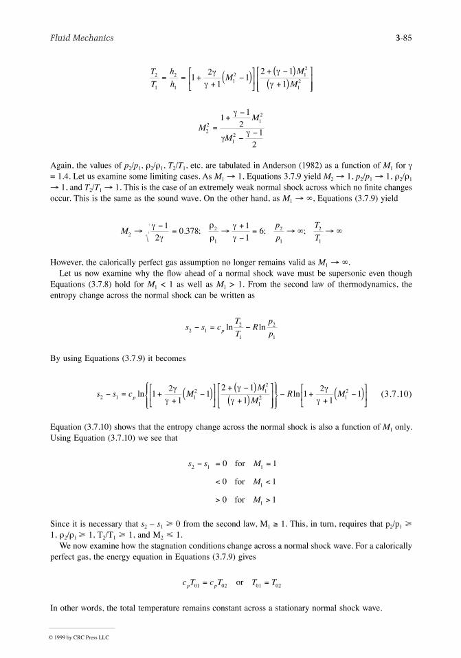
Fluid Mechanics 3-85
Again, the values of p2/p1, r2/r1, T2/T1, etc. are tabulated in Anderson (1982) as a function of M1 for g= 1.4. Let us examine some limiting cases. As M1 ® 1, Equations 3.7.9 yield M2 ® 1, p2/p1 ® 1, r2/r1
® 1, and T2/T1 ® 1. This is the case of an extremely weak normal shock across which no finite changesoccur. This is the same as the sound wave. On the other hand, as M1 ® ¥, Equations (3.7.9) yield
However, the calorically perfect gas assumption no longer remains valid as M1 ® ¥.Let us now examine why the ßow ahead of a normal shock wave must be supersonic even though
Equations (3.7.8) hold for M1 < 1 as well as M1 > 1. From the second law of thermodynamics, theentropy change across the normal shock can be written as
By using Equations (3.7.9) it becomes
(3.7.10)
Equation (3.7.10) shows that the entropy change across the normal shock is also a function of M1 only.Using Equation (3.7.10) we see that
Since it is necessary that s2 Ð s1 > 0 from the second law, M1 ³ 1. This, in turn, requires that p2/p1 >1, r2/r1 > 1, T2/T1 > 1, and M2 < 1.
We now examine how the stagnation conditions change across a normal shock wave. For a caloricallyperfect gas, the energy equation in Equations (3.7.9) gives
In other words, the total temperature remains constant across a stationary normal shock wave.
T
T
h
hM
M
M2
1
2
112 1
2
121
21
12 1
1= = +
+-( )é
ëê
ù
ûú
+ -( )+( )
é
ëêê
ù
ûúú
gg
g
g
MM
M22
12
12
11
21
2
=+
-
--
g
gg
Mp
p
T
T22
1
2
1
2
1
12
0 37811
6®-
= ®+-
= ® ¥ ® ¥g
g
r
rgg
. ; ; ;
s s cT
TR
p
pp2 12
1
2
1
- = -ln ln
s s c MM
MR Mp2 1 1
2 12
12 1
212
11
2 1
11
21
1- = ++
-( )é
ëê
ù
ûú
+ -( )+( )
é
ëêê
ù
ûúú
ìíï
îï
üýï
þï- +
+-( )é
ëê
ù
ûúln ln
gg
g
gg
g
s s M
M
M
2 1 1
1
1
0 1
0 1
0 1
- = =
< <
> >
for
for
for
c T c T T Tp p01 02 01 02= =or
© 1999 by CRC Press LLC
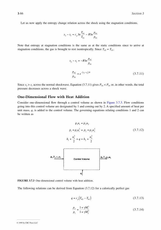
3-86 Section 3
Let us now apply the entropy change relation across the shock using the stagnation conditions.
Note that entropy at stagnation conditions is the same as at the static conditions since to arrive atstagnation conditions, the gas is brought to rest isentropically. Since T02 = T01,
(3.7.11)
Since s2 > s1 across the normal shockwave, Equation (3.7.11) gives P02 < P01 or, in other words, the totalpressure decreases across a shock wave.
One-Dimensional Flow with Heat Addition
Consider one-dimensional ßow through a control volume as shown in Figure 3.7.3. Flow conditionsgoing into this control volume are designated by 1 and coming out by 2. A speciÞed amount of heat perunit mass, q, is added to the control volume. The governing equations relating conditions 1 and 2 canbe written as
(3.7.12)
The following relations can be derived from Equation (3.7.12) for a calorically perfect gas
(3.7.13)
(3.7.14)
FIGURE 3.7.3 One-dimensional control volume with heat addition.
s s cT
TR
p
pp2 102
01
02
01
- = -ln ln
s s Rp
p2 102
01
- = - ln
p
pe
s s R02
01
2 1= - -( )
r r
r r
1 1 2 2
1 1 12
2 2 22
112
222
2 2
u u
p u p u
hu
q hu
=
=
+ + = +
+ +
q c T Tp= -( )02 01
p
p
M
M2
1
12
22
1
1=
+
+
g
g
© 1999 by CRC Press LLC
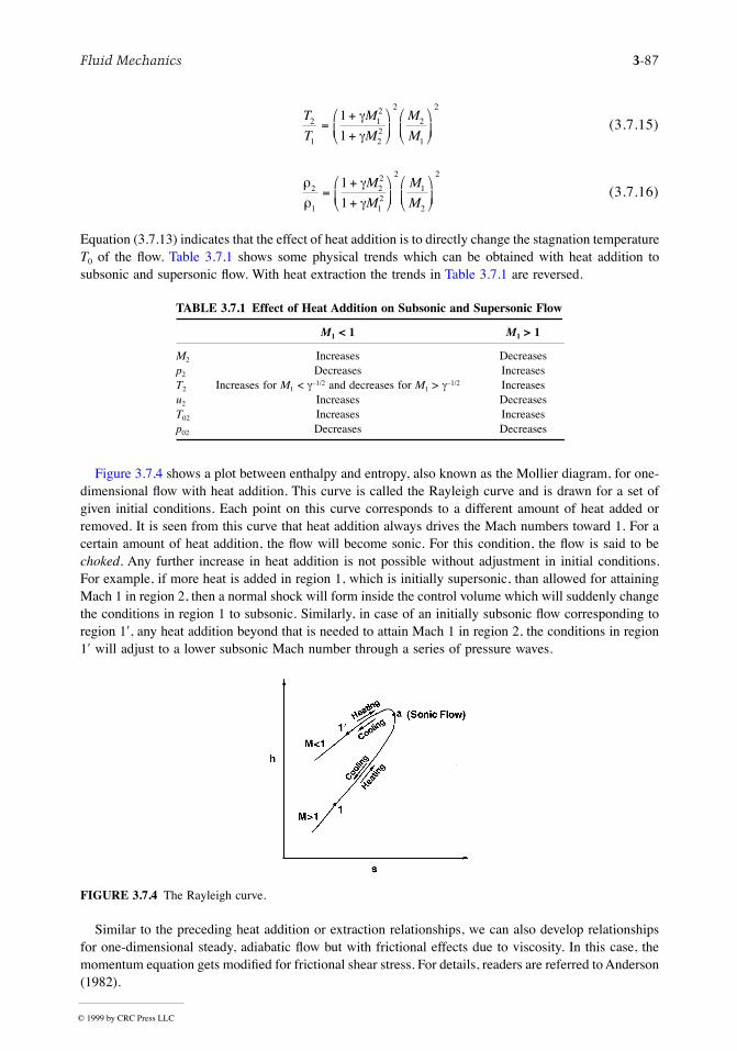
Fluid Mechanics 3-87
(3.7.15)
(3.7.16)
Equation (3.7.13) indicates that the effect of heat addition is to directly change the stagnation temperatureT0 of the ßow. Table 3.7.1 shows some physical trends which can be obtained with heat addition tosubsonic and supersonic ßow. With heat extraction the trends in Table 3.7.1 are reversed.
Figure 3.7.4 shows a plot between enthalpy and entropy, also known as the Mollier diagram, for one-dimensional ßow with heat addition. This curve is called the Rayleigh curve and is drawn for a set ofgiven initial conditions. Each point on this curve corresponds to a different amount of heat added orremoved. It is seen from this curve that heat addition always drives the Mach numbers toward 1. For acertain amount of heat addition, the ßow will become sonic. For this condition, the ßow is said to bechoked. Any further increase in heat addition is not possible without adjustment in initial conditions.For example, if more heat is added in region 1, which is initially supersonic, than allowed for attainingMach 1 in region 2, then a normal shock will form inside the control volume which will suddenly changethe conditions in region 1 to subsonic. Similarly, in case of an initially subsonic ßow corresponding toregion 1¢, any heat addition beyond that is needed to attain Mach 1 in region 2, the conditions in region1¢ will adjust to a lower subsonic Mach number through a series of pressure waves.
Similar to the preceding heat addition or extraction relationships, we can also develop relationshipsfor one-dimensional steady, adiabatic ßow but with frictional effects due to viscosity. In this case, themomentum equation gets modiÞed for frictional shear stress. For details, readers are referred to Anderson(1982).
TABLE 3.7.1 Effect of Heat Addition on Subsonic and Supersonic Flow
M1 < 1 M1 > 1
M2 Increases Decreasesp2 Decreases IncreasesT2 Increases for M1 < gÐ1/2 and decreases for M1 > gÐ1/2 Increasesu2 Increases DecreasesT02 Increases Increasesp02 Decreases Decreases
FIGURE 3.7.4 The Rayleigh curve.
T
T
M
M
M
M2
1
12
22
2
2
1
21
1=
+
+
æ
èç
ö
ø÷
æ
èç
ö
ø÷
g
g
r
r
g
g2
1
22
12
2
1
2
21
1=
+
+
æ
èç
ö
ø÷
æ
èç
ö
ø÷
M
M
M
M
© 1999 by CRC Press LLC
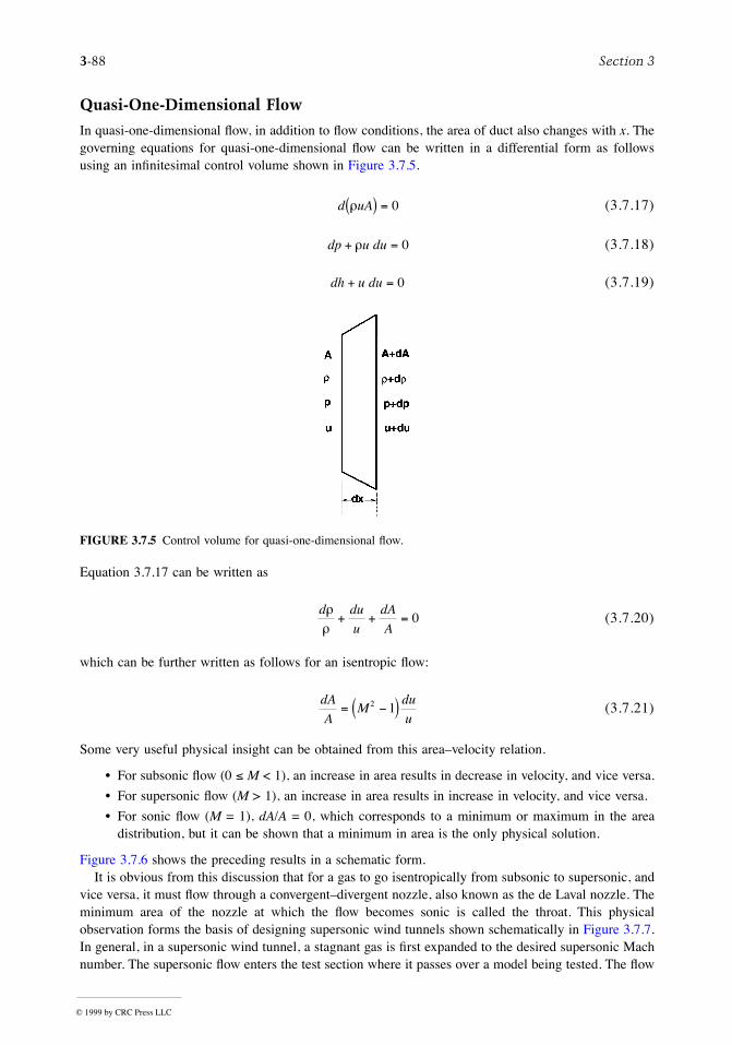
3-88 Section 3
Quasi-One-Dimensional Flow
In quasi-one-dimensional ßow, in addition to ßow conditions, the area of duct also changes with x. Thegoverning equations for quasi-one-dimensional ßow can be written in a differential form as followsusing an inÞnitesimal control volume shown in Figure 3.7.5.
(3.7.17)
(3.7.18)
(3.7.19)
Equation 3.7.17 can be written as
(3.7.20)
which can be further written as follows for an isentropic ßow:
(3.7.21)
Some very useful physical insight can be obtained from this areaÐvelocity relation.
¥ For subsonic ßow (0 £ M < 1), an increase in area results in decrease in velocity, and vice versa.
¥ For supersonic ßow (M > 1), an increase in area results in increase in velocity, and vice versa.
¥ For sonic ßow (M = 1), dA/A = 0, which corresponds to a minimum or maximum in the areadistribution, but it can be shown that a minimum in area is the only physical solution.
Figure 3.7.6 shows the preceding results in a schematic form.It is obvious from this discussion that for a gas to go isentropically from subsonic to supersonic, and
vice versa, it must ßow through a convergentÐdivergent nozzle, also known as the de Laval nozzle. Theminimum area of the nozzle at which the ßow becomes sonic is called the throat. This physicalobservation forms the basis of designing supersonic wind tunnels shown schematically in Figure 3.7.7.In general, in a supersonic wind tunnel, a stagnant gas is Þrst expanded to the desired supersonic Machnumber. The supersonic ßow enters the test section where it passes over a model being tested. The ßow
FIGURE 3.7.5 Control volume for quasi-one-dimensional ßow.
d uAr( ) = 0
dp u du+ =r 0
dh u du+ = 0
d du
u
dA
A
rr
+ + = 0
dA
AM
du
u= -( )2 1
© 1999 by CRC Press LLC
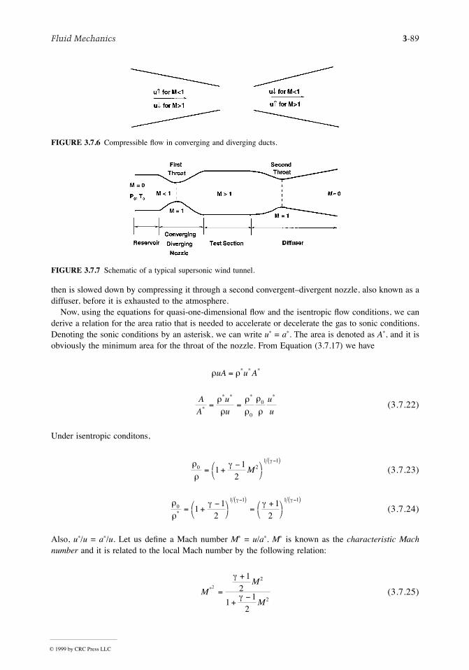
Fluid Mechanics 3-89
then is slowed down by compressing it through a second convergentÐdivergent nozzle, also known as adiffuser, before it is exhausted to the atmosphere.
Now, using the equations for quasi-one-dimensional ßow and the isentropic ßow conditions, we canderive a relation for the area ratio that is needed to accelerate or decelerate the gas to sonic conditions.Denoting the sonic conditions by an asterisk, we can write u* = a*. The area is denoted as A*, and it isobviously the minimum area for the throat of the nozzle. From Equation (3.7.17) we have
(3.7.22)
Under isentropic conditons,
(3.7.23)
(3.7.24)
Also, u*/u = a*/u. Let us deÞne a Mach number M* = u/a*. M* is known as the characteristic Machnumber and it is related to the local Mach number by the following relation:
(3.7.25)
FIGURE 3.7.6 Compressible ßow in converging and diverging ducts.
FIGURE 3.7.7 Schematic of a typical supersonic wind tunnel.
r ruA u A= * * *
A
A
u
u
u
u*
* * * *
= =rr
rr
r
r0
0
r
rg g
0 21 1
11
2= +
-æè
öø
-( )M
r
rg gg g
01 1 1 1
11
21
2* = +-æ
èöø
=+æ
èöø
-( ) -( )
MM
M
*2
12
11
2
2
2=
+
+-
g
g
© 1999 by CRC Press LLC
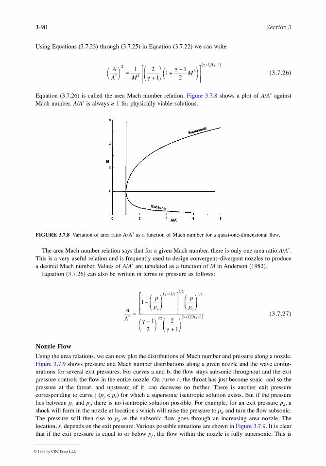
3-90 Section 3
Using Equations (3.7.23) through (3.7.25) in Equation (3.7.22) we can write
(3.7.26)
Equation (3.7.26) is called the area Mach number relation. Figure 3.7.8 shows a plot of A/A* againstMach number. A/A* is always ³ 1 for physically viable solutions.
The area Mach number relation says that for a given Mach number, there is only one area ratio A/A*.This is a very useful relation and is frequently used to design convergentÐdivergent nozzles to producea desired Mach number. Values of A/A* are tabulated as a function of M in Anderson (1982).
Equation (3.7.26) can also be written in terms of pressure as follows:
(3.7.27)
Nozzle Flow
Using the area relations, we can now plot the distributions of Mach number and pressure along a nozzle.Figure 3.7.9 shows pressure and Mach number distributions along a given nozzle and the wave conÞg-urations for several exit pressures. For curves a and b, the ßow stays subsonic throughout and the exitpressure controls the ßow in the entire nozzle. On curve c, the throat has just become sonic, and so thepressure at the throat, and upstream of it, can decrease no further. There is another exit pressurecorresponding to curve j (pj < pc) for which a supersonic isentropic solution exists. But if the pressurelies between pc and pj, there is no isentropic solution possible. For example, for an exit pressure pd, ashock will form in the nozzle at location s which will raise the pressure to pd¢ and turn the ßow subsonic.The pressure will then rise to pd as the subsonic ßow goes through an increasing area nozzle. Thelocation, s, depends on the exit pressure. Various possible situations are shown in Figure 3.7.9. It is clearthat if the exit pressure is equal to or below pf , the ßow within the nozzle is fully supersonic. This is
FIGURE 3.7.8 Variation of area ratio A/A* as a function of Mach number for a quasi-one-dimensional ßow.
A
A MM*
æè
öø
=+
æ
èç
ö
ø÷ +
-æè
öø
é
ëêê
ù
ûúú
+( ) -( )2
22
1 11 2
11
12g
gg g
A
A
p
p
p
p
* =
-æ
èç
ö
ø÷
é
ë
êê
ù
û
úú
æ
èç
ö
ø÷
-æè
öø +
æ
èç
ö
ø÷
-( )
+( ) -( )
1
12
21
0
11 2
0
1
1 2 1 2 1
g g g
g gg
g
© 1999 by CRC Press LLC
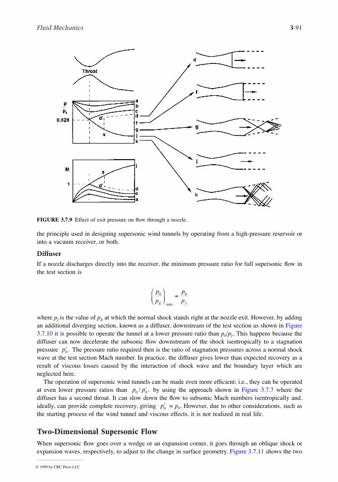
Fluid Mechanics 3-91
the principle used in designing supersonic wind tunnels by operating from a high-pressure reservoir orinto a vacuum receiver, or both.
Diffuser
If a nozzle discharges directly into the receiver, the minimum pressure ratio for full supersonic ßow inthe test section is
where pf is the value of pE at which the normal shock stands right at the nozzle exit. However, by addingan additional diverging section, known as a diffuser, downstream of the test section as shown in Figure3.7.10 it is possible to operate the tunnel at a lower pressure ratio than p0/pf . This happens because thediffuser can now decelerate the subsonic ßow downstream of the shock isentropically to a stagnationpressure The pressure ratio required then is the ratio of stagnation pressures across a normal shockwave at the test section Mach number. In practice, the diffuser gives lower than expected recovery as aresult of viscous losses caused by the interaction of shock wave and the boundary layer which areneglected here.
The operation of supersonic wind tunnels can be made even more efÞcient; i.e., they can be operatedat even lower pressure ratios than by using the approach shown in Figure 3.7.7 where thediffuser has a second throat. It can slow down the ßow to subsonic Mach numbers isentropically and,ideally, can provide complete recovery, giving = p0. However, due to other considerations, such asthe starting process of the wind tunnel and viscous effects, it is not realized in real life.
Two-Dimensional Supersonic Flow
When supersonic ßow goes over a wedge or an expansion corner, it goes through an oblique shock orexpansion waves, respectively, to adjust to the change in surface geometry. Figure 3.7.11 shows the two
FIGURE 3.7.9 Effect of exit pressure on ßow through a nozzle.
p
p
p
pE f
0 0æ
èç
ö
ø÷ =
min
¢p0 .
p p0 0/ ,¢
¢p0
© 1999 by CRC Press LLC
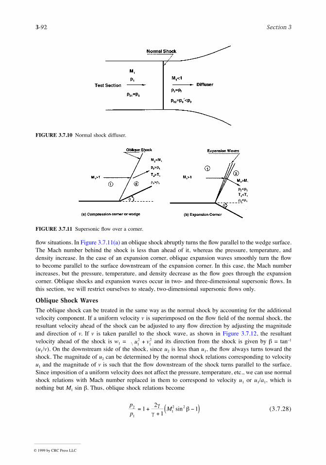
3-92 Section 3
ßow situations. In Figure 3.7.11(a) an oblique shock abruptly turns the ßow parallel to the wedge surface.The Mach number behind the shock is less than ahead of it, whereas the pressure, temperature, anddensity increase. In the case of an expansion corner, oblique expansion waves smoothly turn the ßowto become parallel to the surface downstream of the expansion corner. In this case, the Mach numberincreases, but the pressure, temperature, and density decrease as the ßow goes through the expansioncorner. Oblique shocks and expansion waves occur in two- and three-dimensional supersonic ßows. Inthis section, we will restrict ourselves to steady, two-dimensional supersonic ßows only.
Oblique Shock Waves
The oblique shock can be treated in the same way as the normal shock by accounting for the additionalvelocity component. If a uniform velocity v is superimposed on the ßow Þeld of the normal shock, theresultant velocity ahead of the shock can be adjusted to any ßow direction by adjusting the magnitudeand direction of v. If v is taken parallel to the shock wave, as shown in Figure 3.7.12, the resultantvelocity ahead of the shock is w1 = and its direction from the shock is given by b = tanÐ1
(u1/v). On the downstream side of the shock, since u2 is less than u1, the ßow always turns toward theshock. The magnitude of u2 can be determined by the normal shock relations corresponding to velocityu1 and the magnitude of v is such that the ßow downstream of the shock turns parallel to the surface.Since imposition of a uniform velocity does not affect the pressure, temperature, etc., we can use normalshock relations with Mach number replaced in them to correspond to velocity u1 or u1/a1, which isnothing but M1 sin b. Thus, oblique shock relations become
(3.7.28)
FIGURE 3.7.10 Normal shock diffuser.
FIGURE 3.7.11 Supersonic ßow over a corner.
u v12
12+
p
pM2
112 21
21
1= ++
-( )gg
bsin
© 1999 by CRC Press LLC
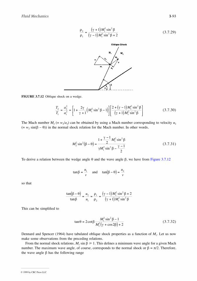
Fluid Mechanics 3-93
(3.7.29)
(3.7.30)
The Mach number M2 (= w2/a2) can be obtained by using a Mach number corresponding to velocity u2
(= w2 sin(b Ð q)) in the normal shock relation for the Mach number. In other words,
(3.7.31)
To derive a relation between the wedge angle q and the wave angle b, we have from Figure 3.7.12
so that
This can be simpliÞed to
(3.7.32)
Dennard and Spencer (1964) have tabulated oblique shock properties as a function of M1. Let us nowmake some observations from the preceding relations.
From the normal shock relations, M1 sin b > 1. This deÞnes a minimum wave angle for a given Machnumber. The maximum wave angle, of course, corresponds to the normal shock or b = p/2. Therefore,the wave angle b has the following range
FIGURE 3.7.12 Oblique shock on a wedge.
r
r
g b
g b2
1
12 2
12 2
1
1 2=
+( )-( ) +
M
M
sin
sin
T
T
a
aM
M
M2
1
22
12 1
2 2 12 2
12 21
21
12 1
1= = +
+-( )é
ëê
ù
ûú
+ -( )+( )
é
ëêê
ù
ûúú
gg
bg b
g bsin
sin
sin
MM
M22 2
12 2
12 2
11
21
2
sinsin
sinb q
gb
g bg-( ) =
+-
--
tanb b q= -( ) =u
v
u
v1 2and tan
tan b q
b
r
r
g b
g b
-( )= = =
-( ) +
+( )tan
sin
sin
u
u
M
M2
1
1
2
12 2
12 2
1 2
1
tan cotsin
cosq b
b
g b=
-
+( ) +2
1
2 212 2
12
M
M
© 1999 by CRC Press LLC
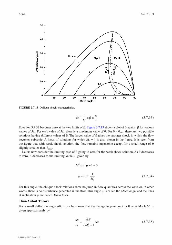
3-94 Section 3
(3.7.33)
Equation 3.7.32 becomes zero at the two limits of b. Figure 3.7.13 shows a plot of q against b for variousvalues of M1. For each value of M1, there is a maximum value of q. For q < qmax, there are two possiblesolutions having different values of b. The larger value of b gives the stronger shock in which the ßowbecomes subsonic. A locus of solutions for which M2 = 1 is also shown in the Þgure. It is seen fromthe Þgure that with weak shock solution, the ßow remains supersonic except for a small range of qslightly smaller than qmax.
Let us now consider the limiting case of q going to zero for the weak shock solution. As q decreasesto zero, b decreases to the limiting value m, given by
(3.7.34)
For this angle, the oblique shock relations show no jump in ßow quantities across the wave or, in otherwords, there is no disturbance generated in the ßow. This angle m is called the Mach angle and the linesat inclination m are called Mach lines.
Thin-Airfoil Theory
For a small deßection angle Dq, it can be shown that the change in pressure in a ßow at Mach M1 isgiven approximately by
(3.7.35)
FIGURE 3.7.13 Oblique shock characteristics.
sin- £ £1 12M
bp
M12 2 1 0sin m - =
m = -sin 1
1
1M
DD
p
p
M
M1
12
12 1
»-
gq
© 1999 by CRC Press LLC
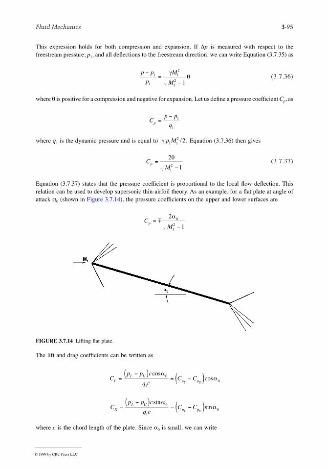
Fluid Mechanics 3-95
This expression holds for both compression and expansion. If Dp is measured with respect to thefreestream pressure, p1, and all deßections to the freestream direction, we can write Equation (3.7.35) as
(3.7.36)
where q is positive for a compression and negative for expansion. Let us deÞne a pressure coefÞcient Cp, as
where q1 is the dynamic pressure and is equal to Equation (3.7.36) then gives
(3.7.37)
Equation (3.7.37) states that the pressure coefÞcient is proportional to the local ßow deßection. Thisrelation can be used to develop supersonic thin-airfoil theory. As an example, for a ßat plate at angle ofattack a0 (shown in Figure 3.7.14), the pressure coefÞcients on the upper and lower surfaces are
The lift and drag coefÞcients can be written as
where c is the chord length of the plate. Since a0 is small, we can write
FIGURE 3.7.14 Lifting ßat plate.
p p
p
M
M
-=
-1
1
12
12 1
gq
Cp p
qp =- 1
1
g p M1 12 2/ .
CM
p =-
2
112
q
CM
p =-
m2
10
12
a
Cp p c
q cC CL
L Up pL U
=-( )
= -( )coscos
aa0
10
Cp p c
q cC CD
L Up pL U
=-( )
= -( )sinsin
aa0
10
© 1999 by CRC Press LLC
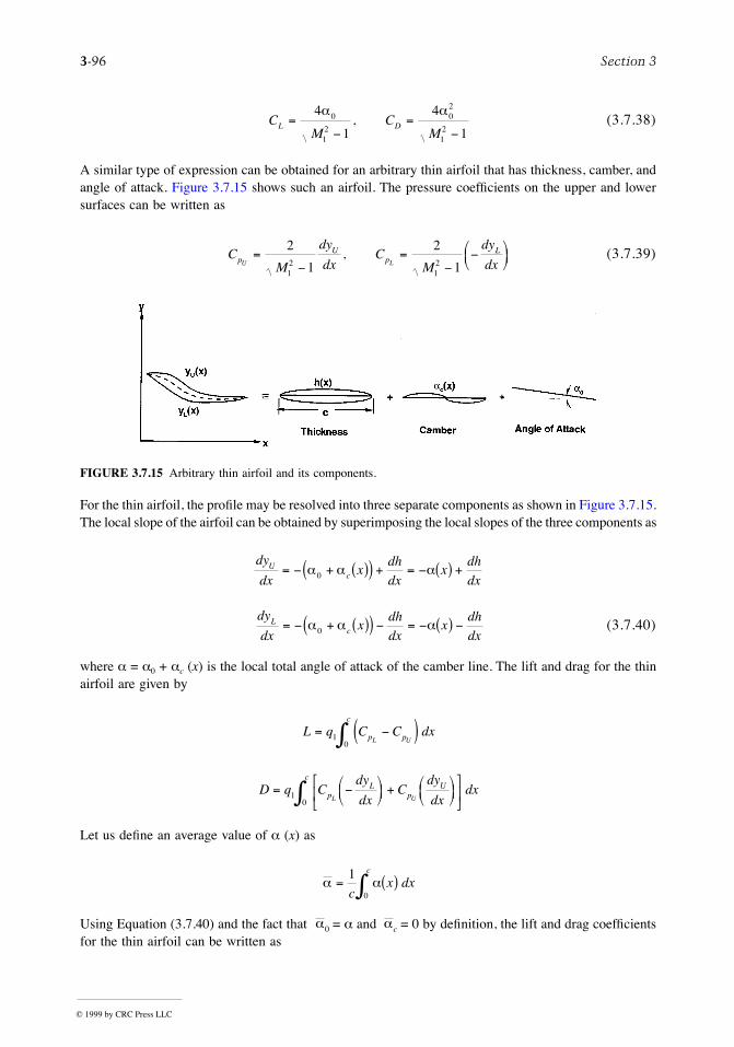
3-96 Section 3
(3.7.38)
A similar type of expression can be obtained for an arbitrary thin airfoil that has thickness, camber, andangle of attack. Figure 3.7.15 shows such an airfoil. The pressure coefÞcients on the upper and lowersurfaces can be written as
(3.7.39)
For the thin airfoil, the proÞle may be resolved into three separate components as shown in Figure 3.7.15.The local slope of the airfoil can be obtained by superimposing the local slopes of the three components as
(3.7.40)
where a = a0 + ac (x) is the local total angle of attack of the camber line. The lift and drag for the thinairfoil are given by
Let us deÞne an average value of a (x) as
Using Equation (3.7.40) and the fact that = a and = 0 by deÞnition, the lift and drag coefÞcientsfor the thin airfoil can be written as
FIGURE 3.7.15 Arbitrary thin airfoil and its components.
CM
CM
L D=-
=-
4
1
4
10
12
02
12
a a,
CM
dy
dxC
M
dy
dxpU
pL
U L=
-=
--æ
èç
öø÷
2
1
2
112
12
,
dy
dxx
dh
dxx
dh
dxU
c= - + ( )( ) + = - ( ) +a a a0
dy
dxx
dh
dxx
dh
dxL
c= - + ( )( ) - = - ( ) -a a a0
L q C C dxc
p pL U= -( )ò1
0
D q Cdy
dxC
dy
dxdx
c
pL
pU
L U= -æ
èç
öø÷ + æ
èç
öø÷
é
ëê
ù
ûúò1
0
a a= ( )ò1
0cx dx
c
a0 ac
© 1999 by CRC Press LLC
Fluid Mechanics 3-97
(3.7.41)
Equations (3.7.41) show that the lift coefÞcient depends only on the mean angle of attack whereas thedrag coefÞcient is a linear combination of the drag due to thickness, drag due to camber, and drag dueto lift (or mean angle of attack).
References
Anderson, J.D. 1982. Modern Compressible Flow, McGraw-Hill, New York.Dennard, J.S. and Spencer, P.B. 1964. Ideal-Gas Tables for Oblique-Shock Flow Parameters in Air at
Mach Numbers from 1.05 to 12.0. NASA TN D-2221.Liepmann, H.W. and Roshko, A. 1966. Elements of Gas Dynamics, John Wiley & Sons, New York.
Further Information
As mentioned in the beginning, this section discussed only one- or two-dimensional steady, inviscidcompressible ßows under perfect gas assumption. Even this discussion was quite brief because of spacelimitations. For more details on the subject as well as for compressible unsteady viscous ßows, readersare referred to Anderson (1982) and Liepmann and Roshko (1966).
CM
L =-
4
10
12
a
CM
dh
dxxD C=
-
æè
öø
+ ( ) +é
ëêê
ù
ûúú
4
112
22
02a a
© 1999 by CRC Press LLC
3-98 Section 3
3.8 Multiphase Flow
John C. Chen
Introduction
Classic study of ßuid mechanics concentrates on the ßow of a single homogeneous phase, e.g., water,air, steam. However, many industrially important processes involve simultaneous ßow of multiple phases,e.g., gas bubbles in oil, wet steam, dispersed particles in gas or liquid. Examples include vaporÐliquidßow in refrigeration systems, steamÐwater ßows in boilers and condensers, vaporÐliquid ßows indistillation columns, and pneumatic transport of solid particulates. In spite of their importance, multiphaseßows are often neglected in standard textbooks. Fundamental understanding and engineering designprocedures for multiphase ßows are not nearly so well developed as those for single-phase ßows. Anadded complexity is the need to predict the relative concentrations of the different phases in themultiphase ßows, a need that doesnÕt exist for single-phase ßows.
Inadequate understanding not withstanding, a signiÞcant amount of data have been collected andcombinations of theoretical models and empirical correlations are used in engineering calculations. Thisknowledge base is brießy summarized in this section and references are provided for additional infor-mation. While discussions are provided of solidÐgas ßows and solidÐliquid ßows, primary emphasis isplaced on multiphase ßow of gasÐliquids since this is the most often encountered class of multiphaseßows in industrial applications.
A multiphase ßow occurs whenever two or more of the following phases occur simultaneously:gas/vapor, solids, single-liquid phase, multiple (immiscible) liquid phases. Every possible combinationhas been encountered in some industrial process, the most common being the simultaneous ßow ofvapor/gas and liquid (as encountered in boilers and condensers). All multiphase ßow problems havefeatures which are characteristically different from those found in single-phase problems. First, therelative concentration of different phases is usually a dependent parameter of great importance inmultiphase ßows, while it is a parameter of no consequence in single-phase ßows. Second, the spatialdistribution of the various phases in the ßow channel strongly affects the ßow behavior, again a parameterthat is of no concern in single-phase ßows. Finally, since the density of various phases can differ byorders of magnitude, the inßuence of gravitational body force on multiphase ßows is of much greaterimportance than in the case of single-phase ßows. In any given ßow situation, the possibility exists forthe various phases to assume different velocities, leading to the phenomena of slip between phases andconsequent interfacial momentum transfer. Of course, the complexity of laminar/turbulent characteristicsoccurs in multiphase ßows as in single-phase ßows, with the added complexity of interactions betweenphases altering the laminar/turbulent ßow structures. These complexities increase exponentially with thenumber of phases encountered in the multiphase problem. Fortunately, a large number of applicationsoccur with just two phase ßows, or can be treated as pseudo-two-phase ßows.
Two types of analysis are used to deal with two-phase ßows. The simpler approach utilizes homoge-neous models which assume that the separate phases ßow with the same identical local velocity at allpoints in the ßuid. The second approach recognizes the possibility that the two phases can ßow atdifferent velocities throughout the ßuid, thereby requiring separate conservation equations for mass andmomentum for each phase. Brief descriptions of both classes of models are given below.
Fundamentals
Consider n phases in concurrent ßow through a duct with cross-sectional area Ac. Fundamental quantitiesthat characterize this ßow are
© 1999 by CRC Press LLC
Fluid Mechanics 3-99
Basic relationships between these and related parameters are
(3.8.1)
(3.8.2)
(3.8.3)
(3.8.4)
(3.8.5)
In most engineering calculations, the above parameters are deÞned as average quantities across the entireßow area, Ac. It should be noted, however, that details of the multiphase ßow could involve local variationsacross the ßow area. In the latter situation, Gi, vi, and ai are often deÞned on a local basis, varying withtransverse position across the ßow area.
Pressure drop along the ßow channel is associated with gravitational body force, acceleration forces,and frictional shear at the channel wall. The total pressure gradient along the ßow axis can be representedas
(3.8.6)
Çm i
u i
i
i
i
i
=
=
=
mass flow rate of th phase
velocity of th phase
volume fraction of th phase in channela
G i
m
A
i
i
c
=
=
mass flux of th phase
Ç
v i
G
i
i
i
=
=
superficial velocity of th phase
r
u i
v
i
i
i
=
=
actual velocity of th phase
a
x i
m
m
G
G
i
i
i
i
ni
i
i
n
=
= =
å å=
flow quality of th phase
Ç
1
a
r
r
i
i
i i
i
i ii
n
i
x
u
x
u
=
=
æ
èç
ö
ø÷
æ
èç
ö
ø÷
=å
volume fraction of th phase
1
dP
dz
dP
dz
dP
dz
dP
dzg a f
= æè
öø
+ æè
öø
+ æè
öø
© 1999 by CRC Press LLC
3-100 Section 3
where
(3.8.7)
and
(3.8.10)
(3.8.11)
In applications, the usual requirement is to determine pressure gradient (dP/dz) and the volumefractions (ai). The latter quantities are of particular importance since the volume fraction of individualphases affects all three components of the pressure gradient, as indicated in Equations (3.8.7) to (3.8.11).Correlations of various types have been developed for prediction of the volume fractions, all but thesimplest of which utilize empirical parameters and functions.
The simplest ßow model is known as the homogeneous equilibrium model (HEM), wherein all phasesare assumed to be in neutral equilibrium. One consequence of this assumption is that individual phasevelocities are equal for all phases everywhere in the ßow system:
(3.8.12)
This assumption permits direct calculation of the volume fractions from known mass qualities:
(3.8.13)
The uniform velocity for all phases is the same as mixture velocity:
(3.8.8)
(3.8.9)
dP
dzg
gi i
i
næè
öø
= - ×=
åcosq a r1
q = angle of channel from vertical
dP
dzG
du
dzai
i
n
iæè
öø
= -=
å1
dP
dz
u
Df
f
æè
öø
= -r 2
2
r
r a
=
==
å
density of multiphase mixture
i i
i
n
1
u
Gi
i
n
=
==
å
an average mixture velocity
1
1r
f = equivalent Darcy friction factor for the multiphase flow
u u ii = for all
a
rr
ii
ii
ii
n
x
x=
æ
èç
ö
ø÷
=å
1
© 1999 by CRC Press LLC
Fluid Mechanics 3-101
(3.8.14)
where
(3.8.15)
This homogeneous model permits direct evaluation of all three components of axial pressure gradient,if ßow qualities (xi) are known:
(3.8.16)
(3.8.17)
(3.8.18)
where u and r are given by Equations (3.8.14) and (3.8.15).Predicting the coefÞcient of friction (f to clear) remains a problem, even in the homogeneous model.
For cases of fully turbulent ßows, experience has shown that a value of 0.02 may be used as a Þrst-order approximation for (f to clear). More-accurate estimates require empirical correlations, speciÞc toparticular classes of multiphase ßows and subcategories of ßow regimes.
The following parts of this section consider the more common situations of two-phase ßows anddescribe improved design methodologies speciÞc to individual situations.
Gas–Liquid Two-Phase Flow
The most common case of multiphase ßow is two-phase ßow of gas and liquid, as encountered in steamgenerators and refrigeration systems. A great deal has been learned about such ßows, including delin-eation of ßow patterns in different ßow regimes, methods for estimating volume fractions (gas voidfractions), and two-phase pressure drops.
Flow Regimes
A special feature of multiphase ßows is their ability to assume different spatial distributions of thephases. These different ßow patterns have been classiÞed in ßow regimes, which are themselves alteredby the direction of ßow relative to gravitational acceleration. Figures 3.8.1 and 3.8.2 (Delhaye, 1981)show the ßow patterns commonly observed for co-current ßow of gas and liquid in vertical and horizontalchannels, respectively. For a constant liquid ßow rate, the gas phase tends to be distributed as smallbubbles at low gas ßow rates. Increasing gas ßow rate causes agglomeration of bubbles into larger slugsand plugs. Further increasing gas ßow rate causes separation of the phases into annular patterns whereinliquid concentrates at the channel wall and gas ßows in the central core for vertical ducts. For horizontalducts, gravitational force tends to drain the liquid annulus toward the bottom of the channel, resulting
u Gi
i
n
==
å1
1r
1
1r r
=æ
èç
ö
ø÷
=å xi
ii
n
dP
dz
g
xg i
ii
næè
öø
= -æ
èç
ö
ø÷
=å
cosq
r1
dP
dzG
du
dzai
i
næè
öø
= -æ
èç
ö
ø÷ ×
=å
1
dP
dz
u
Df
f f
æè
öø
= - ×r 2
2
© 1999 by CRC Press LLC
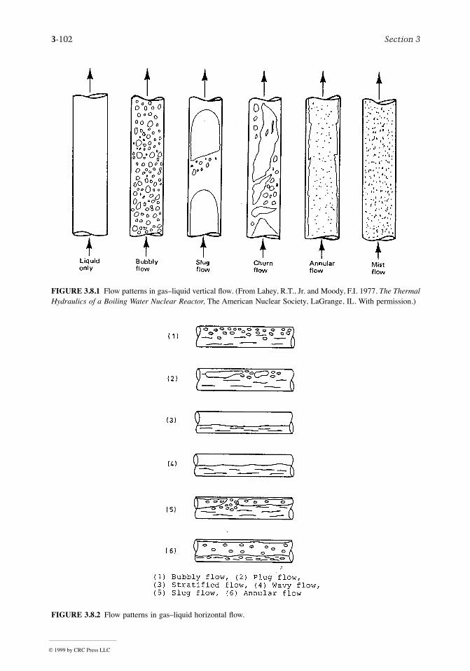
3-102 Section 3
FIGURE 3.8.1 Flow patterns in gasÐliquid vertical ßow. (From Lahey, R.T., Jr. and Moody, F.I. 1977. The ThermalHydraulics of a Boiling Water Nuclear Reactor, The American Nuclear Society, LaGrange, IL. With permission.)
FIGURE 3.8.2 Flow patterns in gasÐliquid horizontal ßow.
© 1999 by CRC Press LLC
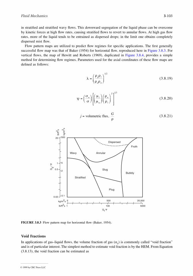
Fluid Mechanics 3-103
in stratiÞed and stratiÞed wavy ßows. This downward segregation of the liquid phase can be overcomeby kinetic forces at high ßow rates, causing stratiÞed ßows to revert to annular ßows. At high gas ßowrates, more of the liquid tends to be entrained as dispersed drops; in the limit one obtains completelydispersed mist ßow.
Flow pattern maps are utilized to predict ßow regimes for speciÞc applications. The Þrst generallysuccessful ßow map was that of Baker (1954) for horizontal ßow, reproduced here in Figure 3.8.3. Forvertical ßows, the map of Hewitt and Roberts (1969), duplicated in Figure 3.8.4, provides a simplemethod for determining ßow regimes. Parameters used for the axial coordinates of these ßow maps aredeÞned as follows:
(3.8.19)
(3.8.20)
(3.8.21)
Void Fractions
In applications of gasÐliquid ßows, the volume fraction of gas (ag) is commonly called Òvoid fractionÓand is of particular interest. The simplest method to estimate void fraction is by the HEM. From Equation(3.8.13), the void fraction can be estimated as
FIGURE 3.8.3 Flow pattern map for horizontal ßow (Baker, 1954).
lr r
r r=
æ
èç
ö
ø÷
g
a w
l
1 2
ys
s
m
m
r
r= æ
èç
öø÷
æ
èç
ö
ø÷
æ
èç
ö
ø÷
é
ë
êê
ù
û
úú
w
w
wl
l
2 1 3
jG
= volumetric flux, r
Dispersed
Annular
Slug
Plug
Bubbly
Froth
Wavy
Stratified
1 5000
20,0005 500
100
Gf Y
kg/m2s
lb/ft2s
50020
1
0.5
0.02 0.1
5
2
lb/ft
2 s
kg/m
2 s
Gg
/ Y
© 1999 by CRC Press LLC
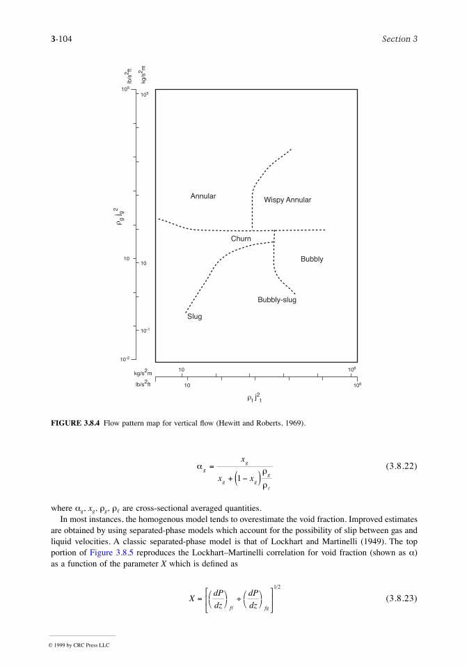
3-104 Section 3
(3.8.22)
where ag, xg, rg, r, are cross-sectional averaged quantities.In most instances, the homogenous model tends to overestimate the void fraction. Improved estimates
are obtained by using separated-phase models which account for the possibility of slip between gas andliquid velocities. A classic separated-phase model is that of Lockhart and Martinelli (1949). The topportion of Figure 3.8.5 reproduces the LockhartÐMartinelli correlation for void fraction (shown as a)as a function of the parameter X which is deÞned as
(3.8.23)
FIGURE 3.8.4 Flow pattern map for vertical ßow (Hewitt and Roberts, 1969).
105
rt j2t
Wispy Annular
Bubbly-slug
Slug
Churn
Annular
Bubbly
10-2
10
105
10-1
10
10 106
10610
r g j g2
kg/s2m
lb/s2ft
lb/s
2 ft
kg/s
2 m
a r
r
gg
g gg
x
x x=
+ -( )1l
XdP
dz
dP
dzf fg
= æè
öø
¸ æè
öø
é
ëê
ù
ûú
l
1 2
© 1999 by CRC Press LLC
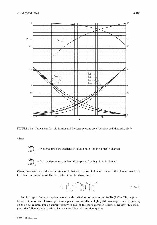
Fluid Mechanics 3-105
where
Often, ßow rates are sufÞciently high such that each phase if ßowing alone in the channel would beturbulent. In this situation the parameter X can be shown to be
(3.8.24)
Another type of separated-phase model is the drift-ßux formulation of Wallis (1969). This approachfocuses attention on relative slip between phases and results in slightly different expressions dependingon the ßow regime. For co-current upßow in two of the more common regimes, the drift-ßux modelgives the following relationships between void fraction and ßow quality:
FIGURE 3.8.5 Correlations for void fraction and frictional pressure drop (Lockhart and Martinelli, 1949)
10 10
100 10
0.1 10
1.0 10
(1 - a) a
f f
11
(1 - a)
a
101 1000.10.01X
ffttffvtfftvffvv
fgttfgtvfgvtfgvv
dP
dz f
æè
öø
=l
frictional pressure gradient of liquid phase flowing alone in channel
dP
dz fg
æè
öø
= frictional pressure gradient of gas phase flowing alone in channel
Xx
xttg
g
g
g
=-æ
èç
ö
ø÷
æ
èç
ö
ø÷
æ
èç
ö
ø÷
10 9 0 5 0 1. . .
r
r
m
ml
l
© 1999 by CRC Press LLC
3-106 Section 3
Bubbly ßow or churn-turbulent ßow:
(3.8.25)
Dispersed drop (mist) ßow:
(3.8.26)
where uo = terminal rise velocity of bubble, in bubbly ßow, or terminal fall velocity of drop in churn-turbulent ßow
Co = an empirical distribution coefÞcient . 1.2
Pressure Drop
Equations 3.8.16 through 3.8.18 permit calculation of two-phase pressure drop by the homogeneousmodel, if the friction coefÞcient (f) is known. One useful method for estimating (f) is to treat the entiretwo-phase ßow as if it were all liquid, except ßowing at the two-phase mixture velocity. By this approachthe frictional component of the two-phase pressure drop becomes
(3.8.27)
where (dP/dz)f,G = frictional pressure gradient if entire ßow (of total mass ßux G) ßowed as liquid inthe channel.
The equivalent frictional pressure drop for the entire ßow as liquid, (dP/dz)f,g, can be calculated bystandard procedures for single-phase ßow. In using Equations (3.8.16) through (3.8.18), the void fractionwould be calculated with the equivalent homogeneous expression Equation (3.8.13).
A more accurate method to calculate two-phase pressure drop is by the separated-phases model ofLockhart and Martinelli (1949). The bottom half of Figure 3.8.5 shows empirical curves for the Lock-hartÐMartinelli frictional multiplier, f:
(3.8.28)
where (i) denotes either the ßuid liquid phase (f) or gas phase (g). The single-phase frictional gradientis based on the ith phase ßowing alone in the channel, in either viscous laminar (v) or turbulent (t)modes. The most common case is where each phase ßowing alone would be turbulent, whence one coulduse Figure 3.8.5 to obtain
ar r
r
gg
o go g g
g
x
u
GC x x
=æ
èç
ö
ø÷ + + -( )é
ëê
ù
ûú1
l
x
u
Gg
go
g
gg
=- -( ) +æ
èç
öø÷
- -( ) -æ
èç
ö
ø÷
1 1 1
1 1 1
2ar
a
ar
r
l
l
dP
dzx
dP
dzfg
g f G
æè
öø
= + -æ
èç
ö
ø÷
é
ëêê
ù
ûúú
× æè
öø
1 1r
rl
l
fif fi
dP
dz
dP
dz= æ
èöø
¸ æè
öø
é
ëê
ù
ûú
1 2
© 1999 by CRC Press LLC
Fluid Mechanics 3-107
(3.8.29)
where (dP/dz)fg is calculated for gas phase ßowing alone and X = Xtt as given by Equation (3.8.24).The correlation of LockhartÐMartinelli has been found to be adequate for two-phase ßows at low-to-
moderate pressures, i.e., with reduced pressures less than 0.3. For applications at higher pressures, therevised models of Martinelli and Nelson (1948) and Thom (1964) are recommended.
Gas–Solid, Liquid–Solid Two-Phase Flows
Two-phase ßows can occur with solid particles in gas or liquid. Such ßows are found in handling ofgranular materials and heterogeneous reaction processing. Concurrent ßow of solid particulates with aßuid phase can occur with various ßow patterns, as summarized below.
Flow Regimes
Consider vertical upßow of a ßuid (gas or liquid) with solid particles. Figure 3.8.6 illustrates the majorßow regimes that have been identiÞed for such two-phase ßows. At low ßow rates, the ßuid phasepercolates between stationary particles; this is termed ßow through a Þxed bed. At some higher velocitya point is reached when the particles are all suspended by the upward ßowing ßuid, the drag forcebetween particles and ßuid counterbalancing the gravitational force on the particles. This is the point ofminimum ßuidization, marking the transition from Þxed to ßuidized beds. Increase of ßuid ßow ratebeyond minimum ßuidization causes instabilities in the two-phase mixture, and macroscopic bubbles orchannels of ßuid are observed in the case of gaseous ßuids. In the case of liquid ßuids, the two-phasemixture tends to expand, often without discrete bubbles or channels. Further increase of ßuid velocitycauses transition to turbulent ßuidization wherein discrete regions of separated phases (ßuid slugs orchannels and disperse suspensions of particles) can coexist. Depending on speciÞc operating conditions(e.g., superÞcial ßuid velocity, particle size, particle density, etc.), net transport of solid particles withthe ßowing ßuid can occur at any velocity equal to or greater than that associated with slug ßow andturbulent ßow. Further increases in ßuid velocity increase the net transport of solid particles. This canoccur with large-scale clusters of solid particles (as exempliÞed by the fast ßuidization regime) or withdilute dispersions of solid particles (as often utilized in pneumatic conveying). For engineering applica-tion of ßuidÐsolid two-phase ßows, the important thresholds between ßow regimes are marked by theßuid velocity for minimum ßuidization, terminal slip, and saltation threshold.
Minimum Fluidization
The transition from ßow through packed beds to the ßuidization regime is marked by the minimumßuidization velocity of the ßuid. On a plot pressure drop vs. superÞcial ßuid velocity, the point ofminimum ßuidization is marked by a transition from a linearly increasing pressure drop to a relativelyconstant pressure drop as shown in Figure 3.8.7 for typical data, for two-phase ßow of gas with sandparticles of 280 mm mean diameter (Chen, 1996). The threshold ßuid velocity at minimum ßuidizationis traditionally derived from the CarmanÐKozeny equation,
(3.8.30)
dP
dz
dP
dz
f
gttfg
æè
öø
=
= × æè
öø
frictional pressure gradient for two-phase flow
f2
Udp g
mf
s f
f
mf
mf
=-( )( )
×-( )
r r f
m
a
a
2 2
150 1
© 1999 by CRC Press LLC
3-108 Section 3
where f = sphericity of particles (unity for spherical particles)
amf = volumetric fraction of ßuid at minimum ßuidization
Small, light particles have minimum ßuidization voidage (amf) of the order 0.6, while larger particlessuch as sand have values closer to 0.4.
FIGURE 3.8.6 Flow patterns for vertical upßow of solid particles and gas or liquid. (From Chen, J.C. 1994. Proc.Xth Int. Heat Transfer Conf., Brighton, U.K., 1:369Ð386. With permission.)
FIGURE 3.8.7 Transition at minimum ßuidization. (From Chen, J.C. 1996. In Annual Review of Heat Transfer,Vol. VII, Begal House, Washington, D.C. With permission.)
© 1999 by CRC Press LLC
Fluid Mechanics 3-109
An alternative correlation for estimating the point of minimum ßuidization is that of Wen and Yu(1966):
(3.8.31)
where When the ßuid velocity exceeds Umf , the two-phase mixture exists in the ßuidized state in which the
pressure gradient is essentially balanced by the gravitational force on the two-phase mixture:
(3.8.32)
This ßuidized state exists until the ßuid velocity reaches a signiÞcant fraction of the terminal slip velocity,beyond which signiÞcant entrainment and transport of the solid particles occur.
Terminal Slip Velocity
For an isolated single particle the maximum velocity relative to an upßowing ßuid is the terminal slipvelocity. At this condition, the interfacial drag of the ßuid on the particle exactly balances the gravitationalbody force on the particle:
(3.8.33)
where CD = coefÞcient of drag on the particle.The coefÞcient of drag on the particle (CD) depends on the particle Reynolds number:
(3.8.34)
The following expressions may be used to estimate CD as appropriate:
(3.8.35)
Pneumatic Conveying
A desirable mode of pneumatic conveying is two-phase ßow with solid particles dispersed in theconcurrent ßowing ßuid. Such dispersed ßows can be obtained if the ßuid velocity is sufÞciently high.For both horizontal and vertical ßows, there are minimum ßuid velocities below which saltation of thesolid particles due to gravitational force occurs, leading to settling of the solid particles in horizontalchannels and choking of the particles in vertical channels. Figures 3.8.8 and 3.8.9 for Zenz and Othmer(1960) show these different regimes of pneumatic conveying for horizontal and vertical transport,respectively. Figure 3.8.8 shows that for a given rate of solids ßow (W) there is a minimum superÞcialßuid velocity below which solid particles tend to settle into a dense layer at the bottom of the horizontalchannels. Above this saltation threshold, fully dispersed two-phase ßow is obtained. In the case of
U dGamf p f
f
r
m= +( ) -33 7 0 041 33 7
0 5. . .
.
Ga d gf p s f f= -r r r m3 2( ) / .
dP
dzg s s f f= +[ ]a r a r
U U Ud
Ct f s t
p s f
f D
= -( ) =-( )
×é
ë
êê
ù
û
úú
4
31
1 2
r r
r
Re p
f p f s
f
d U U=
-( )r
m
C
C
Dp
p
Dp
p
= £
= £ £
321
18 51 103
ReRe
ReRe0.67
,
.,
© 1999 by CRC Press LLC
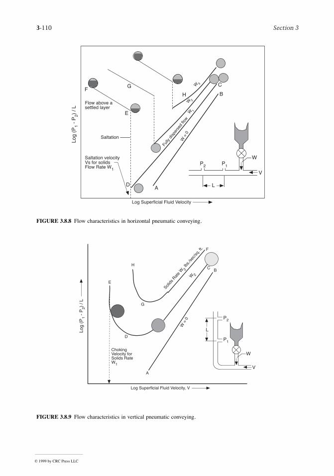
3-110 Section 3
FIGURE 3.8.8 Flow characteristics in horizontal pneumatic conveying.
FIGURE 3.8.9 Flow characteristics in vertical pneumatic conveying.
Log
(P1
- P
2) /
L
FG
E
H
AD
B
CW 3
W 2W 1
Fully
disp
erse
d flo
w
Flow above asettled layer
Saltation velocityVs for solidsFlow Rate W1
Saltation
W =
0L
V
P1P2
W
Log Superficial Fluid Velocity
Log Superficial Fluid Velocity, V
Log
(P1
- P
2) /
L
H
G
D
E
A
BC
F
Solids
Rat
e W 2
lbs./
sec/s
q. ft
.
W 2
W =
0
V
W
L
P2
P1
Choking Velocity for Solids Rate W1
© 1999 by CRC Press LLC
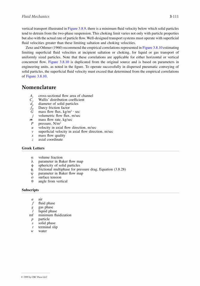
Fluid Mechanics 3-111
vertical transport illustrated in Figure 3.8.9, there is a minimum ßuid velocity below which solid particlestend to detrain from the two-phase suspension. This choking limit varies not only with particle propertiesbut also with the actual rate of particle ßow. Well-designed transport systems must operate with superÞcialßuid velocities greater than these limiting saltation and choking velocities.
Zenz and Othmer (1960) recommend the empirical correlations represented in Figure 3.8.10 estimatinglimiting superÞcial ßuid velocities at incipient saltation or choking, for liquid or gas transport ofuniformly sized particles. Note that these correlations are applicable for either horizontal or verticalconcurrent ßow. Figure 3.8.10 is duplicated from the original source and is based on parameters inengineering units, as noted in the Þgure. To operate successfully in dispersed pneumatic conveying ofsolid particles, the superÞcial ßuid velocity must exceed that determined from the empirical correlationsof Figure 3.8.10.
NomenclatureAc cross-sectional ßow area of channelCo WallisÕ distribution coefÞcientdp diameter of solid particlesfD Darcy friction factorG mass ßow ßux, kg/m2 á secj volumetric ßow ßux, m/sec
mass ßow rate, kg/secP pressure, N/m2
u velocity in axial ßow direction, m/secv superÞcial velocity in axial ßow direction, m/secx mass ßow qualityz axial coordinate
Greek Letters
a volume fractionl parameter in Baker ßow mapf sphericity of solid particlesfi frictional multiphase for pressure drag, Equation (3.8.28)y parameter in Baker ßow maps surface tensionq angle from vertical
Subscripts
a airf ßuid phaseg gas phasel liquid phase
mf minimum ßuidizationp particles solid phaset terminal slip
w water
Çm
© 1999 by CRC Press LLC
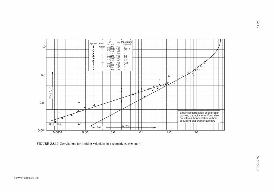
3-112Section
3
© 1999 by CRC Press LL
1.0 10
Empirical correlation of saturation carrying capacity for uniform size particles in horizontal or vertical cocurrent disperse phase flow
C
FIGURE 3.8.10 Correlations for limiting velocities in pneumatic conveying. (
1.0
0.1
0.01
0.0010.0001 0.001 0.01 0.1
Water******
Air***
0.00950.009820.01260.0230.02290.009850.06370.0660.03660.02310.0066
16216216216216516516568
165155131
310-12*15.55.55.51.75***
Symbol FluidDr
Inchesrp Pipe Diam.
(inches)
Liquid - SolidGas - Solid
W / Vrf
V2
/ g D
p r r2
Fluid Mechanics 3-113
References
Baker, O. 1954. Design of pipelines for simultaneous ßow of oil and gas, Oil Gas J..Chen, J.C. 1994. Two-phase ßow with and without phase changes: suspension ßows. Keynote lecture,
Proc. Xth Int. Heat Transfer Conf., Brighton, U.K., 1:369Ð386.Chen, J.C. 1996. Heat transfer to immersed surfaces in bubbling ßuidized beds, in Annual Review of
Heat Transfer, Vol. VII, Bengel House, Washington, D.C.Collier, J.G. 1972. Convective Boiling and Condensation, McGraw-Hill, London.Delhaye, J.M. 1981. Two-phase ßow patterns, in Two-Phase Flow and Heat Transfer, A.E. Bergles, J.G.
Collier, J.M. Delhaye, G.F. Newitt, and F. Mayinger, Eds., Hemisphere Publishing, McGraw-Hill,New York.
Hewitt, G.F. and Roberts, D.N. 1969. Studies of Two-Phase Flow Patterns by Simultaneous X-Ray andFlash Photography, Report AERE-M 2159.
Lahey, R.T., Jr. and Moody, F.I. 1977. The Thermal Hydraulics of a Boiling Water Nuclear Reactor, TheAmerican Nuclear Society, La Grange, IL.
Lockhart, R.W. and Martinelli, R.C. 1949. Proposed correlation of data for isothermal two-phase two-component ßow in pipes, Chem. Eng. Progr., 45:39.
Martinelli, R.C. and Nelson, D.B. 1984. Prediction of pressure drop during forced-circulation boilingof water, Trans. ASME, 70:695Ð702.
Thom, J.R.S. 1964. Prediction of pressure drop during forced circulation boiling of water, Int. J. HeatMass Transfer, 7:709Ð724.
Wallis, G.B. 1969. One-Dimensional Two-Phase Flow, McGraw-Hill, New York.Wen, C.Y. and Yu, Y.H. 1966. A generalized method of predicting the minimum ßuidization velocity,
AIChE J., 12:610Ð612.Zenz, F.A. and Othmer, D.F. 1960. Fluidization and Fluid-Particle Systems, Reinhold, New York.
© 1999 by CRC Press LLC
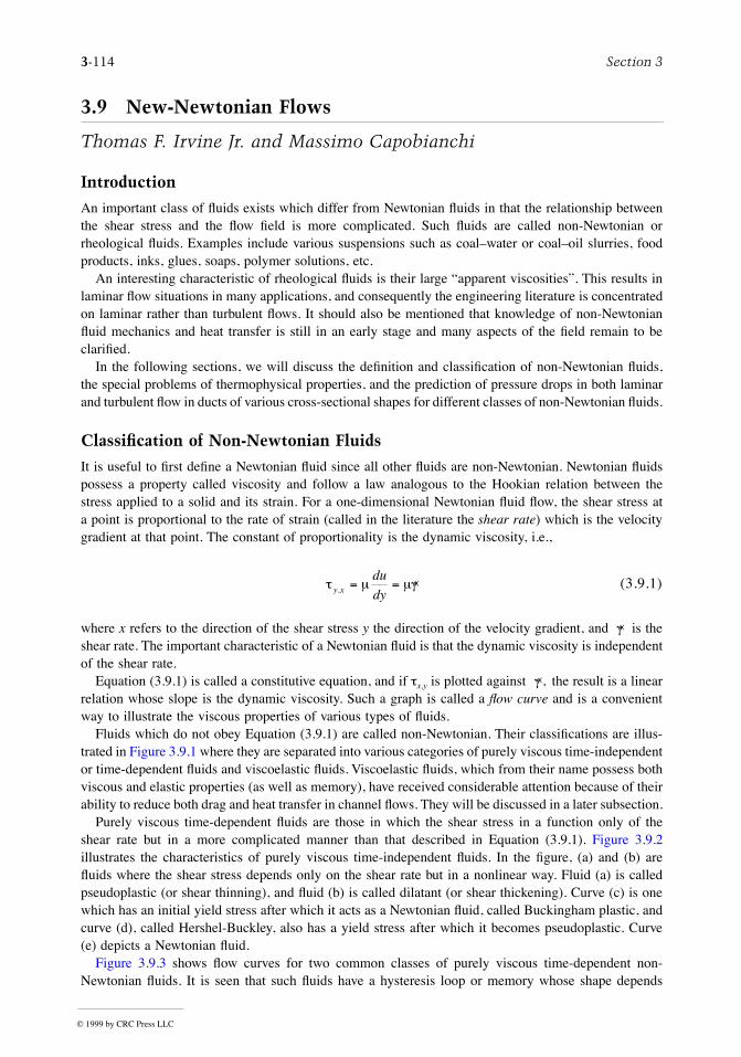
3-114 Section 3
3.9 New-Newtonian Flows
Thomas F. Irvine Jr. and Massimo Capobianchi
Introduction
An important class of ßuids exists which differ from Newtonian ßuids in that the relationship betweenthe shear stress and the ßow Þeld is more complicated. Such ßuids are called non-Newtonian orrheological ßuids. Examples include various suspensions such as coalÐwater or coalÐoil slurries, foodproducts, inks, glues, soaps, polymer solutions, etc.
An interesting characteristic of rheological ßuids is their large Òapparent viscositiesÓ. This results inlaminar ßow situations in many applications, and consequently the engineering literature is concentratedon laminar rather than turbulent ßows. It should also be mentioned that knowledge of non-Newtonianßuid mechanics and heat transfer is still in an early stage and many aspects of the Þeld remain to beclariÞed.
In the following sections, we will discuss the deÞnition and classiÞcation of non-Newtonian ßuids,the special problems of thermophysical properties, and the prediction of pressure drops in both laminarand turbulent ßow in ducts of various cross-sectional shapes for different classes of non-Newtonian ßuids.
Classification of Non-Newtonian Fluids
It is useful to Þrst deÞne a Newtonian ßuid since all other ßuids are non-Newtonian. Newtonian ßuidspossess a property called viscosity and follow a law analogous to the Hookian relation between thestress applied to a solid and its strain. For a one-dimensional Newtonian ßuid ßow, the shear stress ata point is proportional to the rate of strain (called in the literature the shear rate) which is the velocitygradient at that point. The constant of proportionality is the dynamic viscosity, i.e.,
(3.9.1)
where x refers to the direction of the shear stress y the direction of the velocity gradient, and is theshear rate. The important characteristic of a Newtonian ßuid is that the dynamic viscosity is independentof the shear rate.
Equation (3.9.1) is called a constitutive equation, and if tx,y is plotted against , the result is a linearrelation whose slope is the dynamic viscosity. Such a graph is called a ßow curve and is a convenientway to illustrate the viscous properties of various types of ßuids.
Fluids which do not obey Equation (3.9.1) are called non-Newtonian. Their classiÞcations are illus-trated in Figure 3.9.1 where they are separated into various categories of purely viscous time-independentor time-dependent ßuids and viscoelastic ßuids. Viscoelastic ßuids, which from their name possess bothviscous and elastic properties (as well as memory), have received considerable attention because of theirability to reduce both drag and heat transfer in channel ßows. They will be discussed in a later subsection.
Purely viscous time-dependent ßuids are those in which the shear stress in a function only of theshear rate but in a more complicated manner than that described in Equation (3.9.1). Figure 3.9.2illustrates the characteristics of purely viscous time-independent ßuids. In the Þgure, (a) and (b) areßuids where the shear stress depends only on the shear rate but in a nonlinear way. Fluid (a) is calledpseudoplastic (or shear thinning), and ßuid (b) is called dilatant (or shear thickening). Curve (c) is onewhich has an initial yield stress after which it acts as a Newtonian ßuid, called Buckingham plastic, andcurve (d), called Hershel-Buckley, also has a yield stress after which it becomes pseudoplastic. Curve(e) depicts a Newtonian ßuid.
Figure 3.9.3 shows ßow curves for two common classes of purely viscous time-dependent non-Newtonian ßuids. It is seen that such ßuids have a hysteresis loop or memory whose shape depends
t m mgy x
du
dy,Ç= =
Çg
Çg
© 1999 by CRC Press LLC
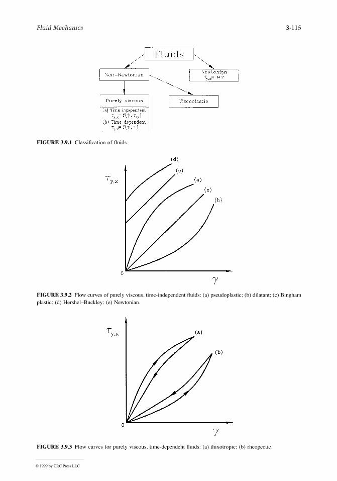
Fluid Mechanics 3-115
FIGURE 3.9.1 ClassiÞcation of ßuids.
FIGURE 3.9.2 Flow curves of purely viscous, time-independent ßuids: (a) pseudoplastic; (b) dilatant; (c) Binghamplastic; (d) HershelÐBuckley; (e) Newtonian.
FIGURE 3.9.3 Flow curves for purely viscous, time-dependent ßuids: (a) thixotropic; (b) rheopectic.
© 1999 by CRC Press LLC

3-116 Section 3
upon the time-dependent rate at which the shear stress is applied. Curve (a) illustrates a pseudoplastictime-dependent ßuid and curve (b) a dilatant time-dependent ßuid. They are called, respectively, thixo-tropic and rheopectic ßuids and are complicated by the fact that their ßow curves are difÞcult tocharacterize for any particular application.
Apparent Viscosity
Although non-Newtonian ßuids do not have the property of viscosity, in the Newtonian ßuid sense, itis convenient to deÞne an apparent viscosity which is the ratio of the local shear stress to the shear rateat that point.
(3.9.2)
The apparent viscosity is not a true property for non-Newtonian ßuids because its value depends uponthe ßow Þeld, or shear rate. Nevertheless, it is a useful quantity and ßow curves are often constructedwith the apparent viscosity as the ordinate and shear rate as the abscissa. Such a ßow curve will beillustrated in a later subsection.
Constitutive Equations
A constitutive equation is one that expresses the relation between the shear stress or apparent viscosityand the shear rate through the rheological properties of the ßuid. For example, Equation (3.9.1) is theconstitutive equation for a Newtonian ßuid.
Many constitutive equations have been developed for non-Newtonian ßuids with some of them havingas many as Þve rheological properties. For engineering purposes, simpler equations are normally satis-factory and two of the most popular will be considered here.
Since many of the non-Newtonian ßuids in engineering applications are pseudoplastic, such ßuidswill be used in the following to illustrate typical ßow curves and constitutive equations. Figure 3.9.4 isa qualitative ßow curve for a typical pseudoplastic ßuid plotted with logarithmic coordinates. It is seenin the Þgure that at low shear rates, region (a), the ßuid is Newtonian with a constant apparent viscosityof mo (called the zero shear rate viscosity). At higher shear rates, region (b), the apparent viscosity beginsto decrease until it becomes a straight line, region (c). This region (c) is called the power law regionand is an important region in ßuid mechanics and heat transfer. At higher shear rates than the powerlaw region, there is another transition region (d) until again the ßuid becomes Newtonian in region (e).As discussed below, regions (a), (b), and (c) are where most of the engineering applications occur.
FIGURE 3.9.4 Illustrative ßow curve for a pseudoplastic ßuid (a) Newtonian region; (b) transition region I: (c)power law region; (d) transition region II; (e) high-shear-rate Newtonian region.
mtga =Ç
© 1999 by CRC Press LLC
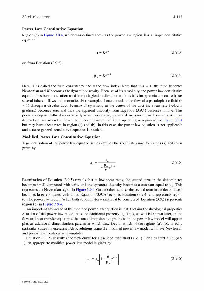
Fluid Mechanics 3-117
Power Law Constitutive Equation
Region (c) in Figure 3.9.4, which was deÞned above as the power law region, has a simple constitutiveequation:
(3.9.3)
or, from Equation (3.9.2):
(3.9.4)
Here, K is called the ßuid consistency and n the ßow index. Note that if n = 1, the ßuid becomesNewtonian and K becomes the dynamic viscosity. Because of its simplicity, the power law constitutiveequation has been most often used in rheological studies, but at times it is inappropriate because it hasseveral inherent ßaws and anomalies. For example, if one considers the ßow of a pseudoplastic ßuid (n< 1) through a circular duct, because of symmetry at the center of the duct the shear rate (velocitygradient) becomes zero and thus the apparent viscosity from Equation (3.9.4) becomes inÞnite. Thisposes conceptual difÞculties especially when performing numerical analyses on such systems. AnotherdifÞculty arises when the ßow Þeld under consideration is not operating in region (c) of Figure 3.9.4but may have shear rates in region (a) and (b). In this case, the power law equation is not applicableand a more general constitutive equation is needed.
Modified Power Law Constitutive Equation
A generalization of the power law equation which extends the shear rate range to regions (a) and (b) isgiven by
(3.9.5)
Examination of Equation (3.9.5) reveals that at low shear rates, the second term in the denominatorbecomes small compared with unity and the apparent viscosity becomes a constant equal to mO. Thisrepresents the Newtonian region in Figure 3.9.4. On the other hand, as the second term in the denominatorbecomes large compared with unity, Equation (3.9.5) becomes Equation (3.9.4) and represents region(c), the power law region. When both denominator terms must be considered, Equation (3.9.5) representsregion (b) in Figure 3.9.4.
An important advantage of the modiÞed power law equation is that it retains the rheological propertiesK and n of the power law model plus the additional property mo. Thus, as will be shown later, in theßow and heat transfer equations, the same dimensionless groups as in the power law model will appearplus an additional dimensionless parameter which describes in which of the regions (a), (b), or (c) aparticular system is operating. Also, solutions using the modiÞed power law model will have Newtonianand power law solutions as asymptotes.
Equation (3.9.5) describes the ßow curve for a pseudoplastic ßuid (n < 1). For a dilatant ßuid, (n >1), an appropriate modiÞed power law model is given by
(3.9.6)
t g= K nÇ
m ganK= -Ç 1
mmm
ga
o
o n
K
=+ -1 1Ç
m mm
ga oo
nK= +
é
ëê
ù
ûú
-1 1Ç
© 1999 by CRC Press LLC
3-118 Section 3
Many other constitutive equations have been proposed in the literature (Skelland, 1967; Cho and Hartnett,1982; Irvine and Karni, 1987), but the ones discussed above are sufÞcient for a large number ofengineering applications and agree well with the experimental determinations of rheological properties.
Rheological Property Measurements
For non-Newtonian ßuids, specifying the appropriate rheological properties for a particular ßuid isformidable because such ßuids are usually not pure substances but various kinds of mixtures. This meansthat the properties are not available in handbooks or other reference materials but must be measured foreach particular application. A discussion of the various instruments for measuring rheological propertiesis outside the scope of the present section, but a number of sources are available which describe differentrheological property measurement techniques and instruments: Skelland (1967), Whorlow (1980), Irvineand Karni (1987), and Darby (1988). Figure 3.9.5 is an illustration of experimental ßow curves measuredwith a falling needle viscometer and a square duct viscometer for polymer solutions of differentconcentrations. Also known in the Þgure as solid lines is the modiÞed power law equation used torepresent the experimental data. It is seen that Equation (3.9.5) Þts the experimental data within ±2%.Table 3.9.1 lists the rheological properties used in the modiÞed power law equations in Figure 3.9.5. Itmust be emphasized that a proper knowledge of these properties is vital to the prediction of ßuidmechanics and heat transfer phenomena in rheological ßuids.
Fully Developed Laminar Pressure Drops for Time-Independent Non-Newtonian Fluids
Modified Power Law Fluids
This important subject will be considered by Þrst discussing modiÞed power law ßuids. The reason isthat such solutions include both friction factorÐReynolds number relations and a shear rate parameter.The latter allows the designer to determine the shear rate region in which his system is operating andthus the appropriate solution to be used, i.e., regions (a), (b), or (c) in Figure 3.9.4.
For laminar fully developed ßow of a modiÞed power law ßuid in a circular duct, the product of thefriction factor and a certain Reynolds number is a constant depending on the ßow index, n, and the shearrate parameter, b.
(3.9.7)
where fD is the Darcy friction factor and Rem the modiÞed power law Reynolds number, i.e.,
(Darcy friction factor)*
* It should be noted that the Fanning friction factor is also used in the technical literature. The Fanning frictionfactor is 1/4 of the Darcy friction factor, and will be characterized by the symbol fF.
TABLE 3.9.1 Rheological Properties Used in the ModiÞed Power Law Equations in Figure 3.9.5 for Three Polymer Solutions of CMC-7H4
CMC K (N á secn/m2) n mo (N á sec/m2)n
5000 wppm 2.9040 0.3896 0.214882500 wppm 1.0261 0.4791 0.064541500 wppm 0.5745 0.5204 0.03673
Source: Park, S. et al., Proc. Third World Conf. Heat Transfer, Fluid Mechanics, and Thermodynamics, Vol. 1, Elsevier, New York, 1993, 900Ð908.
f nD m× = ( )Re constant ,b
f
p
LD
uD
H
=2
2
D
r
© 1999 by CRC Press LLC
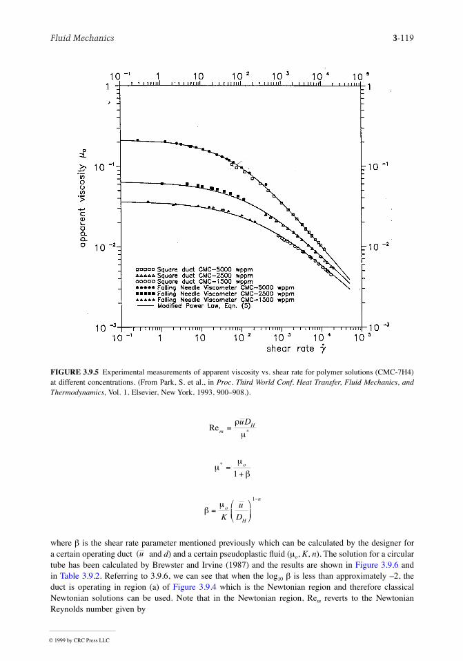
Fluid Mechanics 3-119
where b is the shear rate parameter mentioned previously which can be calculated by the designer fora certain operating duct and d) and a certain pseudoplastic ßuid (mo, K, n). The solution for a circulartube has been calculated by Brewster and Irvine (1987) and the results are shown in Figure 3.9.6 andin Table 3.9.2. Referring to 3.9.6, we can see that when the log10 b is less than approximately Ð2, theduct is operating in region (a) of Figure 3.9.4 which is the Newtonian region and therefore classicalNewtonian solutions can be used. Note that in the Newtonian region, Rem reverts to the NewtonianReynolds number given by
FIGURE 3.9.5 Experimental measurements of apparent viscosity vs. shear rate for polymer solutions (CMC-7H4)at different concentrations. (From Park, S. et al., in Proc. Third World Conf. Heat Transfer, Fluid Mechanics, andThermodynamics, Vol. 1, Elsevier, New York, 1993, 900Ð908.).
RemHuD
=r
m*
mm
b* =
+o
1
bm
=æ
èç
ö
ø÷
-
o
H
n
K
u
D
1
(u
© 1999 by CRC Press LLC
3-120 Section 3
FIGURE 3.9.6 Product of friction factor and modiÞed Reynolds number vs. log10 b for a circular duct. .
TABLE 3.9.2 Summary of Computed Values of fD á Rem for Various Values of n and b for a Circular Duct
fD á Rem for Flow Index: n =
b 1.0 0.9 0.8 0.7 0.6 0.5
10Ð5 64.000 64.000 64.000 64.000 63.999 63.999
10Ð4 64.000 63.999 63.997 63.995 63.993 63.990
10Ð3 64.000 63.987 63.972 63.953 63.930 63.903
10Ð2 64.000 63.873 63.720 63.537 63.318 63.055
10Ð1 64.000 62.851 61.519 59.987 58.237 56.243
100 64.000 58.152 52.377 46.761 41.384 36.299
101 64.000 54.106 45.597 38.308 32.082 26.771
102 64.000 53.371 44.458 36.985 30.716 25.451
103 64.000 53.291 44.336 36.845 30.573 25.314
104 64.000 53.283 44.324 36.831 30.559 25.300
105 64.000 53.282 44.323 36.830 30.557 25.299
Exact solution 64.000 53.282 44.323 36.829 30.557 25.298
Source: Brewster, R.A. and Irvine, T.F., Jr., W�rme und Stoff�bertragung, 21, 83Ð86, 1987. With permission.
-4
70
60
50
40
30
20-3 -2 -1 0 1 2 3 4
64.0
53.282
44.323
36.829
30.557
25.299
n = 1.0
0.9
0.8
0.7
0.6
0.5
log b
f D×R
e m
© 1999 by CRC Press LLC
Fluid Mechanics 3-121
(3.9.8)
When the value of log10 b is approximately in the range Ð2 £ log10 b £ 2, the duct is operating in thetransition region (b) of Figure 3.9.4 and the values of fD á Rem must be obtained from Figure 3.9.6 orfrom Table 3.9.2.
When log10 b is greater than approximately 2, the duct is operating in the power law region (c) ofFigure 3.9.4 and power law friction factor Reynolds number relations can be used. They are also indicatedin Figure 3.9.6 and Table 3.9.2. In this region, Rem becomes the power law Reynolds number given by
(3.9.9)
For convenience, Brewster and Irvine (1987) have presented a correlation equation which agrees within0.1% with the results tabulated in Table 3.9.2.
(3.9.10)
Thus, Equation (3.9.10) contains all of the information required to calculate the circular tube laminarfully developed pressure drop for a pseudoplastic ßuid depending upon the shear rate region(s) underconsideration, i.e., regions (a), (b), or (c) of Figure 3.9.4. Note that in scaling such non-Newtoniansystems, both Rem and b must be held constant. ModiÞed power law solutions have been reported fortwo other duct shapes. Park et al. (1993) have presented the friction factorÐReynolds number relationsfor rectangular ducts and Capobianchi and Irvine (1992) for concentric annular ducts.
Power Law Fluids
Since the power law region of modiÞed power law ßuids (log10 b ³ 2) is often encountered, the frictionfactorÐReynolds number relations will be discussed in detail in this subsection.
An analysis of power law ßuids which is most useful has been presented by Kozicki et al. (1967).Although the method is approximate, its overall accuracy (±5%) is usually sufÞcient for many engineeringcalculations. His expression for the friction factorÐReynolds number product is given by
(3.9.11)
where
(3.9.12)
and a and b are geometric constants which depend on the cross-sectional shape of the duct. For example,for a circular duct, a = 0.25 and b = 0.75. Values of a and b for other duct shapes are tabulated in Table3.9.3. For additional duct shapes in both closed and open channel ßows, Kozicki et al. (1967) may beconsulted.
ReNH
o
uD=
r
m
Reg
nHnu D
K=
-r 2
f
n
n
D m
nn
× =+
++æ
èöø
+
Re1
164
23 1
43 3
bb
fDn× =Re* 26
Re Kozicki Reynolds number, ReRe
* *= =+é
ëêùûú
-
gn
na bn
n8 1
© 1999 by CRC Press LLC
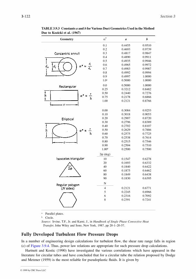
3-122 Section 3
Fully Developed Turbulent Flow Pressure Drops
In a number of engineering design calculations for turbulent ßow, the shear rate range falls in region(c) of Figure 3.9.4. Thus, power law relations are appropriate for such pressure drop calculations.
Hartnett and Kostic (1990) have investigated the various correlations which have appeared in theliterature for circular tubes and have concluded that for a circular tube the relation proposed by Dodgeand Metzner (1959) is the most reliable for pseudoplastic ßuids. It is given by
TABLE 3.9.3 Constants a and b for Various Duct Geometrics Used in the Method Due to Kozicki et al. (1967)
Geometry a* a b
0.1 0.4455 0.95100.2 0.4693 0.97390.3 0.4817 0.98470.4 0.4890 0.99110.5 0.4935 0.99460.6 0.4965 0.99720.7 0.4983 0.99870.8 0.4992 0.99940.9 0.4997 1.00001.0a 0.5000 1.0000
0.0 0.5000 1.00000.25 0.3212 0.84820.50 0.2440 0.72760.75 0.2178 0.68661.00 0.2121 0.8766
0.00 0.3084 0.92530.10 0.3018 0.90530.20 0.2907 0.87200.30 0.2796 0.83890.40 0.2702 0.81070.50 0.2629 0.78860.60 0.2575 0.77250.70 0.2538 0.76140.80 0.2515 0.75460.90 0.2504 0.75101.00b 0.2500 0.7500
2f (deg)
10 0.1547 0.627820 0.1693 0.633240 0.1840 0.642260 0.1875 0.646280 0.1849 0.643890 0.1830 0.6395
N
4 0.2121 0.67715 0.2245 0.69666 0.2316 0.70928 0.2391 0.7241
a Parallel plates.b Circle.Source: Irvine, T.F., Jr. and Karni, J., in Handbook of Single Phase Convective Heat Transfer, John Wiley and Sons, New York, 1987, pp 20-1Ð20-57.
© 1999 by CRC Press LLC
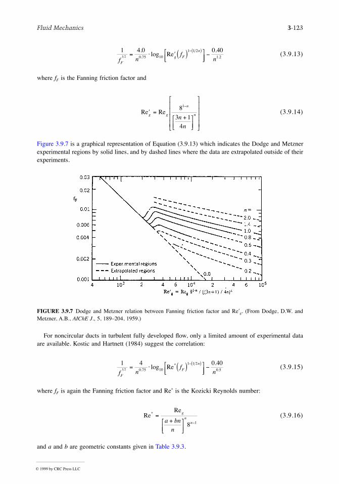
Fluid Mechanics 3-123
(3.9.13)
where fF is the Fanning friction factor and
(3.9.14)
Figure 3.9.7 is a graphical representation of Equation (3.9.13) which indicates the Dodge and Metznerexperimental regions by solid lines, and by dashed lines where the data are extrapolated outside of theirexperiments.
For noncircular ducts in turbulent fully developed ßow, only a limited amount of experimental dataare available. Kostic and Hartnett (1984) suggest the correlation:
(3.9.15)
where fF is again the Fanning friction factor and Re* is the Kozicki Reynolds number:
(3.9.16)
and a and b are geometric constants given in Table 3.9.3.
FIGURE 3.9.7 Dodge and Metzner relation between Fanning friction factor and Re¢g. (From Dodge, D.W. andMetzner, A.B., AIChE J., 5, 189Ð204, 1959.)
1 4 0 0 401 2 0 75 10
1 1 2
1 2f n
fn
F
g F
n= × ¢ ( )é
ëêùûú
--( ).
log.
. .Re
Re Re¢ =+é
ëêùûú
é
ë
êêêê
ù
û
úúúú
-
g g
n
nn
n
8
3 14
1
1 4 0 401 2 0 75 10
1 1 2
0 5f n
fn
F
F
n= × ( )é
ëêùûú
--( )
. .log.
Re*
ReRe
* =+é
ëêùûú
-
gn
na bn
n8 1
© 1999 by CRC Press LLC
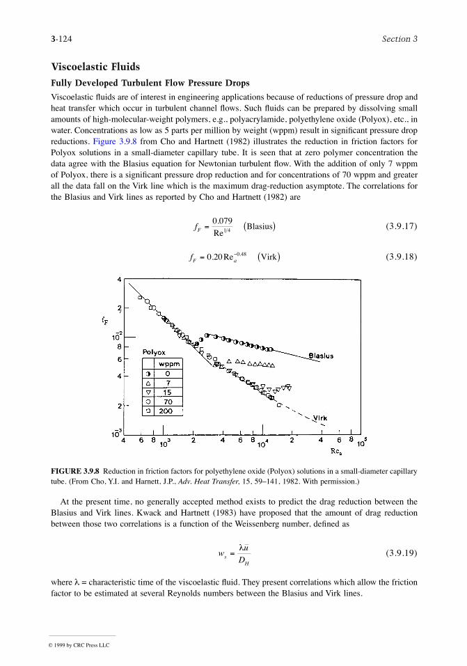
3-124 Section 3
Viscoelastic Fluids
Fully Developed Turbulent Flow Pressure Drops
Viscoelastic ßuids are of interest in engineering applications because of reductions of pressure drop andheat transfer which occur in turbulent channel ßows. Such ßuids can be prepared by dissolving smallamounts of high-molecular-weight polymers, e.g., polyacrylamide, polyethylene oxide (Polyox), etc., inwater. Concentrations as low as 5 parts per million by weight (wppm) result in signiÞcant pressure dropreductions. Figure 3.9.8 from Cho and Hartnett (1982) illustrates the reduction in friction factors forPolyox solutions in a small-diameter capillary tube. It is seen that at zero polymer concentration thedata agree with the Blasius equation for Newtonian turbulent ßow. With the addition of only 7 wppmof Polyox, there is a signiÞcant pressure drop reduction and for concentrations of 70 wppm and greaterall the data fall on the Virk line which is the maximum drag-reduction asymptote. The correlations forthe Blasius and Virk lines as reported by Cho and Hartnett (1982) are
(3.9.17)
(3.9.18)
At the present time, no generally accepted method exists to predict the drag reduction between theBlasius and Virk lines. Kwack and Hartnett (1983) have proposed that the amount of drag reductionbetween those two correlations is a function of the Weissenberg number, deÞned as
(3.9.19)
where l = characteristic time of the viscoelastic ßuid. They present correlations which allow the frictionfactor to be estimated at several Reynolds numbers between the Blasius and Virk lines.
FIGURE 3.9.8 Reduction in friction factors for polyethylene oxide (Polyox) solutions in a small-diameter capillarytube. (From Cho, Y.I. and Harnett, J.P., Adv. Heat Transfer, 15, 59Ð141, 1982. With permission.)
fF = ( )0 0791 4
.Re
Blasius
fF a= ( )-0 20 0 48. .Re Virk
wu
DsH
=l
© 1999 by CRC Press LLC
Fluid Mechanics 3-125
Fully Developed Laminar Flow Pressure Drops
The above discussion on viscoelastic ßuids has only considered fully developed turbulent ßows. Laminarfully developed ßows can be considered as nonviscoelastic but purely viscous non-Newtonian. Therefore,the method of Kozicki et al. (1967) may be applied to such situations once the appropriate rheologicalproperties have been determined.
Nomenclaturea = duct shape geometric constantb = duct shape geometric constantc = duct width (see Table 3.9.3) (m)di = concentric annuli inner diameter (see Table 3.9.3) (m)do = concentric annuli outer diameter (see Table 3.9.3) (m)fD = Darcy friction factorfF = Fanning friction factorh = duct height (see Table 3.9.3) (m)K = ßuid consistency (Nsn/m2)n = ßow indexN = number of sides in polygon (see Table 3.9.3)
Reg = generalized Reynolds number,
Rem = modiÞed power law Reynolds number,
ReN = modiÞed power law Reynolds number Newtonian asymptote,
Rea = apparent Reynolds number
Re* = Kozicki Reynolds number
Reg
nHnu D
K=
-r 2
RemHuD
=r
m*
ReNH
o
uD=
r
m
ReRe
agn
nn
n
=+æ
èöø
--3 1
48
11
Re* =+é
ëêùûú
-
-
ru D
Ka bn
n
nHn
nn
2
18
© 1999 by CRC Press LLC
3-126 Section 3
= Metzner Reynolds number
= average streamwise velocity (m/sec)t = time (sec)
ws = Weissenberg numberx = direction of shear stress (m)y = direction of velocity gradient (m)
Greek
a* = duct aspect ratio in Table 3.9.3b = shear rate parameter
= shear rate (L/sec)DP = presure drop (N/m2)
l = characteristic time of viscoelastic ßuid (sec)ma = apparent viscosity (N á sec/m2)mo = zero shear rate viscosity (N á sec/m2)m¥ = high shear rate viscosity (N á sec/m2)m* = reference viscosity
to = yield stress (N/m2)ty,x = shear stress (N/m2)
f = half apex angle (see Table 3.9.3) (°)
References
Brewster, A.A. and Irvine, T.F. Jr. 1987. Similtude considerations in laminar ßow of power law ßuidsin circular ducts, W�rme und Stoff�bertagung, 21:83Ð86.
Capobianchi, M. and Irvine, T.F. Jr. 1992. Predictions of pressure drop and heat transfer in concentricannular ducts with modiÞed power law ßuids, W�rme und Stoff�bertagung, 27:209Ð215.
Cho, Y.I. and Hartnett, J.P. 1982. Non-Newtonian ßuids in circular pipe ßow, in Adv. Heat Transfer,15:59Ð141.
Darby, R. 1988. Laminar and turbulent pipe ßows of non-Newtonian ßuids, in Encyclopedia of FluidMechanics, Vol. 7, Gulf Publishing, Houston, 7:20Ð53.
Dodge, D.W. and Metzner, A.B. 1959. Turbulent ßow of non-Newtonian systems, AIChE J., 5:189Ð204.Harnett, J.P. and Kostic, M. 1990. Turbulent Friction Factor Correlations for Power Law Fluids in Circular
and Non-Circular Channels, Int. Comm. Heat and Mass Transfer, 17:59Ð65.
Re¢g
Re Re¢ =+é
ëêùûú
é
ë
êêêê
ù
û
úúúú
-
g g
n
nn
n
8
3 14
1
u
bm
=æ
èç
ö
ø÷
-
o
H
n
K
u
D
1
Çg
mm
b* 2N sec m=
+×( )o
1
© 1999 by CRC Press LLC
Fluid Mechanics 3-127
Irvine, T.F. Jr. and Karni, J. 1987. Non-Newtonian ßuid ßow and heat transfer, in Handbook of SinglePhase Convective Heat Transfer, pp. 20-1Ð20-57, John Wiley and Sons, New York.
Kostic, M. and Hartnett, J.P. 1984. Predicting turbulent friction factors of non-Newtonian ßuids in non-circular ducts, Int. Comm. Heat and Mass Transfer, 11:345Ð352.
Kozicki, W., Chou, C.H., and Tiu, C. 1967. Non-Newtonian ßow in ducts of arbitrary cross-sectionalshape, Can. J. Chem. Eng., 45:127Ð134.
Kwack, E.Y. and Hartnett, J.P. 1983. Empirical correlations of turbulent friction factors and heat transfercoefÞcients for viscoelastic ßuids, Int. Comm. Heat and Mass Transfer, 10:451Ð461.
Park, S., Irvine, T.F. Jr., and Capobianchi, M. 1993. Experimental and numerical study of friction factorfor a modiÞed power law ßuid in a rectangular duct, Proc. Third World Conf. Heat Transfer, FluidMechanics, and Thermodynamics, Vol. 1, Elsevier, New York, 1:900Ð908.
Skelland, A.H.P. 1967. Non-Newtonian Flow and Heat Transfer, John Wiley and Sons, New York.Whorlow, R.W. 1980. Rheological Techniques, Halsted Press, New York.
Further Information
It is not possible to include all of the interesting non-Newtonian topics in a section of this scope. Otheritems which may be of interest and importance are listed below along with appropriate references:hydrodynamic and thermal entrance lengths, Cho and Hartnett (1982); non-Newtonian ßow over externalsurfaces, Irvine and Karni (1987); chemical, solute, and degradation effects in viscoelastic ßuids, Choand Harnett (1982); general references, Skelland (1967), Whorlow (1980), and Darby (1988).
© 1999 by CRC Press LLC
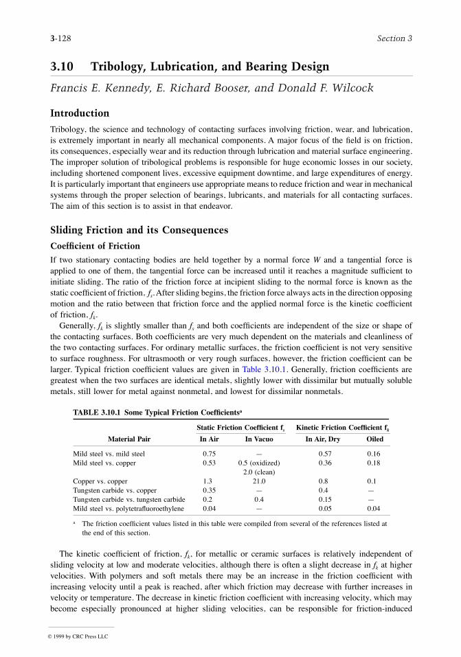
3-128 Section 3
3.10 Tribology, Lubrication, and Bearing Design
Francis E. Kennedy, E. Richard Booser, and Donald F. Wilcock
Introduction
Tribology, the science and technology of contacting surfaces involving friction, wear, and lubrication,is extremely important in nearly all mechanical components. A major focus of the Þeld is on friction,its consequences, especially wear and its reduction through lubrication and material surface engineering.The improper solution of tribological problems is responsible for huge economic losses in our society,including shortened component lives, excessive equipment downtime, and large expenditures of energy.It is particularly important that engineers use appropriate means to reduce friction and wear in mechanicalsystems through the proper selection of bearings, lubricants, and materials for all contacting surfaces.The aim of this section is to assist in that endeavor.
Sliding Friction and its Consequences
Coefficient of Friction
If two stationary contacting bodies are held together by a normal force W and a tangential force isapplied to one of them, the tangential force can be increased until it reaches a magnitude sufÞcient toinitiate sliding. The ratio of the friction force at incipient sliding to the normal force is known as thestatic coefÞcient of friction, fs. After sliding begins, the friction force always acts in the direction opposingmotion and the ratio between that friction force and the applied normal force is the kinetic coefÞcientof friction, fk.
Generally, fk is slightly smaller than fs and both coefÞcients are independent of the size or shape ofthe contacting surfaces. Both coefÞcients are very much dependent on the materials and cleanliness ofthe two contacting surfaces. For ordinary metallic surfaces, the friction coefÞcient is not very sensitiveto surface roughness. For ultrasmooth or very rough surfaces, however, the friction coefÞcient can belarger. Typical friction coefÞcient values are given in Table 3.10.1. Generally, friction coefÞcients aregreatest when the two surfaces are identical metals, slightly lower with dissimilar but mutually solublemetals, still lower for metal against nonmetal, and lowest for dissimilar nonmetals.
The kinetic coefÞcient of friction, fk, for metallic or ceramic surfaces is relatively independent ofsliding velocity at low and moderate velocities, although there is often a slight decrease in fk at highervelocities. With polymers and soft metals there may be an increase in the friction coefÞcient withincreasing velocity until a peak is reached, after which friction may decrease with further increases invelocity or temperature. The decrease in kinetic friction coefÞcient with increasing velocity, which maybecome especially pronounced at higher sliding velocities, can be responsible for friction-induced
TABLE 3.10.1 Some Typical Friction CoefÞcientsa
Static Friction CoefÞcient fs Kinetic Friction CoefÞcient fk
Material Pair In Air In Vacuo In Air, Dry Oiled
Mild steel vs. mild steel 0.75 Ñ 0.57 0.16Mild steel vs. copper 0.53 0.5 (oxidized) 0.36 0.18
2.0 (clean)Copper vs. copper 1.3 21.0 0.8 0.1Tungsten carbide vs. copper 0.35 Ñ 0.4 ÑTungsten carbide vs. tungsten carbide 0.2 0.4 0.15 ÑMild steel vs. polytetraßuoroethylene 0.04 Ñ 0.05 0.04
a The friction coefÞcient values listed in this table were compiled from several of the references listed at the end of this section.
© 1999 by CRC Press LLC
Fluid Mechanics 3-129
vibrations (stickÐslip oscillations) of the sliding systems. Such vibrations are an important designconsideration for clutches and braking systems, and can also be important in the accurate control andpositioning of robotic mechanisms and precision manufacturing systems.
Wear
Wear is the unwanted removal of material from solid surfaces by mechanical means; it is one of theleading reasons for the failure and replacement of manufactured products. It has been estimated that thecosts of wear, which include repair and replacement, along with equipment downtime, constitute up to6% of the U.S. gross national product (Rabinowicz, 1995). Wear can be classiÞed into four primarytypes: sliding wear, abrasion, erosion, and corrosive wear. Owing to its importance, wear and its controlhave been the subject of several handbooks (Peterson and Winer, 1980; Blau, 1992), which the interestedreader may consult for further information.
Types of Wear. Sliding wear occurs to some degree whenever solid surfaces are in sliding contact. Thereare two predominant sliding wear mechanisms, adhesion and surface fatigue. Adhesive wear is causedby strong adhesive forces between the two surfaces within the real area of contact. It results in theremoval of small particles from at least one of the surfaces, usually the softer one. These particles canthen transfer to the other surface or mix with other material from both surfaces before being expelledas loose wear debris. Adhesive wear can be particularly severe for surfaces which have a strong afÞnityfor each other, such as those made from identical metals. Surface fatigue wear occurs when repeatedsliding or rolling/sliding over a wear track results in the initiation of surface or subsurface cracks, andthe propagation of those cracks produces wear particles in ductile materials by a process that has beencalled delamination. With brittle materials, sliding wear often occurs by a surface fracture process.
After an initial transition or Òrunning-inÓ period, sliding wear tends to reach a steady state rate whichis approximated by the following Archard (or Holm/Archard) wear equation:
(3.10.1)
where V = volume of worn material, K = dimensionless wear coefÞcient, s = sliding distance, W =normal load between the surfaces, and H = hardness of the softer of the two contacting surfaces.
The dimensionless wear coefÞcient gives an indication of the tendency of a given material combinationto wear; relative wear coefÞcient values are given in Figure 3.10.1. In general, wear coefÞcients arehighest for identical metals sliding without lubrication, and wear is decreased by adding a lubricant andby having material pairs which are dissimilar.
Abrasive wear occurs when a hard, rough surface slides against a softer surface (two-body abrasion)or when hard particles slide between softer surfaces (three-body abrasion). This process usually resultsin material removal by plowing or chip formation, especially when the abraded surface is metallic;surface fracture can occur during abrasion of brittle surfaces. In fact, abrasion mechanisms are similarto those of grinding and lapping, which could be considered as intentional abrasion. Consideration ofthe cutting and plowing processes shows that abrasive wear obeys the same equation (3.10.1) as slidingwear (Archard, 1980; Rabinowicz, 1995). Typical wear coefÞcients for abrasive wear are given in Figure3.10.1. Since the relative size, hardness, and sharpness of the abrading particles, or surface asperities,also affect abrasive wear rates, the wear coefÞcients for abrasion must include recognition of thosefactors (Rabinowicz, 1995).
Erosion occurs when solid particles or liquid droplets impinge on a solid surface. When impingementis on a ductile metallic surface, the wear process is similar to that caused by abrasion, and is dominatedby plastic deformation. Brittle surfaces, on the other hand, tend to erode by surface fracture mechanisms.The material removal rate is dependent on the angle of attack of the particles, with erosion reaching apeak at low angles (about 20°) for ductile surfaces and at high angles (90°) for brittle materials. In eithercase, the wear rate is proportional to the mass rate of ßow of the particles and to their kinetic energy;it is inversely proportional to the hardness of the surface and the energy-absorbing potential (or toughness)
V K W s H= * *
© 1999 by CRC Press LLC
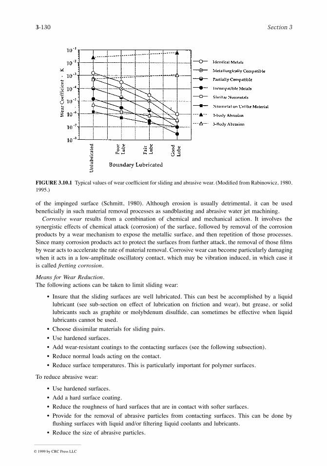
3-130 Section 3
of the impinged surface (Schmitt, 1980). Although erosion is usually detrimental, it can be usedbeneÞcially in such material removal processes as sandblasting and abrasive water jet machining.
Corrosive wear results from a combination of chemical and mechanical action. It involves thesynergistic effects of chemical attack (corrosion) of the surface, followed by removal of the corrosionproducts by a wear mechanism to expose the metallic surface, and then repetition of those processes.Since many corrosion products act to protect the surfaces from further attack, the removal of those Þlmsby wear acts to accelerate the rate of material removal. Corrosive wear can become particularly damagingwhen it acts in a low-amplitude oscillatory contact, which may be vibration induced, in which case itis called fretting corrosion.
Means for Wear Reduction.The following actions can be taken to limit sliding wear:
¥ Insure that the sliding surfaces are well lubricated. This can best be accomplished by a liquidlubricant (see sub-section on effect of lubrication on friction and wear), but grease, or solidlubricants such as graphite or molybdenum disulÞde, can sometimes be effective when liquidlubricants cannot be used.
¥ Choose dissimilar materials for sliding pairs.
¥ Use hardened surfaces.
¥ Add wear-resistant coatings to the contacting surfaces (see the following subsection).
¥ Reduce normal loads acting on the contact.
¥ Reduce surface temperatures. This is particularly important for polymer surfaces.
To reduce abrasive wear:
¥ Use hardened surfaces.
¥ Add a hard surface coating.
¥ Reduce the roughness of hard surfaces that are in contact with softer surfaces.
¥ Provide for the removal of abrasive particles from contacting surfaces. This can be done byßushing surfaces with liquid and/or Þltering liquid coolants and lubricants.
¥ Reduce the size of abrasive particles.
FIGURE 3.10.1 Typical values of wear coefÞcient for sliding and abrasive wear. (ModiÞed from Rabinowicz, 1980,1995.)
© 1999 by CRC Press LLC
Fluid Mechanics 3-131
To reduce erosion:
¥ Modify the angle of impingement of solid particles or liquid droplets.
¥ Provide for the removal of solid particles from the stream of ßuid.
¥ Use hardened surfaces.
¥ Use tough materials for surfaces.
¥ Add protective coating to surfaces.
Surface Engineering for Friction and Wear Reduction
Surface treatments have long been an important remedy for wear problems, and that importance hasgrown in recent years with the introduction of new techniques to harden surfaces or apply hard surfacecoatings. Available processes and characteristics for treating a steel substrate are listed in Table 3.10.2.
Thermal transformation hardening processes are used to harden ferrous (primarily steel) surfaces byheating the surface rapidly, transforming it to austenite, and then quenching it to form martensite. Thesource of heat can be one of the following: an oxyacetylene or oxypropane ßame (ßame hardening),eddy currents induced by a high-frequency electric Þeld (induction hardening), a beam from a high-power laser (laser hardening), or a focused electron beam (electron beam hardening). The depth anduniformity of the hard layer depend on the rate and method of heating. These processes are characterizedby a short process time and all except electron beam hardening (which requires a moderate vacuum)can be done in air.
Thermal diffusion processes involve the diffusion of atoms into surfaces to create a hard layer. In themost widely used of these processes, carburizing (or case hardening), carbon diffuses into a low-carbonsteel surface to produce a hard, carbon-rich case. The hardness and thickness of the case depend on thetemperature, exposure time, and source of carbon (either a hydrocarbon gas, a salt bath, or a packed bedof carbon). Carbonitriding is a process similar to carburizing which involves the simultaneous diffusionof carbon and nitrogen atoms into carbon steel surfaces. In the nitriding process, nitrogen atoms diffuseinto the surface of a steel which contains nitride-forming elements (such as Al, Cr, Mo, V, W, or Ti) andform Þne precipitates of nitride compounds in a near-surface layer. The hardness of the surface layerdepends on the types of nitrides formed. The source of nitrogen can be a hot gas (usually ammonia) ora plasma. Nitrocarburizing and boronizing are related processes in which nitrogen or boron atoms diffuse
TABLE 3.10.2 Characteristics of Surface Treatment Processes for Steel
Coating or Treated Layer
Substrate Temperature(°C)Process Hardness (HV)
Thickness (mm)
Surface hardeningFlame or induction hardening 500Ð700 250Ð6000 800Ð1000Laser or electron beam hardening 500Ð700 200Ð1000 950Ð1050Carburizing 650Ð900 50Ð1500 800Ð950Carbonitriding 650Ð900 25Ð500 800Ð900Nitriding 700Ð1200 10Ð200 500Ð600Boronizing 1400Ð1600 50Ð100 900Ð1100
CoatingChrome plating 850Ð1250 1Ð500 25Ð100Electroless nickel 500Ð700 0.1Ð500 25Ð100Hardfacing 800Ð2000 500Ð50000 1300Ð1400Thermal spraying 400Ð2000 50Ð1500 <250Physical vapor deposition 100Ð3000 0.05Ð10 100Ð300Chemical vapor deposition 1000Ð3000 0.5Ð100 150Ð2200Plasma-assisted chemical vapor deposition 1000Ð5000 0.5Ð10 <300
Ion implantation 750Ð1250 0.01Ð0.25 <200
© 1999 by CRC Press LLC
3-132 Section 3
into steel surfaces and react with the iron to form a hard layer of iron carbonitride or iron boride,respectively.
Thin, hard metallic coatings can be very effective in friction and wear reduction and can be appliedmost effectively by electroplating processes (Weil and Sheppard, 1992). The most common of suchcoatings are chromium, which is plated from a chromic acid bath, and electroless nickel, which isdeposited without electric current from a solution containing nickel ions and a reducing agent. Chromiumcoatings generally consist of Þne-grained chromium with oxide inclusions, while electroless nickelcoatings contain up to 10% of either phosphorus or boron, depending on the reducing agent used.
Thermal spray processes (Kushner and Novinski, 1992) enable a large variety of coating materials,including metals, ceramics and polymers, to be deposited rapidly on a wide range of substrates. Fourdifferent thermal spray processes are commercially available: oxyfuel (or ßame) spraying of metallicwire or metallic or ceramic powder, electric arc spraying of metallic wire, plasma arc spraying of powder(metallic or ceramic), and high-velocity oxyfuel (or detonation gun) powder spray. In each thermal sprayprocess the coating material, in either wire or powder form, is heated to a molten or plastic state, andthe heated particles are propelled toward the surface to be coated where they adhere and rapidly solidifyto form a coating. The hardness of the coating depends on both the sprayed material and the processparameters.
Weld hardfacing processes (Crook and Farmer, 1992) involve the application of a wear-resistantmaterial to the surface of a part by means of a weld overlay. Weld overlay materials include ferrousalloys (such as martensitic air-hardening steel or high-chromium cast iron), nonferrous alloys (primarilycobalt- or nickel-based alloys containing hard carbide, boride, or intermetallic particles), and cementedcarbides (usually tungsten carbide/cobalt cermets). In each case the surface being coated is heated tothe same temperature as the molten weld layer, thus posing a limitation to the process. Weld hardfacingis best used when abrasion or sliding wear cannot be avoided (as with earthmoving or mining equipment)and the goal is to limit the wear rate.
Vapor deposition processes for wear-resistant coatings include physical vapor deposition (PVD),chemical vapor deposition (CVD), and several variants of those basic processes (Bhushan and Gupta,1991). Each of the processes consists of three steps: (1) creation of a vapor phase of the coating material,(2) transportation of the vapor from source to substrate, and (3) condensation of the vapor phase on thesubstrate and growth of a thin solid Þlm. In PVD processes the vapor is produced by either evaporation(by heating of the coating source) or sputtering (in which coating material is dislodged and ejected fromthe source as a result of bombardment by energetic particles). In some PVD processes the vapor becomesionized or reacts with a gas or plasma en route to the substrate, thus modifying the structure orcomposition of the deposited Þlm. In CVD processes a gas composed of a volatile component of thecoating material is activated either thermally or by other means in the vicinity of the substrate, and itreacts to form a solid deposit on the surface of the hot substrate.
Both PVD and CVD methods can be used to produce a wide variety of coatings, including metals,alloys, and refractory compounds. Among the most popular vapor-deposited hard coatings for wearresistance are titanium nitride and titanium carbide. Deposition rates are relatively low compared withsome other coating processes, ranging from <0.1 mm/min for some ion beamÐsputtering or ion-platingprocesses, up to 25 mm/min or more for activated reactive evaporation or CVD processes. Most PVDprocesses are done in a vacuum, while CVD processes are done in a reaction chamber which may beat atmospheric pressure. Plasma-assisted chemical vapor deposition (PACVD) is a hybrid process inwhich the constituents of the vapor phase react to form a solid Þlm when assisted by a glow dischargeplasma. The advantages of PACVD over other CVD processes include lower substrate temperatures,higher deposition rates, and a wider variety of coating possibilities.
Ion implantation (Fenske, 1992) is a process in which charged particles are created in an ion source,accelerated toward the surface at high velocity, and then injected into the substrate surface. The mostcommonly implanted ions for surface engineering are nitrogen, carbon, boron, and titanium, althoughvirtually any element could be implanted. The microstructure of the near-surface region is changed by
© 1999 by CRC Press LLC
Fluid Mechanics 3-133
the presence of the implanted ions and the result can be high near-surface hardness and wear resistance.The affected layer is very thin (<1 mm).
Effect of Lubrication on Friction and Wear
Whenever lubricated surfaces slide together at low sliding speeds or with a high applied normal load,the lubricant may not separate the two solid surfaces completely. However, the lubricant can stillsigniÞcantly reduce the friction coefÞcient by reducing the shear strength of adhesive junctions betweenthe two surfaces. In this so-called boundary lubrication regime, the effectiveness of the lubricant can beimproved if the lubricant molecules adhere well to the solid surfaces. This is best accomplished byintroducing a lubricant or additive that forms a surface Þlm through adsorption, chemisorption, orchemical reaction with the surface. The ensuing reduced shear strength of the surface Þlm can lowerthe friction coefÞcient by as much as an order of magnitude from the dry friction value.
When a good supply of a viscous lubricant is available, the separation between the surfaces willincrease as the sliding speed increases or the normal load decreases. As the separation increases, theamount of solid/solid contact between the surfaces will decrease, as will the friction coefÞcient and wearrate. In this Òmixed frictionÓ regime, friction is determined by the amount of plowing deformation onthe softer surface by the harder surface asperities and by adhesion within the solid/solid contacts. Whenthe surfaces become completely separated by a self-acting or externally pressurized lubricant Þlm, thelubricating regime is hydrodynamic, wear is reduced to nearly zero, and friction reaches a low valuegoverned by viscous shear of the lubricant. Friction coefÞcients in such cases can be 0.001 or lower,depending on the surface velocities and the lubricant viscosity. This is the case for most journal or thrustbearings (see subsection on ßuid Þlm bearings).
Bearings for Friction Reduction
Most mechanical systems contain moving components, such as shafts, which must be supported andheld in position by stationary members. This is best done by appropriate design or selection of bearingsto be used wherever the moving member is to be supported. Most bearings may be classiÞed as eitherßuid Þlm bearings, dry or semilubricated bearings, or rolling element bearings.
Fluid Þlm bearings (see subsection below) have a conformal geometry, with a thin Þlm of ßuidseparating the two surfaces. The ßuid lubricant could be a liquid, such as oil, or a gas, such as air. FluidÞlm bearings are commonly used to support rotating cylindrical shafts, and the load on such a bearingcould be either radial, in which case the bearing is called a journal bearing, or axial, for a thrust bearing.In most cases the ßuid Þlm is generated by the motion within the bearing itself, so the bearing is calledself-acting or hydrodynamic. Whether or not a self-acting bearing can develop a ßuid Þlm sufÞcient toseparate and support the two surfaces is determined by magnitude of the quantity mU/W, where m is the(absolute) ßuid viscosity, U is the relative sliding velocity, and W is the normal load. If that quantity istoo small, the ßuid Þlm will be too thin and high friction will occur. This can be a problem during start-up of equipment when sliding velocities are low. That problem can be overcome by pressurizing theßuid Þlm from an external pressure source to create a hydrostatic bearing. Whether the ßuid Þlm isexternally pressurized (hydrostatic) or self-acting (hydrodynamic), separation of the solid surfaces allowswear to be essentially eliminated and friction to be very low, even when very large loads are carried bythe pressurized lubricant.
Dry and semilubricated bearings (see subsection below) have conformal surfaces which are in directcontact with each other. This category includes bearings which run dry (without liquid lubrication) orthose which have been impregnated with a lubricant. Dry bearings are made of a material such as apolymer or carbon-graphite which has a low friction coefÞcient, and they are generally used in low-loadand low-speed applications. Semilubricated bearings are made of a porous material, usually metal, andare impregnated with a lubricant which resides within the pores. The lubricant, which could be oil orgrease, cannot provide a complete ßuid Þlm, but usually acts as a boundary lubricant. Semilubricatedbearings can carry greater loads at greater speeds than dry bearings, but not as high as either ßuid Þlmor rolling element bearings. The failure mechanism for both dry and semilubricated bearings is wear.
© 1999 by CRC Press LLC
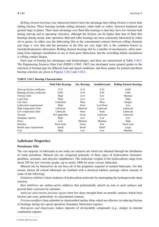
3-134 Section 3
Rolling element bearings (see subsection below) have the advantage that rolling friction is lower thansliding friction. These bearings include rolling elements, either balls or rollers, between hardened andground rings or plates. Their main advantage over ßuid Þlm bearings is that they have low friction bothduring start-up and at operating velocities, although the friction can be higher than that of ßuid Þlmbearings during steady state operation. Ball and roller bearings are most commonly lubricated by eitheroil or grease. In either case the lubricating Þlm at the concentrated contacts between rolling elementsand rings is very thin and the pressures in the Þlm are very high; this is the condition known aselastohydrodynamic lubrication. Rolling element bearings fail by a number of mechanisms, often stem-ming from improper installation or use or from poor lubrication, but the overriding failure mechanismis rolling contact fatigue.
Each type of bearing has advantages and disadvantages, and these are summarized in Table 3.10.3.The Engineering Sciences Data Unit (ESDU) (1965; 1967) has developed some general guides to theselection of bearing type for different load and speed conditions, and those guides for journal and thrustbearing selection are given in Figures 3.10.2 and 3.10.3.
Lubricant Properties
Petroleum Oils
The vast majority of lubricants in use today are mineral oils which are obtained through the distillationof crude petroleum. Mineral oils are composed primarily of three types of hydrocarbon structures:parafÞnic, aromatic, and alicyclic (naphthenic). The molecular weights of the hydrocarbons range fromabout 250 for low-viscosity grades, up to nearly 1000 for more-viscous lubricants.
Mineral oils by themselves do not have all of the properties required of modern lubricants. For thatreason, almost all current lubricants are fortiÞed with a chemical additive package which consists ofsome of the following:
Oxidation inhibitors limit oxidation of hydrocarbon molecules by interrupting the hydroperoxide chainreaction.
Rust inhibitors are surface-active additives that preferentially adsorb on iron or steel surfaces andprevent their corrosion by moisture.
Antiwear and extreme pressure agents form low shear strength Þlms on metallic surfaces which limitfriction and wear, particularly in concentrated contacts.
Friction modiÞers form adsorbed or chemisorbed surface Þlms which are effective in reducing frictionof bearings during low-speed operation (boundary lubrication regime).
Detergents and dispersants reduce deposits of oil-insoluble compounds (e.g., sludge) in internalcombustion engines.
TABLE 3.10.3 Bearing Characteristics
Fluid Film Bearings Dry Bearings Semilubricated Rolling Element Bearings
Start-up friction coefÞcient 0.25 0.15 0.10 0.002Running friction coefÞcient 0.001 0.10 0.05 0.001Velocity limit High Low Low MediumLoad limit High Low Low HighLife limit Unlimited Wear Wear FatigueLubrication requirements High None Low/None LowHigh temperature limit Lubricant Material Lubricant LubricantLow temperature limit Lubricant None None LubricantVacuum Not applicable Good Lubricant LubricantDamping capacity High Low Low LowNoise Low Medium Medium HighDirt/dust Need Seals Good Fair Need sealsRadial space requirement Small Small Small LargeCost High Low Low Medium
© 1999 by CRC Press LLC
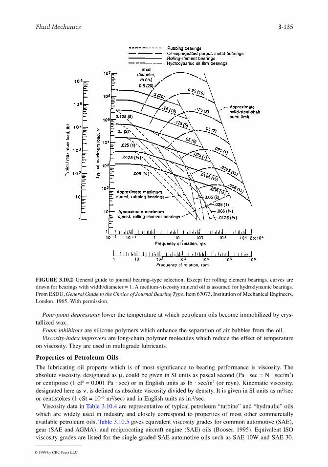
Fluid Mechanics 3-135
Pour-point depressants lower the temperature at which petroleum oils become immobilized by crys-tallized wax.
Foam inhibitors are silicone polymers which enhance the separation of air bubbles from the oil.Viscosity-index improvers are long-chain polymer molecules which reduce the effect of temperature
on viscosity. They are used in multigrade lubricants.
Properties of Petroleum Oils
The lubricating oil property which is of most signiÞcance to bearing performance is viscosity. Theabsolute viscosity, designated as m, could be given in SI units as pascal second (Pa á sec = N á sec/m2)or centipoise (1 cP = 0.001 Pa á sec) or in English units as lb á sec/in2 (or reyn). Kinematic viscosity,designated here as n, is deÞned as absolute viscosity divided by density. It is given in SI units as m2/secor centistokes (1 cSt = 10Ð6 m2/sec) and in English units as in.2/sec.
Viscosity data in Table 3.10.4 are representative of typical petroleum ÒturbineÓ and ÒhydraulicÓ oilswhich are widely used in industry and closely correspond to properties of most other commerciallyavailable petroleum oils. Table 3.10.5 gives equivalent viscosity grades for common automotive (SAE),gear (SAE and AGMA), and reciprocating aircraft engine (SAE) oils (Booser, 1995). Equivalent ISOviscosity grades are listed for the single-graded SAE automotive oils such as SAE 10W and SAE 30.
FIGURE 3.10.2 General guide to journal bearingÐtype selection. Except for rolling element bearings, curves aredrawn for bearings with width/diameter = 1. A medium-viscosity mineral oil is assumed for hydrodynamic bearings.From ESDU, General Guide to the Choice of Journal Bearing Type, Item 67073, Institution of Mechanical Engineers,London, 1965. With permission.
© 1999 by CRC Press LLC
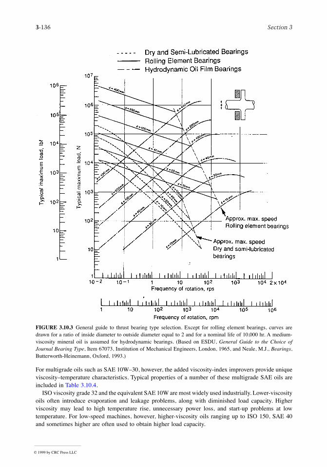
3-136 Section 3
For multigrade oils such as SAE 10WÐ30, however, the added viscosity-index improvers provide uniqueviscosityÐtemperature characteristics. Typical properties of a number of these multigrade SAE oils areincluded in Table 3.10.4.
ISO viscosity grade 32 and the equivalent SAE 10W are most widely used industrially. Lower-viscosityoils often introduce evaporation and leakage problems, along with diminished load capacity. Higherviscosity may lead to high temperature rise, unnecessary power loss, and start-up problems at lowtemperature. For low-speed machines, however, higher-viscosity oils ranging up to ISO 150, SAE 40and sometimes higher are often used to obtain higher load capacity.
FIGURE 3.10.3 General guide to thrust bearing type selection. Except for rolling element bearings, curves aredrawn for a ratio of inside diameter to outside diameter equal to 2 and for a nominal life of 10,000 hr. A medium-viscosity mineral oil is assumed for hydrodynamic bearings. (Based on ESDU, General Guide to the Choice ofJournal Bearing Type, Item 67073, Institution of Mechanical Engineers, London, 1965, and Neale, M.J., Bearings,Butterworth-Heinemann, Oxford, 1993.)
© 1999 by CRC Press LLC
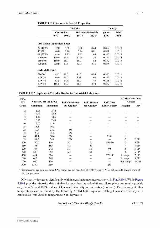
Fluid Mechanics 3-137
Oil viscosity decreases signiÞcantly with increasing temperature as shown in Fig. 3.10.4. While Figure3.10.4 provides viscosity data suitable for most bearing calculations, oil suppliers commonly provideonly the 40°C and 100°C values of kinematic viscosity in centistokes (mm2/sec). The viscosity at othertemperatures can be found by the following ASTM D341 equation relating kinematic viscosity n incentistokes (mm2/sec) to temperature T in degrees F:
(3.10.2)
TABLE 3.10.4 Representative Oil Properties
Viscosity Density
Centistokes 10-6 reyns(lbásec/in2) gm/cc lb/in3
40°C 100°C 104°F 212°F 40°C 104°F
ISO Grade (Equivalent SAE)
32 (10W) 32.0 5.36 3.98 0.64 0.857 0.031046 (20) 46.0 6.76 5.74 0.81 0.861 0.031168 (20W) 68.0 8.73 8.53 1.05 0.865 0.0313100 (30) 100.0 11.4 12.60 1.38 0.869 0.0314150 (40) 150.0 15.0 18.97 1.82 0.872 0.0315220 (50) 220.0 19.4 27.91 2.36 0.875 0.0316
SAE Multigrade
5W-30 64.2 11.0 8.15 0.99 0.860 0.031110W-30 69.0 11.0 8.81 1.08 0.865 0.031210W-40 93.5 14.3 11.9 1.45 0.865 0.031220W-50 165.5 18.7 21.3 2.74 0.872 0.0315
TABLE 3.10.5 Equivalent Viscosity Grades for Industrial Lubricants
ISO-VG
Grade
Viscosity, cSt (at 40°C) SAE CrankcaseOil Gradesa
SAE AircraftOil Gradesa
SAE GearLube Gradesa
AGMA Gear Lube Grades
Mimimum Maximum Regular EP
2 1.98 2.42 Ñ Ñ Ñ Ñ Ñ3 2.88 3.52 Ñ Ñ Ñ Ñ Ñ5 4.14 5.06 Ñ Ñ Ñ Ñ Ñ7 6.12 7.48 Ñ Ñ Ñ Ñ Ñ
10 9.00 11.0 Ñ Ñ Ñ Ñ Ñ15 13.5 16.5 Ñ Ñ Ñ Ñ Ñ22 19.8 24.2 5W Ñ Ñ Ñ Ñ32 28.8 35.2 10W Ñ Ñ Ñ Ñ46 41.4 50.6 15W Ñ 75W 168 61.2 74.8 20W Ñ Ñ 2 2 EP
100 90.0 110 30 65 80W-90 3 3 EP150 135 165 40 80 Ñ 4 4 EP220 198 242 50 100 90 5 5 EP320 288 352 60 120 Ñ 6 6 EP460 414 506 Ñ Ñ 85W-140 7 comp 7 EP680 612 748 Ñ Ñ Ñ 8 comp 8 EP
1000 900 1100 Ñ Ñ Ñ 8A comp 8A EP1500 1350 1650 Ñ Ñ 250 Ñ Ñ
a Comparisons are nominal since SAE grades are not speciÞed at 40°C viscosity; VI of lubes could change some of the comparisons.
loglog . logn +( ) = - +( )0 7 460A B T
© 1999 by CRC Press LLC
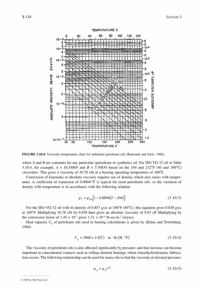
3-138 Section 3
where A and B are constants for any particular (petroleum or synthetic) oil. For ISO VG-32 oil in Table3.10.4, for example, A = 10.54805 and B = 3.76834 based on the 104 and 212°F (40 and 100°C)viscosities. This gives a viscosity of 10.78 cSt at a bearing operating temperature of 160°F.
Conversion of kinematic to absolute viscosity requires use of density, which also varies with temper-ature. A coefÞcient of expansion of 0.0004/°F is typical for most petroleum oils, so the variation ofdensity with temperature is in accordance with the following relation:
(3.10.3)
For the ISO-VG-32 oil with its density of 0.857 g/cc at 100°F (40°C), this equation gives 0.838 g/ccat 160°F. Multiplying 10.78 cSt by 0.838 then gives an absolute viscosity of 9.03 cP. Multiplying bythe conversion factor of 1.45 ´ 10Ð7 gives 1.31 ´ 10Ð6 lbásec/in.2 (reyns).
Heat capacity Cp of petroleum oils used in bearing calculations is given by (Klaus and Tewksburg,1984)
(3.10.4)
The viscosity of petroleum oils is also affected signiÞcantly by pressure, and that increase can becomeimportant in concentrated contacts such as rolling element bearings where elastohydrodynamic lubrica-tion occurs. The following relationship can be used for many oils to Þnd the viscosity at elevated pressure:
(3.10.5)
FIGURE 3.10.4 ViscosityÐtemperature chart for industrial petroleum oils (Ramondi and Szeri, 1984).
r rT T= - -( )[ ]104 1 0 0004 104.
C Tp = + ( ) × × °( )3860 4 5. in. lb lb F
m m ap o
pe=
© 1999 by CRC Press LLC
Fluid Mechanics 3-139
where mo is the viscosity at atmospheric pressure, mp is the viscosity at pressure p, and a is thepressureÐviscosity exponent. The pressureÐviscosity exponent can be obtained from lubricant suppliers.
Synthetic Oils
Synthetic oils of widely varying characteristics are Þnding increasing use for applications at extremetemperatures and for their unique physical and chemical characteristics. Table 3.10.6 gives a fewrepresentative examples of synthetic oils which are commercially available. Cost of the synthetics,ranging up to many times that of equivalent petroleum oils, is a common deterrent to their use wherepetroleum products give satisfactory performance
Greases
Grease is essentially a suspension of oil in a thickening agent, along with appropriate additives. The oilgenerally makes up between 75 and 90% of the weight of a grease, and it is held in place by the gelstructure of the thickener to carry out its lubricating function. The simplicity of the lubricant supplysystem, ease of sealing, and corrosion protection make grease the Þrst choice for many ball-and-rollerbearings, small gear drives, and slow-speed sliding applications (Booser, 1995). Consistencies of greasesvary from soap-thickened oils that are ßuid at room temperature to hard brick-types that may be cutwith a knife. Greases of NLGI Grade 2 stiffness (ASTM D217) are most common. Softer greases downto grade 000 provide easier feeding to multiple-row roller bearings and gear mechanisms. Stiffer Grade3 is used in some prepacked ball bearings to avoid mechanical churning as the seals hold the grease inclose proximity with the rotating balls.
TABLE 3.10.6 Properties of Representative Synthetic Oils
Pour Point,
°C
Flash Point,
°C
Viscosity, cSt at
Type 100°C 40°C Ð54°C Typical Uses
Synthetic hydrocarbonsMobil 1, 5W-30a 11 58 Ñ Ð54 221 Auto enginesSHC 824a 6.0 32 Ñ Ð54 249 Gas turbinesSHC 629a 19 141 Ñ Ð54 238 Gears
Organic estersMIL-L-7808 3.2 13 12,700 Ð62 232 Jet enginesMIL-L-23699 5.0 24 65,000 Ð56 260 Jet enginesSynesstic 68b 7.5 65 Ñ Ð34 266 Air compressors, hydraulics
PolyglycolsLB-300-Xc 11 60 Ñ Ð40 254 Rubber seals50-HB-2000c 70 398 Ñ Ð32 226 Water solubility
PhosphatesFyrquel 150d
Fyrquel 220d
4.35.0
2944
ÑÑ
Ð24Ð18
236236
Fire-resistant ßuids for die casting, air compressors and hydraulic systems
SiliconesSF-96 (50) 16 37 460 Ð54 316 Hydraulic and damping ßuids
Hydraulic and damping ßuidsSF-95 (1000) 270 650 7,000 Ð48 316F-50 16 49 2,500 Ð74 288 Aircraft and missiles
FluorochemicalsHalocarbon 27e 3.7 30 Ñ Ð18 None Oxygen compressors, liquid-oxygen
systemsKrytox 103f 5.2 30 Ñ Ð45 None
a Mobil Oil Corp.b Exxon Corp.c Union Carbide Chemials Co.d Akzo Chemicalse Halocarbon Products Corp.f DuPont Co.
© 1999 by CRC Press LLC
3-140 Section 3
Petroleum oils are used in most greases; the oils generally are in the SAE 30 range, with a viscosityof about 100 to 130 cSt at 40°C. Lower-viscosity oil grades are used for some high-speed applicationsand for temperatures below about Ð20°C. Higher-viscosity oils are used in greases for high loads andlow speeds. Synthetic oils are used only when their higher cost is justiÞed by the need for specialproperties, such as capability for operation below Ð20°C or above 125 to 150°C.
The most common gelling agents are the fatty acid metallic soaps of lithium, calcium, sodium, oraluminum in concentrations of 8 to 25%. Of these, the most popular is lithium 12-hydroxystearate;greases based on this lithium thickener are suitable for use at temperatures up to 110°C, where somelithium soaps undergo a phase change. Greases based on calcium or aluminum soaps generally have anupper temperature limit of 65 to 80°C, but this limit can be signiÞcantly raised to the 120 to 125°Crange through new complex soap formulations. Calcium-complex soaps with improved high-temperaturestability, for instance, are prepared by reacting both a high-molecular-weight fatty acid (e.g., stearicacid) and a low-molecular-weight fatty acid (acetic acid) with calcium hydroxide dispersed in mineral oil.
Inorganic thickeners, such as Þne particles of bentonite clay, are inexpensively applied by simplemixing with oil to provide nonmelting greases for use up to about 140°C. Polyurea nonmelting organicpowders are used in premium petroleum greases for applications up to about 150 to 170°C.
Additives, such as those mentioned in the subsection on petroleum oils, are added to grease to improveoxidation resistance, rust protection, or extreme pressure properties. Because of the incompatibility ofoils, thickeners, and additives, greases of different types should be mixed only with caution.
Solid Lubricants
Solid lubricants provide thin solid Þlms on sliding or rolling/sliding surfaces to reduce friction and wear.They are particularly useful for applications involving high operating temperatures, vacuum, nuclearradiation, or other environments which limit the use of oils or greases. Solid lubricant Þlms do notprevent moving surfaces from contacting each other, so they cannot eliminate wear and their lives arelimited by wear. The properties of some of the most common solid lubricants are given in Table 3.10.7.
The most important inorganic solid lubricants are layerÐlattice solids such as molybdenum disulÞde(MoS2) and graphite. These materials are characterized by strong covalent or ionic bonding betweenatoms in individual layers, but relatively weak van der Waals bonds between layers, enabling the layers
TABLE 3.10.7 Properties of Selected Solid Lubricants
Acceptable Usage Temperature, °C Average Friction CoefÞcient, fMinimum Maximum
Material In AirIn N2 or Vacuum In Air
In N2 orVacuum In Air
In N2 orVacuum Remarks
Molybdenum disulÞde,MoS2
Ð240 Ð240 370 820 0.10Ð0.25 0.05Ð0.10 Low f, carries high load, good overall lubricant, can promote metal corrosion
Graphite Ð240 Ñ 540 Unstable in
vacuum
0.10Ð0.30 0.02Ð0.45 Low f and high load capacity in air, high f and wear in vacuum, conducts electricity
PTFE Ð70 Ð70 290 290 0.02Ð0.15 0.02Ð0.15 Lowest f of solid lubricants, load capacity moderate and decreases at elevated temperature
Calcium ßourideÐbarium ßuoride eutectic, CaF2ÐBaF2
430 430 820 820 0.10Ð0.25 above 540°C
0.25Ð0.40 below 540°C
Same as in air
Can be used at higher temperature than other solid lubricants, high f below 540°C
ModiÞed from Booser, E.R., in Encyclopedia of Chemical Technology, 4th ed., Vol. 15, John Wiley & Sons, New York, 1995, 463Ð517.
© 1999 by CRC Press LLC
Fluid Mechanics 3-141
to slide easily relative to one another. Graphite is a very effective lubricant Þlm when moisture or watervapor is present, since adsorbed water vapor lubricates the sliding layers, but it has poor friction propertiesin vacuum or other low-humidity applications. Molybdenum disulÞde does not require the presence ofadsorbed water vapor, so it is widely used in vacuum or space applications.
The most commonly used organic solid lubricant is polytetraßuoroethylene (PTFE) which can beused either as a fused surface coating or as a self-lubricating material (see subsection on plastics). Itslow friction is attributed to the smooth proÞle of the PTFE molecule. The chemical inertness of PTFEmakes it attractive for chemical and food-processing applications.
New ceramic-based solid lubricants have been developed for high-temperature applications, such asheat engines or space uses. One of the most promising of these is a calcium ßuorideÐbarium ßuorideeutectic, which can be used at temperatures exceeding 800°C.
Fluid Film Bearings
Journal Bearings
A journal bearing consists of an approximately cylindrical bearing body or sleeve around a rotatingcylindrical shaft. In general, journal bearings are found in motors, pumps, generators, appliances, andinternal combustion engines in which a ßuid lubricant is used; and in smaller mechanisms such asswitches, clocks, small motors, and circuit breakers in which a solid lubricant such as graphite, grease,or certain plastics serves to reduce friction. Air (gas) bearings are designed to utilize both ßuid mechanicsprinciples when operating and solid lubricantÐsurfaced materials for start, stop, and emergency opera-tions.
A hydrodynamic journal bearing maintains separation of shaft from bearing because the lubricantviscosity and the speed of the shaft create pressure in the converging portion of the ßuid Þlm whichcarries load. The governing equations were Þrst developed by Reynolds (1886). Their solution has ledto numerous computer solutions, including those used for this section.
Journal Bearing Design. Figure 3.10.5 shows schematics of frequently used types of journal bearing inwhich one or more lobes of cylindrical shape are positioned around the shaft, their axis being assumedparallel to the shaft axis. The features of each design and applications where it is often found are listedin Table 3.10.8.
Noncontact journal bearings are designed to assure a continuous supply of lubricant to the load-carrying section, and the bearing grooves in Figure 3.10.5 are designed for that purpose. Oil must beresupplied to the bearing because of the continuous loss of lubricant as it is forced from the bearing bythe load-carrying pressures generated within it. The subsection on lubricant supply methods describessome of the many systems designed to assure this supply and to cool the lubricant at the same time.
Controlling Variables. DeÞnitions of the variables involved in journal bearing analysis are containedin Table 3.10.9. Because of the large range of many variables, nondimensional quantities are often usedwhich are independent of the dimensional unit system involved. Examples are given in the Englishsystem unless otherwise stated.
Calculating Bearing Performance. Journal bearing performance can be calculated directly from dedicatedcomputer codes which take account of load, speed, oil type, and delivery system, as well as bearingdimensions. This subsection presents two approximate solutions: a simple thermal approach and a setof interpolation tables based on computer solutions.
Thermal Approach. It is assumed that the bearing is operating at a constant but elevated temperature.A predicted operating temperature can then be found as a function of an assumed viscosity. A solutionis found when the assumed viscosity equals the lubricant viscosity at that temperature. Three equationsare used for this method. For radial loads, the power dissipation is
(3.10.6)H j N D L Cp = ( ) ×p m3 2 360 in. lb sec
© 1999 by CRC Press LLC
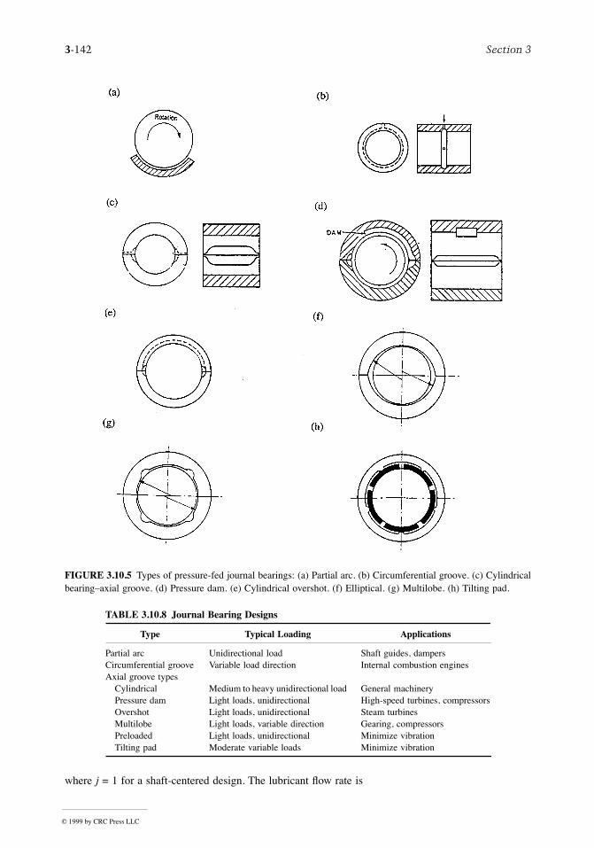
3-142 Section 3
where j = 1 for a shaft-centered design. The lubricant ßow rate is
FIGURE 3.10.5 Types of pressure-fed journal bearings: (a) Partial arc. (b) Circumferential groove. (c) CylindricalbearingÐaxial groove. (d) Pressure dam. (e) Cylindrical overshot. (f) Elliptical. (g) Multilobe. (h) Tilting pad.
TABLE 3.10.8 Journal Bearing Designs
Type Typical Loading Applications
Partial arc Unidirectional load Shaft guides, dampersCircumferential groove Variable load direction Internal combustion enginesAxial groove types
Cylindrical Medium to heavy unidirectional load General machineryPressure dam Light loads, unidirectional High-speed turbines, compressorsOvershot Light loads, unidirectional Steam turbinesMultilobe Light loads, variable direction Gearing, compressorsPreloaded Light loads, unidirectional Minimize vibrationTilting pad Moderate variable loads Minimize vibration
© 1999 by CRC Press LLC
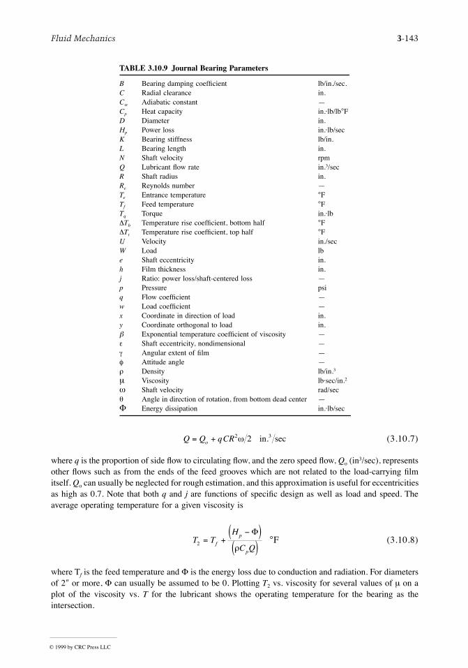
Fluid Mechanics 3-143
(3.10.7)
where q is the proportion of side ßow to circulating ßow, and the zero speed ßow, Qo (in3/sec), representsother ßows such as from the ends of the feed grooves which are not related to the load-carrying Þlmitself. Qo can usually be neglected for rough estimation, and this approximation is useful for eccentricitiesas high as 0.7. Note that both q and j are functions of speciÞc design as well as load and speed. Theaverage operating temperature for a given viscosity is
°F (3.10.8)
where Tf is the feed temperature and F is the energy loss due to conduction and radiation. For diametersof 2² or more, F can usually be assumed to be 0. Plotting T2 vs. viscosity for several values of m on aplot of the viscosity vs. T for the lubricant shows the operating temperature for the bearing as theintersection.
TABLE 3.10.9 Journal Bearing Parameters
B Bearing damping coefÞcient lb/in./sec.C Radial clearance in.Ca Adiabatic constant ÑCp Heat capacity in.álb/lb°FD Diameter in.Hp Power loss in.álb/secK Bearing stiffness lb/in.L Bearing length in.N Shaft velocity rpmQ Lubricant ßow rate in.3/secR Shaft radius in.Re Reynolds number ÑTe Entrance temperature °FTf Feed temperature °FTq Torque in.álbDTb Temperature rise coefÞcient, bottom half °FDTt Temperature rise coefÞcient, top half °FU Velocity in./secW Load lbe Shaft eccentricity in.h Film thickness in.j Ratio: power loss/shaft-centered loss Ñp Pressure psiq Flow coefÞcient Ñw Load coefÞcient Ñx Coordinate in direction of load in.y Coordinate orthogonal to load in.b Exponential temperature coefÞcient of viscosity Ñe Shaft eccentricity, nondimensional Ñg Angular extent of Þlm Ñf Attitude angle Ñr Density lb/in.3
m Viscosity lbásec/in.2
w Shaft velocity rad/secq Angle in direction of rotation, from bottom dead center ÑF Energy dissipation in.álb/sec
Q Q qCRo= + 2 32w in. sec
T TH
C Qf
p
p
2 = +-( )
( )F
r
© 1999 by CRC Press LLC
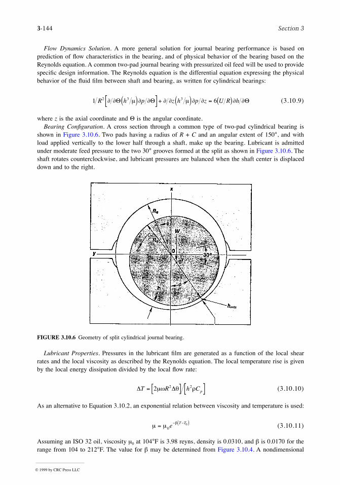
3-144 Section 3
Flow Dynamics Solution. A more general solution for journal bearing performance is based onprediction of ßow characteristics in the bearing, and of physical behavior of the bearing based on theReynolds equation. A common two-pad journal bearing with pressurized oil feed will be used to providespeciÞc design information. The Reynolds equation is the differential equation expressing the physicalbehavior of the ßuid Þlm between shaft and bearing, as written for cylindrical bearings:
(3.10.9)
where z is the axial coordinate and Q is the angular coordinate.Bearing ConÞguration. A cross section through a common type of two-pad cylindrical bearing is
shown in Figure 3.10.6. Two pads having a radius of R + C and an angular extent of 150°, and withload applied vertically to the lower half through a shaft, make up the bearing. Lubricant is admittedunder moderate feed pressure to the two 30° grooves formed at the split as shown in Figure 3.10.6. Theshaft rotates counterclockwise, and lubricant pressures are balanced when the shaft center is displaceddown and to the right.
Lubricant Properties. Pressures in the lubricant Þlm are generated as a function of the local shearrates and the local viscosity as described by the Reynolds equation. The local temperature rise is givenby the local energy dissipation divided by the local ßow rate:
(3.10.10)
As an alternative to Equation 3.10.2, an exponential relation between viscosity and temperature is used:
(3.10.11)
Assuming an ISO 32 oil, viscosity m0 at 104°F is 3.98 reyns, density is 0.0310, and b is 0.0170 for therange from 104 to 212°F. The value for b may be determined from Figure 3.10.4. A nondimensional
FIGURE 3.10.6 Geometry of split cylindrical journal bearing.
1 62 3 3R h p z h p z U R h¶ ¶ m ¶ ¶ ¶ ¶ m ¶ ¶ ¶ ¶Q Q Q( )[ ] + ( ) = ( )
D DT R h Cp= [ ] [ ]2 2 2mw q r
m m b= - -( )0
0eT T
© 1999 by CRC Press LLC
Fluid Mechanics 3-145
coefÞcient, Ca, the adiabatic coefÞcient, is used as an indicator of the severity of thermal heating in adesign. It contains the several factors responsible for temperature rise.
(3.10.12)
Bearing Performance Tables. Using computer-generated solutions of the Reynolds equation for thepressure Þeld over the bearing surface, the relevant performance properties of the bearing/lubricantsystem can be determined. A number of programs are commercially available for this purpose. In orderto illustrate how the behavior of a journal bearing can be determined, a two-pad split cylindrical bearingwith an L/D of 0.5 has been selected, and a proprietary computer code has been used to develop a groupof performance quantities for such a bearing. The code accounts for the internal lubricant circulation,including mixing in the inlet groove of feed lubricant with warm lubricant from the upper half, resultingin the viscosity mf . The primary characteristics of the bearing are load, stiffness, and damping. Each ofthese factors is presented in nondimensional terms in Table 3.10.10, and the corresponding dimensionaland other quantities are given as follows:
The axial length/diameter ratio also inßuences the performance of a journal bearing. To illustrate this,Table 3.10.11 presents the performance of longer bearings (L/D = 0.75 and 1.00) for comparison to themore common L/D = 0.5 results in Table 3.10.10.
Comparing Tables 3.10.10 and 3.10.11, the use of longer bearings has several important effects onoperation and performance. Comparing key variables, the effects at an eccentricity of ratio of 0.7 are asfollows:
Effect of Turbulence. Turbulence is a mixing phenomenon that occurs in larger high-speed bearings.When this behavior occurs, the simple viscous drag behavior that has been assumed in the preceding
Variable L/D = 0.5 L/D = 0.75 L/D = 1.00
Load, w 0.28 0.69 1.21Flow, q 0.69 0.82 0.88Attitude angle, f 36.4 36.1 35.8Power ratio, j 1.00 1.15 1.17Stiffness, Kxx 1.38 3.06 5.03Damping, Bxx 0.99 2.52 4.31
C R C Cf pa m bw r= ( )22
Film thickness, in. = 3.10.13a)h C e1 +( )cos (Q
Shaft eccentricity, in. = 3.10.13b)e Ce (
Load, lb 3.10.13c)W w R C DL= ( )[ ]62
mw (
Flow, in.3 3.10.13d)sec (Q q CR= ( )2 2w
Power loss, in. lb 3.10.13e)× = ( )sec (H j R L Cp 2 2 3pmw
Stiffness, lb in. 3.10.13f)S K R R Cxx xx= ( )62
mw (
Damping, lb sec in. 3.10.13g)× = ( )D B R R Cxx xx12 3m . (
© 1999 by CRC Press LLC
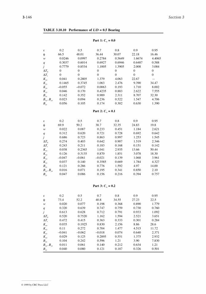
3-146 Section 3
TABLE 3.10.10 Performance of L/D = 0.5 Bearing
Part 1: Ca = 0.0
e 0.2 0.5 0.7 0.8 0.9 0.95f 66.5 48.01 36.44 30.07 22.18 16.46w 0.0246 0.0997 0.2784 0.5649 1.6674 4.4065q 0.3037 0.6014 0.6927 0.6946 0.6487 0.588j 0.7779 0.8534 1.1005 1.3905 2.008 3.084DTb 0 0 0 0 0 0DTt 0 0 0 0 0 0Kxx 0.041 0.2805 1.379 4.063 22.67 ÑKxy 0.1465 0.3745 1.063 2.476 9.390 34.47Kyx Ð0.055 Ð0.072 0.0063 0.193 1.710 8.002Kyy 0.046 0.170 0.4235 0.883 2.622 7.555Bxx 0.142 0.352 0.989 2.311 8.707 32.30Bxy, Byx 0.023 0.094 0.236 0.522 1.547 4.706Byy 0.056 0.105 0.174 0.302 0.630 1.390
Part 2: Ca = 0.1
e 0.2 0.5 0.7 0.8 0.9 0.95f 69.9 50.2 38.7 32.35 24.83 19.8w 0.022 0.087 0.233 0.451 1.184 2.621q 0.312 0.620 0.721 0.728 0.692 0.642j 0.686 0.723 0.863 0.997 1.253 1.545DTb 0.274 0.403 0.642 0.907 1.519 2.346DTt 0.243 0.211 0.183 0.168 0.151 0.142Kxx 0.038 0.2365 1.041 2.935 13.66 50.44Kxy 0.126 0.3135 0.870 1.851 3.078 18.30Kyx Ð0.047 Ð0.061 Ð0.021 0.139 1.068 3.961Kyy 0.037 0.140 0.3585 0.669 1.784 4.327Bxx 0.121 0.286 0.776 1.592 4.97 14.00Bxy, Byx 0.016 0.071 0.195 0.341 0.850 2.10Byy 0.047 0.086 0.156 0.216 0.394 0.757
Part 3: Ca = 0.2
e 0.2 0.5 0.7 0.8 0.9 0.95f 73.4 52.2 40.8 34.55 27.23 22.5w 0.020 0.077 0.198 0.368 0.890 1.779q 0.320 0.639 0.747 0.759 0.730 0.760j 0.613 0.628 0.712 0.791 0.933 1.092DTb 0.520 0.7520 1.162 1.594 2.521 3.651DTt 0.472 0.415 0.363 0.333 0.301 0.284Kxx 0.035 0.1925 0.830 2.156 8.86 28.6Kxy 0.11 0.272 0.704 1.477 4.515 11.72Kyx Ð0.041 Ð0.062 Ð0.018 0.074 0.640 2.371Kyy 0.029 0.125 0.2895 0.551 1.375 2.932Bxx 0.104 0.242 0.596 1.21 3.90 7.830Bxy, Byx 0.011 0.061 0.140 0.212 0.634 1.21Byy 0.040 0.080 0.121 0.187 0.326 0.501
© 1999 by CRC Press LLC
Fluid Mechanics 3-147
Part 4 Ca = 0.4
e 0.2 0.5 0.7 0.8 0.9 0.95f 80.2 56.0 44.5 38.4 31.3 26.7w 0.016 0.061 0.148 0.260 0.562 1.000q 0.331 0.6720 0.795 0.815 0.797 0.760j 0.504 0.498 0.534 0.570 0.637 0.716DTb 0.946 1.33 1.97 2.61 3.87 5.26DTt 0.898 0.801 0.712 0.658 0.597 0.562Kxx 0.029 0.137 0.538 1.295 4.56 12.6Kxy 0.085 0.206 0.503 0.985 2.67 6.17Kyx Ð0.0315 Ð0.0548 0.0298 0.0233 0.321 1.136Kyy 0.019 0.094 0.214 0.382 0.860 1.68Bxx 0.079 0.175 0.397 0.734 1.75 3.44Bxy, Byx 0.0041 0.042 0.094 0.166 0.329 0.55Byy 0.030 0.064 0.092 0.131 0.120 0.276
TABLE 3.10.11 Performance of Long Bearings
Part 1: L/D = 0.75, Ca = 0.0
e 0.2 0.5 0.7 0.8 0.9 0.95f 64.74 46.54 36.13 30.17 22.64 17.03w 0.0705 0.2714 0.6947 1.311 3.440 8.241q 0.392 0.738 0.825 0.811 0.737 0.6545j 0.777 0.871 1.145 1.450 2.184 3.233DTb 0 0 0 0 0 0DTt 0 0 0 0 0 0Kxx 0.121 0.706 3.065 8.506 41.5 ÑKxy 0.418 0.992 2.517 5.228 18.1 59.0Kyx Ð0.123 Ð0.189 0.052 0.404 3.18 16.2Kyy 0.113 0.429 1.012 1.891 5.33 13.49Bxx 0.423 0.982 2.52 5.16 17.7 54.4Bxy, Byx 0.057 0.249 0.609 1.10 3.24 7.58Byy 0.127 0.263 0.444 0.641 1.35 2.32
Part 2: L/D = 1.00, Ca = 0.00
e 0.2 0.5 0.7 0.8 0.9 0.95f 63.2 45.3 35.8 30.3 22.9 17.4w 0.138 0.506 1.214 2.18 5.34 12.15q 0.444 0.800 0.879 0.856 0.769 0.679j 0.782 0.886 1.174 1.768 2.250 3.323DTb 0 0 0 0 0 0DTt 0 0 0 0 0 0Kxx 0.234 1.254 5.026 13.24 60.9 ÑKxy 0.818 1.795 4.142 8.12 26.8 83.5Kyx Ð0.201 Ð0.313 Ð0.075 0.671 4.96 24.9Kyy 0.198 0.732 1.64 2.95 8.04 19.5Bxx 0.82 1.87 4.31 8.27 26.5 75.9Bxy, Byx 0.10 0.45 0.97 1.68 4.78 10.36Byy 0.21 0.46 0.70 0.98 2.02 3.24
TABLE 3.10.10 (continued) Performance of L/D = 0.5 Bearing
© 1999 by CRC Press LLC
3-148 Section 3
subsections is broken up by numerous eddies which increase the drag. The Reynolds number is anondimensional quantity that expresses this factor:
(3.10.14)
where h is the local Þlm thickness, U is the relative velocity of one surface with respect to the other, ris the ßuid density, and m is the local viscosity.
The inßuence of turbulence on an L/D = 0.5 bearing is shown in Table 3.10.12. Examination of Table3.10.12 shows that the principal effects of operation in the turbulent regime with a Reynolds numberabove about 1000 are in the greater power required ( j) and the maximum bearing temperature. Loadcapacity and ßow are only moderately affected.
Example Calculation. The problem is to design a two-pad cylindrical bearing for support of a rotorhaving a bearing load of 8000 lb, a shaft diameter of 6 in., and a speed of 3600 rpm. Assume use ofISO VG-32 oil fed at a temperature of 120°F. Compute operating characteristics for a 3-in.-long bearing.Assume a radial clearance of 0.0044 in.
Feed viscosity, mf = 3.98 ´ 10Ð6 e Ð0.00170(120Ð104) = 3.03 ´ 10Ð6 reyn
Angular velocity, w = 3600 ´ 2p/60 = 377 rad/secAdiabatic coefÞcient: Ca = 2 ´ 3.03 ´ 10Ð6 ´ 0.0170 ´ 377 ´ (3/0.0044)2/0.0310/4320 = 0.1345Load coefÞcient (from Equation 3.10.13c: w = 8000/[6 ´ 3.03 ´ 10Ð6 ´ 377 ´ 3 ´ 6 ´ (33/0.0044)2]
= 0.139
The desired solution lies between Part 2 and Part 3 of Table 3.10.10. By using linear interpolationbetween the tabulated values for Ca of 0.1 and 0.2, and values of e of 0.7 and 0.8, an approximateoperating point of Ca = 0.1345 yields the following coefÞcients: e = 0.729, w = 0.279, q = 0.733, j =0.860, and DTb = 0.915.
By using Equations 3.10.13, the dimensional operating results are:
Shaft velocity: w = 3600 ´ 2p/60 = 377 rad/secFlow: Q = 0.733 ´ 0.0044 ´ 32 ´ 377 = 5.47 in3/secPower loss: Hp = 0.860 ´ 2p ´ 3.03 ´ 10Ð6 ´ 3772 ´ 33 ´ 3/0.0044 = 42.8 in.álb/secOil temperature: Tb = 120 + 0.915/0.0170 = 174°F
Thrust Bearings
Types of Thrust Bearings. Oil Þlm thrust bearings range from coin-size ßat washers to sophisticatedassemblies many feet in diameter. Of the six common types of thrust bearings shown in Table 3.10.13,the Þrst Þve are hydrodynamic. As with journal bearings, each of these generates oil Þlm pressure when
TABLE 3.10.12. Inßuence of Turbulence (e = 0.7, Ca = 0.2, arc = 150°)
Re 0 1000 2000 4000
f 40.8 43.8 46.4 49.2w 0.198 0.171 0.197 0.221q 0.747 0.809 0.862 0.914j 0.712 0.983 1.459 2.124DTb 1.162 0.585 0.918 1.404Kxx 0.830 0.627 0.634 0.647Kxy 0.704 0.575 0.577 0.645Kyx Ð0.018 Ð0.034 Ð0.047 Ð0.078Kyy 0.289 0.257 0.282 0.330Bxx 0.596 0.483 0.513 0.534Bxy, Byx 0.140 0.125 0.132 0.136Byy 0.121 Ñ Ñ 0.104
R hUe = r m
© 1999 by CRC Press LLC
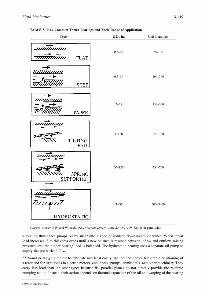
Fluid Mechanics 3-149
a rotating thrust face pumps oil by shear into a zone of reduced downstream clearance. When thrustload increases, Þlm thickness drops until a new balance is reached between inßow and outßow, raisingpressure until the higher bearing load is balanced. The hydrostatic bearing uses a separate oil pump tosupply the pressurized ßow.
Flat-land bearings, simplest to fabricate and least costly, are the Þrst choice for simple positioning ofa rotor and for light loads in electric motors, appliances, pumps, crankshafts, and other machinery. Theycarry less load than the other types because ßat parallel planes do not directly provide the requiredpumping action. Instead, their action depends on thermal expansion of the oil and warping of the bearing
TABLE 3.10.13 Common Thrust Bearings and Their Range of Application
Type O.D., in. Unit Load, psi
0.5Ð20 20Ð100
0.5Ð10 100Ð300
2Ð35 150Ð300
4Ð120 250Ð700
50Ð120 350Ð700
3Ð50 500Ð3000
Source: Booser, E.R. and Wilcock, D.F., Machine Design, June 20, 1991, 69Ð72. With permission.
© 1999 by CRC Press LLC
3-150 Section 3
material induced by heating from the passing oil Þlm. The resulting slight oil wedge then gives a loadrating of about 10 to 20% of that for the other types.
Step bearings also offer relatively simple design. With a coined or etched step, they lend themselves tomass production as small-size bearings and thrust washers. Step height for optimum load capacityapproximately equals the minimum Þlm thickness, often 0.001 in. or less. Circumferential length beyondthe step is ideally 45% of the total bearing segment (Wilcock and Booser, 1956). Step thrust bearingsare well suited for low-viscosity ßuids such as water, gasoline, fuels, and solvents. Minimum Þlmthickness in these applications is so small that features such as pivots and tapers are usually impractical.Step height must be small enough for good load capacity, yet large enough to accommodate some wearwithout becoming worn away. Step erosion by contaminants is sometimes a problem.
Tapered-land bearings provide reliable, compact designs for mid- to large-size high-speed machinessuch as turbines, compressors, and pumps. Taper height normally should be about one to three timesthe minimum Þlm thickness. For greater load capacity and to minimize wear during starting, stopping,and at low speeds, a ßat land is commonly machined at the trailing edge to occupy from 10 to 30% ofthe circumferential length of each segment. Because operation of these bearings is sensitive to load,speed, and lubricant viscosity, they are typically designed for the rated range of operating conditionsfor speciÞc machines.
Tilting-pad thrust bearings are used increasingly in turbines, compressors, pumps, and marine drives inmuch the same range of applications as tapered-land designs. They usually have a central supportingpivot for each of their three to ten bearing segments. Each of these thrust pad segments is free to adjustits position to form a nearly optimum oil wedge for widely varying loads, speeds, and lubricants, andwith rotation in both directions. A secondary leveling linkage system is commonly introduced to supportthe individual pads; this provides a further advantage over tapered-land designs by accommodating somemisalignment. Off-the-shelf units are available to match rotor shaft diameters from about 2 to 12 in.,and custom designs range up to 120 to 170 in. in outside diameter. Recent trends to increase load capacityhave led to offsetting pivots from the circumferential midpoint of a pad to about 60% beyond the leadingedge, to substituting copper for steel as the backing for a tin babbitt bearing surface, and to nonßoodedlubrication to minimize parasitic power loss from useless churning of oil passing through the bearinghousing.
Springs or other ßexible supports for thrust segments are employed for bearings ranging up to 10 ft ormore in outside diameter and carrying millions of pounds of thrust. This ßexible mounting avoids thehigh load concentration encountered by pivots in supporting large tilting-pads. Rubber backing canprovide this ßexible mounting for smaller thrust pads.
Hydrostatic thrust bearings are used where sufÞcient load support cannot be generated by oil Þlm actionwithin the bearing itself. This may be the case with low-viscosity ßuids, or for load support on an oilÞlm at standstill and very low speeds. The ßuid is Þrst pressurized by an external pump and thenintroduced into pockets in the bearing surface to ßoat the load. A compact hydrostatic thrust bearingcan sometimes be constructed with a single pocket at the end of a rotor. Larger bearings usually usethree or more pressurized pockets to resist misalignment or to support off-center loads. Hydraulic ßowresistance in the supply line to each pocket, or constant ßow to each pocket (as with ganged gear pumps)then provides any asymmetric pressure distribution needed to support an off-center load. Bearing unitload is commonly limited to about 0.5 (0.75 with Þxed ßow systems) times the hydrostatic ßuid supplypressureÑup to 5000 psi with conventional lubricating oils.
Design Factors for Thrust Bearings. In preliminary sizing, the inside diameter d of a thrust bearing ismade sufÞciently larger than the shaft to allow for assembly, and to provide for any required oil ßowto the thrust bearing inside diameter (see Figure 3.10.7). This clearance typically ranges from about 1/8
in. for a 2-in. shaft to 1/2 in. for a 10-in. shaft. Bearing outside diameter D is then set to provide bearing
© 1999 by CRC Press LLC
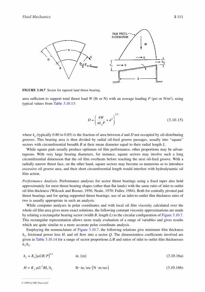
Fluid Mechanics 3-151
area sufÞcient to support total thrust load W (lb or N) with an average loading P (psi or N/m2), usingtypical values from Table 3.10.13:
(3.10.15)
where kg (typically 0.80 to 0.85) is the fraction of area between d and D not occupied by oil-distributinggrooves. This bearing area is then divided by radial oil-feed groove passages, usually into ÒsquareÓsectors with circumferential breadth B at their mean diameter equal to their radial length L.
While square pads usually produce optimum oil Þlm performance, other proportions may be advan-tageous. With very large bearing diameters, for instance, square sectors may involve such a longcircumferential dimension that the oil Þlm overheats before reaching the next oil-feed groove. With aradially narrow thrust face, on the other hand, square sectors may become so numerous as to introduceexcessive oil groove area, and their short circumferential length would interfere with hydrodynamic oilÞlm action.
Performance Analysis. Performance analyses for sector thrust bearings using a Þxed taper also holdapproximately for most thrust bearing shapes (other than ßat lands) with the same ratio of inlet to outletoil Þlm thickness (Wilcock and Booser, 1956; Neale, 1970; Fuller, 1984). Both for centrally pivoted padthrust bearings and for spring-supported thrust bearings, use of an inlet-to-outlet Þlm thickness ratio oftwo is usually appropriate in such an analysis.
While computer analyses in polar coordinates and with local oil Þlm viscosity calculated over thewhole oil Þlm area gives more-exact solutions, the following constant viscosity approximations are madeby relating a rectangular bearing sector (width B, length L) to the circular conÞguration of Figure 3.10.7.This rectangular representation allows more ready evaluation of a range of variables and gives resultswhich are quite similar to a more accurate polar coordinate analysis.
Employing the nomenclature of Figure 3.10.7, the following relations give minimum Þlm thicknessh2, frictional power loss H, and oil ßow into a sector Q. The dimensionless coefÞcients involved aregiven in Table 3.10.14 for a range of sector proportions L/B and ratios of inlet to outlet Þlm thicknessesh1/h2.
FIGURE 3.10.7 Sector for tapered land thrust bearing.
DW
k Pd
g
= +æ
èç
ö
ø÷
4 2
0 5
p
.
h K UB Ph2
0 5= ( ) ( )m
. (in. m 3.10.16a)
H K U BL hf= × ×( )m 22 lb in sec N m sec 3.10.16b). (
© 1999 by CRC Press LLC
3-152 Section 3
where B = circumferential breadth of sector at mean radius, in. (m)
Kh,Kf , Kq = dimensionless coefÞcients
L = radial length of sector, in. (m)
P = unit loading on projected area of sector, W/BL, lb/in.2 (N/m2)
U = surface velocity at mean diameter of sector, in./sec (m/sec)
W = load on a sector, lb (N)
Cp = oil speciÞc heat, in.álb/(lbá°F) (J/(kgá°C))
h1,h2 = leading edge and trailing edge Þlm thicknesses, in. (m)
r = oil density, lb/in.3 (n/m3)
m = oil viscosity at the operating temperature, lbásec/in.2 (Násec/m2)
Example. The following example involves a bearing for 25,000 lb thrust load in a 1200 rpm compressorwhose rotor has a 5-in.-diameter journal. ISO-32 viscosity grade oil is to be fed at 120°F. Allowing3/8 in. radial clearance along the shaft sets thrust bearing bore d = 5.75 in. Taking unit loading P = 300psi allows a margin for uncertainty in expected thrust load, and outside diameter D is given by Equation3.10.14):
With 15% of the area used for oil feed passages, kg = 0.85. Thrust bearing segment radial length L =(12.6 Ð 5.75)/2 = 3.425 in. With mean diameter (5.75 + 12.6)/2 = 9.175 in., total circumferential breadthof all pads at the mean diameter = pDmkg = 24.5 in. The number of sectors (and grooves) for B = L isthen 24.5/3.425 = 7.2. Using seven lands, adjusted circumferential breadth B for each sector = 24.5/7 =3.5 in. (For simpler fabrication, six or eight sectors should also be considered.) Runner velocity at themean diameter, U = p(9.175)(1200/60) = 576.5 in./sec.
For square pads (L/B = 1) in a pivoted-paid bearing with h1/h2 = 2, which represents experience withcentrally pivoted pads, Table 3.10.14 gives the following performance coefÞcients:
Temperature rise is given by Equation (3.10.16d) which assumes that the total frictional power lossH goes into heating the total oil ßow Q passing over the pad.
Adding this DT to the 120°F feed temperature gives 147°F as the representative oil operating tem-perature with a viscosity from Figure 3.10.4 of 1.6 ´ 10Ð6 lbásec/in.2. Temperature rise to the maximumoil Þlm temperature would be expected to be about 53°F, twice the 27°F. If this bearing were in a housingfully ßooded with oil, feed temperature to each pad would become the housing oil temperature, essentiallythe same as oil draining from the housing.
Q K ULhq= ( )2 in. sec m3 3 3.10.16c)sec (
DT H Q CK
K K CPp
f
q h p
= ( ) = ° °( )rr2 F C 3.10.16d)(
D =´
( )( )+
æ
èç
ö
ø÷ =
4 250000 85 300
5 75 12 62
0 5
p .. .
.
in.
K K Kh f q= = =0 261 0 727 0 849. , . , .
DTK P
K K Cf
q h p
= =( )
( ) ( )( )= °2 2
0 727 300
0 849 0 261 0 0313 453527
r
.
. . .F
© 1999 by CRC Press LLC
Fluid Mechanics 3-153
Minimum Þlm thickness h2 becomes, from Equation (3.10.16a)
With a Þxed tapered land, rather than a centrally pivoted pad for which it could be assumed that h1/h2
= 2, several iterations might be required with different assumed values of the h1/h2 ratio in order todetermine the performance coefÞcients in Table 3.10.14. The proper value of h1/h2 will be the one thatgives the same Þnal calculated value of h2 from the above equation as was assumed in the preliminaryselection of Kh, Kf , and Kq.
After Þnding the values for h2 and Kf, the power loss H can be determined using Equation (3.10.16b).For this example the power loss would be H = 5510 lbáin./sec.
The total oil feed to the bearing should satisfy two requirements: (1) provide a full oil Þlm over thebearing segment and (2) maintain reasonably cool operation with no more than 30 to 40°F rise in the
TABLE 3.10.14 Thrust Bearing Performance Characteristics
L/B 0.25 0.5 0.75 1.0 1.5 2.0 ¥
h1/h2 = 1.2
Kh 0.064 0.115 0.153 0.180 0.209 0.225 0.266Kf 0.912 0.913 0.914 0.915 0.916 0.917 0.919Kq 0.593 0.586 0.579 0.574 0.567 0.562 0.549
h1/h2 = 1.5
Kh 0.084 0.151 0.200 0.234 0.275 0.296 0.351Kf 0.813 0.817 0.821 0.825 0.830 0.833 0.842Kq 0.733 0.714 0.696 0.680 0.659 0.647 0.610
h1/h2 = 2
Kh 0.096 0.170 0.223 0.261 0.305 0.328 0.387Kf 0.698 0.708 0.718 0.727 0.739 0.747 0.768Kq 0.964 0.924 0.884 0.849 0.801 0.772 0.690
h1/h2 = 3
Kh 0.100 0.173 0.225 0.261 0.304 0.326 0.384Kf 0.559 0.579 0.600 0.617 0.641 0.655 0.696Kq 1.426 1.335 1.236 1.148 1.024 0.951 0.738
h1/h2 = 4
Kh 0.098 0.165 0.212 0.244 0.282 0.302 0.352Kf 0.476 0.503 0.529 0.551 0.581 0.598 0.647Kq 1.888 1.745 1.586 1.444 1.242 1.122 0.779
h1/h2 = 6
Kh 0.091 0.148 0.186 0.211 0.241 0.256 0.294Kf 0.379 0.412 0.448 0.469 0.502 0.521 0.574Kq 2.811 2.560 2.273 2.013 1.646 1.431 0.818
h1/h2 = 10
Kh 0.079 0.121 0.148 0.165 0.185 0.195 0.221Kf 0.283 0.321 0.353 0.377 0.408 0.426 0.474Kq 4.657 4.182 3.624 3.118 2.412 2.001 0.834
After Khonsari, M.M., in Tribology Data Handbook, CRC Press, Boca Raton, FL, 1997.
h26
0 50 261 1 6 10 576 5 3 5 300 0 00086= ´( )( )( )[ ] =-. . . . .
. in.
© 1999 by CRC Press LLC
3-154 Section 3
oil temperature from feed to drain. Equation (3.10.16c) can be used to Þnd the oil feed Q needed at thesector inlet to form a full Þlm. The oil feed needed for a 40°F rise is given by the following heat balanceusing typical density and speciÞc heat values for petroleum oil:
(3.10.17)
The required oil feed will be the larger of the values determined by (3.10.16c) and (3.10.17).The above calculations are for a single sector; power loss and oil feed would be multiplied by the
number of sectors (seven) to obtain values for the total bearing. Consideration would normally followfor other pad geometries, and possibly other lubricants and oil ßow patterns, in a search for the most-promising design. More-detailed calculations of Þlm thickness, Þlm temperatures, oil ßow, and powerloss could then be obtained by one of a number of computer codes available from bearing suppliers orother sources.
Oil Film Bearing Materials
Selection of the material for use in a journal or thrust bearing depends on matching its properties to theload, temperature, contamination, lubricant, and required life.
Babbitts. Of the common bearing materials, listed in Table 3.10.15, Þrst consideration for rotatingmachines is usually a babbitt alloy containing about 85% tin or lead together with suitable alloyingelements. With their low hardness, they have excellent ability to embed dirt, conform to shaft misalign-ment, and rate highest for compatibility with steel journals. Tin babbitts, containing about 3 to 8% copperand 5 to 8% antimony, are usually the Þrst choice for their excellent corrosion resistance. SAE 12 (ASTMGrade 2) tin babbitt is widely used in both automotive and industrial bearings. The much lower cost oflead babbitt, however, with 9 to 16% antimony and as much as 12% tin for improved corrosion resistance,brings SAE 13, 14, and 15 grades into wide use for both general automotive and industrial applications(Booser, 1992).
To achieve the high fatigue strength needed in reciprocating engines, only a very thin layer (commonly0.001²) of babbitt is used so that much of the reciprocating load is taken on a stronger backing material(DeHart, 1984; Kingsbury, 1992). For bimetal bushings such as those used in automobile engines, oil
TABLE 3.10.15 Characteristics of Oil Film Bearing Materials
MaterialBrinell
Hardness
Load Capacity,
psi
Max Operating
Temp.,°F
Compati-bilitya
Conforma-bility and Embed-dabilitya
CorrosionResistancea
FatigueStrengtha
Tin babbitt 20Ð30 800Ð1500 300 1 1 1 5Lead babbitt 15Ð25 800Ð1200 300 1 1 3 5Copper lead 20Ð30 1500Ð2500 350 2 2 5 4Leaded bronze 60Ð65 3000Ð4500 450 3 4 4 3Tin bronze 65Ð80 5000+ 500 5 5 2 2Aluminum alloy 45Ð65 4000+ 300 4 3 1 2Zinc alloy 90Ð125 3000 250 4 5 5 3Silver overplated Ñ 5000+ 300 2 4 2 1Two-component, babbitt surfaced
Ñ 3000+ 300 2 4 2 3
Three-component, babbitt surfaced
Ñ 4000+ 300 1 2 2 1
a Arbitrary scale: 1 = best, 5 = worst.
Q H C Tp= ( )r D
© 1999 by CRC Press LLC
Fluid Mechanics 3-155
grooves and feed holes are formed in a continuous steel strip coated with babbitt. The strip is then cutto size and the individual segments are rolled into Þnished bearings.
For heavy-duty reciprocating engines, three-layer bearings are common. By using a steel strip backing,a thin overlay of SAE 19 or 190 lead babbitt is either electroplated or precision cast on an intermediatelayer about 0.1 to 0.3² thick of copperÐnickel, copperÐlead, leaded bronze, aluminum, or electroplatedsilver.
Copper Alloys. CopperÐlead alloys containing 20 to 50% lead, either cast or sintered on a steel back,provide good fatigue resistance for heavy-duty main and connecting rod bearings for automotive, truck,diesel, and aircraft engines. The 10% leadÐ10% tin leaded bronze has been a traditional selection forbearings in steel mills, appliances, pumps, automotive piston pins, and trunions. This has been replacedin many applications by CA932 (SAE 660) containing 3% zinc for easier casting. The harder tin bronzesrequire reliable lubrication, good alignment, and 300 to 400 Brinell minimum shaft hardness. Cast tinbronze bushings are used at high loads and low speeds in farm machinery, earthmoving equipment,rolling mills, and in automotive engines for connecting rod bearings.
Utility of copper alloy bearings is limited to relatively low surface speeds by the tendency to form acopper transfer Þlm on a steel shaft. Above about 1500 to 3000 ft/min, selective plucking of softer coppermaterial from hotter load zones in the bearing may result in welded lumps forming on the cooler, strongertransfer layer on the mating steel shaft.
Zinc Alloys. Zinc alloys containing about 10 to 30% aluminum Þnd some use for lower cost and betterwear life in replacing leaded bronzes. They are used for both oscillating and rotating applicationsinvolving speeds up to 1400 ft/min and temperatures up to 250°F.
Aluminum Alloys (DeHart, 1984; Shabel et al., 1992). Although Þnding only minor use in generalindustrial applications because of their limited compatibility with steel journals, aluminum alloys con-taining 6.5% tin, 1% copper, and up to 4% silicon are used as solid, bimetal, and trimetal bearings inautomotive engines, reciprocating compressors, and aircraft equipment. Good journal Þnish and shafthardness of Rockwell B 85 or higher are required. The good fatigue and corrosion resistance of aluminumalloys have led to use of a number of unique alloys containing major additions of silicon, lead, or tinto provide better compatibility characteristics.
Dry and Semilubricated Bearings
Various plastics, porous bronze and porous iron, carbonÐgraphite, rubber, and wood are widely used forbearings operating dry or with sparse lubrication (Booser, 1992). Unique properties of these materialshave led to their broad use in applications once employing oil Þlm and ball and roller bearings. Whilethese materials provide good performance under conditions of poor or nonexistent lubrication at lowspeeds, performance commonly improves the closer the approach to full Þlm lubrication.
Plastics
Most commercial plastics Þnd some use both dry and lubricated in slow-speed bearings at light loads(Jamison, 1994). The most commonly used thermoplastics for bearings are PTFE, nylon, and acetalresins. Thermosetting plastics used for bearings include phenolics, polyesters, and polyimides. Table3.10.16 compares characteristics of typical plastic bearings with those of carbonÐgraphite, wood, andrubber which are used in similar applications.
In addition to the maximum temperature which can be tolerated, three operating limits shown in Table3.10.16 are normally deÞned for plastic bearings: (1) maximum load at low speed, which reßects thecompressive yield strength, (2) maximum speed for running under very light load, and (3) a Pn load-speed limit at intermediate speeds, which serves as a measure of the maximum tolerable surfacetemperature. Since wear volume in dry sliding is approximately proportional to total load and the distanceof sliding, Pn also gives a measure of wear depth d in the modiÞed form of ArchardÕs relation (3.10.1),d = k(Pn)t, where t is the operating time and wear factor k = wear coefÞcient K/hardness H.
© 1999 by CRC Press LLC
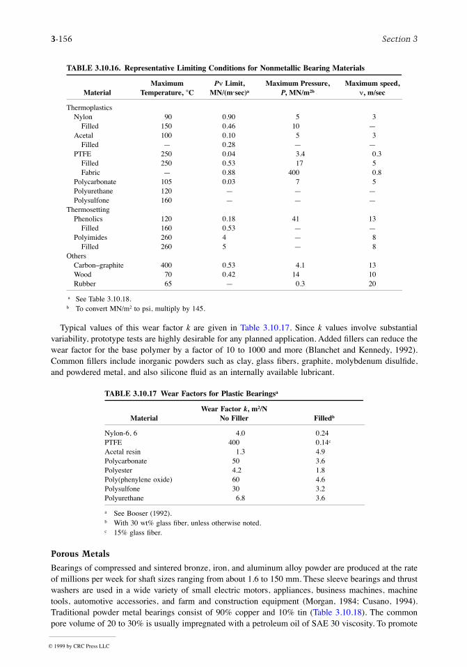
3-156 Section 3
Typical values of this wear factor k are given in Table 3.10.17. Since k values involve substantialvariability, prototype tests are highly desirable for any planned application. Added Þllers can reduce thewear factor for the base polymer by a factor of 10 to 1000 and more (Blanchet and Kennedy, 1992).Common Þllers include inorganic powders such as clay, glass Þbers, graphite, molybdenum disulÞde,and powdered metal, and also silicone ßuid as an internally available lubricant.
Porous Metals
Bearings of compressed and sintered bronze, iron, and aluminum alloy powder are produced at the rateof millions per week for shaft sizes ranging from about 1.6 to 150 mm. These sleeve bearings and thrustwashers are used in a wide variety of small electric motors, appliances, business machines, machinetools, automotive accessories, and farm and construction equipment (Morgan, 1984; Cusano, 1994).Traditional powder metal bearings consist of 90% copper and 10% tin (Table 3.10.18). The commonpore volume of 20 to 30% is usually impregnated with a petroleum oil of SAE 30 viscosity. To promote
TABLE 3.10.16. Representative Limiting Conditions for Nonmetallic Bearing Materials
MaterialMaximum
Temperature, °CPn Limit,
MN/(másec)a
Maximum Pressure, P, MN/m2b
Maximum speed,n, m/sec
ThermoplasticsNylon 90 0.90 5 3
Filled 150 0.46 10 ÑAcetal 100 0.10 5 3
Filled Ñ 0.28 Ñ ÑPTFE 250 0.04 3.4 0.3
Filled 250 0.53 17 5Fabric Ñ 0.88 400 0.8
Polycarbonate 105 0.03 7 5Polyurethane 120 Ñ Ñ ÑPolysulfone 160 Ñ Ñ Ñ
ThermosettingPhenolics 120 0.18 41 13
Filled 160 0.53 Ñ ÑPolyimides 260 4 Ñ 8
Filled 260 5 Ñ 8Others
CarbonÐgraphite 400 0.53 4.1 13Wood 70 0.42 14 10Rubber 65 Ñ 0.3 20
a See Table 3.10.18.b To convert MN/m2 to psi, multiply by 145.
TABLE 3.10.17 Wear Factors for Plastic Bearingsa
Wear Factor k, m2/NMaterial No Filler Filledb
Nylon-6, 6 4.0 0.24PTFE 400 0.14c
Acetal resin 1.3 4.9Polycarbonate 50 3.6Polyester 4.2 1.8Poly(phenylene oxide) 60 4.6Polysulfone 30 3.2Polyurethane 6.8 3.6
a See Booser (1992).b With 30 wt% glass Þber, unless otherwise noted.c 15% glass Þber.
© 1999 by CRC Press LLC
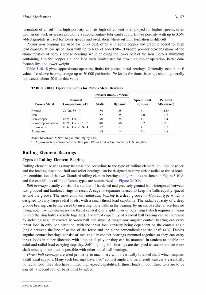
Fluid Mechanics 3-157
formation of an oil Þlm, high porosity with its high oil content is employed for higher speeds, oftenwith an oil wick or grease providing a supplementary lubricant supply. Lower porosity with up to 3.5%added graphite is used for lower speeds and oscillation where oil Þlm formation is difÞcult.
Porous iron bearings are used for lower cost, often with some copper and graphite added for highload capacity at low speed. Iron with up to 40% of added 90Ð10 bronze powder provides many of thecharacteristics of porous bronze bearings while enjoying the lower cost of the iron. Porous aluminumcontaining 3 to 5% copper, tin, and lead Þnds limited use for providing cooler operation, better con-formability, and lower weight.
Table 3.10.18 gives approximate operating limits for porous metal bearings. Generally, maximum Pvalues for sleeve bearings range up to 50,000 psi×ft/min. Pn levels for thrust bearings should generallynot exceed about 20% of this value.
Rolling Element Bearings
Types of Rolling Element Bearings
Rolling element bearings may be classiÞed according to the type of rolling element, i.e., ball or roller,and the loading direction. Ball and roller bearings can be designed to carry either radial or thrust loads,or a combination of the two. Standard rolling element bearing conÞgurations are shown in Figure 3.10.8,and the capabilities of the different types are summarized in Figure 3.10.9.
Ball bearings usually consist of a number of hardened and precisely ground balls interposed betweentwo grooved and hardened rings or races. A cage or separator is used to keep the balls equally spacedaround the groove. The most common radial ball bearing is a deep groove, or Conrad, type which isdesigned to carry large radial loads, with a small thrust load capability. The radial capacity of a deepgroove bearing can be increased by inserting more balls in the bearing, by means of either a face-locatedÞlling notch (which decreases the thrust capacity) or a split inner or outer ring (which requires a meansto hold the ring halves axially together). The thrust capability of a radial ball bearing can be increasedby inducing angular contact between ball and rings. A single-row angular contact bearing can carrythrust load in only one direction, with the thrust load capacity being dependent on the contact angle(angle between the line of action of the force and the plane perpendicular to the shaft axis). Duplexangular contact bearings consist of two angular contact bearings mounted together so they can carrythrust loads in either direction with little axial play, or they can be mounted in tandem to double theaxial and radial load-carrying capacity. Self-aligning ball bearings are designed to accommodate moreshaft misalignment than is possible with other radial ball bearings.
Thrust ball bearings are used primarily in machinery with a vertically oriented shaft which requiresa stiff axial support. Many such bearings have a 90° contact angle and, as a result, can carry essentiallyno radial load; they also have limited high-speed capability. If thrust loads in both directions are to becarried, a second row of balls must be added.
TABLE 3.10.18 Operating Limits for Porous Metal Bearings
Nominal Composition, wt%
Pressure limit, P, MN/m2
Porous Metal Static DynamicSpeed Limit
n, m/secPn Limit
MN/(másec)
Bronze Cu 90, Sn 10 59 28 6.1 1.8a
Iron 52 25 2.0 1.3IronÐcopper Fe 90, Cu 10 140 28 1.1 1.4IronÐcopperÐcarbon Fe 96, Cu 3, C 0.7 340 56 0.2 2.6Bronze-iron Fe 60, Cu 36, Sn 4 72 17 4.1 1.2Aluminum 28 14 6.1 1.8
Note: To convert MN/m2 to psi, multiply by 145.a Approximately equivalent to 50,000 psi á ft/min limit often quoted by U.S. suppliers.
© 1999 by CRC Press LLC
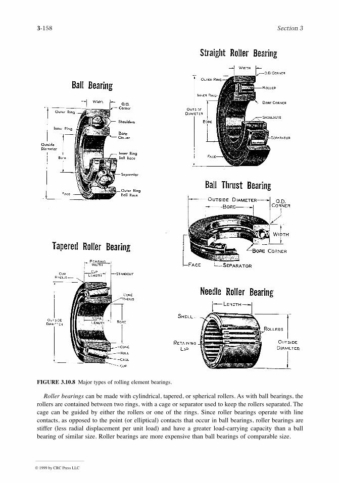
3-158 Section 3
Roller bearings can be made with cylindrical, tapered, or spherical rollers. As with ball bearings, therollers are contained between two rings, with a cage or separator used to keep the rollers separated. Thecage can be guided by either the rollers or one of the rings. Since roller bearings operate with linecontacts, as opposed to the point (or elliptical) contacts that occur in ball bearings, roller bearings arestiffer (less radial displacement per unit load) and have a greater load-carrying capacity than a ballbearing of similar size. Roller bearings are more expensive than ball bearings of comparable size.
FIGURE 3.10.8 Major types of rolling element bearings.
© 1999 by CRC Press LLC
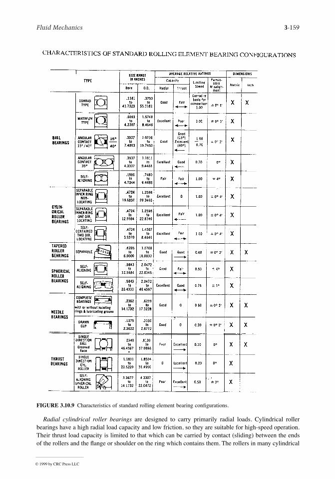
Fluid Mechanics 3-159
Radial cylindrical roller bearings are designed to carry primarily radial loads. Cylindrical rollerbearings have a high radial load capacity and low friction, so they are suitable for high-speed operation.Their thrust load capacity is limited to that which can be carried by contact (sliding) between the endsof the rollers and the ßange or shoulder on the ring which contains them. The rollers in many cylindrical
FIGURE 3.10.9 Characteristics of standard rolling element bearing conÞgurations.
© 1999 by CRC Press LLC
3-160 Section 3
roller bearings are actually slightly crowned to relieve stress concentrations which would otherwise occurat the ends of the rollers and to compensate for misalignment of the bearing. In order to increase theload-carrying capacity of roller bearings, a second row of rollers is added instead of using longer rollers.This is because long rollers (i.e., length/diameter > 1.7) tend to skew in the roller path, thus limitingtheir high-speed capability and sometimes shortening their life. Needle bearings have long rollers,however, and they are useful when there are severe radial space limitations and when neither high loadcapacity nor high speeds are required.
Spherical roller bearings usually have an outer ring with a spherical inside diameter, within whichare barrel-shaped rollers. This makes these bearings self-aligning, and also gives them a larger contactarea between roller and ring than is the case for other rolling element bearings. Because of this, sphericalroller bearings have a very high radial load-carrying capacity, along with some ability to carry thrustloads. They have higher friction between roller and ring, and this limits their high-speed capability.
Tapered roller bearings have tapered rollers, ideally shaped like truncated cones, contained betweentwo mating cones of different angles, the inner cone and the outer cup. The contact angle of the bearingdetermines its thrust load capability; a steeper angle is chosen for more thrust capacity. If a single rowof rollers is used, the bearing is separable and can carry thrust loads in only one direction. If the thrustis double acting, a second bearing can be mounted in a back-to-back conÞguration or a double rowbearing can be selected. In tapered roller bearings there is sliding contact between the ends of the rollersand the guide ßange on the inner cone, and this sliding contact requires lubrication to prevent wear andreduce friction.
Thrust roller bearings can be either cylindrical, needle, tapered, or spherical (Figure 3.10.9). In eachcase there is high load-carrying capacity, but the sliding that occurs between rollers and rings requireslubrication and cooling.
Rolling Element Bearing Materials
Ball and roller bearings require materials with excellent resistance to rolling contact fatigue and wear,as well as good dimensional stability and impact resistance. The rolling elements are subjected to cycliccontact pressures which can range from 70 to 3500 MPa (100 to 500 ksi) or more, and the bearingmaterials must be hard enough to resist surface fatigue under those conditions. Of the through-hardeningsteels which meet these requirements, the most popular is AISI 52100, which contains about 1% carbonand 1.5% chromium. In general, balls and rollers made from 52100 are hardened to about RockwellC60. Standard bearings made from 52100 may suffer from unacceptable dimensional changes resultingfrom metallurgical transformations at operating temperatures above 140°C (285°F). Special stabilizationheat treatments enable operation at higher temperatures, with successful operation at temperatures ashigh as 200°C (390°F) having been achieved in cases involving low loads. The strength and fatigueresistance of the material diminish if the bearing temperature increases above about 175°C (350°F,however, so above that temperature materials with better hot-hardness, such as M50 tool steel, arerequired. Carburizing steels such as AISI 8620 have been developed for tapered roller bearings and otherheavily loaded types that beneÞt from the tougher core and case compressive residual stress developedduring carburizing. For applications in oxidative or corrosive environments, a hardened martensiticstainless steel such as SAE 440C may be chosen. For the highest operating temperatures, ceramicmaterials may be used in bearings. The most promising of the ceramics for rolling element bearingapplications is silicon nitride. Its major use so far in bearings has been in hybrid bearings with ceramicballs or rollers and metallic rings, but all-ceramic bearings have also been developed.
The temperature limits of these bearing materials are given in Table 3.10.19. For all bearing materials,great care must be taken in the processing and production stages to ensure that no defects or inclusionsare present that could serve as an initiation site for fatigue cracks. For most high-performance metallicbearings, this requires a very clean steel production process, such as vacuum arc remelting. Heat treatmentof the material is also important to produce the required dimensional stability. The production processfor ceramic bearings is even more critical, because a defect in a ceramic bearing element could resultin catastrophic fracture of the brittle material.
© 1999 by CRC Press LLC
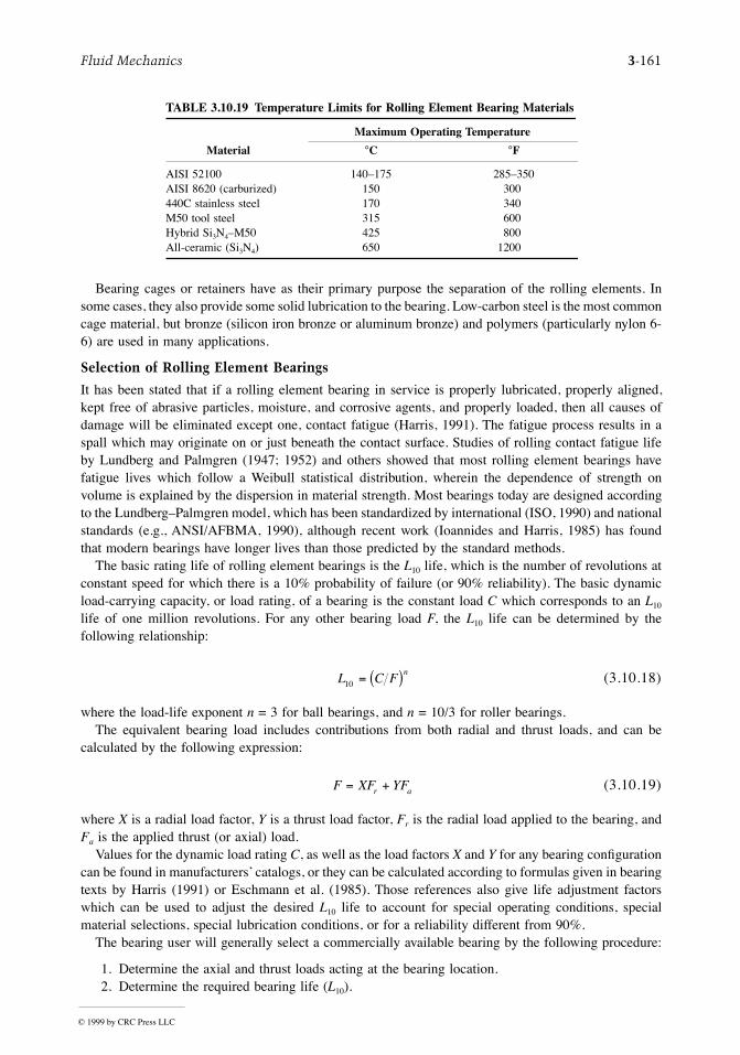
Fluid Mechanics 3-161
Bearing cages or retainers have as their primary purpose the separation of the rolling elements. Insome cases, they also provide some solid lubrication to the bearing. Low-carbon steel is the most commoncage material, but bronze (silicon iron bronze or aluminum bronze) and polymers (particularly nylon 6-6) are used in many applications.
Selection of Rolling Element Bearings
It has been stated that if a rolling element bearing in service is properly lubricated, properly aligned,kept free of abrasive particles, moisture, and corrosive agents, and properly loaded, then all causes ofdamage will be eliminated except one, contact fatigue (Harris, 1991). The fatigue process results in aspall which may originate on or just beneath the contact surface. Studies of rolling contact fatigue lifeby Lundberg and Palmgren (1947; 1952) and others showed that most rolling element bearings havefatigue lives which follow a Weibull statistical distribution, wherein the dependence of strength onvolume is explained by the dispersion in material strength. Most bearings today are designed accordingto the LundbergÐPalmgren model, which has been standardized by international (ISO, 1990) and nationalstandards (e.g., ANSI/AFBMA, 1990), although recent work (Ioannides and Harris, 1985) has foundthat modern bearings have longer lives than those predicted by the standard methods.
The basic rating life of rolling element bearings is the L10 life, which is the number of revolutions atconstant speed for which there is a 10% probability of failure (or 90% reliability). The basic dynamicload-carrying capacity, or load rating, of a bearing is the constant load C which corresponds to an L10
life of one million revolutions. For any other bearing load F, the L10 life can be determined by thefollowing relationship:
(3.10.18)
where the load-life exponent n = 3 for ball bearings, and n = 10/3 for roller bearings.The equivalent bearing load includes contributions from both radial and thrust loads, and can be
calculated by the following expression:
(3.10.19)
where X is a radial load factor, Y is a thrust load factor, Fr is the radial load applied to the bearing, andFa is the applied thrust (or axial) load.
Values for the dynamic load rating C, as well as the load factors X and Y for any bearing conÞgurationcan be found in manufacturersÕ catalogs, or they can be calculated according to formulas given in bearingtexts by Harris (1991) or Eschmann et al. (1985). Those references also give life adjustment factorswhich can be used to adjust the desired L10 life to account for special operating conditions, specialmaterial selections, special lubrication conditions, or for a reliability different from 90%.
The bearing user will generally select a commercially available bearing by the following procedure:
1. Determine the axial and thrust loads acting at the bearing location.2. Determine the required bearing life (L10).
TABLE 3.10.19 Temperature Limits for Rolling Element Bearing Materials
Maximum Operating Temperature
Material °C °F
AISI 52100 140Ð175 285Ð350AISI 8620 (carburized) 150 300440C stainless steel 170 340M50 tool steel 315 600Hybrid Si3N4ÐM50 425 800All-ceramic (Si3N4) 650 1200
L C Fn
10 = ( )
F XF YFr a= +
© 1999 by CRC Press LLC
3-162 Section 3
3. Select the most appropriate bearing type from among those given in Figure 3.10.9.4. Use the X and Y values appropriate to the type of bearing and loading conditions in Equation
(3.10.19) to Þnd the equivalent dynamic bearing load F.5. Determine the required dynamic load capacity C from Equation (3.10.18).6. Select a bearing with a dynamic load capacity at least as large as the required value from a
manufacturerÕs catalog.7. Provide an appropriate mounting arrangement for the bearing. ManufacturersÕ catalogs can be
consulted for guidance in designing the mounting and selecting appropriate Þts for the bearing.The importance of the Þt cannot be overemphasized, since improper Þt can result in considerablereduction in bearing life.
8. Provide adequate lubrication for the bearing (see below). Seals and/or shields may be integratedinto the bearing to retain or protect the lubricant in the bearing.
Rolling Bearing Lubrication
The primary load-carrying contacts between rolling elements and rings exhibit nearly pure rolling. Thereare many sliding contacts in rolling element bearings, however, including those where roller ends contactthe internal ßanges of rings, where rolling elements contact separator/cage, and where the separatorcontacts the guiding (piloting) ring of the bearing. All of those contacts must be lubricated to limitfriction and wear, and either a grease or an oil can be used for that purpose.
Under most normal operating conditions, rolling element bearings can be grease lubricated. Greasescoat surfaces with a thin boundary lubricant Þlm of oil, thickener, and additive molecules, thus providingprotection against sliding wear, and provide oil to lubricate the concentrated rolling contacts (see below).The selection of a grease depends on its effective temperature range, oil viscosity, consistency, and rust-inhibiting properties. For normal applications, a bearing should be Þlled with grease up to 30 to 50%of its free volume. OverÞlling will cause overheating, particularly at high speeds. Grease will deterioratewith time and will leak out. For that reason, there should be a relubrication schedule, with grease beingadded at intervals which can be estimated by the following expression (Neale, 1993):
(3.10.20)
where k = 10 for radial ball bearings, 5 for cylindrical roller bearings, and 1 for spherical or taperedroller bearings; d = bearing bore diameter (mm); and n = speed (rpm)
Oil lubrication is required when high speed or high operating temperatures preclude the use of grease.It is necessary to choose an oil of proper viscosity and appropriate viscosityÐtemperature characteristicsin order to insure sufÞcient thickness of oil Þlm in the lubricated concentrated contacts. If viscosity istoo low, the Þlm thickness will not prevent metal/metal contact, but if the viscosity is too high, excessivefriction will occur. Oil can be applied to a bearing by one of several methods (listed in order of increasingeffectiveness at increasing bearing speed): oil bath, in which the rolling elements carry the oil throughthe bearing; oil circulating system, in which the oil is pumped from the bearing through an externalÞlter and heat exchanger and back to the bearing; oil mist, in which an airstream carries oil droplets tothe bearing; and oil jets, in which the oil is injected into the bearing through carefully positioned nozzles.The quantity and entry velocity of the oil must be carefully selected and controlled in order to dissipatethe heat generated in the bearing.
The lubrication mechanism in the concentrated contacts of rolling element bearings is elastohydro-dynamic lubrication (EHL). EHL typically occurs in lubricated, nonconforming elastic contacts, suchas the elliptical contact that occurs between ball and raceway or the rectangular contact between rollerand ring. These lubricated contacts have a very small area and the contact pressures are very high.Because of those high pressures, the contacting surfaces deform and the lubricant viscosity increases,thereby aiding its ability to sustain heavy loading without oil-Þlm breakdown. A diagram of thesephenomena is shown in Figure 3.10.10. The most important parameter of the concentrated contact, from
relubrication interval hours( ) = ( ) ´( ) -[ ]k d n d1 2 6 1 214 10 4
© 1999 by CRC Press LLC
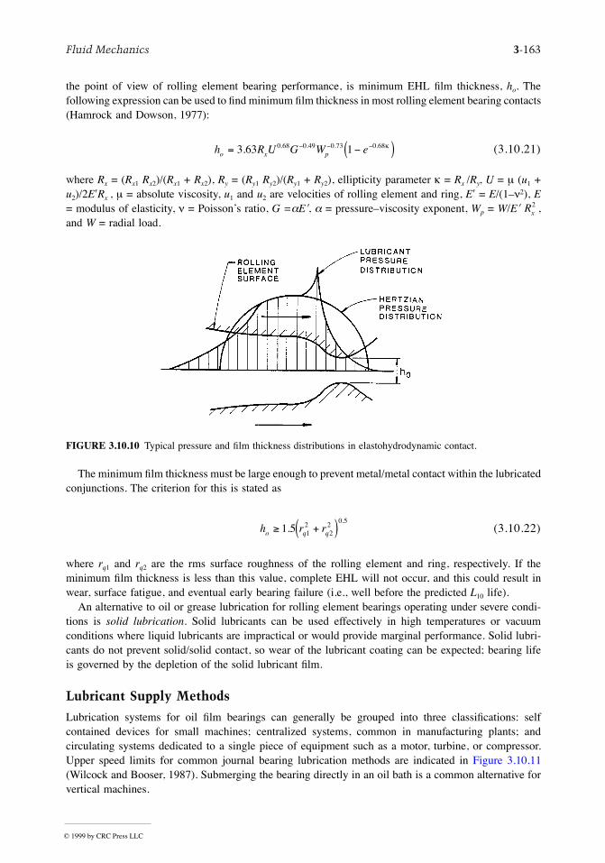
Fluid Mechanics 3-163
the point of view of rolling element bearing performance, is minimum EHL Þlm thickness, ho. Thefollowing expression can be used to Þnd minimum Þlm thickness in most rolling element bearing contacts(Hamrock and Dowson, 1977):
(3.10.21)
where Rx = (Rx1 Rx2)/(Rx1 + Rx2), Ry = (Ry1 Ry2)/(Ry1 + Ry2), ellipticity parameter k = Rx /Ry, U = m (u1 +u2)/2E¢Rx , m = absolute viscosity, u1 and u2 are velocities of rolling element and ring, E¢ = E/(1Ðn2), E= modulus of elasticity, n = PoissonÕs ratio, G =aE¢, a = pressureÐviscosity exponent, Wp = W/E¢ ,and W = radial load.
The minimum Þlm thickness must be large enough to prevent metal/metal contact within the lubricatedconjunctions. The criterion for this is stated as
(3.10.22)
where rq1 and rq2 are the rms surface roughness of the rolling element and ring, respectively. If theminimum Þlm thickness is less than this value, complete EHL will not occur, and this could result inwear, surface fatigue, and eventual early bearing failure (i.e., well before the predicted L10 life).
An alternative to oil or grease lubrication for rolling element bearings operating under severe condi-tions is solid lubrication. Solid lubricants can be used effectively in high temperatures or vacuumconditions where liquid lubricants are impractical or would provide marginal performance. Solid lubri-cants do not prevent solid/solid contact, so wear of the lubricant coating can be expected; bearing lifeis governed by the depletion of the solid lubricant Þlm.
Lubricant Supply Methods
Lubrication systems for oil Þlm bearings can generally be grouped into three classiÞcations: selfcontained devices for small machines; centralized systems, common in manufacturing plants; andcirculating systems dedicated to a single piece of equipment such as a motor, turbine, or compressor.Upper speed limits for common journal bearing lubrication methods are indicated in Figure 3.10.11(Wilcock and Booser, 1987). Submerging the bearing directly in an oil bath is a common alternative forvertical machines.
FIGURE 3.10.10 Typical pressure and Þlm thickness distributions in elastohydrodynamic contact.
h R U G W eo x p= -( )- - -3 63 10 68 0 49 0 73 0 68. . . . . k
Rx2
h r ro q q³ +( )1 5 12
22
0 5.
.
© 1999 by CRC Press LLC
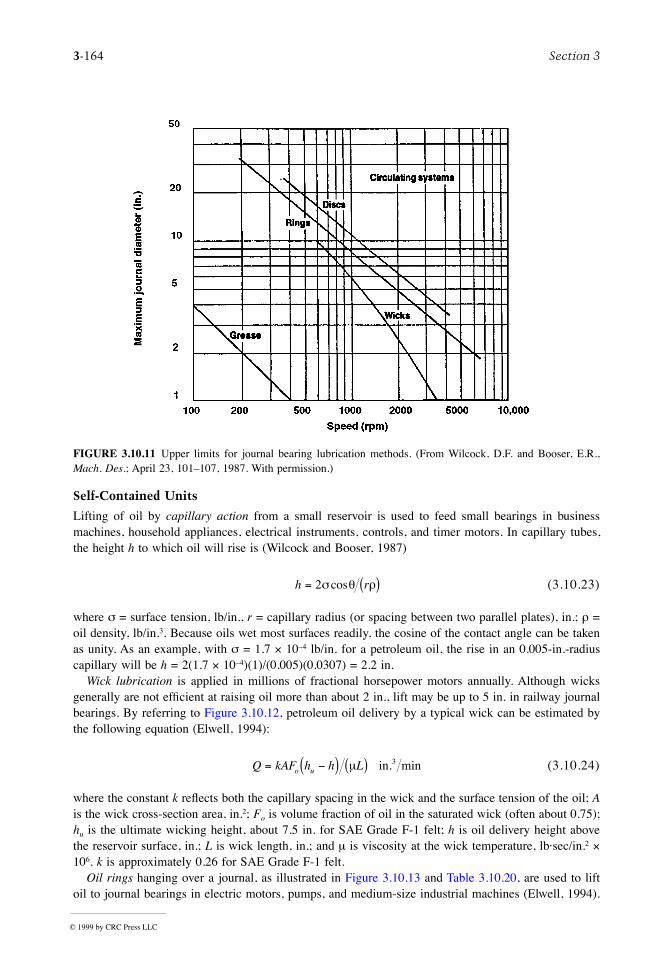
3-164 Section 3
Self-Contained Units
Lifting of oil by capillary action from a small reservoir is used to feed small bearings in businessmachines, household appliances, electrical instruments, controls, and timer motors. In capillary tubes,the height h to which oil will rise is (Wilcock and Booser, 1987)
(3.10.23)
where s = surface tension, lb/in., r = capillary radius (or spacing between two parallel plates), in.; r =oil density, lb/in.3. Because oils wet most surfaces readily, the cosine of the contact angle can be takenas unity. As an example, with s = 1.7 ´ 10Ð4 lb/in. for a petroleum oil, the rise in an 0.005-in.-radiuscapillary will be h = 2(1.7 ´ 10Ð4)(1)/(0.005)(0.0307) = 2.2 in.
Wick lubrication is applied in millions of fractional horsepower motors annually. Although wicksgenerally are not efÞcient at raising oil more than about 2 in., lift may be up to 5 in. in railway journalbearings. By referring to Figure 3.10.12, petroleum oil delivery by a typical wick can be estimated bythe following equation (Elwell, 1994):
(3.10.24)
where the constant k reßects both the capillary spacing in the wick and the surface tension of the oil; Ais the wick cross-section area, in.2; Fo is volume fraction of oil in the saturated wick (often about 0.75);hu is the ultimate wicking height, about 7.5 in. for SAE Grade F-1 felt; h is oil delivery height abovethe reservoir surface, in.; L is wick length, in.; and m is viscosity at the wick temperature, lbásec/in.2 ´106. k is approximately 0.26 for SAE Grade F-1 felt.
Oil rings hanging over a journal, as illustrated in Figure 3.10.13 and Table 3.10.20, are used to liftoil to journal bearings in electric motors, pumps, and medium-size industrial machines (Elwell, 1994).
FIGURE 3.10.11 Upper limits for journal bearing lubrication methods. (From Wilcock, D.F. and Booser, E.R.,Mach. Des.; April 23, 101Ð107, 1987. With permission.)
h r= ( )2s q rcos
Q kAF h h Lo u= -( ) ( )m in.3 min
© 1999 by CRC Press LLC
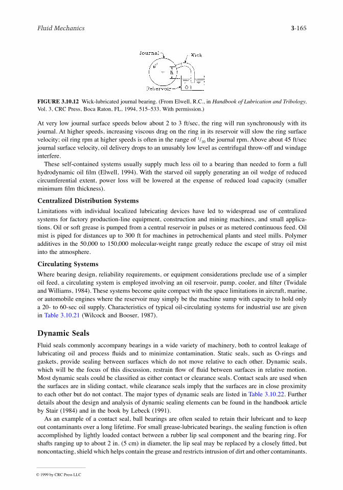
Fluid Mechanics 3-165
At very low journal surface speeds below about 2 to 3 ft/sec, the ring will run synchronously with itsjournal. At higher speeds, increasing viscous drag on the ring in its reservoir will slow the ring surfacevelocity; oil ring rpm at higher speeds is often in the range of 1/10 the journal rpm. Above about 45 ft/secjournal surface velocity, oil delivery drops to an unusably low level as centrifugal throw-off and windageinterfere.
These self-contained systems usually supply much less oil to a bearing than needed to form a fullhydrodynamic oil Þlm (Elwell, 1994). With the starved oil supply generating an oil wedge of reducedcircumferential extent, power loss will be lowered at the expense of reduced load capacity (smallerminimum Þlm thickness).
Centralized Distribution Systems
Limitations with individual localized lubricating devices have led to widespread use of centralizedsystems for factory production-line equipment, construction and mining machines, and small applica-tions. Oil or soft grease is pumped from a central reservoir in pulses or as metered continuous feed. Oilmist is piped for distances up to 300 ft for machines in petrochemical plants and steel mills. Polymeradditives in the 50,000 to 150,000 molecular-weight range greatly reduce the escape of stray oil mistinto the atmosphere.
Circulating Systems
Where bearing design, reliability requirements, or equipment considerations preclude use of a simpleroil feed, a circulating system is employed involving an oil reservoir, pump, cooler, and Þlter (Twidaleand Williams, 1984). These systems become quite compact with the space limitations in aircraft, marine,or automobile engines where the reservoir may simply be the machine sump with capacity to hold onlya 20- to 60-sec oil supply. Characteristics of typical oil-circulating systems for industrial use are givenin Table 3.10.21 (Wilcock and Booser, 1987).
Dynamic Seals
Fluid seals commonly accompany bearings in a wide variety of machinery, both to control leakage oflubricating oil and process ßuids and to minimize contamination. Static seals, such as O-rings andgaskets, provide sealing between surfaces which do not move relative to each other. Dynamic seals,which will be the focus of this discussion, restrain ßow of ßuid between surfaces in relative motion.Most dynamic seals could be classiÞed as either contact or clearance seals. Contact seals are used whenthe surfaces are in sliding contact, while clearance seals imply that the surfaces are in close proximityto each other but do not contact. The major types of dynamic seals are listed in Table 3.10.22. Furtherdetails about the design and analysis of dynamic sealing elements can be found in the handbook articleby Stair (1984) and in the book by Lebeck (1991).
As an example of a contact seal, ball bearings are often sealed to retain their lubricant and to keepout contaminants over a long lifetime. For small grease-lubricated bearings, the sealing function is oftenaccomplished by lightly loaded contact between a rubber lip seal component and the bearing ring. Forshafts ranging up to about 2 in. (5 cm) in diameter, the lip seal may be replaced by a closely Þtted, butnoncontacting, shield which helps contain the grease and restricts intrusion of dirt and other contaminants.
FIGURE 3.10.12 Wick-lubricated journal bearing. (From Elwell, R.C., in Handbook of Lubrication and Tribology,Vol. 3, CRC Press, Boca Raton, FL, 1994, 515Ð533. With permission.)
© 1999 by CRC Press LLC
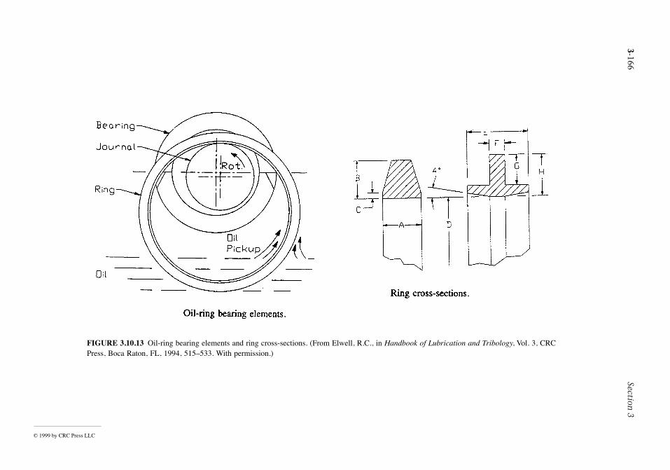
3-166Section
3
© 1999 by CRC Press LLC
FIG in Handbook of Lubrication and Tribology, Vol. 3, CRCPres
URE 3.10.13 Oil-ring bearing elements and ring cross-sections. (From Elwell, R.C.,s, Boca Raton, FL, 1994, 515Ð533. With permission.)
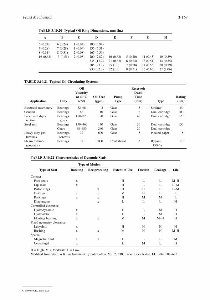
Fluid Mechanics 3-167
TABLE 3.10.20 Typical Oil-Ring Dimensions, mm (in.)
A B C D E F G H
6 (0.24) 6 (0.24) 1 (0.04) 100 (3.94)7 (0.28) 7 (0.28) 1 (0.04) 135 (5.31)8 (0.31) 8 (0.31) 2 (0.08) 165 (6.50)16 (0.63) 13 (0.51) 2 (0.08) 200 (7.87) 16 (0.63) 5 (0.20) 11 (0.43) 10 (0.39)
335 (13.2) 21 (0.83) 6 (0.24) 13 (0.51) 14 (0.55)585 (23.0) 25 (1.0) 7 (0.28) 14 (0.55) 20 (0.79)830 (32.7) 32 (1.3) 8 (0.31) 16 (0.63) 27 (1.06)
TABLE 3.10.21 Typical Oil Circulating Systems
Application Duty
Oil Viscosityat 40°C
(cSt)Oil Feed
(gpm)Pump Type
Reservoir Dwell Time (min) Type
Rating (mm)
Electrical machinery Bearings 32Ð68 2 Gear 5 Strainer 50General Bearings 68 10 Gear 8 Dual cartridge 100Paper mill dryer section
Bearings, gears
150Ð220 20 Gear 40 Dual cartridge 120
Steel mill Bearings 150Ð460 170 Gear 30 Dual cartridge 150Gears 68Ð680 240 Gear 20 Dual cartridge
Heavy duty gas turbines
Bearings,controls
32 600 Gear 5 Pleated paper 5
Steam turbine-generators
Bearings 32 1000 Centrifugal 5 Bypass 15%/hr
10
TABLE 3.10.22 Characteristics of Dynamic Seals
Type of Motion
Type of Seal Rotating Reciprocating Extent of Use Friction Leakage Life
ContactFace seals x H L L MÐHLip seals x H L L LÐMPiston rings x H H L LÐMO-Rings x x M H L LPackings x x H M M LDiaphragms x L L L H
Controlled clearanceHydrodynamic x L L M HHydrostatic x L L M HFloating bushing x x M M MÐH H
Fixed geometry clearanceLabyrinth x H H H HBushing x x M H H MÐH
SpecialMagnetic ßuid x x L L L MCentrifugal x L M L H
H = High, M = Moderate, L = Low.ModiÞed from Stair, W.K., in Handbook of Lubrication, Vol. 2, CRC Press, Boca Raton, FL 1984, 581Ð622.
© 1999 by CRC Press LLC
3-168 Section 3
For more severe sealing requirements in rolling element bearings, labyrinth clearance seals may be used(Harris, 1991).
The most common seals for rotating shafts passing through Þxed housings, such as pumps or gear-boxes, are radial lip seals and mechanical face seals. These contact seals can be designed to handle awide range of sealed ßuids, temperatures, velocities, and pressures (Stair, 1984; Lebeck, 1991). Materialselection and surface Þnish considerations are similar to those discussed in the subsections on slidingfriction and its consequences and on dry and semilubricated bearings.
When high surface speeds are encountered, wear and frictional heating may prohibit use of rubbingcontact seals. For such applications, clearance seals such as close-Þtting labyrinth seals or controlled-clearance ßuid Þlm seals can be used. Fluid Þlm seals can be either hydrostatic or hydrodynamic; bothtypes have a pressurized Þlm of ßuid which prevents contact between the sealed surfaces and use pressurebalancing to restrain leakage. The principles governing their operation are similar to those discussed inthe subsection on ßuid Þlm bearings. Details of ßuid Þlm seals can be found in Shapiro (1995).
References
ANSI/AFBMA, 1990. Load Ratings and Fatigue Life for Ball Bearings, ANSI/AFBMA 9Ð1990,AFBMA, Washington, D.C.
Archard, J.F. 1980. Wear theory and mechanisms, in Wear Control Handbook, M.B. Peterson and W.O.Winer, Eds., ASME, New York.
Bhushan, B. and Gupta, B.K. 1991. Handbook of Tribology, McGraw-Hill, New York.Blanchet, T.A. and Kennedy, F.E. 1992. Sliding wear mechanism of polytetraßuoroethylene (PTFE) and
PTFE composites, Wear, 153:229Ð243.Blau, P.J., Ed. 1992. Friction, Lubrication and Wear Technology, Metals Handbook, Vol. 18, 10th ed.,
ASM International, Metals Park, OH.Booser, E.R. 1992. Bearing materials, in Encyclopedia of Chemical Technology, Vol. 4, pp. 1Ð21, John
Wiley & Sons, New York.Booser, E.R. 1995. Lubricants and lubrication, in Encyclopedia of Chemical Technology, 4th ed., Vol.
15, pp. 463Ð517, John Wiley & Sons, New York.Booser, E.R. and Wilcock, D.F. 1987. New technique simpliÞes journal bearing design, Mach. Des.,
April 23, pp. 101Ð107.Booser, E.R. and Wilcock, D.F. 1991. Selecting thrust bearings, Mach. Des., June 20, pp. 69Ð72.Crook, P. and Farmer, H.N. 1992. Friction and wear of hardfacing alloys, in Friction, Lubrication and
Wear Technology, Metals Handbook, Vol. 18, pp. 758Ð765, ASM International, Metals Park, OH.Cusano, C. 1994. Porous metal bearings, in Handbook of Lubrication and Tribology, Vol. 3, pp. 491Ð513,
CRC Press, Boca Raton, FL.DeHart, A.O. 1984. Sliding bearing materials, in Handbook of Lubrication, Vol. 2, pp. 463Ð476, CRC
Press, Boca Raton, FL.Derner, W.J. and Pfaffenberger, E.E. 1984. Rolling element bearings, in Handbook of Lubrication, Vol.
2, pp. 495, CRC Press, Boca Raton, FL.Elwell, R.C. 1994. Self-contained bearing lubrication: rings, disks, and wicks, in Handbook of Lubri-
cation and Tribology, Vol. 3, pp. 515Ð533, CRC Press, Boca Raton, FL.Engineering Sciences Data Unit (ESDU). 1965. General Guide to the Choice of Journal Bearing Type,
Item 65007, Institution of Mechanical Engineers, London.Engineering Sciences Data Unit (ESDU). 1967. General Guide to the Choice of Thrust Bearing Type,
Item 67073, Institution of Mechanical Engineers, London.Eschmann, P., Hasbargen, L., and Weigand, K. 1985. Ball and Roller Bearings, John Wiley & Sons,
New York.Fenske, G.R. 1992. Ion implantation, in Friction, Lubrication and Wear Technology, Metals Handbook,
Vol. 18, pp. 850Ð860, ASM International, Metals Park, OH.
© 1999 by CRC Press LLC
Fluid Mechanics 3-169
Fuller, D.D. 1984. Theory and practice of lubrication for engineers, 2nd ed., John Wiley & Sons, NewYork.
Hamrock, B. and Dowson, D. 1977. Isothermal elastohydrodynamic lubrication of point contacts, ASMEJ. Lubr. Technol., 99(2): 264Ð276.
Harris, T.A. 1991. Rolling Bearing Analysis, 3rd ed., John Wiley & Sons, New York.Ioannides, S. and Harris, T.A. 1985. A new fatigue life model for rolling bearings, ASME J. Tribology,
107:367Ð378.ISO, 1990. Rolling Bearings Dynamic Load Ratings and Rating Life, International Standard ISO 281.Jamison, W.E. 1994. Plastics and plastic matrix composites, in Handbook of Lubrication and Tribology,
Vol. 3, pp. 121Ð147, CRC Press, Boca Raton, FL.Khonsari, M.M. 1997. In Tribology Data Handbook, CRC Press, Boca Raton, FL.Kingsbury, G.R. 1992. Friction and wear of sliding bearing materials, in ASM Handbook, Vol. 18 pp.
741Ð757, ASM International, Metals Park, OH.Klaus, E.E. and Tewksbury, E.J. 1984. Liquid lubricants, in Handbook of Lubrication, Vol. 2, pp.
229Ð254, CRC Press, Boca Raton, FL.Kushner, B.A. and Novinski, E.R. 1992. Thermal spray coatings, in Friction, Lubrication and Wear
Technology, Metals Handbook, Vol. 18, pp. 829Ð833, ASM International, Metals Park, OH.Lebeck, A.O. 1991. Principles and Design of Mechanical Face Seals, John Wiley & Sons, New York.Lundberg, G. and Palmgren, A. 1947. Dynamic capacity of rolling bearings, Acta Polytech. Mech. Eng.
Ser., 1(3):196.Lundberg, G. and Palmgren, A. 1952. Dynamic capacity of roller bearings, Acta Polytech. Mech. Eng.
Ser., 2(4):210.Morgan, V.T. 1984. Porous Metal Bearings and Their Application, MEP-213, Mechanical Engineering
Publications, Workington, U.K.Neale, M.J. 1993. Bearings, Butterworth-Heinemann, Oxford.Neale, P.B. 1970. J. Mech. Eng. Sci., 12:73Ð84.Peterson, M.B. and Winer, W.O., Eds., 1980. Wear Control Handbook, ASME, New York.Rabinowicz, E. 1980. Wear coefÞcients metals, in Wear Control Handbook, M.B. Peterson and W.O.
Winer, Eds., pp. 475Ð506, ASME, New York.Rabinowicz, E. 1995. Friction and Wear of Materials, 2nd ed., John Wiley & Sons, New York.Ramondi, A.A. and Szeri, A.Z. 1984. Journal and thrust bearings, in Handbook of Lubrication, Vol. 2,
pp. 413Ð462, CRC Press, Boca Raton, FL.Reynolds, O. 1886. On the theory of lubrication and its application to Mr. Beauchamp TowerÕs experi-
ments, Philos. Trans R. Soc., 177:157Ð234.Schmitt, G.F. 1980. Liquid and solid particles impact erosion, in Wear Control Handbook, M.B. Peterson
and W.O. Winer, Eds., pp. 231Ð282, ASME, New York.Shabel, B.S. Granger, D.A., and Tuckner, W.G. 1992. Friction and wear of aluminumÐsilicon alloys, in
ASM Handbook, Vol. 18, pp. 785Ð794, ASM International, Metals Park, OH.Shapiro, W. 1995. Hydrodynamic and hydrostatic seals, in Handbook of Lubrication and Tribology, Vol.
3, pp. 445Ð468, CRC Press, Boca Raton, FL.Stair, W.K. 1984. Dynamic seals, in Handbook of Lubrication, Vol. 2, pp. 581Ð622, CRC Press, Boca
Raton, FL.Twidale, A.J. and Williams, D.C.J. 1984. Circulating oil systems, in Handbook of Lubrication, Vol. 2,
pp. 395Ð409, CRC Press, Boca Raton, FL.Weil, R. and Sheppard, K. 1992. Electroplated coatings, in Friction, Lubrication and Wear Technology,
Metals Handbook, Vol. 18, pp. 834Ð839, ASM International, Ohio. Wilcock, D.F. and Booser, E.R. 1956. Bearing design and application, McGraw-Hill, New York.Wilcock, D.F. and Booser, E.R. 1987. Lubrication techniques for journal bearings, Machine Des., April
23, 101Ð107.
© 1999 by CRC Press LLC
3-170 Section 3
3.11 Pumps and Fans
Robert F. Boehm
Introduction
Pumps are devices that impart a pressure increase to a liquid. Fans are used to increase the velocity ofa gas, but this is also accomplished through an increase in pressure. The pressure rise found in pumpscan vary tremendously, and this is a very important design parameter along with the liquid ßow rate.This pressure rise can range from simply increasing the elevation of the liquid to increasing the pressurehundreds of atmospheres. Fan applications, on the other hand, generally deal with small pressureincreases. In spite of this seemingly signiÞcant distinction between pumps and fans, there are manysimilarities in the fundamentals of certain types of these machines as well as with their application andtheory of operation.
The appropriate use of pumps and fans depends upon the proper choice of device and the properdesign and installation for the application. A check of sources of commercial equipment shows thatmany varieties of pumps and fans exist. Each of these had special characteristics that must be appreciatedfor achieving proper function. Preliminary design criteria for choosing between different types is givenby Boehm (1987).
As is to be expected, the wise applications of pumps and fans requires knowledge of ßuid ßowfundamentals. Unless the ßuid mechanics of a particular application are understood, the design couldbe less than desirable.
In this section, pump and fan types are brießy deÞned. In addition, typical application information isgiven. Also, some ideas from ßuid mechanics that are especially relevant to pump and fan operation arereviewed.
Pumps
Raising of water from wells and cisterns is the earliest form of pumping (a very detailed history of earlyapplications is given by Ewbank, 1842). Modern applications are much broader, and these Þnd a widevariety of machines in use. Modern pumps function on one of two principles. By far the majority ofpump installations are of the velocity head type. In these devices, the pressure rise is achieved by givingthe ßuid a movement. At the exit of the machine, this movement is translated into a pressure increase.The other major type of pump is called positive displacement. These devices are designed to increasethe pressure of the liquid while essentially trying to compress the volume. A categorization of pumptypes has been given by Krutzsch (1986), and an adaptation of this is shown below.
I. Velocity headA. Centrifugal
1. Axial ßow (single or multistage)2. Radial ßow (single or double suction)3. Mixed ßow (single or double suction)4. Peripheral (single or multistage)
B. Special Effect1. Gas lift2. Jet3. Hydraulic ram4. Electromagnetic
II. Positive displacementA. Reciprocating
1. Piston, plungera. Direct acting (simplex or duplex)
© 1999 by CRC Press LLC
Fluid Mechanics 3-171
b. Power (single or double acting, simplex, duplex, triplex, multiplex)2. Diaphragm (mechanically or ßuid driven, simplex or multiplex)
B. Rotary1. Single rotor (vane, piston, screw, ßexible member, peristaltic)2. Multiple rotor (gear, lobe, screw, circumferential piston)
In the next subsection, some of the more common pumps are described.
Centrifugal and Other Velocity Head Pumps
Centrifugal pumps are used in more industrial applications than any other kind of pump. This is primarilybecause these pumps offer low initial and upkeep costs. Traditionally, pumps of this type have beenlimited to low-pressure-head applications, but modern pump designs have overcome this problem unlessvery high pressures are required. Some of the other good characteristics of these types of devices includesmooth (nonpulsating) ßow and the ability to tolerate nonßow conditions.
The most important parts of the centrifugal pump are the impeller and volute. An impeller can takeon many forms, ranging from essentially a spinning disk to designs with elaborate vanes. The latter isusual. Impeller design tends to be somewhat unique to each manufacturer, as well as Þnding a varietyof designs for a variety of applications. An example of an impeller is shown in Figure 3.11.1. This deviceimparts a radial velocity to the ßuid that has entered the pump perpendicular to the impeller. The volute(there may be one or more) performs the function of slowing the ßuid and increasing the pressure. Agood discussion of centrifugal pumps is given by Lobanoff and Ross (1992).
A very important factor in the speciÞcation of a centrifugal pump is the casing orientation and type.For example, the pump can be oriented vertically or horizontally. Horizontal mounting is most common.Vertical pumps usually offer beneÞts related to ease of priming and reduction in required net positivesuction head (see discussion below). This type also requires less ßoor space. Submersible and immersiblepumps are always of the vertical type. Another factor in the design is the way the casing is split, andthis has implications about ease of manufacture and repair. Casings that are split perpendicular to theshaft are called radially split, while those split parallel to the shaft axis are denoted as axially split. Thelatter can be horizontally split or vertically split. The number of stages in the pump greatly affects thepump-output characteristics. Several stages can be incorporated into the same casing, with an associatedincrease in pump output. Multistage pumps are often used for applications with total developed headover 50 atm.
Whether or not a pump is self-priming can be important. If a centrifugal pump is Þlled with air whenit is turned on, the initiation of pumping action may not be sufÞcient to bring the ßuid into the pump.Pumps can be speciÞed with features that can minimize priming problems.
There are other types of velocity head pumps. Jet pumps increase pressure by imparting momentumfrom a high-velocity liquid stream to a low-velocity or stagnant body of liquid. The resulting ßow then
FIGURE 3.11.1. A schematic of a centrifugal pump is shown. The liquid enters perpendicular to the Þgure, and aradial velocity is imparted by clockwise spin of the impeller.
© 1999 by CRC Press LLC
3-172 Section 3
goes through a diffuser to achieve an overall pressure increase. Gas lifts accomplish a pumping actionby a drag on gas bubbles that rise through a liquid.
Positive-Displacement Pumps
Positive-displacement pumps demonstrate high discharge pressures and low ßow rates. Usually, this isaccomplished by some type of pulsating device. A piston pump is a classic example of positive-displacement machines. Rotary pumps are one type of positive-displacement device that do not impartpulsations to the existing ßow (a full description of these types of pumps is given by Turton, 1994).Several techniques are available for dealing with pulsating ßows, including use of double-acting pumps(usually of the reciprocating type) and installation of pulsation dampeners.
Positive-displacement pumps usually require special seals to contain the ßuid. Costs are higher bothinitially and for maintenance compared with most pumps that operate on the velocity head basis. Positive-displacement pumps demonstrate an efÞciency that is nearly independent of ßow rate, in contrast to thevelocity head type (see Figure 3.11.2 and the discussion related to it below).
Reciprocating pumps offer very high efÞciencies, reaching 90% in larger sizes. These types of pumpsare more appropriate for pumping abrasive liquids (e.g., slurries) than are centrifugal pumps.
A characteristic of positive displacement pumps which may be valuable is that the output ßow isproportional to pump speed. This allows this type of pump to be used for metering applications. Also apositive aspect of these pumps is that they are self-priming, except at initial start-up.
Very high head pressures (often damaging to the pump) can be developed in positive-displacementpumps if the downstream ßow is blocked. For this reason, a pressure-relief-valve bypass must alwaysbe used with positive-displacement pumps.
Pump/Flow Considerations
Performance characteristics of the pump must be considered in system design. Simple diagrams of pumpapplications are shown in Figure 3.11.2. First, consider the left-hand Þgure. This represents a ßow circuit,and the pressure drops related to the piping, Þttings, valves, and any other ßow devices found in thecircuit must be estimated using the laws of ßuid mechanics. Usually, these resistances (pressure drops)are found to vary approximately with the square of the liquid ßow rate. Typical characteristics are shownin Figure 3.11.3. Most pumps demonstrate a ßow vs. pressure rise variation that is a positive value atzero ßow and decreases to zero at some larger ßow. Positive-displacement pumps, as shown on the right-hand side of Figure 3.11.3, are an exception to this in that these devices usually cannot tolerate a zeroßow. An important aspect to note is that a closed system can presumably be pressurized. A contrastingsituation and its implications are discussed below.
The piping diagram show on the right-hand side of Figure 3.11.2 is a once-through system, anotherfrequently encountered installation. However, the leg of piping through Òpressure drop 1Ó shown therecan have some very important implications related to net positive suction head, often denoted as NPSH.In simple terms, NPSH indicates the difference between the local pressure and the thermodynamicsaturation pressure at the ßuid temperature. If NPSH = 0, the liquid can vaporize, and this can result ina variety of outcomes from noisy pump operation to outright failure of components. This condition iscalled cavitation. Cavitation, if it occurs, will Þrst take place at the lowest pressure point within thepiping arrangement. Often this point is located at, or inside, the inlet to the pump. Most manufacturersspecify how much NPSH is required for satisfactory operation of their pumps. Hence, the actual NPSH(denoted as NPSHA) experienced by the pump must be larger than the manufacturerÕs required NPSH(called NPSHR). If a design indicates insufÞcient NPSH, changes should be made in the system, possiblyincluding alternative piping layout, including elevation and/or size, or use of a pump with smaller NPSHrequirements.
The manufacturer should be consulted for a map of operational information for a given pump. Atypical form is shown in Figure 3.11.4. This information will allow the designer to select a pump thatsatisÞed the circuit operational requirements while meeting the necessary NPSH and most-efÞcient-operation criteria.
© 1999 by CRC Press LLC
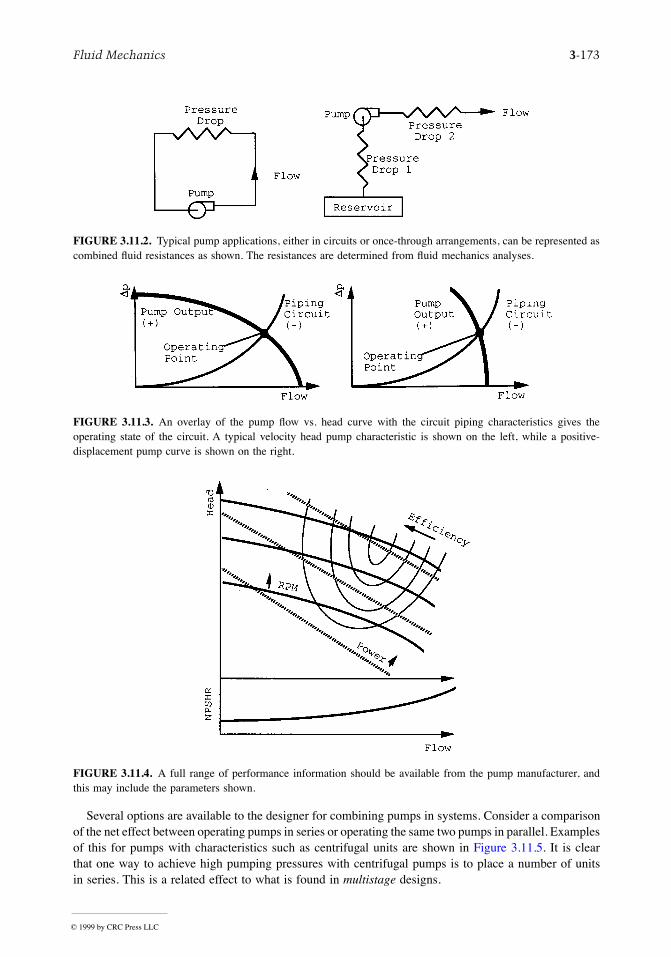
Fluid Mechanics 3-173
Several options are available to the designer for combining pumps in systems. Consider a comparisonof the net effect between operating pumps in series or operating the same two pumps in parallel. Examplesof this for pumps with characteristics such as centrifugal units are shown in Figure 3.11.5. It is clearthat one way to achieve high pumping pressures with centrifugal pumps is to place a number of unitsin series. This is a related effect to what is found in multistage designs.
FIGURE 3.11.2. Typical pump applications, either in circuits or once-through arrangements, can be represented ascombined ßuid resistances as shown. The resistances are determined from ßuid mechanics analyses.
FIGURE 3.11.3. An overlay of the pump ßow vs. head curve with the circuit piping characteristics gives theoperating state of the circuit. A typical velocity head pump characteristic is shown on the left, while a positive-displacement pump curve is shown on the right.
FIGURE 3.11.4. A full range of performance information should be available from the pump manufacturer, andthis may include the parameters shown.
© 1999 by CRC Press LLC
3-174 Section 3
Fans
As noted earlier, fans are devices that cause air to move. This deÞnition is broad and can include aßapping palm branch, but the discussion here deals only with devices that impart air movement due torotation of an impeller inside a Þxed casing. In spite of this limiting deÞnition, a large variety ofcommercial designs are included.
Fans Þnd application in many engineering systems. Along with the chillers and boilers, they are theheart of heating, ventilating, and air conditioning (HVAC) systems. When large physical dimensions ofa unit are not a design concern (usually the case), centrifugal fans are favored over axial ßow units forHVAC applications. Many types of fans are found in power plants. Very large fans are used to furnishair to the boiler, as well as to draw or force air through cooling towers and pollution-control equipment.Electronic cooling Þnds applications for small units. Even automobiles have several fans in them. Becauseof the great engineering importance of fans, several organizations publish rating and testing criteria (see,for example, ASME, 1990).
Generally fans are classiÞed according to how the air ßows through the impeller. These ßows maybe axial (essentially a propeller in a duct), radial (conceptually much like the centrifugal pumps discussedearlier), mixed, and cross. While there are many other fan designations, all industrial units Þt one ofthese classiÞcations. Mixed-ßow fans are so named because both axial and radial ßow occur on thevanes. Casings for these devices are essentially like those for axial-ßow machines, but the inlet has aradial-ßow component. On cross-ßow impellers, the gas traverses the blading twice.
Characteristics of fans are shown in Figure 3.11.6. Since velocities can be high in fans, often boththe total and the static pressure increases are considered. While both are not shown on this Þgure, thecurves have similar variations. Of course the total DP will be greater than will the static value, thedifference being the velocity head. This difference increases as the volume ßow increases. At zero ßow(the shutoff point), the static and total pressure difference values are the same. EfÞciency variation showsa sharp optimum value at the design point. For this reason, it is critical that fan designs be carefullytuned to the required conditions.
A variety of vane type are found on fans, and the type of these is also used for fan classiÞcation.Axial fans usually have vanes of airfoil shape or vanes of uniform thickness. Some vane types that mightbe found on a centrifugal (radial-ßow) fan are shown in Figure 3.11.7.
One aspect that is an issue in choosing fans for a particular application is fan efÞciency. TypicalefÞciency comparisons of the effect of blade type on a centrifugal fan are shown in Figure 3.11.8. Sincevelocities can be high, the value of aerodynamic design is clear. Weighing against this are cost and otherfactors.
An additional aspect that may be important in the choice of fans is noise generation. This may bemost critical in HVAC applications. It is difÞcult to describe noise characteristics in brief terms becauseof the frequency-dependent nature of these phenomena. However, a comparison of speciÞc sound power
FIGURE 3.11.5. Series (a) and parallel (b) operation of centrifugal pumps are possible. The resultant characteristicsfor two identical pumps are shown.
© 1999 by CRC Press LLC
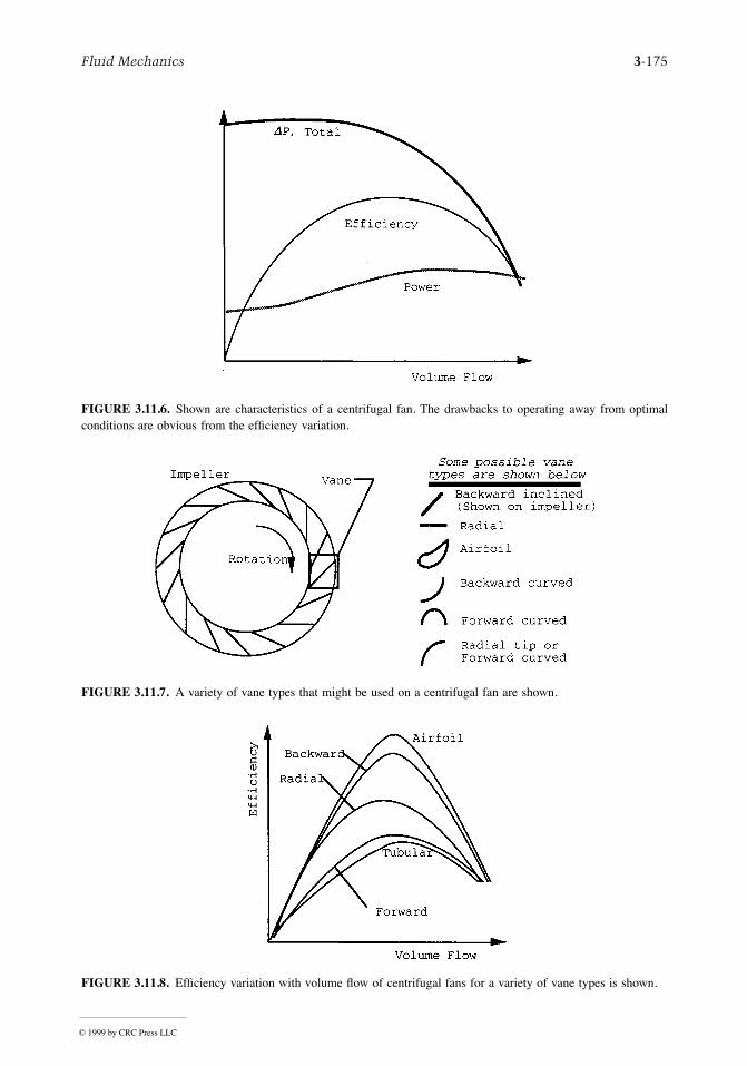
Fluid Mechanics 3-175
FIGURE 3.11.6. Shown are characteristics of a centrifugal fan. The drawbacks to operating away from optimalconditions are obvious from the efÞciency variation.
FIGURE 3.11.7. A variety of vane types that might be used on a centrifugal fan are shown.
FIGURE 3.11.8. EfÞciency variation with volume ßow of centrifugal fans for a variety of vane types is shown.
© 1999 by CRC Press LLC
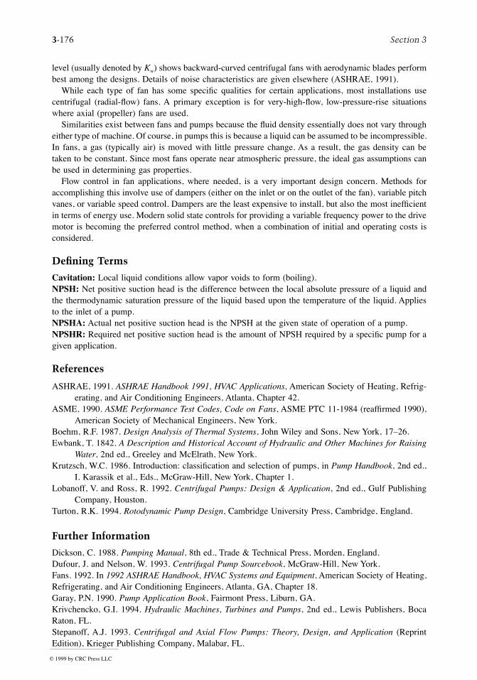
3-176 Section 3
level (usually denoted by Kw) shows backward-curved centrifugal fans with aerodynamic blades performbest among the designs. Details of noise characteristics are given elsewhere (ASHRAE, 1991).
While each type of fan has some speciÞc qualities for certain applications, most installations usecentrifugal (radial-ßow) fans. A primary exception is for very-high-ßow, low-pressure-rise situationswhere axial (propeller) fans are used.
Similarities exist between fans and pumps because the ßuid density essentially does not vary througheither type of machine. Of course, in pumps this is because a liquid can be assumed to be incompressible.In fans, a gas (typically air) is moved with little pressure change. As a result, the gas density can betaken to be constant. Since most fans operate near atmospheric pressure, the ideal gas assumptions canbe used in determining gas properties.
Flow control in fan applications, where needed, is a very important design concern. Methods foraccomplishing this involve use of dampers (either on the inlet or on the outlet of the fan), variable pitchvanes, or variable speed control. Dampers are the least expensive to install, but also the most inefÞcientin terms of energy use. Modern solid state controls for providing a variable frequency power to the drivemotor is becoming the preferred control method, when a combination of initial and operating costs isconsidered.
Defining Terms
Cavitation: Local liquid conditions allow vapor voids to form (boiling).NPSH: Net positive suction head is the difference between the local absolute pressure of a liquid andthe thermodynamic saturation pressure of the liquid based upon the temperature of the liquid. Appliesto the inlet of a pump.NPSHA: Actual net positive suction head is the NPSH at the given state of operation of a pump.NPSHR: Required net positive suction head is the amount of NPSH required by a speciÞc pump for agiven application.
References
ASHRAE, 1991. ASHRAE Handbook 1991, HVAC Applications, American Society of Heating, Refrig-erating, and Air Conditioning Engineers, Atlanta, Chapter 42.
ASME, 1990. ASME Performance Test Codes, Code on Fans, ASME PTC 11-1984 (reafÞrmed 1990),American Society of Mechanical Engineers, New York.
Boehm, R.F. 1987. Design Analysis of Thermal Systems, John Wiley and Sons, New York, 17Ð26.Ewbank, T. 1842. A Description and Historical Account of Hydraulic and Other Machines for Raising
Water, 2nd ed., Greeley and McElrath, New York.Krutzsch, W.C. 1986. Introduction: classiÞcation and selection of pumps, in Pump Handbook, 2nd ed.,
I. Karassik et al., Eds., McGraw-Hill, New York, Chapter 1.Lobanoff, V. and Ross, R. 1992. Centrifugal Pumps: Design & Application, 2nd ed., Gulf Publishing
Company, Houston.Turton, R.K. 1994. Rotodynamic Pump Design, Cambridge University Press, Cambridge, England.
Further Information
Dickson, C. 1988. Pumping Manual, 8th ed., Trade & Technical Press, Morden, England.Dufour, J. and Nelson, W. 1993. Centrifugal Pump Sourcebook, McGraw-Hill, New York.Fans. 1992. In 1992 ASHRAE Handbook, HVAC Systems and Equipment, American Society of Heating,Refrigerating, and Air Conditioning Engineers, Atlanta, GA, Chapter 18.Garay, P.N. 1990. Pump Application Book, Fairmont Press, Liburn, GA.Krivchencko, G.I. 1994. Hydraulic Machines, Turbines and Pumps, 2nd ed., Lewis Publishers, BocaRaton, FL.Stepanoff, A.J. 1993. Centrifugal and Axial Flow Pumps: Theory, Design, and Application (ReprintEdition), Krieger Publishing Company, Malabar, FL.
© 1999 by CRC Press LLC
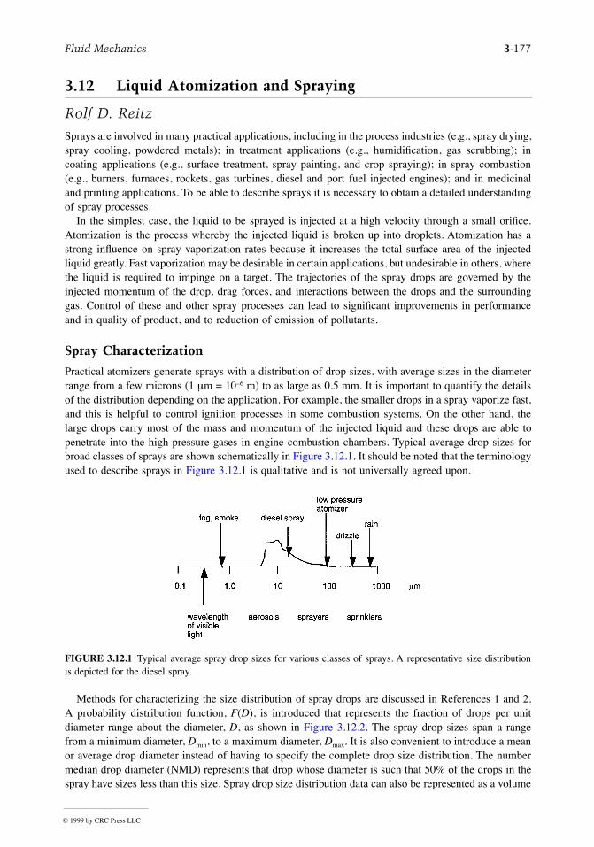
Fluid Mechanics 3-177
3.12 Liquid Atomization and Spraying
Rolf D. Reitz
Sprays are involved in many practical applications, including in the process industries (e.g., spray drying,spray cooling, powdered metals); in treatment applications (e.g., humidiÞcation, gas scrubbing); incoating applications (e.g., surface treatment, spray painting, and crop spraying); in spray combustion(e.g., burners, furnaces, rockets, gas turbines, diesel and port fuel injected engines); and in medicinaland printing applications. To be able to describe sprays it is necessary to obtain a detailed understandingof spray processes.
In the simplest case, the liquid to be sprayed is injected at a high velocity through a small oriÞce.Atomization is the process whereby the injected liquid is broken up into droplets. Atomization has astrong inßuence on spray vaporization rates because it increases the total surface area of the injectedliquid greatly. Fast vaporization may be desirable in certain applications, but undesirable in others, wherethe liquid is required to impinge on a target. The trajectories of the spray drops are governed by theinjected momentum of the drop, drag forces, and interactions between the drops and the surroundinggas. Control of these and other spray processes can lead to signiÞcant improvements in performanceand in quality of product, and to reduction of emission of pollutants.
Spray Characterization
Practical atomizers generate sprays with a distribution of drop sizes, with average sizes in the diameterrange from a few microns (1 mm = 10Ð6 m) to as large as 0.5 mm. It is important to quantify the detailsof the distribution depending on the application. For example, the smaller drops in a spray vaporize fast,and this is helpful to control ignition processes in some combustion systems. On the other hand, thelarge drops carry most of the mass and momentum of the injected liquid and these drops are able topenetrate into the high-pressure gases in engine combustion chambers. Typical average drop sizes forbroad classes of sprays are shown schematically in Figure 3.12.1. It should be noted that the terminologyused to describe sprays in Figure 3.12.1 is qualitative and is not universally agreed upon.
Methods for characterizing the size distribution of spray drops are discussed in References 1 and 2.A probability distribution function, F(D), is introduced that represents the fraction of drops per unitdiameter range about the diameter, D, as shown in Figure 3.12.2. The spray drop sizes span a rangefrom a minimum diameter, Dmin, to a maximum diameter, Dmax. It is also convenient to introduce a meanor average drop diameter instead of having to specify the complete drop size distribution. The numbermedian drop diameter (NMD) represents that drop whose diameter is such that 50% of the drops in thespray have sizes less than this size. Spray drop size distribution data can also be represented as a volume
FIGURE 3.12.1 Typical average spray drop sizes for various classes of sprays. A representative size distributionis depicted for the diesel spray.
© 1999 by CRC Press LLC
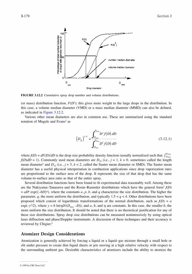
3-178 Section 3
(or mass) distribution function, F(D3); this gives more weight to the large drops in the distribution. Inthis case, a volume median diameter (VMD) or a mass median diameter (MMD) can also be deÞned,as indicated in Figure 3.12.2.
Various other mean diameters are also in common use. These are summarized using the standardnotation of Mugele and Evans2 as
(3.12.1)
where f(D) = dF(D)/dD is the drop size probability density function (usually normalized such that f(D)dD = 1). Commonly used mean diameters are D10 (i.e., j = 1, k = 0, sometimes called the lengthmean diameter3 and D32 (i.e., j = 3, k = 2, called the Sauter mean diameter or SMD). The Sauter meandiameter has a useful physical interpretation in combustion applications since drop vaporization ratesare proportional to the surface area of the drop. It represents the size of that drop that has the samevolume-to-surface area ratio as that of the entire spray.
Several distribution functions have been found to Þt experimental data reasonably well. Among theseare the NukiyamaÐTanasawa and the RosinÐRammler distributions which have the general form3 f(D)= aDp exp({ÐbD}q), where the constants a, p, b, and q characterize the size distribution. The higher theparameter, q, the more uniform the distribution, and typically 1.5 < q < 4. Other distributions have beenproposed which consist of logarithmic transformations of the normal distribution, such as f(D) = aexp(Ðy2/2), where y = d ln(hD/(Dmax ÐD)), and a, d, and h are constants. In this case, the smaller d, themore uniform the size distribution. It should be noted that there is no theoretical justiÞcation for any ofthese size distributions. Spray drop size distributions can be measured nonintrusively by using opticallaser diffraction and phase/Doppler instruments. A discussion of these techniques and their accuracy isreviewed by Chigier.4
Atomizer Design Considerations
Atomization is generally achieved by forcing a liquid or a liquidÐgas mixture through a small hole orslit under pressure to create thin liquid sheets or jets moving at a high relative velocity with respect tothe surrounding ambient gas. Desirable characteristics of atomizers include the ability to atomize the
FIGURE 3.12.2 Cumulative spray drop number and volume distributions.
D
D f D dD
D f D dDjk
j k D
Dj
D
Dk
( ) =( )
( )
- òò
min
max
min
max
ò DD
min
max
© 1999 by CRC Press LLC
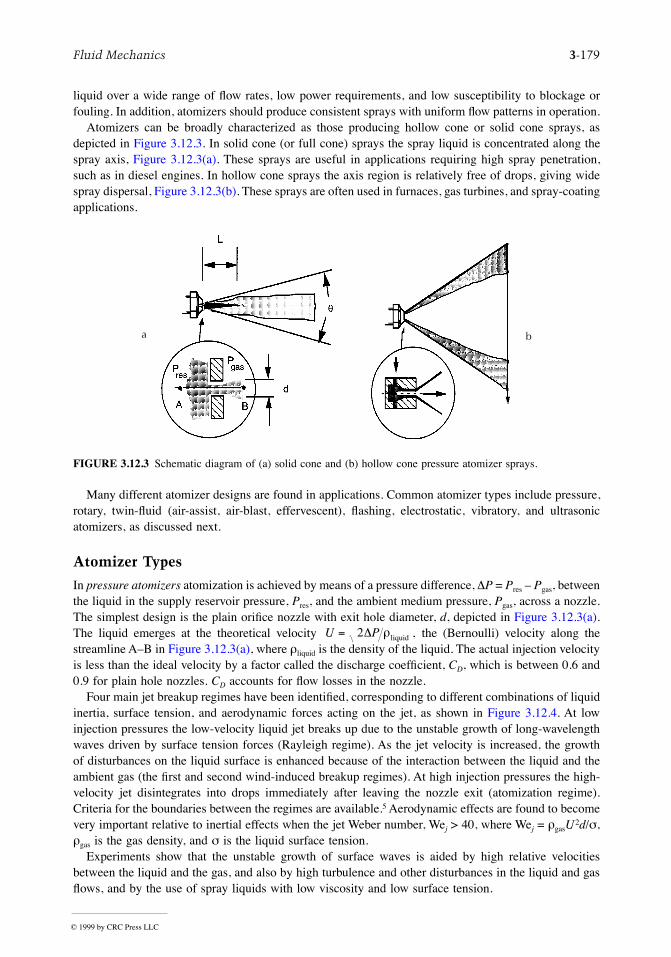
Fluid Mechanics 3-179
liquid over a wide range of ßow rates, low power requirements, and low susceptibility to blockage orfouling. In addition, atomizers should produce consistent sprays with uniform ßow patterns in operation.
Atomizers can be broadly characterized as those producing hollow cone or solid cone sprays, asdepicted in Figure 3.12.3. In solid cone (or full cone) sprays the spray liquid is concentrated along thespray axis, Figure 3.12.3(a). These sprays are useful in applications requiring high spray penetration,such as in diesel engines. In hollow cone sprays the axis region is relatively free of drops, giving widespray dispersal, Figure 3.12.3(b). These sprays are often used in furnaces, gas turbines, and spray-coatingapplications.
Many different atomizer designs are found in applications. Common atomizer types include pressure,rotary, twin-ßuid (air-assist, air-blast, effervescent), ßashing, electrostatic, vibratory, and ultrasonicatomizers, as discussed next.
Atomizer Types
In pressure atomizers atomization is achieved by means of a pressure difference, DP = Pres Ð Pgas, betweenthe liquid in the supply reservoir pressure, Pres, and the ambient medium pressure, Pgas, across a nozzle.The simplest design is the plain oriÞce nozzle with exit hole diameter, d, depicted in Figure 3.12.3(a).The liquid emerges at the theoretical velocity , the (Bernoulli) velocity along thestreamline AÐB in Figure 3.12.3(a), where rliquid is the density of the liquid. The actual injection velocityis less than the ideal velocity by a factor called the discharge coefÞcient, CD, which is between 0.6 and0.9 for plain hole nozzles. CD accounts for ßow losses in the nozzle.
Four main jet breakup regimes have been identiÞed, corresponding to different combinations of liquidinertia, surface tension, and aerodynamic forces acting on the jet, as shown in Figure 3.12.4. At lowinjection pressures the low-velocity liquid jet breaks up due to the unstable growth of long-wavelengthwaves driven by surface tension forces (Rayleigh regime). As the jet velocity is increased, the growthof disturbances on the liquid surface is enhanced because of the interaction between the liquid and theambient gas (the Þrst and second wind-induced breakup regimes). At high injection pressures the high-velocity jet disintegrates into drops immediately after leaving the nozzle exit (atomization regime).Criteria for the boundaries between the regimes are available.5 Aerodynamic effects are found to becomevery important relative to inertial effects when the jet Weber number, Wej > 40, where Wej = rgasU2d/s,rgas is the gas density, and s is the liquid surface tension.
Experiments show that the unstable growth of surface waves is aided by high relative velocitiesbetween the liquid and the gas, and also by high turbulence and other disturbances in the liquid and gasßows, and by the use of spray liquids with low viscosity and low surface tension.
a b
FIGURE 3.12.3 Schematic diagram of (a) solid cone and (b) hollow cone pressure atomizer sprays.
U = 2DP rliquid
© 1999 by CRC Press LLC
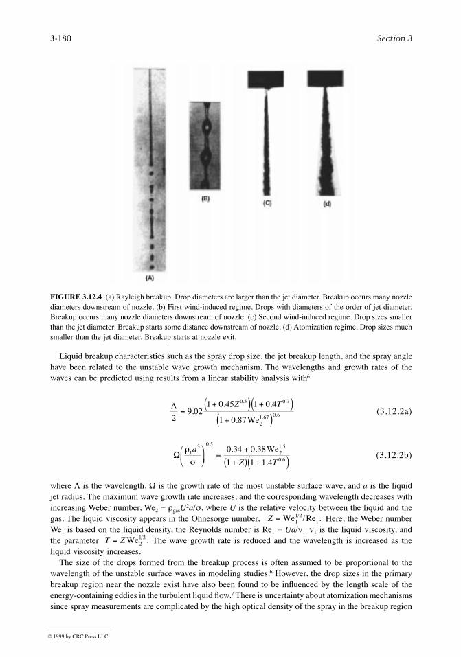
3-180 Section 3
Liquid breakup characteristics such as the spray drop size, the jet breakup length, and the spray anglehave been related to the unstable wave growth mechanism. The wavelengths and growth rates of thewaves can be predicted using results from a linear stability analysis with6
(3.12.2a)
(3.12.2b)
where L is the wavelength, W is the growth rate of the most unstable surface wave, and a is the liquidjet radius. The maximum wave growth rate increases, and the corresponding wavelength decreases withincreasing Weber number, We2 = rgasU2a/s, where U is the relative velocity between the liquid and thegas. The liquid viscosity appears in the Ohnesorge number, Here, the Weber numberWe1 is based on the liquid density, the Reynolds number is Re1 = Ua/n1, n1 is the liquid viscosity, andthe parameter The wave growth rate is reduced and the wavelength is increased as theliquid viscosity increases.
The size of the drops formed from the breakup process is often assumed to be proportional to thewavelength of the unstable surface waves in modeling studies.6 However, the drop sizes in the primarybreakup region near the nozzle exist have also been found to be inßuenced by the length scale of theenergy-containing eddies in the turbulent liquid ßow.7 There is uncertainty about atomization mechanismssince spray measurements are complicated by the high optical density of the spray in the breakup region
FIGURE 3.12.4 (a) Rayleigh breakup. Drop diameters are larger than the jet diameter. Breakup occurs many nozzlediameters downstream of nozzle. (b) First wind-induced regime. Drops with diameters of the order of jet diameter.Breakup occurs many nozzle diameters downstream of nozzle. (c) Second wind-induced regime. Drop sizes smallerthan the jet diameter. Breakup starts some distance downstream of nozzle. (d) Atomization regime. Drop sizes muchsmaller than the jet diameter. Breakup starts at nozzle exit.
L2
9 021 0 45 1 0 4
1 0 87
0 5 0 7
0 6=+( ) +( )
+( ).
. .
.
. .
.
Z T
We21.67
Wr
s1
3 0 5
0 6
0 34 0 38
1 1 1 4
a
Z T
æ
èç
ö
ø÷ =
+
+( ) +( )
.
.
. .
.
We21.5
Z = We Re11 2 / .1
T Z= We21 2 .
© 1999 by CRC Press LLC
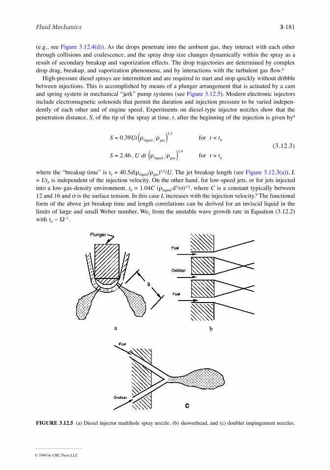
Fluid Mechanics 3-181
(e.g., see Figure 3.12.4(d)). As the drops penetrate into the ambient gas, they interact with each otherthrough collisions and coalescence, and the spray drop size changes dynamically within the spray as aresult of secondary breakup and vaporization effects. The drop trajectories are determined by complexdrop drag, breakup, and vaporization phenomena, and by interactions with the turbulent gas ßow.6
High-pressure diesel sprays are intermittent and are required to start and stop quickly without dribblebetween injections. This is accomplished by means of a plunger arrangement that is actuated by a camand spring system in mechanical ÒjerkÓ pump systems (see Figure 3.12.5). Modern electronic injectorsinclude electromagnetic solenoids that permit the duration and injection pressure to be varied indepen-dently of each other and of engine speed. Experiments on diesel-type injector nozzles show that thepenetration distance, S, of the tip of the spray at time, t, after the beginning of the injection is given by8
(3.12.3)
where the Òbreakup timeÓ is tb = 40.5d(rliquid/rgas)1/2/U. The jet breakup length (see Figure 3.12.3(a)), L= Utb is independent of the injection velocity. On the other hand, for low-speed jets, or for jets injectedinto a low-gas-density environment, tb = 1.04C (rliquid d3/s)1/2, where C is a constant typically between12 and 16 and s is the surface tension. In this case L increases with the injection velocity.9 The functionalform of the above jet breakup time and length correlations can be derived for an inviscid liquid in thelimits of large and small Weber number, We2 from the unstable wave growth rate in Equation (3.12.2)with tb ~ WÐ1.
FIGURE 3.12.5 (a) Diesel injector multihole spray nozzle, (b) showerhead, and (c) doublet impingement nozzles.
S Ut t t
S U dt t t
b
b
= ( ) <
= ( ) >
0 39
2 46
1 2
1 4
.
.
r r
r r
liquid gas
liquid gas
for
for
© 1999 by CRC Press LLC
3-182 Section 3
For high-speed diesel-type jets in the atomization regime the resulting spray diverges in the form ofa cone with cone angle, q, that is usually in the range from 5 to 20°. q increases with gas densityfollowing tan q = A(rgas/rliquid)1/2, where A is a constant that depends on the nozzle passage length and(weakly) on the injection velocity.9 Very high injection pressures are required to produce small drops.In diesel engines DP is typically as high as 200 Mpa, and drops are produced with mean diameters ofthe order of 10 mm (see Figure 3.12.1). Drop size correlations have been proposed for plain-oriÞcesprays, such as that presented in Table 3.12.1.3 Note, however, that these correlations do not account forthe fact that the spray drop size varies with time, and from place to place in the spray. Moreover,experimental correlations often do not include some parameters that are known to inßuence spray dropsizes, such as the nozzle passage length and its entrance geometry. Therefore, overall drop size corre-lations should only be used with caution.
The plain oriÞce design is also used in twin-ßuid-type liquid rocket engines in showerhead and doubletdesigns (Figures 3.12.5b and 3.12.5c). In the case of doublet nozzles, shown in Figure 3.12.6c, theimpinging jets create unstable liquid sheets which break up to produce the sprays. Drop size correlationsare available for liquid sheets such as those formed by discharging the liquid through a rectangular slit(see fan spray, Table 3.12.1). Thin liquid sheets or slits lead to the production of small drops. Thebreakup mechanism of liquid sheets is also thought to involve the unstable growth of surface waves dueto surface tension and aerodynamic forces.5
In rotary atomizers centrifugal forces are used to further enhance the breakup process. In this casethe liquid is supplied to the center of a spinning disk and liquid sheets or ligaments are thrown off theedges of the disk. The drop size depends on the rotational speed of the disk, as indicated in Table 3.12.1.
TABLE 3.12.1 Representative Drop Size Correlations for Various Spray Devices (Dimensional quantities are in SI units, kg, m, s)
Device Correlation Notes
Plain oriÞce Use SI units
Fan spray dh = nozzle hydraulic diameter
Rotary atomizer
N = rotational speed (rev/sec), Q = volumetric ßow rate, Ainj U
Pressure swirl
t = Þlm thickness; q = cone angle, d = discharge oriÞce diameter
Twin ßuid/air blast
ALR = air-to-liquid mass ratio
PreÞlming air blast
dh = hydraulic diameter, dp = preÞlmer diameter, Figure 3.12.9
Ultrasonic w = vibration frequency
Source: Lefebvre, A.H., Atomization and Sprays, Hemisphere Publishing, New York, 1989. With permission.
SMD liquid gas= ( ) -3 08 10 385
0 7370 06 0 54. .
.. .n r s r DP
SMD liquid2
gas
liquid gas
= ( )
+ ( )
2 83
0 26
3 20 25
0 25
.
.
.
.
d d P
d d P
h h
h h
sm r
sr r
D
D
SMD liquid liquid0.1= 0 119 0 1 0 5 0 5 0 4
. . . . .
Q Nds r m
SMD liquid2
gas
liquid gas
inj liquid
= ( ) ( )
+ ( ) ( )
=
4 52
0 39
0 0114
20 25 0 25
0 25 0 75
1 2
. cos
. cos
. cos
. .
. .
sm r q
sr r q
r q
D
D
P t
P t
t A d
SMD ALR
ALR
gas
liquid2
liquid
= ( ) +( )
+ ( ) +( )
0 48 1 1
0 15 1 1
20 4 0 4
0 5
.
.
. .
.
d U d
d d
s r
m sr
SMD ALR gas
liquid2
liquid
= +( ) ( )éëê
+ ( ) ùûú
1 1 0 33
0 068
20 6
0 5
.
.
.
.
d U d
d d
h p
h p
s r
m sr
SMD liquid= ( )4 3 21 3
p s r w
© 1999 by CRC Press LLC
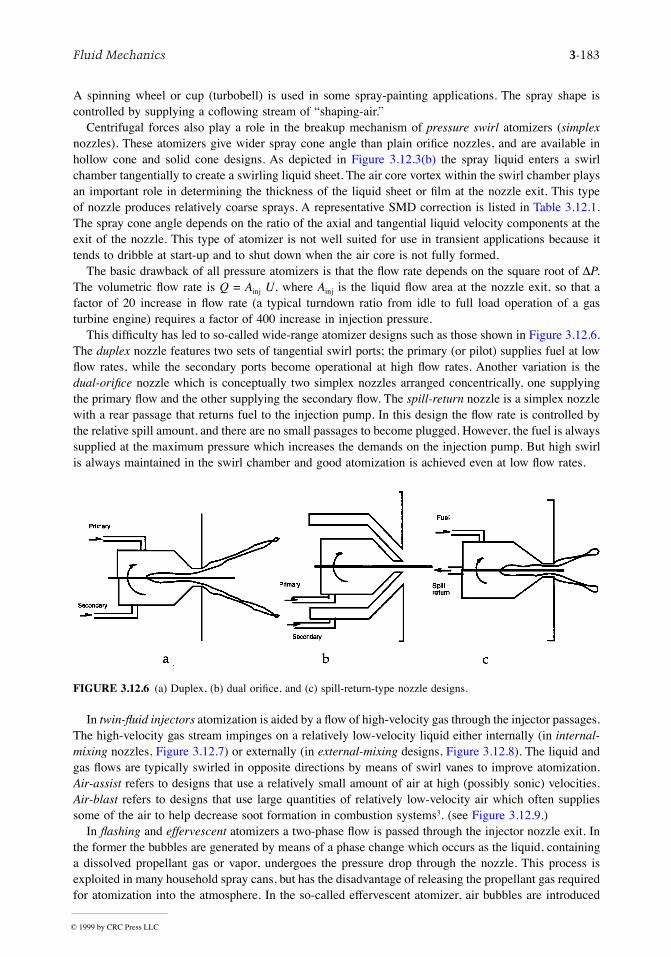
Fluid Mechanics 3-183
A spinning wheel or cup (turbobell) is used in some spray-painting applications. The spray shape iscontrolled by supplying a coßowing stream of Òshaping-air.Ó
Centrifugal forces also play a role in the breakup mechanism of pressure swirl atomizers (simplexnozzles). These atomizers give wider spray cone angle than plain oriÞce nozzles, and are available inhollow cone and solid cone designs. As depicted in Figure 3.12.3(b) the spray liquid enters a swirlchamber tangentially to create a swirling liquid sheet. The air core vortex within the swirl chamber playsan important role in determining the thickness of the liquid sheet or Þlm at the nozzle exit. This typeof nozzle produces relatively coarse sprays. A representative SMD correction is listed in Table 3.12.1.The spray cone angle depends on the ratio of the axial and tangential liquid velocity components at theexit of the nozzle. This type of atomizer is not well suited for use in transient applications because ittends to dribble at start-up and to shut down when the air core is not fully formed.
The basic drawback of all pressure atomizers is that the ßow rate depends on the square root of DP.The volumetric ßow rate is Q = Ainj U, where Ainj is the liquid ßow area at the nozzle exit, so that afactor of 20 increase in ßow rate (a typical turndown ratio from idle to full load operation of a gasturbine engine) requires a factor of 400 increase in injection pressure.
This difÞculty has led to so-called wide-range atomizer designs such as those shown in Figure 3.12.6.The duplex nozzle features two sets of tangential swirl ports; the primary (or pilot) supplies fuel at lowßow rates, while the secondary ports become operational at high ßow rates. Another variation is thedual-oriÞce nozzle which is conceptually two simplex nozzles arranged concentrically, one supplyingthe primary ßow and the other supplying the secondary ßow. The spill-return nozzle is a simplex nozzlewith a rear passage that returns fuel to the injection pump. In this design the ßow rate is controlled bythe relative spill amount, and there are no small passages to become plugged. However, the fuel is alwayssupplied at the maximum pressure which increases the demands on the injection pump. But high swirlis always maintained in the swirl chamber and good atomization is achieved even at low ßow rates.
In twin-ßuid injectors atomization is aided by a ßow of high-velocity gas through the injector passages.The high-velocity gas stream impinges on a relatively low-velocity liquid either internally (in internal-mixing nozzles, Figure 3.12.7) or externally (in external-mixing designs, Figure 3.12.8). The liquid andgas ßows are typically swirled in opposite directions by means of swirl vanes to improve atomization.Air-assist refers to designs that use a relatively small amount of air at high (possibly sonic) velocities.Air-blast refers to designs that use large quantities of relatively low-velocity air which often suppliessome of the air to help decrease soot formation in combustion systems3. (see Figure 3.12.9.)
In ßashing and effervescent atomizers a two-phase ßow is passed through the injector nozzle exit. Inthe former the bubbles are generated by means of a phase change which occurs as the liquid, containinga dissolved propellant gas or vapor, undergoes the pressure drop through the nozzle. This process isexploited in many household spray cans, but has the disadvantage of releasing the propellant gas requiredfor atomization into the atmosphere. In the so-called effervescent atomizer, air bubbles are introduced
FIGURE 3.12.6 (a) Duplex, (b) dual oriÞce, and (c) spill-return-type nozzle designs.
© 1999 by CRC Press LLC
3-184 Section 3
into the liquid upstream of the exit oriÞce, as depicted in Figure 3.12.10. The spray quality is found todepend weakly on the air bubble size and is independent of the nozzle exit diameter. This makes internal-mixing, air-assist atomizers very attractive for use with high-viscosity ßuids and slurries where nozzleplugging would otherwise be a problem.3
In electrostatic atomizers the spray liquid is charged by applying a high-voltage drop across the nozzle.The dispersion of the spray drops is increased by exploiting electrical repulsive forces between thedroplets. An electrostatic charge on the drops is also helpful in spray-coating applications, such as inautomotive spray painting using electrostatic turbobell sprayers, since the charged drops are attracted toan oppositely charged target surface.
Other atomizer types include vibratory and ultrasonic atomizers (or nebulizers), where the drops areformed by vibrating the injector nozzle at high frequencies and at large amplitudes to produce short-wavelength disturbances to the liquid ßow. Ultrasonic atomizers are used in inhalation therapy wherevery Þne sprays (submicron sizes) are required, and an available representative drop size correlation isalso listed in Table 3.12.1.
FIGURE 3.12.7 Internal-mixing twin-ßuid injectordesign.
FIGURE 3.12.8 External-mixing twin-ßuid injectordesign.
FIGURE 3.12.9 PreÞlming air blast atomizer. FIGURE 3.12.10 Internal-mixing, effervescentatomizer.
© 1999 by CRC Press LLC
Fluid Mechanics 3-185
References
1. American Society for Testing and Materials (ASTM) Standard E799. 1988. Data Criteria andProcessing for Liquid Drop Size Analysis.
2. Mugele, R. and Evans, H.D. 1951. Droplet size distributions in sprays, Ind. Eng. Chem., 43,1317Ð1324.
3. Lefebvre, A.H. 1989. Atomization and Sprays, Hemisphere Publishing, New York.4. Chigier, N.A. 1983. Drop size and velocity instrumentation, Prog. Energ. Combust. Sci., 9,
155Ð177.5. Chigier, N. and Reitz, R.D. 1996. Regimes of jet breakup, in Progress in Astronautics and
Aeronautics Series, K. Kuo, Ed., AIAA, New York, Chapter 4, pp. 109Ð135.6. Reitz, R.D. 1988. Modeling atomization processes in high-pressure vaporizing sprays, Atomisation
Spray Technol., 3, 309Ð337.7. Wu, P-K., Miranda, R.F., and Faeth, G.M. 1995. Effects of initial ßow conditions on primary
breakup of nonturbulent and turbulent round liquid jets, Atomization Sprays, 5, 175Ð196.8. Hiroyasu, H. and Arai, M. 1978. Fuel spray penetration and spray angle in diesel engines, Trans.
JSAE, 34, 3208.9. Reitz, R.D. and Bracco, F.V. 1986. Mechanisms of breakup of round liquid jets, in The Encyclo-
pedia of Fluid Mechanics, Vol. 3, N. Cheremisnoff, Ed., Gulf Publishing, Houston, TX, Chapter10, 233Ð249.
Further Information
Information about recent work in the Þeld of atomization and sprays can be obtained through participationin the Institutes for Liquid Atomization and Spraying Systems (ILASS-Americas, -Europe, -Japan, -Korea). These regional ILASS sections hold annual meetings. An international congress (ICLASS) isalso held biennially. More information is available on the ILASS-Americas homepage athttp://ucicl.eng.uci.edu/ilass. AfÞliated with the ILASS organizations is the InstituteÕs Journal publicationAtomization and Sprays published by Begell House, Inc., New York.
© 1999 by CRC Press LLC
3-186 Section 3
3.13 Flow Measurement*
Alan T. McDonald and Sherif A. Sherif
This section deals with the measurement of mass ßow rate or volume ßow rate of a ßuid in an enclosedpipe or duct system. Flow measurement in open channels is treated in Section 3.10 of this book.
The choice of a ßow meter type and size depends on the required accuracy, range, cost, ease of readingor data reduction, and service life. Always select the simplest and cheapest device that gives the desiredaccuracy.
Direct Methods
Tanks can be used to determine the ßow rate for steady liquid ßows by measuring the volume or massof liquid collected during a known time interval. If the time interval is long enough, ßow rates may bedetermined precisely using tanks. Compressibility must be considered in gas volume measurements. Itis not practical to measure the mass of gas, but a volume sample can be collected by placing an invertedÒbellÓ over water and holding the pressure constant by counterweights. No calibration is required whenvolume measurements are set up carefully; this is a great advantage of direct methods.
Positive-displacement ßow meters may be used in specialized applications, particularly for remoteor recording uses. For example, household water and natural gas meters are calibrated to read directlyin units of product. Gasoline metering pumps measure total ßow and automatically compute the cost.Many positive-displacement meters are available commercially. Consult manufacturersÕ literature orReference 7 for design and installation details.
Restriction Flow Meters for Flow in Ducts
Most restriction ßow meters for internal ßow (except the laminar ßow element) are based on accelerationof a ßuid stream through some form of nozzle, shown schematically in Figure 3.13.1. Flow separatingfrom the sharp edge of the nozzle throat forms a recirculation zone shown by the dashed lines downstreamfrom the nozzle. The main ßow stream continues to accelerate from the nozzle throat to form a venacontracta at section (2) and then decelerates again to Þll the duct. At the vena contracta, the ßow areais a minimum, the ßow streamlines are essentially straight, and the pressure is uniform across the channelsection. The theoretical ßow rate is
(3.13.1)
Equation (3.13.1) shows the general relationship for a restriction ßow meter: Mass ßow rate isproportional to the square root of the pressure differential across the meter taps. This relationship limitsthe ßow rates that can be measured accurately to approximately a 4:1 range.
Several factors limit the utility of Equation (3.13.1) for calculating the actual mass ßow rate througha meter. The actual ßow area at section (2) is unknown when the vena contracta is pronounced (e.g.,for oriÞce plates when Dt is a small fraction of D1). The velocity proÞles approach uniform ßow onlyat large Reynolds number. Frictional effects can become important (especially downstream from themeter) when the meter contours are abrupt. Finally, the location of the pressure taps inßuences thedifferential pressure reading, p1 Ð p2.
The actual mass ßow rate is given by
* The contributors of this chapter were asked to conform as much as possible to the nomenclature presentedbelow, but deÞne new terms pertaining to their particular area of specialty in the context of the chapter.
ÇmA
A Ap ptheoretical =
- ( )-( )2
2 1
2 1 2
12r
© 1999 by CRC Press LLC
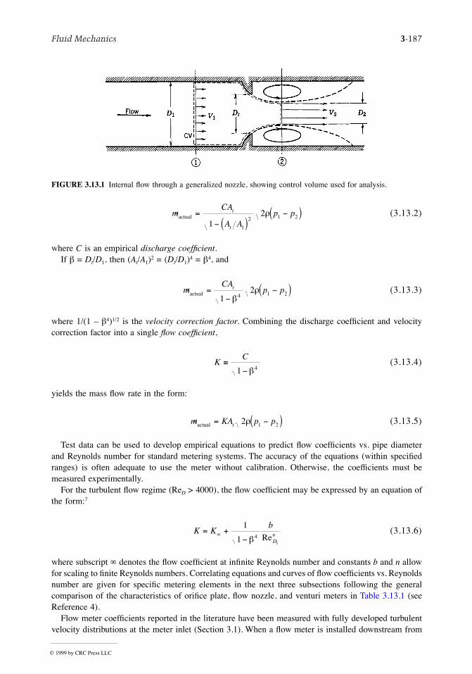
Fluid Mechanics 3-187
(3.13.2)
where C is an empirical discharge coefÞcient.If b = Dt/D1, then (At/A1)2 = (Dt/D1)4 = b4, and
(3.13.3)
where 1/(1 Ð b4)1/2 is the velocity correction factor. Combining the discharge coefÞcient and velocitycorrection factor into a single ßow coefÞcient,
(3.13.4)
yields the mass ßow rate in the form:
(3.13.5)
Test data can be used to develop empirical equations to predict ßow coefÞcients vs. pipe diameterand Reynolds number for standard metering systems. The accuracy of the equations (within speciÞedranges) is often adequate to use the meter without calibration. Otherwise, the coefÞcients must bemeasured experimentally.
For the turbulent ßow regime (ReD > 4000), the ßow coefÞcient may be expressed by an equation ofthe form:7
(3.13.6)
where subscript ¥ denotes the ßow coefÞcient at inÞnite Reynolds number and constants b and n allowfor scaling to Þnite Reynolds numbers. Correlating equations and curves of ßow coefÞcients vs. Reynoldsnumber are given for speciÞc metering elements in the next three subsections following the generalcomparison of the characteristics of oriÞce plate, ßow nozzle, and venturi meters in Table 3.13.1 (seeReference 4).
Flow meter coefÞcients reported in the literature have been measured with fully developed turbulentvelocity distributions at the meter inlet (Section 3.1). When a ßow meter is installed downstream from
FIGURE 3.13.1 Internal ßow through a generalized nozzle, showing control volume used for analysis.
ÇmCA
A Ap pt
t
actual =- ( )
-( )1
2
1
2 1 2r
ÇmCA
p ptactual =
--( )
12
4 1 2b
r
KC
º-1 4b
Çm KA p ptactual = -( )2 1 2r
K Kb
Dn= +
-¥
1
1 41
b Re
© 1999 by CRC Press LLC
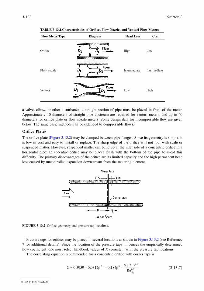
3-188 Section 3
a valve, elbow, or other disturbance, a straight section of pipe must be placed in front of the meter.Approximately 10 diameters of straight pipe upstream are required for venturi meters, and up to 40diameters for oriÞce plate or ßow nozzle meters. Some design data for incompressible ßow are givenbelow. The same basic methods can be extended to compressible ßows.7
Orifice Plates
The oriÞce plate (Figure 3.13.2) may be clamped between pipe ßanges. Since its geometry is simple, itis low in cost and easy to install or replace. The sharp edge of the oriÞce will not foul with scale orsuspended matter. However, suspended matter can build up at the inlet side of a concentric oriÞce in ahorizontal pipe; an eccentric oriÞce may be placed ßush with the bottom of the pipe to avoid thisdifÞculty. The primary disadvantages of the oriÞce are its limited capacity and the high permanent headloss caused by uncontrolled expansion downstream from the metering element.
Pressure taps for oriÞces may be placed in several locations as shown in Figure 3.13.2 (see Reference7 for additional details). Since the location of the pressure taps inßuences the empirically determinedßow coefÞcient, one must select handbook values of K consistent with the pressure tap locations.
The correlating equation recommended for a concentric oriÞce with corner taps is
(3.13.7)
TABLE 3.13.1.Characteristics of OriÞce, Flow Nozzle, and Venturi Flow Meters
Flow Meter Type Diagram Head Loss Cost
OriÞce High Low
Flow nozzle Intermediate Intermediate
Venturi Low High
FIGURE 3.13.2 OriÞce geometry and pressure tap locations.
CD
= + - +0 5959 0 0312 0 18491 712 1 8
2 5
0 75
1
. . ...
.
.b bb
Re
© 1999 by CRC Press LLC
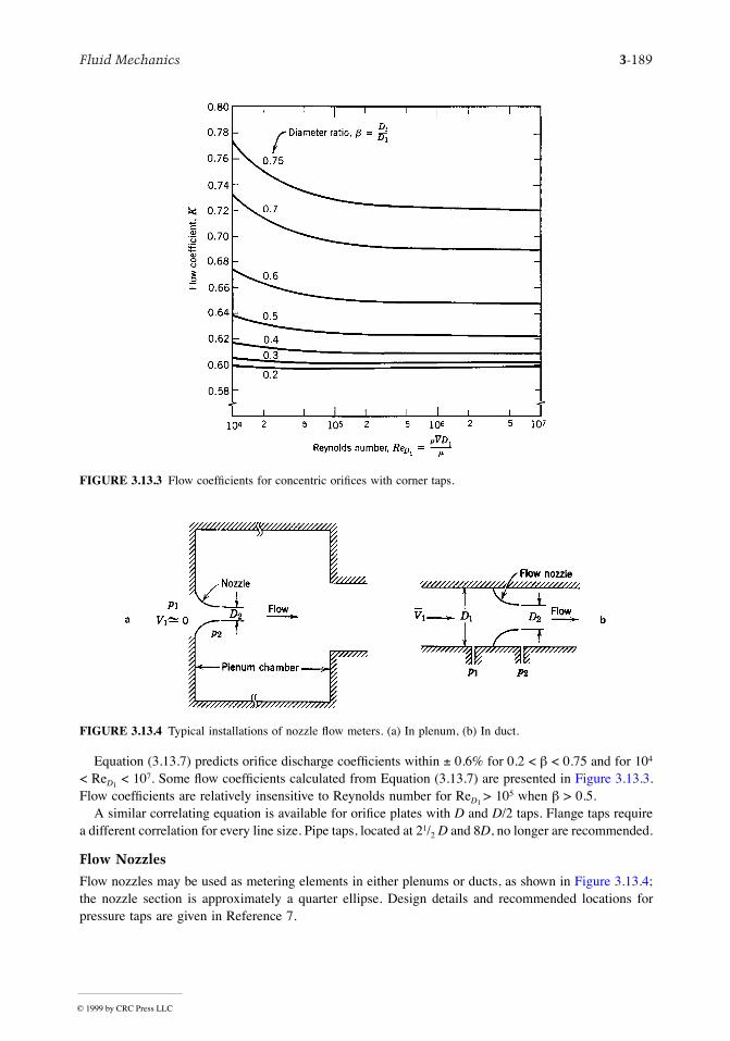
Fluid Mechanics 3-189
Equation (3.13.7) predicts oriÞce discharge coefÞcients within ± 0.6% for 0.2 < b < 0.75 and for 104
< ReD1 < 107. Some ßow coefÞcients calculated from Equation (3.13.7) are presented in Figure 3.13.3.
Flow coefÞcients are relatively insensitive to Reynolds number for ReD1 > 105 when b > 0.5.A similar correlating equation is available for oriÞce plates with D and D/2 taps. Flange taps require
a different correlation for every line size. Pipe taps, located at 21/2 D and 8D, no longer are recommended.
Flow Nozzles
Flow nozzles may be used as metering elements in either plenums or ducts, as shown in Figure 3.13.4;the nozzle section is approximately a quarter ellipse. Design details and recommended locations forpressure taps are given in Reference 7.
FIGURE 3.13.3 Flow coefÞcients for concentric oriÞces with corner taps.
FIGURE 3.13.4 Typical installations of nozzle ßow meters. (a) In plenum, (b) In duct.
© 1999 by CRC Press LLC
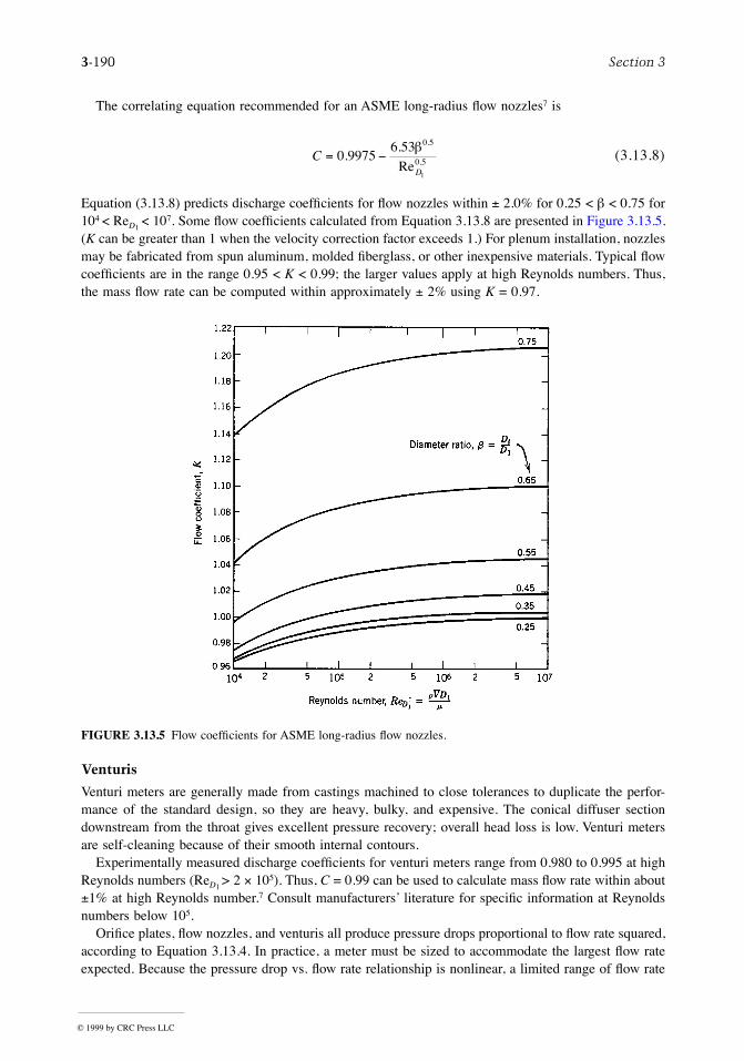
3-190 Section 3
The correlating equation recommended for an ASME long-radius ßow nozzles7 is
(3.13.8)
Equation (3.13.8) predicts discharge coefÞcients for ßow nozzles within ± 2.0% for 0.25 < b < 0.75 for104 < ReD1 < 107. Some ßow coefÞcients calculated from Equation 3.13.8 are presented in Figure 3.13.5.(K can be greater than 1 when the velocity correction factor exceeds 1.) For plenum installation, nozzlesmay be fabricated from spun aluminum, molded Þberglass, or other inexpensive materials. Typical ßowcoefÞcients are in the range 0.95 < K < 0.99; the larger values apply at high Reynolds numbers. Thus,the mass ßow rate can be computed within approximately ± 2% using K = 0.97.
Venturis
Venturi meters are generally made from castings machined to close tolerances to duplicate the perfor-mance of the standard design, so they are heavy, bulky, and expensive. The conical diffuser sectiondownstream from the throat gives excellent pressure recovery; overall head loss is low. Venturi metersare self-cleaning because of their smooth internal contours.
Experimentally measured discharge coefÞcients for venturi meters range from 0.980 to 0.995 at highReynolds numbers (ReD1 > 2 ´ 105). Thus, C = 0.99 can be used to calculate mass ßow rate within about±1% at high Reynolds number.7 Consult manufacturersÕ literature for speciÞc information at Reynoldsnumbers below 105.
OriÞce plates, ßow nozzles, and venturis all produce pressure drops proportional to ßow rate squared,according to Equation 3.13.4. In practice, a meter must be sized to accommodate the largest ßow rateexpected. Because the pressure drop vs. ßow rate relationship is nonlinear, a limited range of ßow rate
FIGURE 3.13.5 Flow coefÞcients for ASME long-radius ßow nozzles.
CD
= -0 99756 53 0 5
0 5
1
.. .
.
bRe
© 1999 by CRC Press LLC
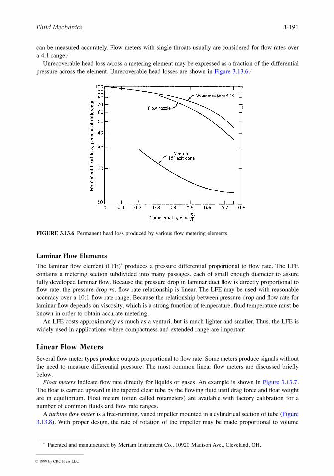
Fluid Mechanics 3-191
can be measured accurately. Flow meters with single throats usually are considered for ßow rates overa 4:1 range.7
Unrecoverable head loss across a metering element may be expressed as a fraction of the differentialpressure across the element. Unrecoverable head losses are shown in Figure 3.13.6.7
Laminar Flow Elements
The laminar ßow element (LFE)* produces a pressure differential proportional to ßow rate. The LFEcontains a metering section subdivided into many passages, each of small enough diameter to assurefully developed laminar ßow. Because the pressure drop in laminar duct ßow is directly proportional toßow rate, the pressure drop vs. ßow rate relationship is linear. The LFE may be used with reasonableaccuracy over a 10:1 ßow rate range. Because the relationship between pressure drop and ßow rate forlaminar ßow depends on viscosity, which is a strong function of temperature, ßuid temperature must beknown in order to obtain accurate metering.
An LFE costs approximately as much as a venturi, but is much lighter and smaller. Thus, the LFE iswidely used in applications where compactness and extended range are important.
Linear Flow Meters
Several ßow meter types produce outputs proportional to ßow rate. Some meters produce signals withoutthe need to measure differential pressure. The most common linear ßow meters are discussed brießybelow.
Float meters indicate ßow rate directly for liquids or gases. An example is shown in Figure 3.13.7.The ßoat is carried upward in the tapered clear tube by the ßowing ßuid until drag force and ßoat weightare in equilibrium. Float meters (often called rotameters) are available with factory calibration for anumber of common ßuids and ßow rate ranges.
A turbine ßow meter is a free-running, vaned impeller mounted in a cylindrical section of tube (Figure3.13.8). With proper design, the rate of rotation of the impeller may be made proportional to volume
* Patented and manufactured by Meriam Instrument Co., 10920 Madison Ave., Cleveland, OH.
FIGURE 3.13.6 Permanent head loss produced by various ßow metering elements.
© 1999 by CRC Press LLC
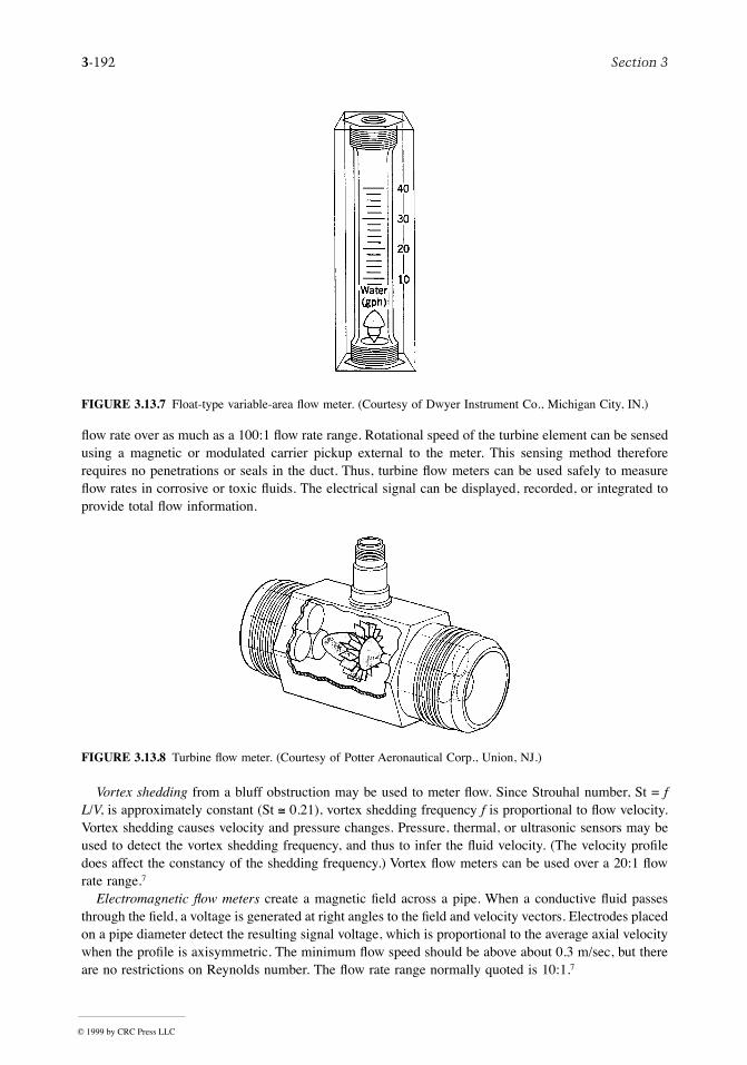
3-192 Section 3
ßow rate over as much as a 100:1 ßow rate range. Rotational speed of the turbine element can be sensedusing a magnetic or modulated carrier pickup external to the meter. This sensing method thereforerequires no penetrations or seals in the duct. Thus, turbine ßow meters can be used safely to measureßow rates in corrosive or toxic ßuids. The electrical signal can be displayed, recorded, or integrated toprovide total ßow information.
Vortex shedding from a bluff obstruction may be used to meter ßow. Since Strouhal number, St = fL/V, is approximately constant (St @ 0.21), vortex shedding frequency f is proportional to ßow velocity.Vortex shedding causes velocity and pressure changes. Pressure, thermal, or ultrasonic sensors may beused to detect the vortex shedding frequency, and thus to infer the ßuid velocity. (The velocity proÞledoes affect the constancy of the shedding frequency.) Vortex ßow meters can be used over a 20:1 ßowrate range.7
Electromagnetic ßow meters create a magnetic Þeld across a pipe. When a conductive ßuid passesthrough the Þeld, a voltage is generated at right angles to the Þeld and velocity vectors. Electrodes placedon a pipe diameter detect the resulting signal voltage, which is proportional to the average axial velocitywhen the proÞle is axisymmetric. The minimum ßow speed should be above about 0.3 m/sec, but thereare no restrictions on Reynolds number. The ßow rate range normally quoted is 10:1.7
FIGURE 3.13.7 Float-type variable-area ßow meter. (Courtesy of Dwyer Instrument Co., Michigan City, IN.)
FIGURE 3.13.8 Turbine ßow meter. (Courtesy of Potter Aeronautical Corp., Union, NJ.)
© 1999 by CRC Press LLC
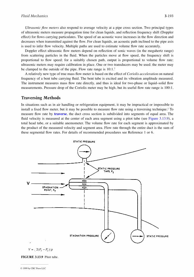
Fluid Mechanics 3-193
Ultrasonic ßow meters also respond to average velocity at a pipe cross section. Two principal typesof ultrasonic meters measure propagation time for clean liquids, and reßection frequency shift (Dopplereffect) for ßows carrying particulates. The speed of an acoustic wave increases in the ßow direction anddecreases when transmitted against the ßow. For clean liquids, an acoustic path inclined to the pipe axisis used to infer ßow velocity. Multiple paths are used to estimate volume ßow rate accurately.
Doppler effect ultrasonic ßow meters depend on reßection of sonic waves (in the megahertz range)from scattering particles in the ßuid. When the particles move at ßow speed, the frequency shift isproportional to ßow speed; for a suitably chosen path, output is proportional to volume ßow rate;ultrasonic meters may require calibration in place. One or two transducers may be used; the meter maybe clamped to the outside of the pipe. Flow rate range is 10:1.7
A relatively new type of true mass ßow meter is based on the effect of Coriolis acceleration on naturalfrequency of a bent tube carrying ßuid. The bent tube is excited and its vibration amplitude measured.The instrument measures mass ßow rate directly, and thus is ideal for two-phase or liquidÐsolid ßowmeasurements. Pressure drop of the Coriolis meter may be high, but its useful ßow rate range is 100:1.
Traversing Methods
In situations such as in air handling or refrigeration equipment, it may be impractical or impossible toinstall a Þxed ßow meter, but it may be possible to measure ßow rate using a traversing technique.1 Tomeasure ßow rate by traverse, the duct cross section is subdivided into segments of equal area. Theßuid velocity is measured at the center of each area segment using a pitot tube (see Figure 3.13.9), atotal head tube, or a suitable anemometer. The volume ßow rate for each segment is approximated bythe product of the measured velocity and segment area. Flow rate through the entire duct is the sum ofthese segmental ßow rates. For details of recommended procedures see Reference 1 or 6.
FIGURE 3.13.9 Pitot tube.
V P PT S= -2( ) r
© 1999 by CRC Press LLC
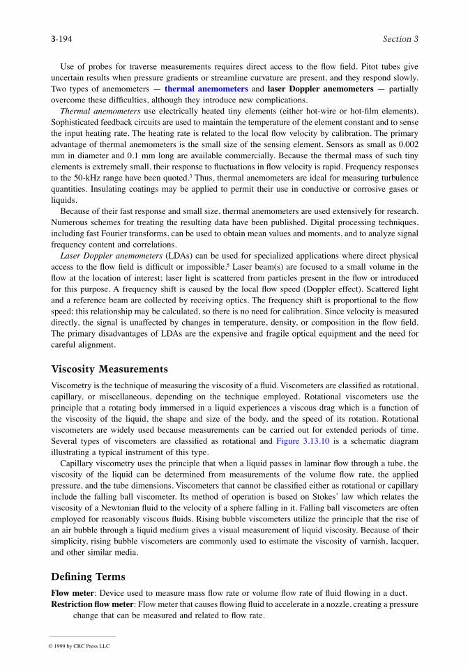
3-194 Section 3
Use of probes for traverse measurements requires direct access to the ßow Þeld. Pitot tubes giveuncertain results when pressure gradients or streamline curvature are present, and they respond slowly.Two types of anemometers Ñ thermal anemometers and laser Doppler anemometers Ñ partiallyovercome these difÞculties, although they introduce new complications.
Thermal anemometers use electrically heated tiny elements (either hot-wire or hot-Þlm elements).Sophisticated feedback circuits are used to maintain the temperature of the element constant and to sensethe input heating rate. The heating rate is related to the local ßow velocity by calibration. The primaryadvantage of thermal anemometers is the small size of the sensing element. Sensors as small as 0.002mm in diameter and 0.1 mm long are available commercially. Because the thermal mass of such tinyelements is extremely small, their response to ßuctuations in ßow velocity is rapid. Frequency responsesto the 50-kHz range have been quoted.3 Thus, thermal anemometers are ideal for measuring turbulencequantities. Insulating coatings may be applied to permit their use in conductive or corrosive gases orliquids.
Because of their fast response and small size, thermal anemometers are used extensively for research.Numerous schemes for treating the resulting data have been published. Digital processing techniques,including fast Fourier transforms, can be used to obtain mean values and moments, and to analyze signalfrequency content and correlations.
Laser Doppler anemometers (LDAs) can be used for specialized applications where direct physicalaccess to the ßow Þeld is difÞcult or impossible.5 Laser beam(s) are focused to a small volume in theßow at the location of interest; laser light is scattered from particles present in the ßow or introducedfor this purpose. A frequency shift is caused by the local ßow speed (Doppler effect). Scattered lightand a reference beam are collected by receiving optics. The frequency shift is proportional to the ßowspeed; this relationship may be calculated, so there is no need for calibration. Since velocity is measureddirectly, the signal is unaffected by changes in temperature, density, or composition in the ßow Þeld.The primary disadvantages of LDAs are the expensive and fragile optical equipment and the need forcareful alignment.
Viscosity Measurements
Viscometry is the technique of measuring the viscosity of a ßuid. Viscometers are classiÞed as rotational,capillary, or miscellaneous, depending on the technique employed. Rotational viscometers use theprinciple that a rotating body immersed in a liquid experiences a viscous drag which is a function ofthe viscosity of the liquid, the shape and size of the body, and the speed of its rotation. Rotationalviscometers are widely used because measurements can be carried out for extended periods of time.Several types of viscometers are classiÞed as rotational and Figure 3.13.10 is a schematic diagramillustrating a typical instrument of this type.
Capillary viscometry uses the principle that when a liquid passes in laminar ßow through a tube, theviscosity of the liquid can be determined from measurements of the volume ßow rate, the appliedpressure, and the tube dimensions. Viscometers that cannot be classiÞed either as rotational or capillaryinclude the falling ball viscometer. Its method of operation is based on StokesÕ law which relates theviscosity of a Newtonian ßuid to the velocity of a sphere falling in it. Falling ball viscometers are oftenemployed for reasonably viscous ßuids. Rising bubble viscometers utilize the principle that the rise ofan air bubble through a liquid medium gives a visual measurement of liquid viscosity. Because of theirsimplicity, rising bubble viscometers are commonly used to estimate the viscosity of varnish, lacquer,and other similar media.
Defining Terms
Flow meter: Device used to measure mass ßow rate or volume ßow rate of ßuid ßowing in a duct.Restriction ßow meter: Flow meter that causes ßowing ßuid to accelerate in a nozzle, creating a pressure
change that can be measured and related to ßow rate.
© 1999 by CRC Press LLC
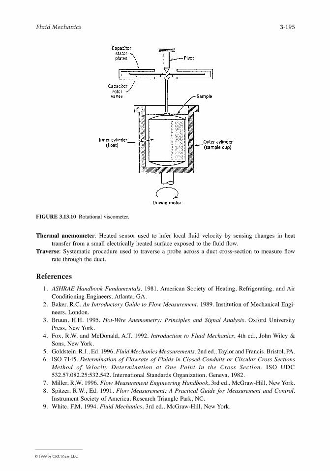
Fluid Mechanics 3-195
Thermal anemometer: Heated sensor used to infer local ßuid velocity by sensing changes in heattransfer from a small electrically heated surface exposed to the ßuid ßow.
Traverse: Systematic procedure used to traverse a probe across a duct cross-section to measure ßowrate through the duct.
References
1. ASHRAE Handbook Fundamentals. 1981. American Society of Heating, Refrigerating, and AirConditioning Engineers, Atlanta, GA.
2. Baker, R.C. An Introductory Guide to Flow Measurement. 1989. Institution of Mechanical Engi-neers, London.
3. Bruun, H.H. 1995. Hot-Wire Anemometry: Principles and Signal Analysis. Oxford UniversityPress, New York.
4. Fox, R.W. and McDonald, A.T. 1992. Introduction to Fluid Mechanics, 4th ed., John Wiley &Sons, New York.
5. Goldstein, R.J., Ed. 1996. Fluid Mechanics Measurements, 2nd ed., Taylor and Francis, Bristol, PA.6. ISO 7145, Determination of Flowrate of Fluids in Closed Conduits or Circular Cross Sections
Method of Velocity Determination at One Point in the Cross Section, ISO UDC532.57.082.25:532.542. International Standards Organization, Geneva, 1982.
7. Miller, R.W. 1996. Flow Measurement Engineering Handbook, 3rd ed., McGraw-Hill, New York.8. Spitzer, R.W., Ed. 1991. Flow Measurement: A Practical Guide for Measurement and Control.
Instrument Society of America, Research Triangle Park, NC.9. White, F.M. 1994. Fluid Mechanics, 3rd ed., McGraw-Hill, New York.
FIGURE 3.13.10 Rotational viscometer.
© 1999 by CRC Press LLC
3-196 Section 3
Further Information
This section presents only a survey of ßow measurement methods. The references contain a wealth offurther information. Baker2 surveys the Þeld and discusses precision, calibration, probe and tracermethods, and likely developments. Miller7 is the most comprehensive and current reference availablefor information on restriction ßow meters. Goldstein5 treats a variety of measurement methods in hisrecently revised and updated book. Spitzer8 presents an excellent practical discussion of ßow measure-ment. Measurement of viscosity is extensively treated in Viscosity and Flow Measurement: A LaboratoryHandbook of Rheology, by Van Wazer, J.R., Lyons, J.W., Kim, K.Y., and Colwell, R.E., IntersciencePublishers, John Wiley & Sons, New York, 1963.
© 1999 by CRC Press LLC
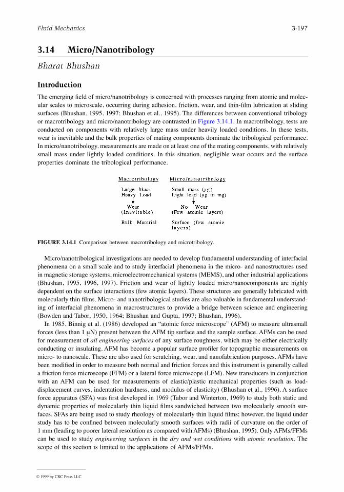
Fluid Mechanics 3-197
3.14 Micro/Nanotribology
Bharat Bhushan
Introduction
The emerging Þeld of micro/nanotribology is concerned with processes ranging from atomic and molec-ular scales to microscale, occurring during adhesion, friction, wear, and thin-Þlm lubrication at slidingsurfaces (Bhushan, 1995, 1997; Bhushan et al., 1995). The differences between conventional tribologyor macrotribology and micro/nanotribology are contrasted in Figure 3.14.1. In macrotribology, tests areconducted on components with relatively large mass under heavily loaded conditions. In these tests,wear is inevitable and the bulk properties of mating components dominate the tribological performance.In micro/nanotribology, measurements are made on at least one of the mating components, with relativelysmall mass under lightly loaded conditions. In this situation, negligible wear occurs and the surfaceproperties dominate the tribological performance.
Micro/nanotribological investigations are needed to develop fundamental understanding of interfacialphenomena on a small scale and to study interfacial phenomena in the micro- and nanostructures usedin magnetic storage systems, microelectromechanical systems (MEMS), and other industrial applications(Bhushan, 1995, 1996, 1997). Friction and wear of lightly loaded micro/nanocomponents are highlydependent on the surface interactions (few atomic layers). These structures are generally lubricated withmolecularly thin Þlms. Micro- and nanotribological studies are also valuable in fundamental understand-ing of interfacial phenomena in macrostructures to provide a bridge between science and engineering(Bowden and Tabor, 1950, 1964; Bhushan and Gupta, 1997; Bhushan, 1996).
In 1985, Binnig et al. (1986) developed an Òatomic force microscopeÓ (AFM) to measure ultrasmallforces (less than 1 mN) present between the AFM tip surface and the sample surface. AFMs can be usedfor measurement of all engineering surfaces of any surface roughness, which may be either electricallyconducting or insulating. AFM has become a popular surface proÞler for topographic measurements onmicro- to nanoscale. These are also used for scratching, wear, and nanofabrication purposes. AFMs havebeen modiÞed in order to measure both normal and friction forces and this instrument is generally calleda friction force microscope (FFM) or a lateral force microscope (LFM). New transducers in conjunctionwith an AFM can be used for measurements of elastic/plastic mechanical properties (such as load-displacement curves, indentation hardness, and modulus of elasticity) (Bhushan et al., 1996). A surfaceforce apparatus (SFA) was Þrst developed in 1969 (Tabor and Winterton, 1969) to study both static anddynamic properties of molecularly thin liquid Þlms sandwiched between two molecularly smooth sur-faces. SFAs are being used to study rheology of molecularly thin liquid Þlms; however, the liquid understudy has to be conÞned between molecularly smooth surfaces with radii of curvature on the order of1 mm (leading to poorer lateral resolution as compared with AFMs) (Bhushan, 1995). Only AFMs/FFMscan be used to study engineering surfaces in the dry and wet conditions with atomic resolution. Thescope of this section is limited to the applications of AFMs/FFMs.
FIGURE 3.14.1 Comparison between macrotribology and microtribology.
© 1999 by CRC Press LLC
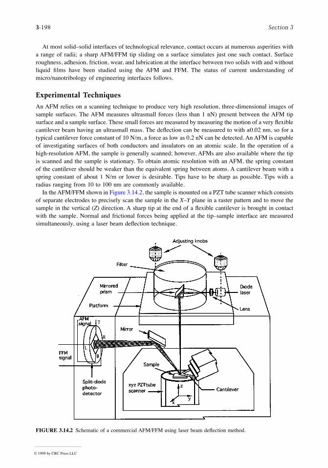
3-198 Section 3
At most solidÐsolid interfaces of technological relevance, contact occurs at numerous asperities witha range of radii; a sharp AFM/FFM tip sliding on a surface simulates just one such contact. Surfaceroughness, adhesion, friction, wear, and lubrication at the interface between two solids with and withoutliquid Þlms have been studied using the AFM and FFM. The status of current understanding ofmicro/nanotribology of engineering interfaces follows.
Experimental Techniques
An AFM relies on a scanning technique to produce very high resolution, three-dimensional images ofsample surfaces. The AFM measures ultrasmall forces (less than 1 nN) present between the AFM tipsurface and a sample surface. These small forces are measured by measuring the motion of a very ßexiblecantilever beam having an ultrasmall mass. The deßection can be measured to with ±0.02 nm, so for atypical cantilever force constant of 10 N/m, a force as low as 0.2 nN can be detected. An AFM is capableof investigating surfaces of both conductors and insulators on an atomic scale. In the operation of ahigh-resolution AFM, the sample is generally scanned; however, AFMs are also available where the tipis scanned and the sample is stationary. To obtain atomic resolution with an AFM, the spring constantof the cantilever should be weaker than the equivalent spring between atoms. A cantilever beam with aspring constant of about 1 N/m or lower is desirable. Tips have to be sharp as possible. Tips with aradius ranging from 10 to 100 nm are commonly available.
In the AFM/FFM shown in Figure 3.14.2, the sample is mounted on a PZT tube scanner which consistsof separate electrodes to precisely scan the sample in the XÐY plane in a raster pattern and to move thesample in the vertical (Z) direction. A sharp tip at the end of a ßexible cantilever is brought in contactwith the sample. Normal and frictional forces being applied at the tipÐsample interface are measuredsimultaneously, using a laser beam deßection technique.
FIGURE 3.14.2 Schematic of a commercial AFM/FFM using laser beam deßection method.
© 1999 by CRC Press LLC
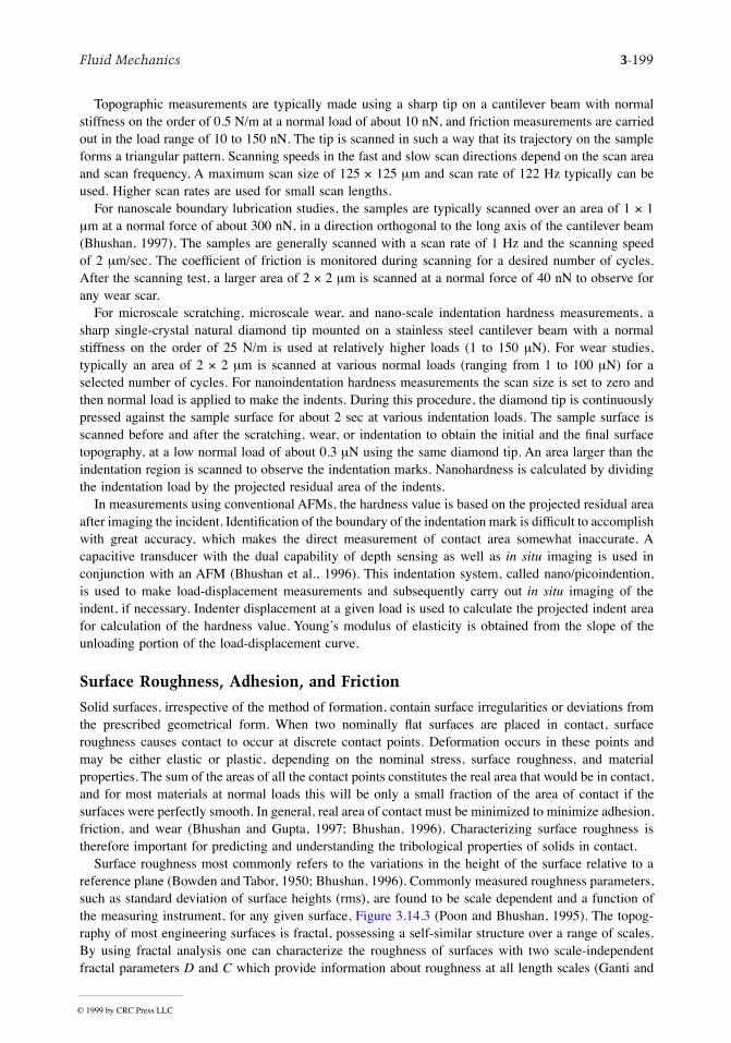
Fluid Mechanics 3-199
Topographic measurements are typically made using a sharp tip on a cantilever beam with normalstiffness on the order of 0.5 N/m at a normal load of about 10 nN, and friction measurements are carriedout in the load range of 10 to 150 nN. The tip is scanned in such a way that its trajectory on the sampleforms a triangular pattern. Scanning speeds in the fast and slow scan directions depend on the scan areaand scan frequency. A maximum scan size of 125 ´ 125 mm and scan rate of 122 Hz typically can beused. Higher scan rates are used for small scan lengths.
For nanoscale boundary lubrication studies, the samples are typically scanned over an area of 1 ´ 1mm at a normal force of about 300 nN, in a direction orthogonal to the long axis of the cantilever beam(Bhushan, 1997). The samples are generally scanned with a scan rate of 1 Hz and the scanning speedof 2 mm/sec. The coefÞcient of friction is monitored during scanning for a desired number of cycles.After the scanning test, a larger area of 2 ´ 2 mm is scanned at a normal force of 40 nN to observe forany wear scar.
For microscale scratching, microscale wear, and nano-scale indentation hardness measurements, asharp single-crystal natural diamond tip mounted on a stainless steel cantilever beam with a normalstiffness on the order of 25 N/m is used at relatively higher loads (1 to 150 mN). For wear studies,typically an area of 2 ´ 2 mm is scanned at various normal loads (ranging from 1 to 100 mN) for aselected number of cycles. For nanoindentation hardness measurements the scan size is set to zero andthen normal load is applied to make the indents. During this procedure, the diamond tip is continuouslypressed against the sample surface for about 2 sec at various indentation loads. The sample surface isscanned before and after the scratching, wear, or indentation to obtain the initial and the Þnal surfacetopography, at a low normal load of about 0.3 mN using the same diamond tip. An area larger than theindentation region is scanned to observe the indentation marks. Nanohardness is calculated by dividingthe indentation load by the projected residual area of the indents.
In measurements using conventional AFMs, the hardness value is based on the projected residual areaafter imaging the incident. IdentiÞcation of the boundary of the indentation mark is difÞcult to accomplishwith great accuracy, which makes the direct measurement of contact area somewhat inaccurate. Acapacitive transducer with the dual capability of depth sensing as well as in situ imaging is used inconjunction with an AFM (Bhushan et al., 1996). This indentation system, called nano/picoindention,is used to make load-displacement measurements and subsequently carry out in situ imaging of theindent, if necessary. Indenter displacement at a given load is used to calculate the projected indent areafor calculation of the hardness value. YoungÕs modulus of elasticity is obtained from the slope of theunloading portion of the load-displacement curve.
Surface Roughness, Adhesion, and Friction
Solid surfaces, irrespective of the method of formation, contain surface irregularities or deviations fromthe prescribed geometrical form. When two nominally ßat surfaces are placed in contact, surfaceroughness causes contact to occur at discrete contact points. Deformation occurs in these points andmay be either elastic or plastic, depending on the nominal stress, surface roughness, and materialproperties. The sum of the areas of all the contact points constitutes the real area that would be in contact,and for most materials at normal loads this will be only a small fraction of the area of contact if thesurfaces were perfectly smooth. In general, real area of contact must be minimized to minimize adhesion,friction, and wear (Bhushan and Gupta, 1997; Bhushan, 1996). Characterizing surface roughness istherefore important for predicting and understanding the tribological properties of solids in contact.
Surface roughness most commonly refers to the variations in the height of the surface relative to areference plane (Bowden and Tabor, 1950; Bhushan, 1996). Commonly measured roughness parameters,such as standard deviation of surface heights (rms), are found to be scale dependent and a function ofthe measuring instrument, for any given surface, Figure 3.14.3 (Poon and Bhushan, 1995). The topog-raphy of most engineering surfaces is fractal, possessing a self-similar structure over a range of scales.By using fractal analysis one can characterize the roughness of surfaces with two scale-independentfractal parameters D and C which provide information about roughness at all length scales (Ganti and
© 1999 by CRC Press LLC
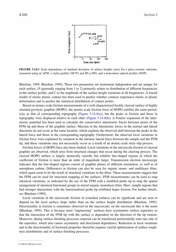
3-200 Section 3
Bhushan, 1995; Bhushan, 1995). These two parameters are instrument independent and are unique foreach surface. D (generally ranging from 1 to 2) primarily relates to distribution of different frequenciesin the surface proÞle, and C to the amplitude of the surface height variations at all frequencies. A fractalmodel of elastic plastic contact has been used to predict whether contacts experience elastic or plasticdeformation and to predict the statistical distribution of contact points.
Based on atomic-scale friction measurements of a well-characterized freshly cleaved surface of highlyoriented pyrolytic graphite (HOPG), the atomic-scale friction force of HOPG exhibits the same period-icity as that of corresponding topography (Figure 3.14.4(a)), but the peaks in friction and those intopography were displaced relative to each other (Figure 3.14.4(b)). A Fourier expansion of the inter-atomic potential has been used to calculate the conservative interatomic forces between atoms of theFFM tip and those of the graphite surface. Maxima in the interatomic forces in the normal and lateraldirections do not occur at the same location, which explains the observed shift between the peaks in thelateral force and those in the corresponding topography. Furthermore, the observed local variations infriction force were explained by variation in the intrinsic lateral force between the sample and the FFMtip, and these variations may not necessarily occur as a result of an atomic-scale stickÐslip process.
Friction forces of HOPG have also been studied. Local variations in the microscale friction of cleavedgraphite are observed, which arise from structural changes that occur during the cleaving process. Thecleaved HOPG surface is largely atomically smooth, but exhibits line-shaped regions in which thecoefÞcient of friction is more than an order of magnitude larger. Transmission electron microscopyindicates that the line-shaped regions consist of graphite planes of different orientation, as well as ofamorphous carbon. Differences in friction can also be seen for organic mono- and multilayer Þlms,which again seem to be the result of structural variations in the Þlms. These measurements suggest thatthe FFM can be used for structural mapping of the surfaces. FFM measurements can be used to mapchemical variations, as indicated by the use of the FFM with a modiÞed probe tip to map the spatialarrangement of chemical functional groups in mixed organic monolayer Þlms. Here, sample regions thathad stronger interactions with the functionalized probe tip exhibited larger friction. For further details,see Bhushan (1995).
Local variations in the microscale friction of scratched surfaces can be signiÞcant and are seen todepend on the local surface slope rather than on the surface height distribution (Bhushan, 1995).Directionality in friction is sometimes observed on the macroscale; on the microscale this is the norm(Bhushan, 1995). This is because most ÒengineeringÓ surfaces have asymmetric surface asperities sothat the interaction of the FFM tip with the surface is dependent on the direction of the tip motion.Moreover, during surface-Þnishing processes material can be transferred preferentially onto one side ofthe asperities, which also causes asymmetry and directional dependence. Reduction in local variationsand in the directionality of frictional properties therefore requires careful optimization of surface rough-ness distributions and of surface-Þnishing processes.
FIGURE 3.14.3 Scale dependence of standard deviation of surface heights (rms) for a glassÐceramic substrate,measured using an AFM, a stylus proÞler (SP-P2 and SP-a 200), and a noncontact optical proÞler (NOP).
© 1999 by CRC Press LLC
Fluid Mechanics 3-201
Table 3.14.1 shows the coefÞcient of friction measured for two surfaces on micro- and macroscales.The coefÞcient of friction is deÞned as the ratio of friction force to the normal load. The values on themicroscale are much lower than those on the macroscale. When measured for the small contact areasand very low loads used in microscale studies, indentation hardness and modulus of elasticity are higherthan at the macroscale. This reduces the degree of wear. In addition, the small apparent areas of contactreduce the number of particles trapped at the interface, and thus minimize the ÒploughingÓ contributionto the friction force.
At higher loads (with contact stresses exceeding the hardness of the softer material), however, thecoefÞcient of friction for microscale measurements increases toward values comparable with thoseobtained from macroscale measurements, and surface damage also increases (Bhushan et al., 1995;Bhushan and Kulkarni, 1996). Thus, AmontonsÕ law of friction, which states that the coefÞcient of
a
b
FIGURE 3.14.4 (a) Gray-scale plots of surface topography (left) and friction proÞles (right) of a 1 ´ 1 nm area offreshly cleaved HOPG, showing the atomic-scale variation of topography and friction, (b) diagram of superimposedtopography and friction proÞles from (a); the symbols correspond to maxima. Note the spatial shift between the twoproÞles.
Sliding direction
1 nm
1 nm
Topography Friction
© 1999 by CRC Press LLC
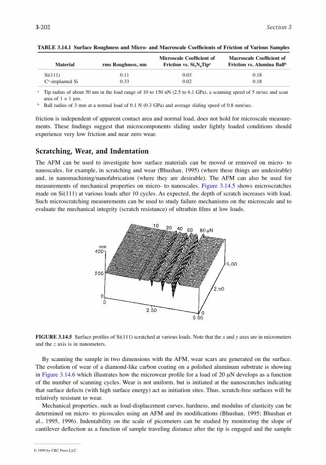
3-202 Section 3
friction is independent of apparent contact area and normal load, does not hold for microscale measure-ments. These Þndings suggest that microcomponents sliding under lightly loaded conditions shouldexperience very low friction and near zero wear.
Scratching, Wear, and Indentation
The AFM can be used to investigate how surface materials can be moved or removed on micro- tonanoscales, for example, in scratching and wear (Bhushan, 1995) (where these things are undesirable)and, in nanomachining/nanofabrication (where they are desirable). The AFM can also be used formeasurements of mechanical properties on micro- to nanoscales. Figure 3.14.5 shows microscratchesmade on Si(111) at various loads after 10 cycles. As expected, the depth of scratch increases with load.Such microscratching measurements can be used to study failure mechanisms on the microscale and toevaluate the mechanical integrity (scratch resistance) of ultrathin Þlms at low loads.
By scanning the sample in two dimensions with the AFM, wear scars are generated on the surface.The evolution of wear of a diamond-like carbon coating on a polished aluminum substrate is showingin Figure 3.14.6 which illustrates how the microwear proÞle for a load of 20 mN develops as a functionof the number of scanning cycles. Wear is not uniform, but is initiated at the nanoscratches indicatingthat surface defects (with high surface energy) act as initiation sites. Thus, scratch-free surfaces will berelatively resistant to wear.
Mechanical properties, such as load-displacement curves, hardness, and modulus of elasticity can bedetermined on micro- to picoscales using an AFM and its modiÞcations (Bhushan, 1995; Bhushan etal., 1995, 1996). Indentability on the scale of picometers can be studied by monitoring the slope ofcantilever deßection as a function of sample traveling distance after the tip is engaged and the sample
TABLE 3.14.1 Surface Roughness and Micro- and Macroscale CoefÞcients of Friction of Various Samples
Material rms Roughness, nmMicroscale CoefÞcient of
Friction vs. Si3N4Tipa
Macroscale CoefÞcient of Friction vs. Alumina Ballb
Si(111) 0.11 0.03 0.18C+-implanted Si 0.33 0.02 0.18
a Tip radius of about 50 nm in the load range of 10 to 150 nN (2.5 to 6.1 GPa), a scanning speed of 5 m/sec and scan area of 1 ´ 1 mm.
b Ball radius of 3 mm at a normal load of 0.1 N (0.3 GPa) and average sliding speed of 0.8 mm/sec.
FIGURE 3.14.5 Surface proÞles of Si(111) scratched at various loads. Note that the x and y axes are in micrometersand the z axis is in nanometers.
© 1999 by CRC Press LLC
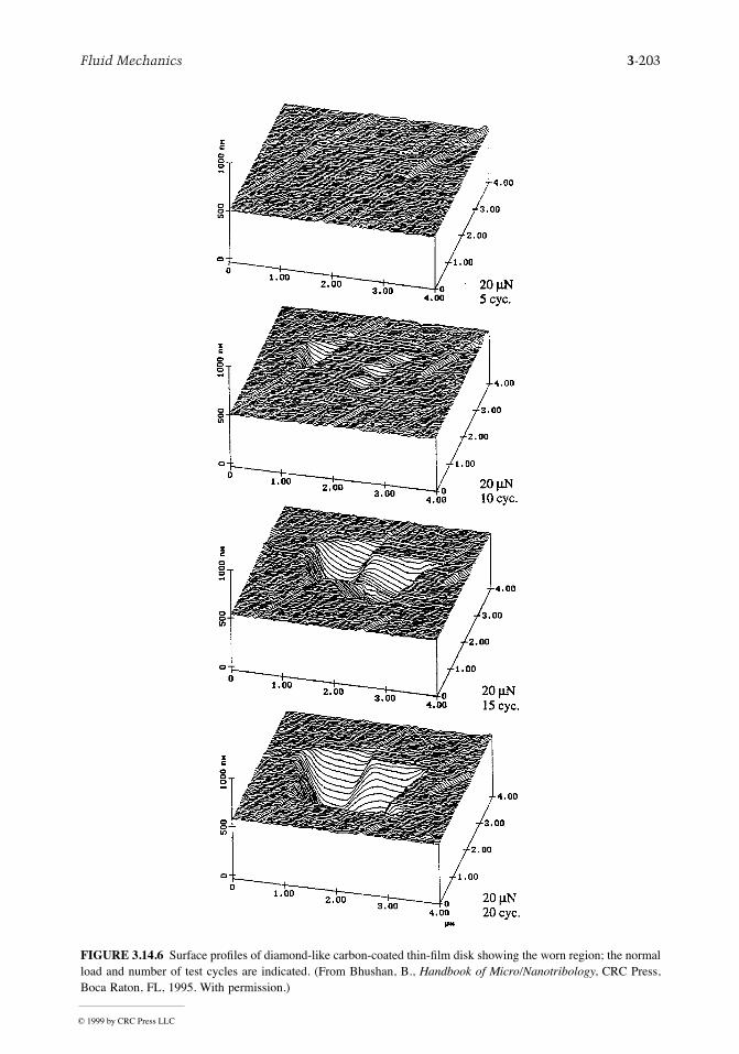
Fluid Mechanics 3-203
FIGURE 3.14.6 Surface proÞles of diamond-like carbon-coated thin-Þlm disk showing the worn region; the normalload and number of test cycles are indicated. (From Bhushan, B., Handbook of Micro/Nanotribology, CRC Press,Boca Raton, FL, 1995. With permission.)
© 1999 by CRC Press LLC
3-204 Section 3
is pushed against the tip. For a rigid sample, cantilever deßection equals the sample traveling distance;but the former quantity is smaller if the tip indents the sample. The indentation hardness on nanoscaleof bulk materials and surface Þlms with an indentation depth as small as 1 nm can be measured. Anexample of hardness data as a function of indentation depth is shown in Figure 3.14.7. A decrease inhardness with an increase in indentation depth can be rationalized on the basis that, as the volume ofdeformed materials increases, there is a higher probability of encountering material defects. AFMmeasurements on ion-implanted silicon surfaces show that ion implantation increases their hardness and,thus, their wear resistance (Bhushan, 1995). Formation of surface alloy Þlms with improved mechanicalproperties by ion implantation is growing in technological importance as a means of improving themechanical properties of materials.
YoungÕs modulus of elasticity is calculated from the slope of the indentation curve during unloading(Bhushan, 1995; Bhushan et al., 1996). AFM can be used in a force modulation mode to measure surfaceelasticities: an AFM tip is scanned over the modulated sample surface with the feedback loop keepingthe average force constant. For the same applied force, a soft area deforms more, and thus causes lesscantilever deßection, than a hard area. The ratio of modulation amplitude to the local tip deßection isthen used to create a force modulation image. The force modulation mode makes it easier to identifysoft areas on hard substrates.
Detection of the transfer of material on a nanoscale is possible with the AFM. Indentation of C60-richfullerene Þlms with an AFM tip has been shown to result in the transfer of fullerene molecules to theAFM tip, as indicated by discontinuities in the cantilever deßection as a function of sample travelingdistance in subsequent indentation studies (Bhushan, 1995).
Boundary Lubrication
The ÒclassicalÓ approach to lubrication uses freely supported multimolecular layers of liquid lubricants(Bowden and Tabor, 1950, 1964; Bhushan, 1996). The liquid lubricants are chemically bonded to improvetheir wear resistance (Bhushan, 1995, 1996). To study depletion of boundary layers, the microscalefriction measurements are made as a function of the number of cycles. For an example of the data ofvirgin Si(100) surface and silicon surface lubricated with about 2-nm-thick Z-15 and Z-Dol perßuo-ropolyether (PEPE) lubricants, see Figure 3.14.8. Z-Dol is PFPE lubricant with hydroxyl end groups.Its lubricant Þlm was thermally bonded. In Figure 3.14.8, the unlubricated silicon sample shows a slightincrease in friction force followed by a drop to a lower steady state value after some cycles. Depletionof native oxide and possible roughening of the silicon sample are responsible for the decrease in this
FIGURE 3.14.7 Indentation hardness as a function of residual indentation depth for Si(100).
© 1999 by CRC Press LLC
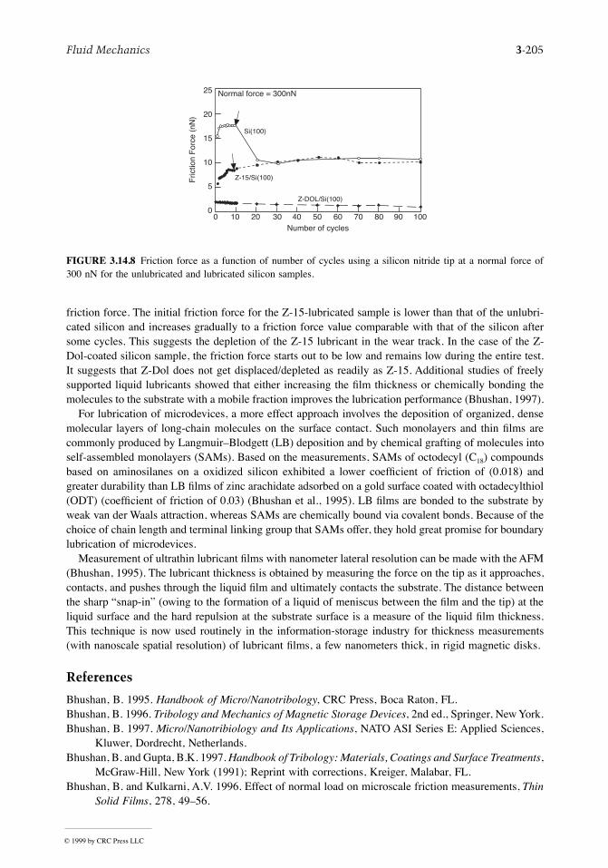
Fluid Mechanics 3-205
friction force. The initial friction force for the Z-15-lubricated sample is lower than that of the unlubri-cated silicon and increases gradually to a friction force value comparable with that of the silicon aftersome cycles. This suggests the depletion of the Z-15 lubricant in the wear track. In the case of the Z-Dol-coated silicon sample, the friction force starts out to be low and remains low during the entire test.It suggests that Z-Dol does not get displaced/depleted as readily as Z-15. Additional studies of freelysupported liquid lubricants showed that either increasing the Þlm thickness or chemically bonding themolecules to the substrate with a mobile fraction improves the lubrication performance (Bhushan, 1997).
For lubrication of microdevices, a more effect approach involves the deposition of organized, densemolecular layers of long-chain molecules on the surface contact. Such monolayers and thin Þlms arecommonly produced by LangmuirÐBlodgett (LB) deposition and by chemical grafting of molecules intoself-assembled monolayers (SAMs). Based on the measurements, SAMs of octodecyl (C18) compoundsbased on aminosilanes on a oxidized silicon exhibited a lower coefÞcient of friction of (0.018) andgreater durability than LB Þlms of zinc arachidate adsorbed on a gold surface coated with octadecylthiol(ODT) (coefÞcient of friction of 0.03) (Bhushan et al., 1995). LB Þlms are bonded to the substrate byweak van der Waals attraction, whereas SAMs are chemically bound via covalent bonds. Because of thechoice of chain length and terminal linking group that SAMs offer, they hold great promise for boundarylubrication of microdevices.
Measurement of ultrathin lubricant Þlms with nanometer lateral resolution can be made with the AFM(Bhushan, 1995). The lubricant thickness is obtained by measuring the force on the tip as it approaches,contacts, and pushes through the liquid Þlm and ultimately contacts the substrate. The distance betweenthe sharp Òsnap-inÓ (owing to the formation of a liquid of meniscus between the Þlm and the tip) at theliquid surface and the hard repulsion at the substrate surface is a measure of the liquid Þlm thickness.This technique is now used routinely in the information-storage industry for thickness measurements(with nanoscale spatial resolution) of lubricant Þlms, a few nanometers thick, in rigid magnetic disks.
References
Bhushan, B. 1995. Handbook of Micro/Nanotribology, CRC Press, Boca Raton, FL.Bhushan, B. 1996. Tribology and Mechanics of Magnetic Storage Devices, 2nd ed., Springer, New York.Bhushan, B. 1997. Micro/Nanotribiology and Its Applications, NATO ASI Series E: Applied Sciences,
Kluwer, Dordrecht, Netherlands.Bhushan, B. and Gupta, B.K. 1997. Handbook of Tribology: Materials, Coatings and Surface Treatments,
McGraw-Hill, New York (1991); Reprint with corrections, Kreiger, Malabar, FL.Bhushan, B. and Kulkarni, A.V. 1996. Effect of normal load on microscale friction measurements, Thin
Solid Films, 278, 49Ð56.
FIGURE 3.14.8 Friction force as a function of number of cycles using a silicon nitride tip at a normal force of300 nN for the unlubricated and lubricated silicon samples.
25
20
15
10
5
0
Fric
tion
For
ce (
nN)
Normal force = 300nN
0 10 20 30 40 50 60 70 80 90 100Number of cycles
Z-DOL/Si(100)
Z-15/Si(100)
Si(100)
© 1999 by CRC Press LLC
3-206 Section 3
Bhushan, B., Israelachvili, J.N., and Landman, U. 1995. Nanotribology: friction, wear and lubricationat the atomic scale, Nature, 374, 607Ð616.
Bhushan, B., Kulkarni, A.V., Bonin, W., and Wyrobek, J.T. 1996. Nano-indentation and pico-indentationmeasurements using capacitive transducer system in atomic force microscopy, Philos. Mag., A74,1117Ð1128.
Binning, G., Quate, C.F., and Gerber, Ch. 1986. Atomic force microscopy, Phys. Rev. Lett., 56, 930Ð933.Bowden, F.P. and Tabor, D. 1950; 1964. The Friction and Lubrication of Solids, Parts I and II, Clarendon,
Oxford.Ganti, S. and Bhushan, B. 1995. Generalized fractal analysis and its applications to engineering surfaces,
Wear, 180, 17Ð34.Poon, C.Y. and Bhushan, B. 1995. Comparison of surface roughness measurements by stylus proÞler,
AFM and non-contact optical proÞler, Wear, 190, 76Ð88.Tabor, D. and Winterton, R.H.S. 1969. The direct measurement of normal and retarded van der Walls
forces, Proc. R. Soc. London, A312, 435Ð450.
Nomenclature for Fluid Mechanics
Unit
Symbol Quantity SI English Dimensions (MLtT)
a Velocity of sound m/sec ft/sec LtÐ1
a Acceleration m/sec2 ft/sec2 LtÐ2
A Area m2 ft2 L2
b Distance, width m ft Lcp SpeciÞc heat, constant pressure J/kgáK ftálb/lbmá°R L2tÐ2TÐ1
cv SpeciÞc heat, constant volume J/kgáK ftálb/lbmá°R L2tÐ2TÐ1
C Concentration No./m3 No./ft3 LÐ3
C CoefÞcient Ñ Ñ ÑC Empirical constant Ñ Ñ ÑD Diameter m ft LDH Hydraulic diameter m ft Le Total energy per unit mass J/kg ftálb/lbm L2tÐ2
E Total energy J ftálb or Btu ML2tÐ2
E Modulus of leasticity Pa lb/ft2 ML1tÐ2
Eu Euler number Ñ Ñ Ñf Friction factor Ñ Ñ ÑF Force N lb MLtÐ2
Fr Froude number Ñ Ñ ÑFB Buoyant force N lb MLtÐ2
g Acceleration of gravity m/sec2 ft/sec2 LtÐ2
g0 Gravitation constant kgám/Násec2 lbmáft/lbásec2 ÑG Mass ßow rate per unit area kg/secám2 lbm/secáft2 MLÐ2tÐ1
h Head, vertical distance m ft Lh Enthalpy per unit mass J/kg ftálb/lbm L2tÐ2
H Head, elevation of hydraulic grade line m ft LI Moment of inertia m4 ft4 L4
k SpeciÞc heat ratio Ñ Ñ ÑK Bulk modulus of elasticity Pa lb/ft2 ML1tÐ2
K Minor loss coefÞcient Ñ Ñ ÑL Length m ft LL Lift N lb MLtÐ2
l Length, mixing length m ft Lln Natural logarithm Ñ Ñ Ñm Mass kg lbm M
Strength of source m3/sec ft3/sec L3tÐ1
m Mass ßow rate kg/sec lbm/sec MtÐ1
Çm
© 1999 by CRC Press LLC
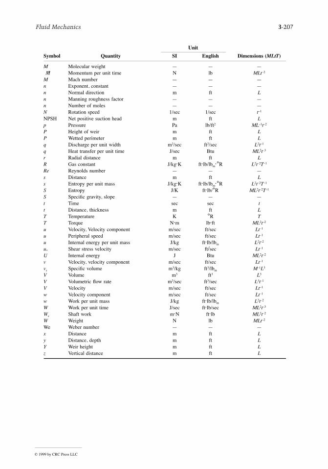
Fluid Mechanics 3-207
M Molecular weight Ñ Ñ ÑMomentum per unit time N lb MLtÐ2
M Mach number Ñ Ñ Ñn Exponent, constant Ñ Ñ Ñn Normal direction m ft Ln Manning roughness factor Ñ Ñ Ñn Number of moles Ñ Ñ ÑN Rotation speed 1/sec 1/sec tÐ1
NPSH Net positive suction head m ft Lp Pressure Pa lb/ft2 MLÐ1tÐ2
P Height of weir m ft LP Wetted perimeter m ft Lq Discharge per unit width m2/sec ft2/sec L2tÐ1
q Heat transfer per unit time J/sec Btu ML2tÐ3
r Radial distance m ft LR Gas constant J/kgáK ftálb/lbmá°R L2tÐ2TÐ1
Re Reynolds number Ñ Ñ Ñs Distance m ft Ls Entropy per unit mass J/kgáK ftálb/lbmá°R L2tÐ2TÐ1
S Entropy J/K ftálb/°R ML2tÐ2TÐ1
S SpeciÞc gravity, slope Ñ Ñ Ñt Time sec sec tt Distance, thickness m ft LT Temperature K °R TT Torque Nám lbáft ML2tÐ2
u Velocity, Velocity component m/sec ft/sec LtÐ1
u Peripheral speed m/sec ft/sec LtÐ1
u Internal energy per unit mass J/kg ftálb/lbm L2tÐ2
u* Shear stress velocity m/sec ft/sec LtÐ1
U Internal energy J Btu ML2tÐ2
v Velocity, velocity component m/sec ft/sec LtÐ1
vs SpeciÞc volume m3/kg ft3/lbm MÐ1L3
V Volume m3 ft3 L3
V Volumetric ßow rate m3/sec ft3/sec L3tÐ1
V Velocity m/sec ft/sec LtÐ1
w Velocity component m/sec ft/sec LtÐ1
w Work per unit mass J/kg ftálb/lbm L2tÐ2
W Work per unit time J/sec ftálb/sec ML2tÐ3
Ws Shaft work máN ftálb ML2tÐ2
W Weight N lb MLtÐ2
We Weber number Ñ Ñ Ñx Distance m ft Ly Distance, depth m ft LY Weir height m ft Lz Vertical distance m ft L
Unit
Symbol Quantity SI English Dimensions (MLtT)
ÇM
© 1999 by CRC Press LLC
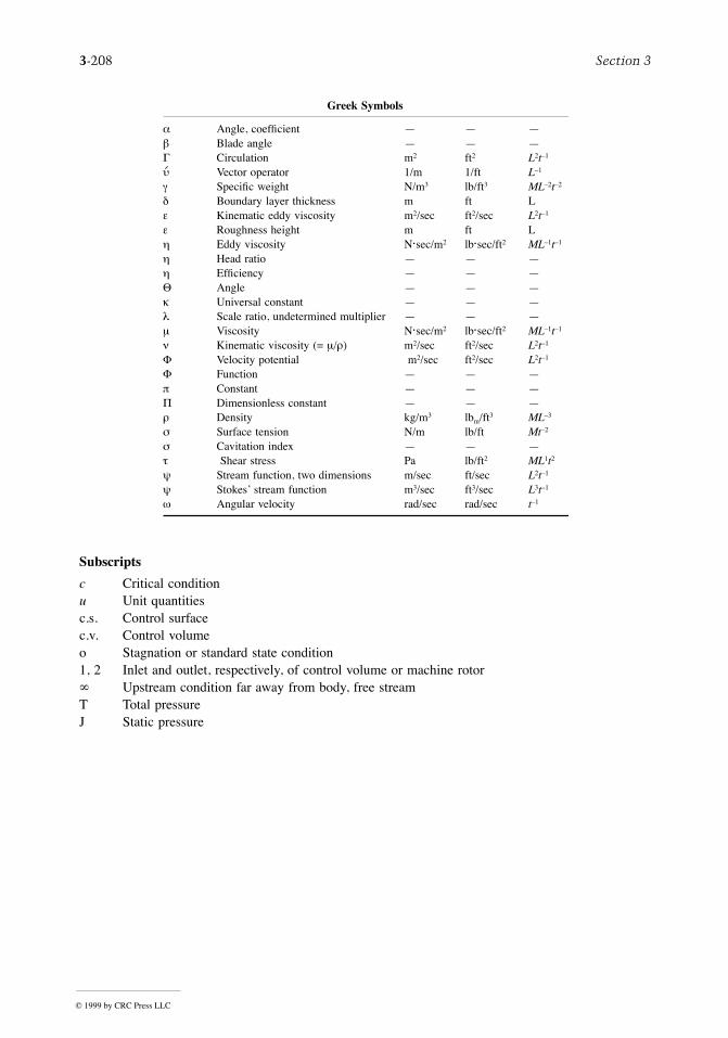
3-208 Section 3
Subscripts
c Critical conditionu Unit quantitiesc.s. Control surfacec.v. Control volumeo Stagnation or standard state condition1, 2 Inlet and outlet, respectively, of control volume or machine rotor¥ Upstream condition far away from body, free streamT Total pressureJ Static pressure
Greek Symbols
a Angle, coefÞcient Ñ Ñ Ñb Blade angle Ñ Ñ ÑG Circulation m2 ft2 L2tÐ1
u Vector operator 1/m 1/ft LÐ1
g SpeciÞc weight N/m3 lb/ft3 MLÐ2tÐ2
d Boundary layer thickness m ft Le Kinematic eddy viscosity m2/sec ft2/sec L2tÐ1
e Roughness height m ft Lh Eddy viscosity Násec/m2 lbásec/ft2 MLÐ1tÐ1
h Head ratio Ñ Ñ Ñh EfÞciency Ñ Ñ ÑQ Angle Ñ Ñ Ñk Universal constant Ñ Ñ Ñl Scale ratio, undetermined multiplier Ñ Ñ Ñm Viscosity Násec/m2 lbásec/ft2 MLÐ1tÐ1
n Kinematic viscosity (= m/r) m2/sec ft2/sec L2tÐ1
F Velocity potential m2/sec ft2/sec L2tÐ1
F Function Ñ Ñ Ñp Constant Ñ Ñ ÑP Dimensionless constant Ñ Ñ Ñr Density kg/m3 lbm/ft3 MLÐ3
s Surface tension N/m lb/ft MtÐ2
s Cavitation index Ñ Ñ Ñt Shear stress Pa lb/ft2 ML1t2
y Stream function, two dimensions m/sec ft/sec L2tÐ1
y StokesÕ stream function m3/sec ft3/sec L3tÐ1
w Angular velocity rad/sec rad/sec tÐ1
© 1999 by CRC Press LLC