KRAVITZ ET AL.: ARCTIC SPRING GEOENGINEERINGclimate.envsci.rutgers.edu/pdf/ArcticSpring.pdf ·...

KRAVITZ ET AL.: ARCTIC SPRING GEOENGINEERING

- 1 -

Climate Model Simulations of Stratospheric Geoengineering in the Arctic Spring 1 2 3

Ben Kravitz, Alan Robock, and Allison Marquardt 4 5 6

Department of Environmental Sciences, Rutgers University, New Brunswick, New Jersey 7 8 9 10 11 12 13 14 15 16 17 18

Submitted to Journal of Geophysical Research - Atmospheres 19 20

September, 2010 21 22 23 24 25 26 27 28 29 30 Ben Kravitz, Department of Environmental Sciences, Rutgers University, 14 College Farm 31

Road, New Brunswick, NJ 08901, USA. ([email protected]) (Corresponding 32 Author) 33

34 Alan Robock, Department of Environmental Sciences, Rutgers University, 14 College Farm 35

Road, New Brunswick, NJ 08901, USA. ([email protected]) 36 37 Allison Marquardt, Department of Environmental Sciences, Rutgers University, 14 College Farm 38

Road, New Brunswick, NJ 08901, USA. ([email protected]) 39 40 41

42


- 2 -

Abstract 43 We use a general circulation model of Earth’s climate to conduct simulations of 44

stratospheric sulfate aerosol geoengineering in the Arctic spring to determine whether 45

geoengineering during the months of maximum insolation is as effective as geoengineering year-46

round. As control cases, we simulate a global warming ensemble and an ensemble of global 47

warming combined with daily stratospheric injections of SO2 at high latitude, totaling 3 Tg SO2 48

per year. We compare these to two ensembles, each with global warming forcing and high 49

latitude stratospheric injections of 0.75 Tg SO2 per year: daily injections throughout April, May, 50

and June; and daily injections throughout April. These spring injection experiments show 51

smaller aerosol optical depth than the year-round injections, especially in the winter, during 52

which all of the sulfate aerosols from the spring injection experiments are removed each year. 53

They also show summer cooling over the Northern Hemisphere continents, as is seen in large 54

volcanic eruptions, although not as much as in the year-round injections. No significant 55

monsoonal precipitation perturbation is detected, in contrast to previous simulations with this 56

same model. Year-round injection results in an increase in Arctic sea ice from a control 57

scenario, and the spring injection experiments show reduced sea ice loss from the global 58

warming simulations. Further simulations are required, but these results suggest that while SO2 59

injections only in the spring are not as effective as year-round injections, a strategy of injections 60

in spring and summer combined would maximize the cooling of the aerosol cloud, requiring 61

slightly smaller total annual injections than a year-round strategy. 62

63


- 3 -

1. Introduction 64

Geoengineering with stratospheric sulfate aerosols has been proposed [e.g., Crutzen, 65

2006] as a cheap [e.g., Robock et al., 2009], effective [e.g., Rasch et al., 2008], and temporary 66

[e.g., Wigley, 2006] means of reducing global average surface air temperature to alleviate 67

negative climate impacts from increasing greenhouse gas concentrations. In an effort to tailor 68

geoengineering and reduce the degree to which humans directly interfere with and modify the 69

climate, some have suggested geoengineering only in the Arctic [Caldeira and Wood, 2008]. 70

They propose that this would have the effect of cooling the Northern Hemisphere continents and 71

potentially “saving” the Arctic sea ice, as is seen temporarily in the case of large volcanic 72

eruptions, but would not impact temperatures in the tropics or the Southern Hemisphere. Due to 73

the reduced area needing to be shaded by sulfate aerosols, geoengineering in the Arctic would in 74

theory require smaller injections of SO2 than geoengineering in the tropics. 75

Robock et al. [2008] performed simulations of both tropical and Arctic geoengineering. 76

They found features similar to those of large volcanic eruptions: summer cooling over the 77

Northern Hemisphere continents and weakening of the Indian/African summer monsoon, which 78

was more pronounced for the case of the Arctic injection. 79

These simulations by Robock et al. involved year-round injections of SO2. However, in 80

the Arctic, year-round injections would not be necessary, as there is no sunlight for the aerosols 81

to backscatter during the winter. This motivated our study to investigate Arctic geoengineering 82

that is tailored to backscatter solar radiation only during the summer, which is the period of 83

maximum insolation. 84

In addition to replicating the Arctic injection experiment from Robock et al. [2008], we 85

designed two additional experiments of geoengineering only in the Arctic spring. Assuming the 86


- 4 -

same daily rate of injection as the year-round experiment, this would reduce the amount of SO2 87

that is injected into the stratosphere, lowering the cost and the degree to which humans directly 88

interfere with the climate system. However, we hypothesize that since the aerosols would be 89

present during summer, the radiative effects of the aerosols would be similar to those of a year-90

round injection. We also wished to investigate whether the Asian/African monsoon system is 91

negatively impacted under these scenarios and whether they can prevent the loss of Arctic sea 92

ice. 93

2. Experiment 94

We conducted simulations with the coupled atmosphere-ocean general circulation model 95

ModelE, which was developed by the National Aeronautics and Space Administration Goddard 96

Institute for Space Studies [Schmidt et al., 2006]. We used the stratospheric version with 4° 97

latitude by 5° longitude horizontal resolution and 23 vertical levels up to 80 km. It is fully 98

coupled to a 4° latitude by 5° longitude dynamic ocean with 13 vertical levels [Russell et al., 99

1995]. 100

The aerosol module [Koch et al., 2006] accounts for SO2 conversion to sulfate aerosols, 101

as well as transport and removal of the aerosols. The chemical model calculates the sulfur cycle 102

in the stratosphere, where the conversion rate of SO2 to sulfate is based on the respective 103

concentrations of SO2 and the hydroxyl radical, the latter of which is prescribed [Oman et al., 104

2006a]. We specified the dry aerosol effective radius to be 0.25 µm, which is the value used for 105

simulation of past volcanic eruptions and geoengineering. The model hydrates the aerosols 106

based on ambient humidity values according to formulas prescribed by Tang [1996], resulting in 107

a distribution of hydrated aerosols with an effective radius of approximately 0.30-0.35 µm, 108

which is consistent with the findings of Stothers [1997]. Radiative forcing from the aerosols is 109


- 5 -

fully interactive with the atmospheric circulation and in our paper is the conventional one as 110

defined by the Intergovernmental Panel on Climate Change [IPCC, 2001], also called “adjusted 111

forcing” (Fa) by Hansen et al. [2005]. For more details, we refer the reader to Kravitz et al. 112

[2010a], which used the same model version and setup. 113

This version of ModelE has been successfully used in the past to simulate both volcanic 114

eruptions and geoengineering. Simulations have been conducted for the eruptions of Laki in 115

1783-1784 [Oman et al., 2006a, 2006b], Katmai in 1912 [Oman et al., 2005], Pinatubo in 1991 116

[Robock et al., 2007], and the recent eruption of Kasatochi in 2008 [Kravitz et al., 2010a]. In all 117

of these cases, ModelE was shown to be reliable in recreating the climate impacts of the 118

eruption. Moreover, Robock et al. [2008] used this model to simulate geoengineering, and 119

results from this study agreed with similar experiments performed by the Hadley Centre [Jones 120

et al., 2010]. Therefore, we are confident in this model’s ability to simulate geoengineering to a 121

degree of accuracy that is scientifically useful. 122

We used the same version of ModelE that was used by Robock et al. [2008], using the 123

same specifications except for two tuning parameters and the atmospheric and oceanic initial 124

conditions. Robock et al. used atmospheric and oceanic conditions from the year 1999, whereas 125

we used those conditions from the year 2007. The current version of ModelE was tuned by 126

modifying two parameters that change planetary albedo, and hence, the net radiation of the 127

planet. This model was tuned because Robock et al. detected a significant temperature trend 128

during the period over which they conducted their simulations, due to insufficient time allowed 129

for model spin-up. These tuning parameters modify the critical humidities for ice cloud and 130

water cloud condensation. Specifically, Robock et al. used tuning parameters U00ice=0.590 and 131

U00wtrx=1.33. The version used for the simulations in our study used parameters U00ice=0.595 132


- 6 -

and U00wtrx=1.40. Before simulations were performed with these new parameters, the model 133

was spun-up for an additional 100 years. This resulted in a much smaller trend over the model 134

period 2007-2026, and, after conducting further simulation with a control run, the temperature 135

trend under these new tuning parameters is largely negligible. In Section 5, we discuss the 136

effects this tuning had on our results. 137

We began with a 6-member control ensemble of 20-year runs (2007-2026), during which 138

global greenhouse gas concentrations, as well as aerosol concentrations, remained fixed at 139

constant 2007 conditions. We then simulated a 6-member ensemble of 20-year runs covering the 140

same period, in which global greenhouse gas concentrations increased according to the IPCC’s 141

A1B scenario [IPCC, 2007]. The greenhouse gas concentrations at the beginning of the 142

simulation were prescribed to be January 1, 2007 levels, and they increased to the A1B 143

scenario’s estimation of December 31, 2026 levels by the end of the simulation. 144

We conducted three 6-member ensembles of 20-year runs to simulate geoengineering, all 145

of which had the A1B greenhouse gas concentrations as a background. One ensemble involved 146

daily injections of 0.0082 Tg of SO2 into one grid box centered at 66°N, 122.5°E in the Arctic, 147

distributed equally in the three model layers that cover an altitude of 10-16 km. This 148

corresponds to an annual injection rate of 3 Tg of SO2, so we refer to this ensemble in the rest of 149

the paper as 3 Tg. This ensemble is conducted in the same manner as the Arctic geoengineering 150

scenario described by Robock et al. [2008], albeit with different initial conditions and tuning 151

parameters, which we describe below. Another ensemble, referred to as AMJ, involved daily 152

injections of the same amount at the same spatial points, but only in the months April, May, and 153

June. This results in a total injection rate of 0.75 Tg of SO2 per year. The third ensemble, 154

referred to as Apr, also results in a total injection rate of 0.75 Tg of SO2 per year, but the daily 155


- 7 -

injections occurred only in the month of April. This corresponds to a daily rate of injection of 156

0.0246 Tg, or three times the rate of the previous ensembles. The specifications for the different 157

ensembles are summarized in Table 1. 158

3. Climate Forcing 159

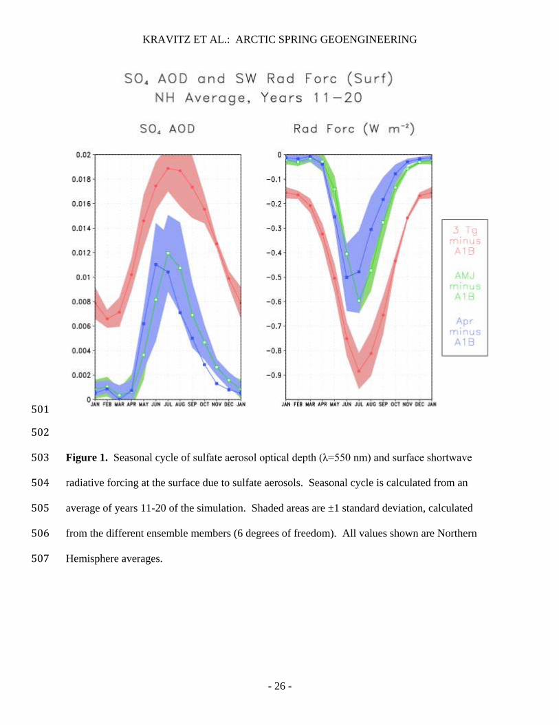
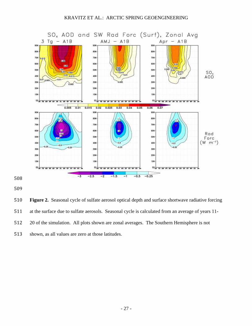
Figures 1 and 2 show the seasonal cycle, averaged over the second decade of simulation, 160

of sulfate aerosol optical depth and radiative forcing once the aerosol layer has achieved a steady 161

state. As with high latitude volcanic eruptions [Kravitz and Robock, 2010] and prior simulation 162

of Arctic geoengineering [Robock et al., 2008], the bulk of the aerosol cloud is mostly confined 163

to latitudes north of 30°N. 164

There is a large seasonal dependence of aerosol optical depth and, consequently, aerosol 165

radiative forcing. All geoengineering simulations show a strong summer peak in optical depth 166

during the summer, which is due to the chemical conversion time of SO2 to sulfate of 30-40 days 167

[McKeen et al., 1984]. In contrast to 3 Tg, AMJ and Apr show all sulfate aerosols are deposited 168

out of the atmosphere throughout the winter and are replenished each spring. In 3 Tg, aerosols 169

are created year-round in the mid-latitudes and throughout the summer, autumn, and early spring 170

in the high latitudes, resulting in a higher peak of aerosol optical depth and even some 171

maintenance of aerosol optical depth in the winter. AMJ and Apr do not have these sources of 172

year-round replenishment, so the aerosols are subjected to unmitigated large-scale removal, and 173

the magnitude of injection is insufficient to allow the aerosols to persist into the following spring 174

[Kravitz and Robock, 2010]. 175

Even though the amount of SO2 injected is the same in both AMJ and Apr, the AMJ 176

ensemble reaches higher peaks of aerosol optical depth and radiative forcing. The AMJ peak 177

occurs in July, which is consistent with the one-month chemical lifetime of stratospheric SO2. 178


- 8 -

This means that the daily injection rate and subsequent SO4 formation rate in the AMJ 179

experiment is greater than the late spring/early summer aerosol deposition rate at high latitudes. 180

The optical depths at mid-latitudes are nearly identical between the two spring injection 181

experiments, suggesting the difference between these two scenarios mostly occurs at high 182

latitudes. The optical depth from Apr is higher throughout the spring than AMJ, since the total 183

amount of SO2 injected under Apr is larger than AMJ until the end of June. 184

4. Climate Response 185

With both simulations of volcanic eruptions [Kravitz and Robock, 2010] and 186

geoengineering [e.g., Robock et al., 2008], an introduction of sulfate aerosols into the 187

stratosphere would cause an observable climate response if the injection is large enough, at the 188

proper time of year [Kravitz and Robock, 2010], or if the injection is continued for a long enough 189

period of time [Robock et al., 2010]. The main purpose of geoengineering would be to cool the 190

planet, so one of the primary climate responses should be a reduction in surface air temperature, 191

as is seen from large volcanic eruptions. This modifies dynamics in the Asian/African monsoon 192

region by reducing the land-ocean temperature gradient. Since this gradient is the primary driver 193

of monsoonal precipitation, geoengineering should weaken the monsoon. We discuss this 194

mechanism of precipitation reduction in more detail in the following section. 195

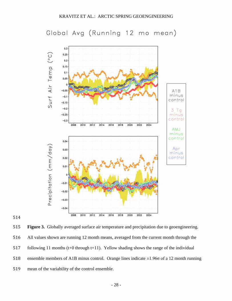
Figure 3 shows globally averaged temperature and precipitation over the simulated period 196

for all experiments. All three geoengineering scenarios show some cooling below A1B 197

temperatures, the strongest and most discernible cooling being from 3 Tg. The results from this 198

experiment are very similar to those in Robock et al. [2008]. Conversely, and contrarily to the 199

findings of Robock et al., none of the simulations, including the 3 Tg experiment, show a 200

reduction in globally averaged precipitation from a global warming situation, although all of the 201


- 9 -

ensembles do show statistically significant anomalies when compared to the control ensemble. 202

Trenberth and Dai [2007] argue that geoengineering would indeed cause a reduction in 203

precipitation, as is seen in the case of large volcanic eruptions, which is in concordance with the 204

results of Robock et al. 205

The classical climate responses to large high latitude volcanic eruptions have spatial 206

patterns as well as global average anomalies. Specifically, these patterns are summer cooling 207

over the Northern Hemisphere continents and a weakening of the Indian/African monsoon 208

system, both of which were found by Robock et al. [2008] in their simulations of Arctic 209

geoengineering. Similarly, in our 3 Tg experiment, we found summer cooling over the Northern 210

Hemisphere continents (Figure 4). We found a weak reduction of the summer monsoon system 211

(Figure 5). Robock et al. found a much stronger reduction, but we suspect the differences 212

between their results and ours are due to model tuning, which took place between the simulations 213

performed by Robock et al. and this current set of simulations. We discuss this in greater detail 214

in Section 5. However, the Hadley Centre climate model, when performing tropical injection 215

simulations, did not show a significant precipitation response [Jones et al., 2010], in contrast to 216

Robock et al. and the arguments of Trenberth and Dai [2007]. Therefore, we are unable to 217

ascertain whether monsoonal disruption is a robust feature of geoengineering. 218

Both AMJ and Apr appear to show winter cooling over the Northern Hemisphere 219

continents. However, winter temperatures have a much higher natural variability than summer 220

temperatures, so these anomalies are not necessarily indicative of any climate response to spring 221

geoengineering. Our analysis (not pictured) of dynamics and snow and ice coverage did not 222

reveal any potential forcing that would cause such temperature anomalies. Moreover, 223

temperature anomalies of the magnitude seen in the DJF panels of Figure 4 are similar in 224


- 10 -

magnitude to Antarctic temperature anomalies in the JJA panels, which would not be affected by 225

Arctic geoengineering. This leads us to conclude the Northern Hemisphere winter temperature 226

anomalies are due to internal variability. 227

5. The Effects of Model Tuning 228

As we discussed in Section 2, the model was tuned between the time Robock et al. [2008] 229

conducted their simulations and we conducted ours. This tuning was performed to resolve a 230

large temperature trend in the control run of Robock et al., but it also resulted in different 231

precipitation results between their Arctic geoengineering experiment and our 3 Tg experiment, 232

which replicates their experiment. To better determine how model tuning had an impact on our 233

precipitation results, we compared our control run ensemble with that of Robock et al. [2008]. 234

Because the tuning parameters modify the critical humidities for ice cloud and water cloud 235

condensation, we chose to analyze total cloud cover differences between the two control runs. 236

Figure 6 shows the resulting effects of model tuning, which results in a large reduction of 237

summer monsoonal precipitation over Southeast Asia, India, and the Sahel. It also results in an 238

increase in cloud cover during the boreal summer over nearly all of the oceans, in some locations 239

by up to 10%. This resulted in a weaker monsoon than in the simulations of Robock et al. 240

[2008], meaning any further weakening due to a geoengineering aerosol layer would not show as 241

prominently in the results. 242

Because of these changes, we investigated how tuning the model impacted the model’s 243

accuracy when compared to climate data. To perform this analysis, we obtained two control runs 244

from Robock et al. [2008] of 40 years each. We also obtained monthly precipitation data from 245

the Global Precipitation Climatology Centre (GPCC), covering the years 1999-2007 [Schneider 246

et al., 2008; Rudolf and Schneider, 2005]. These years were chosen because this is the most 247


- 11 -

recent precipitation data available from GPCC that would not have been directly affected by the 248

large El Niño of 1997-1998. To analyze total cloud cover, we obtained data from the 249

International Satellite Cloud Climatology Project (ISCCP) covering the same time period 250

[Rossow et al., 1996]. 251

Figure 7 shows the comparison between both sets of simulations (pre- and post-tuning) 252

with the GPCC precipitation data. This figure only shows data over land areas, as precipitation 253

data was not available over the oceans. Figure 8 shows the same comparison but with the ISCCP 254

cloud coverage data. Qualitatively, both sets of simulations appear to show similar results. 255

Comparing with Figure 6, the anomalies in Figures 7 and 8 are much larger, indicating the 256

differences between the versions of the model are a great deal smaller in magnitude than the 257

differences between the model and observations. 258

To assess which version of the model more accurately represents these fields, we 259

calculated the difference between the model and the observations at each grid point to form root 260

mean square errors for each month of the climatologies. The results of these calculations are 261

reported in Table 2. The climatology of the model post-tuning shows lower errors than pre-262

tuning for nearly all months and on average for both precipitation and cloud cover. Dividing by 263

the total number of grid boxes (land only for precipitation and globally for cloud cover), we can 264

obtain an average error for a given grid box, which is reported in the last line of Table 2. Using 265

reference values of 1 m of precipitation per year and 60% cloud cover in a given location, these 266

reported errors are quite large. An error of 2.65 mm day-1

of precipitation corresponds to 267

approximately 967 mm a-1

, or approximately 97% of the reference value. An error of 15.98% 268

cloudiness is approximately 26% of the reference value. However, Figures 7 and 8 show these 269

values are heavily influenced by localized regions with very large error. Calculating from the 270


- 12 -

totals, the difference between the model versions is approximately 3% for both precipitation and 271

cloud cover. 272

6. Saving the Arctic Sea Ice 273

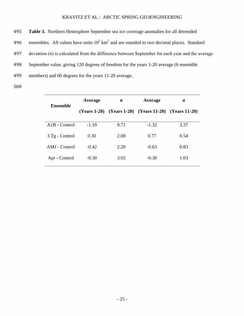
Because of the negative radiative forcing in the Arctic due to the sulfate aerosols, the loss 274

of Arctic sea ice should slow under geoengineering, with a possible re-growth of sea ice. Table 275

3 shows average values and standard deviations of Northern Hemisphere September sea ice area 276

coverage for all of the experiments. Under A1B, Arctic sea ice coverage (averaged over the 277

second decade of the simulation) is reduced from the control case by over 105 km

2 according to 278

the model results. Under 3 Tg, sea ice actually increases in areal extent. In AMJ and Apr, sea 279

ice coverage is still reduced from the control case, but not as much as in A1B. Apr appears to be 280

slightly more effective at preserving sea ice than AMJ, suggesting having a higher radiative 281

forcing in the early spring is more important to maintaining September sea ice coverage than 282

having a lower radiative forcing for a longer period of time. Of all of these values, only AMJ 283

and 3 Tg are separable by more than one standard deviation. 284

Vinnikov et al. [1999] performed long control run simulations using the GFDL model 285

[Manabe et al., 1991, 1992; Manabe and Stouffer, 1997; Haywood et al., 1997] to determine 286

whether a given Northern Hemisphere sea ice trend over a certain time interval would occur by 287

chance. Using the second decade of our simulations, with 6 ensemble members each, we can 288

compare the trends in Table 3 with their results for a trend over a 60 year period. The units 289

given in Vinnikov et al. for a trend are million square km per 10 years, so our results are directly 290

comparable by multiplying their values by 10. Converting the results of Vinnikov et al., over a 291

60 year time interval, a trend of approximately 0.5 105 km2 per 10 years will occur by chance 292

less than 10% of the time, and a trend of approximately 1.5 105 km2 per 10 years will occur by 293


- 13 -

chance less than 0.1% of the time. With the exception of the Apr ensemble, all of our 294

simulations fall within this envelope of values. Specifically, the trend of 1.32 105 km2 over 295

simulation years 11-20, which is the result of the A1B ensemble, will occur by chance less than 296

0.5% of the time. For the geoengineering experiments, the trend of 0.77 105 km2 over 297

simulation years 11-20, which is the result of the 3 Tg ensemble, will occur by chance less than 298

3% of the time, and the trend of 0.63 105 km2 over simulation years 11-20, which is the result 299

of the AMJ ensemble, will occur by chance less than 5% of the time. 300

Comparing differences between the ensembles makes the results more stark. The trend 301

difference between the 3 Tg and A1B ensembles of 2.02 105 km2 over the second decade is 302

highly unlikely to have occurred by natural climate variability. Similarly, the difference between 303

the AMJ and A1B ensembles of 0.69 105 km2 over the second decade would occur less than 304

5% of the time by natural variability, and the difference between Apr and A1B of 1.02 105 km2 305

over the second decade would occur less than 1% of the time by natural variability. Due to the 306

large standard deviations of these trends, as reported in Table 3, we are hesitant to make firm 307

conclusions from this data. However, our results would suggest that a comparison between our 308

simulations and the results of Vinnikov et al. [1999] implies geoengineering in the Arctic spring 309

will prevent some loss of sea ice compared to an A1B scenario. 310

The version of ModelE used to generate this output has a problem with the sea ice 311

module which results in a reduced climate sensitivity in the Arctic, meaning the loss of sea ice 312

under anthropogenic warming is slower than should be experienced [G. Schmidt, personal 313

communication]. The effect of this model issue on our results would be a smaller response of 314

sea ice coverage to radiative forcing than should be experienced, meaning were the issue not 315

present, sea ice loss under the A1B scenario would be greater, and the recovery of the sea ice 316


- 14 -

under geoengineering would be more pronounced. This could also have the effect of making the 317

sea ice recovery from geoengineering more statistically significant, although we are unable to 318

quantify this potential change in our results. 319

7. Discussion and Conclusions 320

We conclude that geoengineering with stratospheric aerosols in the Arctic spring, despite 321

taking advantage of the months of maximum insolation, is not as effective as year-round SO2 322

injections of the same daily rate at cooling the planet or preventing the loss of Arctic sea ice. 323

However, each of our spring injection experiments shows cooler temperatures and more Arctic 324

sea ice than the A1B ensemble, which are two of the desired purposes of geoengineering. Only 325

our 3 Tg experiment shows even a slight monsoonal reduction. We argue this difference 326

between our results and those of Robock et al. [2008] is due to model tuning, but we are unable 327

to conclude whether geoengineering would indeed cause a monsoonal disruption. According to 328

our model results, if the primary goal of a geoengineering policy were to save the Arctic sea ice, 329

the spring injection scenarios presented here appear to be well suited to satisfying this policy. 330

The effectiveness of AMJ and Apr could be increased by magnifying the summer 331

radiative forcing to levels seen in 3 Tg. This could be accomplished by increasing the daily rate 332

of injection or, in analogy to Kravitz and Robock [2010], extending the time of year over which 333

the injections occur. This latter means is potentially the more effective one, as it will counteract 334

some of the aerosol deposition that occurs throughout the year, and it will allow for aerosol 335

creation during months that have sunlight but do not experience maximum insolation. In either 336

case, this would involve an increase in the annual amount of SO2 injected, although the total 337

amount would still be less than year-round injection. Based on our findings here and the results 338

of Kravitz and Robock, we postulate a near optimal injection scenario would be at the same daily 339


- 15 -

rate as the 3 Tg experiment, but with daily injections over the 6 month period of mid-March 340

through mid-September. However, further experimentation is needed to assess this hypothesis. 341

This study has a strong need for follow-up and improvement upon the results presented 342

here. First, to make the results comparable to those of Robock et al. [2008], the spring injection 343

experiments could be run with the version of the model prior to tuning to analyze precipitation 344

effects of geoengineering. However, the model was tuned to resolve a strong temperature trend, 345

and as we show, this tuning affected the model results. The model’s accuracy in resolving 346

precipitation and cloud coverage appears to agree better with observations as a result of the 347

tuning, but these fields are too different from the observations to conclusively assert that tuning 348

improved the model output. Moreover, geoengineering simulations of a similar nature need to be 349

conducted by multiple modeling groups to conclusively determine whether monsoonal disruption 350

is a robust feature of geoengineering. The Geoengineering Model Intercomparison Project 351

(GeoMIP) [Kravitz et al., 2010b] has placed this as one of its priorities, so this question may 352

soon be resolved. Second, this same study could be repeated on a different version of the model 353

in which the sea ice issue has been resolved in order to verify our hypotheses about how it 354

affected our results. We could additionally extend our runs past 2026 to obtain better statistical 355

significance. 356

Finally, Heckendorn et al. [2009] argue the aerosol size we used in our study is likely 357

much smaller than the aerosol size that would actually result from stratospheric geoengineering. 358

Using a more representative size would likely require larger injection amounts, as the scattering 359

efficiency and aerosol lifetime would both be reduced. However, since the aerosol layer in the 360

spring injection runs is replenished every year (Figure 2), perhaps the results of Heckendorn et 361

al. would not apply to these experiments, but would only apply to year-round injection scenarios. 362


- 16 -

Although this study is part of an investigation into the optimal means by which the 363

climate could be geoengineered, we can still find many reasons why geoengineering may not be 364

a good idea [e.g., Robock, 2008]. Also, compared to some large volcanic eruptions, for which 365

the current observation system already has large gaps [Kravitz et al., 2010a], the amount of 366

climate interference suggested in this paper is small and would be difficult to observe and 367

analyze [Robock et al., 2010]. 368

369

Acknowledgments. We thank Georgiy Stenchikov for his help in the initial stages of this study 370

and Gavin Schmidt for detailed description of the Arctic climate sensitivity issue in ModelE. 371

Model development and computer time at Goddard Institute for Space Studies are supported by 372

National Aeronautics and Space Administration climate modeling grants. This work is 373

supported by NSF grant ATM-0730452. 374

375


- 17 -

References 376

Caldeira, K. and L. Wood (2008), Global and Arctic climate engineering: Numerical model 377

studies, Phil. Trans. Royal Soc. A, 366(1882), 4039-4056, doi:10.1098/rsta.2008.0132. 378

Crutzen, P. (2006), Albedo enhancement by stratospheric sulfur injections: A contribution to 379

resolve a policy dilemma? Climatic Change, 77, 211-219. 380

Hansen, J., et al. (2005), Efficacy of climate forcings, J. Geophys. Res., 110, D18104, 381

doi:10.1029/2005JD005776. 382

Haywood, J. M., R. J. Stouffer, R. T. Wetherald, S. Manabe, and V. Ramaswamy (1997), 383

Transient response of a coupled model to estimated changes in greenhouse gas and sulfate 384

concentrations, Geophys. Res. Lett., 24(11), 1335-1338. 385

Heckendorn, P., D. Weisenstein, S. Fueglistaler, B. P. Luo, E. Rozanov, M. Schraner, L. W. 386

Thomason, and T. Peter (2009), The impact of geoengineering aerosols on stratospheric 387

temperature and ozone, Env. Res. Lett., 4, 045108, doi:10.1088/1748-9326/4/4/045108. 388

IPCC (2001), Climate Change 2001: The Scientific Basis. Contribution of Working Group I to 389

1006 the Third Assessment Report of the Intergovernmental Panel on Climate Change, 390

Houghton, J. T., Y. Ding, D. J. Griggs, M. Noguer, P. J. van der Linden, X. Dai, K. Maskell, 391

and C.A. Johnson, Eds., (Cambridge University Press, Cambridge, United Kingdom and New 392

York, NY, USA), 881 pp. 393

IPCC (2007), Climate Change 2007: The Physical Science Basis. Contribution of Working 394

Group I to the Fourth Assessment Report of the Intergovernmental Panel on Climate 395

Change, S. Solomon, D. Qin, M. Manning, Z. Chen, M. Marquis, K. B. Averyt, M. Tignor 396

and H. L. Miller, Eds., (Cambridge University Press, Cambridge, United Kingdom and New 397

York, NY, USA), 996 pp. 398


- 18 -

Jones, A., J. Haywood, O. Boucher, B. Kravitz, and A. Robock (2010), Geoengineering by 399

stratospheric SO2 injection: results from the Met Office HadGEM2 climate model and 400

comparison with the Goddard Institute for Space Studies ModelE, Atmos. Chem. Phys., 10, 401

5999-6006, doi:10.5194/acp-10-5999-2010. 402

Koch, D., G. A. Schmidt, and C. V. Field (2006), Sulfur, sea salt, and radionuclide aerosols in 403

GISS ModelE, J. Geophys. Res., 111, D06206, doi:10.1029/2004JD005550. 404

Kravitz, B., A. Robock, A. Bourassa, and G. Stenchikov (2010a), Negligible climatic effects 405

from the 2008 Okmok and Kasatochi volcanic eruptions, J. Geophys. Res., 115, D00L05, 406

doi:10.1029/2009JD013525. 407

Kravitz, B. and A. Robock (2010), The climate effects of high latitude eruptions: The role of the 408

time of year, J. Geophys. Res., submitted, available at 409

http://climate.envsci.rutgers.edu/pdf/KravitzTimeOfYearSubmitted.pdf. 410

Kravitz, B., A. Robock, O. Boucher, H. Schmidt, K. E. Taylor, G. Stenchikov, and M. Schulz 411

(2010b), The Geoengineering Model Intercomparison Project (GeoMIP), Atm. Sci. Lett., 412

submitted, available at http://climate.envsci.rutgers.edu/pdf/GeoMIP17.pdf. 413

McKeen, S. A., S. C. Liu, and C. S. Kiang (1984), On the chemistry of stratospheric SO2 from 414

volcanic eruptions, J. Geophys. Res., 89(D3), 4873-4881, doi:10.1029/JD089iD03p04873. 415

Manabe, S., R. J. Stouffer, M. J. Spelman, and K. Bryan (1991), Transient Responses of a 416

Coupled Ocean–Atmosphere Model to Gradual Changes of Atmospheric CO2, Part I: Annual 417

Mean Response, J. Climate, 4, 785–818. 418

Manabe, S., M. J. Spelman, and R. J. Stouffer (1992), Transient Responses of a Coupled Ocean-419

Atmosphere Model to Gradual Changes of Atmospheric CO2, Part II: Seasonal Response, J. 420

Climate, 5, 105–126. 421

http://climate.envsci.rutgers.edu/pdf/KravitzTimeOfYearSubmitted.pdf


- 19 -

Manabe, S. and R. J. Stouffer (1997), Climate variability of a coupled ocean-atmosphere-land 422

surface model : Implication for the detection of global warming, BAMS, 78(6), 1177-1185. 423

Oman, L., A. Robock, G. L. Stenchikov, G. A. Schmidt, and R. Ruedy (2005), Climatic response 424

to high-latitude volcanic eruptions, J. Geophys. Res., 110, D13103, 425

doi:10.1029/2004JD005487. 426

Oman, L., A. Robock, G. L. Stenchikov, T. Thordarson, D. Koch, D. T. Shindell, and C. Gao 427

(2006a), Modeling the distribution of the volcanic aerosol cloud from the 1783-1784 Laki 428

eruption, J. Geophys. Res., 111, D12209, doi:10.1029/2005JD006899. 429

Oman, L., A. Robock, G. L. Stenchikov, and T. Thordarson (2006b), High-latitude eruptions cast 430

shadow over the African monsoon and the flow of the Nile, Geophys. Res. Lett., 33, L18711, 431

doi:10.1029/2006GL027665. 432

Rasch, P. J., S. Tilmes, R. P. Turco, A. Robock, L. Oman, C.-C. Chen, G. L. Stenchikov, and R. 433

R. Garcia (2008), An overview of geoengineering of climate using stratospheric sulfate 434

aerosols, Phil. Trans. Royal Soc. A, 366, 4007-4037, doi:10.1098/rsta.2008.0131. 435

Robock, A., T. Adams, M. Moore, L. Oman, and G. Stenchikov (2007), Southern hemisphere 436

atmospheric circulation effects of the 1991 Mount Pinatubo eruption, Geophys. Res. Lett., 34, 437

L23710, doi:10.1029/2007GL031403. 438

Robock, A. (2008), 20 reasons why geoengineering may be a bad idea, Bull. Atomic Scientists, 439

64, No. 2, 14-18, 59, doi:10.2968/064002006. 440

Robock, A., L. Oman, and G. Stenchikov (2008), Regional climate responses to geoengineering 441

with tropical and Arctic SO2 injections, J. Geophys. Res., 113, D16101, doi:10.1029/ 442

2008JD010050. 443


- 20 -

Robock, A., A. Marquardt, B. Kravitz, and G. Stenchikov (2009), Benefits, risks, and costs of 444

stratospheric geoengineering, Geophys. Res. Lett., 36, L19703, doi:10.1029/2009GL039209. 445

Robock, A., M. Bunzl, B. Kravitz, and G. Stenchikov (2010), A test for geoengineering?, 446

Science, 327(5965), 530-531, doi:10.1126/science.1186237. 447

Rossow, W. B., A. W. Walker, D. E. Benschel, and M. D. Roiter (1996), International Satellite 448

Cloud Climatology Project (ISCCP) documentation of new cloud datasets, WMO/TD-No. 449

737, World Meteorological Organization, 115 pp., available at 450

http://isccp.giss.nasa.gov/pub/documents/d-doc.eps.gz 451

Rudolf, B., and U. Schneider (2005), Calculation of gridded precipitation data for the land-452

surface using in-situ gauge observations, Proceedings of the 2nd Workshop of the 453

International Precipitation Working Group IPWG, Monterey, California, October 2004, 231-454

247. 455

Russell, G. L., J. R. Miller, and D. Rind (1995), A coupled atmosphere-ocean model for transient 456

climate change, Atmos.-Ocean, 33, 683-730. 457

Schmidt, G. A., et al. (2006), Present day atmospheric simulations using GISS ModelE: 458

Comparison to in situ, satellite and reanalysis data, J. Climate, 19, 153-192. 459

Schneider, U., T. Fuchs, A . Meyer-Christoffer, and B. Rudolf (2008), Global precipitation 460

analysis of the GPCC, 12 pp., available at ftp://ftp-461

anon.dwd.de/pub/data/gpcc/PDF/GPCC_intro_products_2008.pdf 462

Stothers, R. B. (1997), Stratospheric aerosol clouds due to very large volcanic eruptions of the 463

early twentieth century: Effective particle sizes and conversion from pyrheliometric to visual 464

optical depth, J. Geophys. Res., 102(D5), 6143-6151. 465

http://isccp.giss.nasa.gov/pub/documents/d-doc.eps.gz

ftp://ftp-anon.dwd.de/pub/data/gpcc/PDF/GPCC_intro_products_2008.pdf

ftp://ftp-anon.dwd.de/pub/data/gpcc/PDF/GPCC_intro_products_2008.pdf


- 21 -

Tang, I. N. (1996), Chemical and size effects of hygroscopic aerosols on light scattering 466

coefficients, J. Geophys. Res., 101, D14, 19245-19250. 467

Trenberth, K. E., and A. Dai (2007), Effects of Mount Pinatubo volcanic eruption on the 468

hydrological cycle as an analog of geoengineering, Geophys. Res. Lett., 34, L15702, 469

doi:10.1029/2007GL030524. 470

Vinnikov, K. Y., et al. (1999), Global warming and Northern Hemisphere sea ice extent, Science, 471

286, 1934, doi:10.1126/science.286.5446.1934. 472

Wigley, T. M. L. (2006), A combined mitigation/geoengineering approach to climate 473

stabilization, Science, 314, 5798, 452-454, doi:10.1126/science.1131728. 474


- 22 -

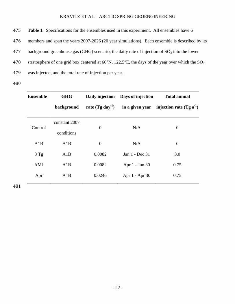
Table 1. Specifications for the ensembles used in this experiment. All ensembles have 6 475

members and span the years 2007-2026 (20 year simulations). Each ensemble is described by its 476

background greenhouse gas (GHG) scenario, the daily rate of injection of SO2 into the lower 477

stratosphere of one grid box centered at 66°N, 122.5°E, the days of the year over which the SO2 478

was injected, and the total rate of injection per year. 479

480

Ensemble GHG

background

Daily injection

rate (Tg day-1

)

Days of injection

in a given year

Total annual

injection rate (Tg a-1

)

Control

constant 2007

conditions

0 N/A 0

A1B A1B 0 N/A 0

3 Tg A1B 0.0082 Jan 1 - Dec 31 3.0

AMJ A1B 0.0082 Apr 1 - Jun 30 0.75

Apr A1B 0.0246 Apr 1 - Apr 30 0.75

481


- 23 -

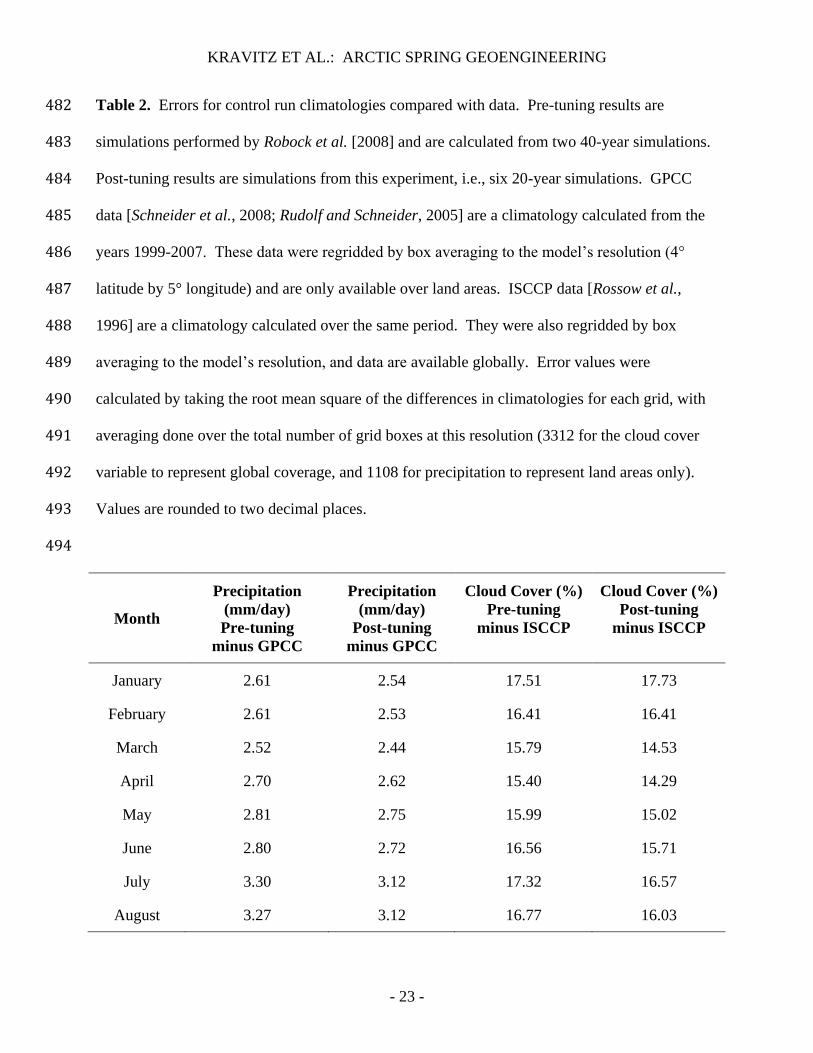
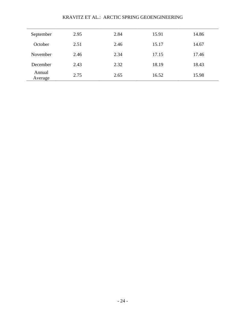
Table 2. Errors for control run climatologies compared with data. Pre-tuning results are 482

simulations performed by Robock et al. [2008] and are calculated from two 40-year simulations. 483

Post-tuning results are simulations from this experiment, i.e., six 20-year simulations. GPCC 484

data [Schneider et al., 2008; Rudolf and Schneider, 2005] are a climatology calculated from the 485

years 1999-2007. These data were regridded by box averaging to the model’s resolution (4° 486

latitude by 5° longitude) and are only available over land areas. ISCCP data [Rossow et al., 487

1996] are a climatology calculated over the same period. They were also regridded by box 488

averaging to the model’s resolution, and data are available globally. Error values were 489

calculated by taking the root mean square of the differences in climatologies for each grid, with 490

averaging done over the total number of grid boxes at this resolution (3312 for the cloud cover 491

variable to represent global coverage, and 1108 for precipitation to represent land areas only). 492

Values are rounded to two decimal places. 493

494

Month

Precipitation

(mm/day)

Pre-tuning

minus GPCC

Precipitation

(mm/day)

Post-tuning

minus GPCC

Cloud Cover (%)

Pre-tuning

minus ISCCP

Cloud Cover (%)

Post-tuning

minus ISCCP

January 2.61 2.54 17.51 17.73

February 2.61 2.53 16.41 16.41

March 2.52 2.44 15.79 14.53

April 2.70 2.62 15.40 14.29

May 2.81 2.75 15.99 15.02

June 2.80 2.72 16.56 15.71

July 3.30 3.12 17.32 16.57

August 3.27 3.12 16.77 16.03


- 24 -

September 2.95 2.84 15.91 14.86

October 2.51 2.46 15.17 14.67

November 2.46 2.34 17.15 17.46

December 2.43 2.32 18.19 18.43

Annual

Average 2.75 2.65 16.52 15.98


- 25 -

Table 3. Northern Hemisphere September sea ice coverage anomalies for all detrended 495

ensembles. All values have units 105 km

2 and are rounded to two decimal places. Standard 496

deviation (σ) is calculated from the difference between September for each year and the average 497

September value, giving 120 degrees of freedom for the years 1-20 average (6 ensemble 498

members) and 60 degrees for the years 11-20 average. 499

500

Ensemble

Average

(Years 1-20)

σ

(Years 1-20)

Average

(Years 11-20)

σ

(Years 11-20)

A1B - Control -1.19 9.71 -1.32 3.37

3 Tg - Control 0.30 2.08 0.77 0.54

AMJ - Control -0.42 2.20 -0.63 0.83

Apr - Control -0.30 3.02 -0.30 1.03


- 26 -

501

502

Figure 1. Seasonal cycle of sulfate aerosol optical depth (λ=550 nm) and surface shortwave 503

radiative forcing at the surface due to sulfate aerosols. Seasonal cycle is calculated from an 504

average of years 11-20 of the simulation. Shaded areas are ±1 standard deviation, calculated 505

from the different ensemble members (6 degrees of freedom). All values shown are Northern 506

Hemisphere averages.507


- 27 -

508

509

Figure 2. Seasonal cycle of sulfate aerosol optical depth and surface shortwave radiative forcing 510

at the surface due to sulfate aerosols. Seasonal cycle is calculated from an average of years 11-511

20 of the simulation. All plots shown are zonal averages. The Southern Hemisphere is not 512

shown, as all values are zero at those latitudes. 513


- 28 -

514

Figure 3. Globally averaged surface air temperature and precipitation due to geoengineering. 515

All values shown are running 12 month means, averaged from the current month through the 516

following 11 months (t+0 through t+11). Yellow shading shows the range of the individual 517

ensemble members of A1B minus control. Orange lines indicate ±1.96σ of a 12 month running 518

mean of the variability of the control ensemble.519


- 29 -

520

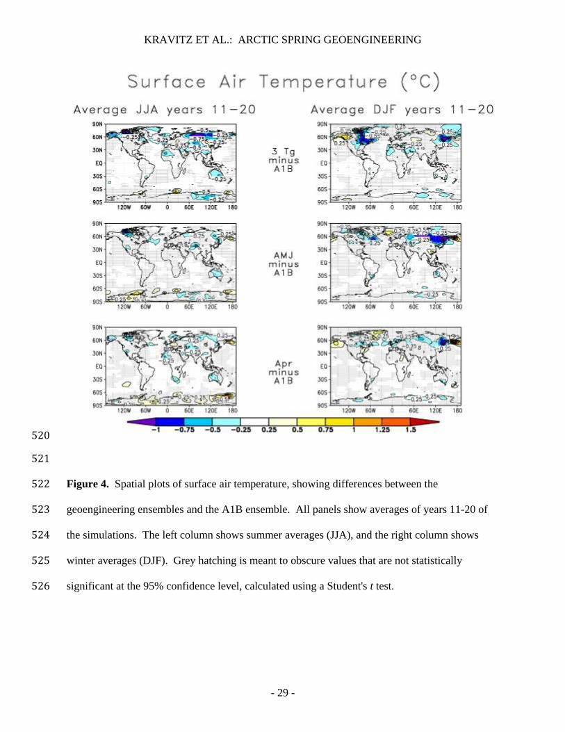
521

Figure 4. Spatial plots of surface air temperature, showing differences between the 522

geoengineering ensembles and the A1B ensemble. All panels show averages of years 11-20 of 523

the simulations. The left column shows summer averages (JJA), and the right column shows 524

winter averages (DJF). Grey hatching is meant to obscure values that are not statistically 525

significant at the 95% confidence level, calculated using a Student's t test.526


- 30 -

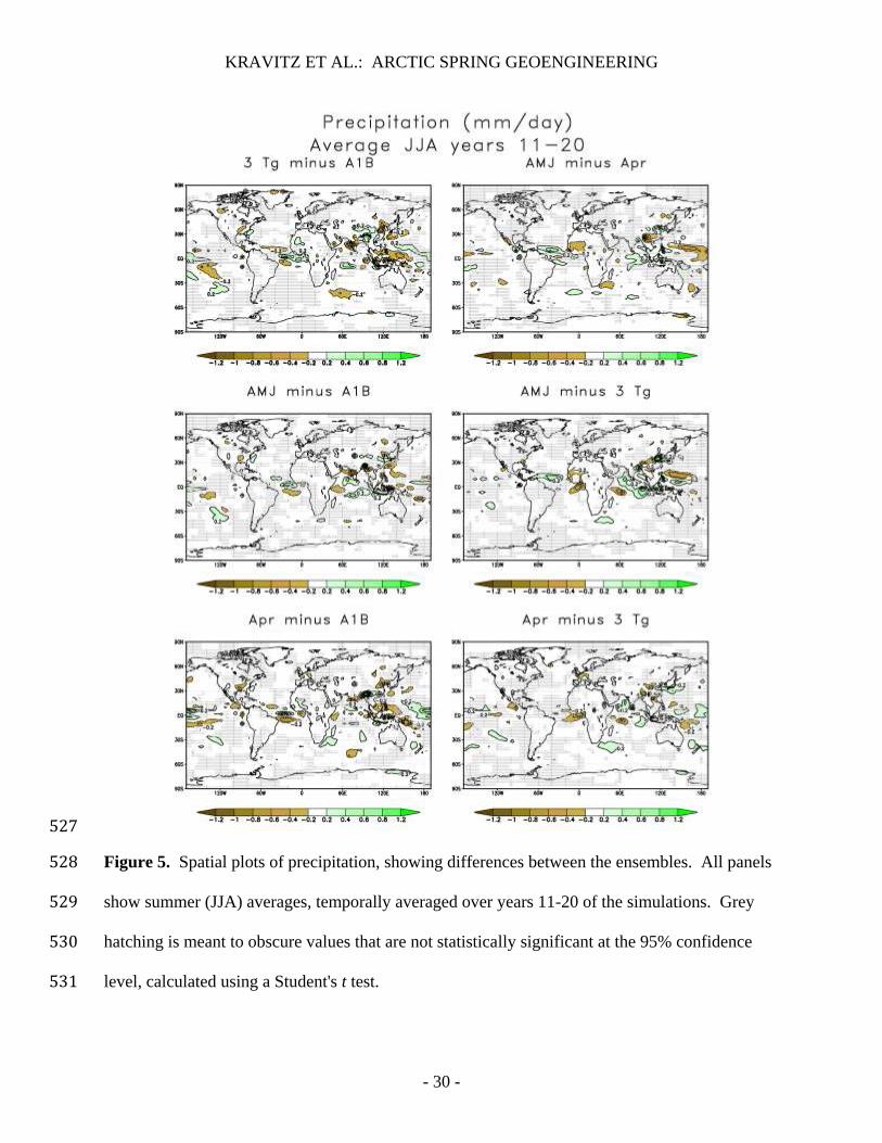
527

Figure 5. Spatial plots of precipitation, showing differences between the ensembles. All panels 528

show summer (JJA) averages, temporally averaged over years 11-20 of the simulations. Grey 529

hatching is meant to obscure values that are not statistically significant at the 95% confidence 530

level, calculated using a Student's t test.531


- 31 -

532

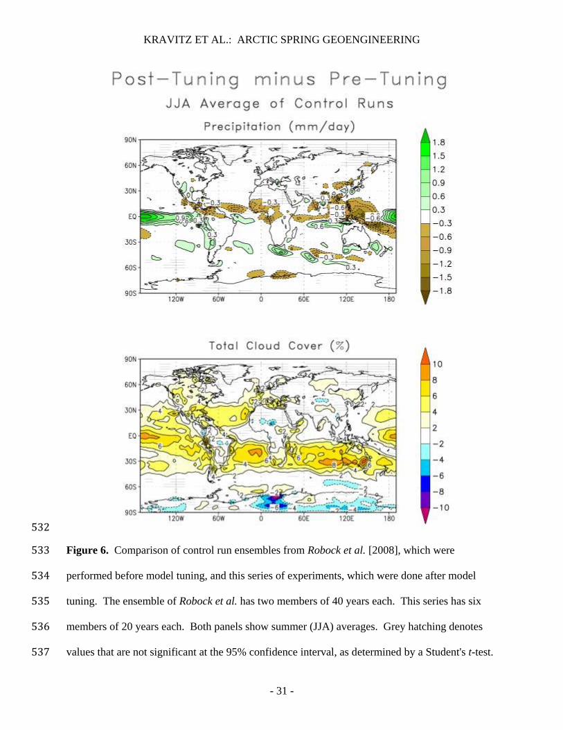
Figure 6. Comparison of control run ensembles from Robock et al. [2008], which were 533

performed before model tuning, and this series of experiments, which were done after model 534

tuning. The ensemble of Robock et al. has two members of 40 years each. This series has six 535

members of 20 years each. Both panels show summer (JJA) averages. Grey hatching denotes 536

values that are not significant at the 95% confidence interval, as determined by a Student's t-test.537


- 32 -

538

539

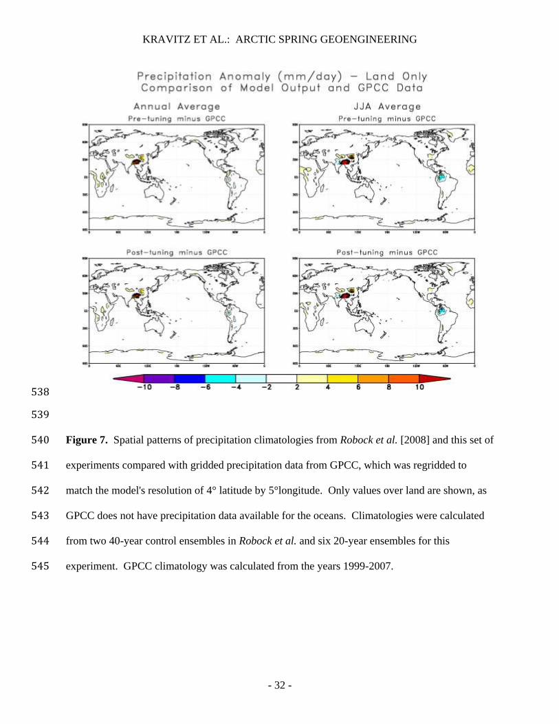
Figure 7. Spatial patterns of precipitation climatologies from Robock et al. [2008] and this set of 540

experiments compared with gridded precipitation data from GPCC, which was regridded to 541

match the model's resolution of 4° latitude by 5°longitude. Only values over land are shown, as 542

GPCC does not have precipitation data available for the oceans. Climatologies were calculated 543

from two 40-year control ensembles in Robock et al. and six 20-year ensembles for this 544

experiment. GPCC climatology was calculated from the years 1999-2007.545


- 33 -

546

547

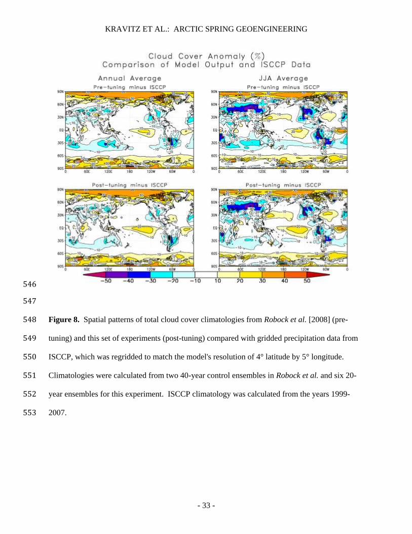
Figure 8. Spatial patterns of total cloud cover climatologies from Robock et al. [2008] (pre-548

tuning) and this set of experiments (post-tuning) compared with gridded precipitation data from 549

ISCCP, which was regridded to match the model's resolution of 4° latitude by 5° longitude. 550

Climatologies were calculated from two 40-year control ensembles in Robock et al. and six 20-551

year ensembles for this experiment. ISCCP climatology was calculated from the years 1999-552

2007. 553

KRAVITZ ET AL.: ARCTIC SPRING GEOENGINEERINGclimate.envsci.rutgers.edu/pdf/ArcticSpring.pdf ·...

Documents

Transcript of KRAVITZ ET AL.: ARCTIC SPRING GEOENGINEERINGclimate.envsci.rutgers.edu/pdf/ArcticSpring.pdf ·...