KPZ equation tails for general initial data

E l e c t r o n ic

Jo

ur n a l

of

Pr

o b a b i l i t y

Electron. J. Probab. 25 (2020), article no. 66, 1–38.ISSN: 1083-6489 https://doi.org/10.1214/20-EJP467

KPZ equation tails for general initial data

Ivan Corwin* Promit Ghosal†

Abstract

We consider the upper and lower tail probabilities for the centered (by time/24) andscaled (according to KPZ time1/3 scaling) one-point distribution of the Cole-Hopfsolution of the KPZ equation when started with initial data drawn from a very generalclass. For the lower tail, we prove an upper bound which demonstrates a crossoverfrom super-exponential decay with exponent 3 in the shallow tail to an exponent 5/2in the deep tail. For the upper tail, we prove super-exponential decay bounds withexponent 3/2 at all depths in the tail.

Keywords: KPZ equation; KPZ line ensemble; Brownian Gibbs property.AMS MSC 2010: 60K35.Submitted to EJP on July 19, 2019, final version accepted on May 17, 2020.Supersedes arXiv:1810.07129.

1 Introduction

In this paper we consider the following question: How does the initial data foran SPDE affect the statistics of the solution at a later time? Namely, we considerthe Kardar-Parisi-Zhang (KPZ) equation (or equivalently, the stochastic heat equation(SHE)) and probe the lower and upper tails of the centered (by time/24) and scaled(by time1/3) one-point distribution for the solution at finite and long times. Our mainresults (Theorems 1.2 and 1.4) show that within a very large class of initial data, thetail behavior for the KPZ equation does not change in terms of the super-exponentialdecay rates and at most changes in terms of the coefficient in the exponential. Theseresults are the first tail bounds for general initial data which capture the correct decayexponents and which respect the long-time scaling behavior of the solution.

In order to state our results, let us recall the KPZ equation, which is formally writtenas

∂TH(T,X) =1

2∂2XH(T,X) +

1

2(∂XH(T,X))2 + ξ(T,X), H(0, X) = H0(X).

*Columbia University, Department of Mathematics, 2990 Broadway, New York, NY 10027, USA.E-mail: [email protected]

†Columbia University, Department of Statistics, 1255 Amsterdam, New York, NY 10027, USA.E-mail: [email protected]

http://www.imstat.org/ejp/

https://doi.org/10.1214/20-EJP467

http://arXiv.org/abs/1810.07129

mailto:[email protected]

mailto:[email protected]

KPZ equation tails

Here, ξ is the space-time white noise, whose presence (along with the non-linearity)renders this equation ill-posed. A proper definition of the solution of the KPZ equationcomes from the Cole-Hopf transform by which we define

H(T,X) := logZ(T,X) (1.1)

where Z(T,X) is the unique solution of the well-posed SHE

∂TZ(T,X) =1

2∂2XZ(T,X) + Z(T,X)ξ(T,X), Z0(X) = eH0(X).

Note that the logarithm in (1.1) is defined since Z(T,X) is almost-surely strictly positivefor all T > 0 and X ∈ R [Mue91]. We refer to [Qua12, Cor12, Hai13] for more detailsabout the KPZ equation and the SHE and their relation to random growth, interactingparticle systems, directed polymers and other probabilistic systems (see also [Mol,Kho14, BC95, BC17, Com17]).

In this paper, we consider very general initial data as now describe.

Definition 1.1. Fix ν ∈ (0, 1) and C, θ, κ,M > 0. A measurable function f : R →R ∪ −∞ satisfies Hyp(C, ν, θ, κ,M) if:

(1) f(y) ≤ C +ν

22/3y2, ∀y ∈ R, (1.2)

(2) there exists a subinterval I ⊂ [−M,M ] with |I| = θ such that

f(y) ≥ −κ, ∀y ∈ I. (1.3)

For a measurable function f : R→ R ∪ −∞, and T > 0 consider the solution to theKPZ equation with initial data H0 chosen such that

T−13H0

((2T )

23 y)

= f(y). (1.4)

We consider the KPZ equation with this initial data and run until time1 T . Namely, let

hfT (y) :=H(2T, (2T )

23 y)

+ T12 −

23 log(2T )

T13

. (1.5)

Our first main result (Theorem 1.2) provides an upper bound on the lower tail thatholds uniformly over f ∈ Hyp(C, ν, θ, κ,M), and T > 1. The proof of this and our othermain results are deferred to the later sections of the paper.

Theorem 1.2. Fix any ε, δ ∈ (0, 13 ), C,M, θ > 0, ν ∈ (0, 1), and T0 > 0. There exist

s0 = s0(ε, δ, C,M, θ, ν, T0) and K = K(ε, δ, T0) > 0 such that for all s ≥ s0, T ≥ T0, andf ∈ Hyp(C, ν, θ, κ,M) (recall hfT (y) is defined in (1.4) and (1.5)),

P(hfT (0) ≤ −s

)≤ e−T

1/3 4(1−ε)s5/215π + e−Ks

3−δ−εsT 1/3

+ e−(1−ε)s3

12 . (1.6)

Remark 1.3. There are three regions of the lower tail (see I, II, and III in Figure1). In each region (and for T large) a different one of the three terms on the r.h.s.of (1.6) becomes active. For instance, for region I when s T 2/3, the largest termin our bound is the first term in the r.h.s. of (1.6). Likewise, the middle term in ther.h.s. of (1.6) is active in region II and the last term in region III. We presently lack amatching lower bound for the lower tail probability. This is known for only the narrowwedge (see Proposition 1.10). See Section 1.3 for some discussion regarding physicsliterature related to this tail. Let us also note that one can get similar bound as in (1.6)

1Notice that the initial data and time horizon are both dependent on T . This allows for a much wider classof initial data which are adapted to the KPZ fixed point scaling.

EJP 25 (2020), paper 66./38




KPZ equation tails

I II III IV

Figure 1: Schematic plot of the density (top) and log density (bottom) of hfT (0). Lettings denote the horizontal axis variable, there are four regions which display differentbehaviors. Region I (deep lower tail, when s −T 2/3): the log density has power lawdecay with exponent 5/2. Region II (shallow lower tail, when −T 2/3 s 0): the logdensity has power law decay with exponent 3. Region III (center, when s ≈ 0): thedensity depends on initial data as predicted by the KPZ fixed point. Region IV (upper tail,when s 0): the log density has power law decay with exponent 3/2. The universality ofthe power law exponents (in regions I, II and IV ) for general initial data constitutes themain contribution of this paper.

on P(hfT (y) ≤ −s

)when y 6= 0. This is explained in Section 1.1. Finally, observe that

two important choices of initial data — narrow wedge and Brownian motion — do not fitinto this class2. The narrow wedge result is in fact a building block for the proof of thisresult, while Brownian follows as a fairly easy corollary (see Section 1.2).

Our second main result pertains to the upper tail and shows upper and lower boundswhich hold uniformly over f ∈ Hyp(C, ν, θ, κ,M), and T > π.

Theorem 1.4. Fix any ν ∈ (0, 1) and C, θ, κ,M > 0. For any T0 > 0, there exists0 = s0(C, ν, θ, κ,M, T0) > 0, c1 = c1(T0) > c2 = c2(T0) > 0 such that for all s ≥ s0, T > T0

and f ∈ Hyp(C, ν, θ, κ,M),

e−c1s3/2

≤ P(hfT (0) ≥ s

)≤ e−c2s

3/2

. (1.7)

We may further specify values of c1 and c2 for which (1.7) holds, provided we assumeT0 > π. In that case, for any ε, µ ∈ (0, 1

2 ), there exists s0 = s0(ε, µ, C, ν, θ, κ,M, T0) > 0

such that for all s ≥ s′0, T ≥ T0, and f ∈ Hyp(C, ν, θ, κ,M), (1.7) holds with the followingchoices for c1 > c2:

(i) If s0 ≤ s < 18ε

3(1 − 2µ3 )−1T

23 then we may take c1 = 8

3 (1 + µ)(1 + ε) and c2 =√

23 (1− µ)(1− ε).

(ii) If s ≥ maxs0,916ε−2(1 − 2µ

3 )−1T23 then we may take c1 = 8

√3(1 + µ)(1 + ε) and

c2 =√

23 (1− µ)(1− ε).

(iii) If maxs0,18ε

3(1 − 2µ3 )−1T

23 ≤ s ≤ maxs0,

916ε−2(1 − 2µ

3 )−1T23 then we may take

c1 = 29/2ε−3(1 + µ) and c2 =√

23 (1− µ)ε.

2The flat initial data is in the class and arises from f ≡ 0.

EJP 25 (2020), paper 66./38




KPZ equation tails

Remark 1.5. In Theorems 1.11 and 1.14, we prove similar results for narrow wedgeand Brownian initial data. The upper and lower bounds on the constants c1 and c2 arenot optimal. In fact, it is not clear to us how the initial data translates to the optimalvalue of c1 or c2. There, however, some predictions in the physics literature – see Section1.3. The condition T0 > π assumed in the second part of Theorem 1.4 could be replacedby an arbitrary lower bound, though the resulting conditions on s, c1 and c2 would needto change accordingly. This value π turns out to work well in the computations leadingto this result; in particular see (4.19).

1.1 Proof sketch

The fundamental solution to the SHE Znw(T,X) corresponds to delta initial dataZ0(X) = δX=0. For any positive T , this results in a strictly positive solution, hence thecorresponding KPZ equation solution is well-defined for T > 0 and this initial data istermed narrow wedge since in short time Z(T,X) is well-approximated by the Gaussian

heat-kernel whose logarithm is a very thin parabola X2

2T .

Definition 1.6 (Cole-Hopf Transform). The Cole-Hopf transform of Znw(T,X) is denotedhere by Hnw(T,X) := logZnw(T,X). We further define a scaled and centered version ofthis as

ΥT (y) :=Hnw(2T, (2T )

23 y) + T

12

T13

. (1.8)

The proof of our main results relies upon a combination of three ingredients: (1) lowertail bounds for the narrow wedge initial data recently proved in [CG], (2) Gibbsian lineensemble techniques applied to the KPZ line ensemble [CH16], and (3) explicit integralformulas for moments of the SHE with delta initial data. Now, we give an overview of ourproofs. A more involved discussion of the KPZ line ensemble is contained in Section 2.

To prove Theorem 1.2, one of our main tools is the upper and lower bound for thelower tail of the one point distribution of the narrow wedge solution of the KPZ equationgiven in Proposition 1.10. However, to use this result, we need a connection betweenthe solution of the KPZ equation under general initial conditions and the narrow wedgesolution. This connection is made through the following identity (which follows from theFeynman-Kac formula) which represents the one point distribution of the KPZ equationstarted from H0 as a convolution between the spatial process ΥT (·) and the initial dataH0(·).

Proposition 1.7 (Lemma 1.18 of [CH16]). For general initial data H0(·) := H(0, ·) andfor a fixed pair T > 0 and X ∈ R, the Cole-Hopf solution H(T,X) of the KPZ equationsatisfies

H(2T,X)d= log

(∫ ∞−∞

eHnw(2T,Y )+H0(X−Y )dY

)d= − T

12+ log

(∫ ∞−∞

eT13 ΥT ((2T )−

13 Y )+H0(X−Y )dY

).

Furthermore, for H0 as in (1.4), we have

H(2T, (2T )13X) + T

12 −23 log(2T )

T13

d=

1

T13

log(∫ ∞−∞

eT13

(ΥT (Y )+f(X−Y )

)dY). (1.9)

To employ this identity, we need tail bounds for the entire spatial process ΥT (·).Presently, exact formulas amenable to rigorous asymptotics are only available for one-point tail probabilities, and not multi-point. However, by using the Gibbs property for

EJP 25 (2020), paper 66./38




KPZ equation tails

the KPZ line ensemble (introduced in [CH16] and recalled here in Section 2) we will beable to extend this one-point tail control to the entire spatial process. Working with theGibbs property is a central technical aspect of our present work and forms the backboneof the proof of Theorem 1.2.

Besides the KPZ line ensemble, another helpful property of the narrow wedge KPZsolution is the stationarity of the spatial process ΥT (·) after a parabolic shift.

Proposition 1.8 (Proposition 1.4 of [ACQ11]). The one point distribution of ΥT (y)+ y2

22/3

does not depend on the value of y.

The proof of Theorem 1.4 shares a similar philosophy with that of Theorem 1.2. Wefirst prove an upper (as Theorem 1.11) and a lower bound for the upper tail probabilityof ΥT (0). The proof of Theorem 1.11 employs a combination of the one-point Laplacetransform formula (see Proposition 4.5) and moment formulas (see the proof of Lemma4.1) for Znw.

The rest of the proof of Theorem 1.4 is based on the Gibbs property of the KPZline ensemble and the FKG inequality of the KPZ equation. The FKG inequality of theKPZ equation is, for example (as shown in [CQ13, Proposition 1]) a consequence of thepositive associativity of its discrete analogue, the asymmetric simple exclusion process(ASEP).

Proposition 1.9 (Proposition 1 of [CQ13]). Let H be the Cole-Hopf solution to KPZstarted from initial data H0. Fix k ∈ Z>0. For any T1, . . . , Tk ≥ 0, X1, . . . , Xk ∈ R ands1, . . . , sk ∈ R,

P( k⋂`=1

H(T`, X`) ≤ s`

)≥

k∏`=1

P(H(T`, X`) ≤ s`

).

A simply corollary of this result is that for T1, T2 ∈ R>0, X1, X2 ∈ R and s1, s2 ∈ R,

P(H(T1, X1) > s1,H(T2, X2) > s2

)≥ P

(H(T1, X1) > s1

)P(H(T2, X2) > s2

). (1.10)

1.2 Narrow wedge and Brownian initial data results

Neither narrow wedge nor two-sided Brownian initial data belongs to the class offunctions in Definition 1.1. We record here the analogues of Theorems 1.2 and 1.4 forthese two cases. As mentioned in the last section, the one point tail results for thenarrow wedge solution are important inputs to the proof of Theorems 1.2 and 1.4. Werecall these below.

Proposition 1.10 (Theorem 1.1 of [CG]). Fix ε, δ ∈ (0, 13 ) and T0 > 0. Then, there exist

s0 = s0(ε, δ, T0), K1 = K1(ε, δ, T0) > 0, K2 = K2(T0) > 0 such that for all s ≥ s0 andT ≥ T0,

P(ΥT (0) ≤ −s) ≤ e−T1/3 4s5/2(1−ε)

15π + e−K1s3−δ−εsT 1/3

+ e−(1−ε)s3

12 (1.11)

and, P(ΥT (0) ≤ −s) ≥ e−T1/3 4s5/2(1+ε)

15π + e−K2s3

.

Our general initial data results also rely upon upper and lower bounds on the uppertail probability of ΥT (·) which are, in fact, new (see Section 1.3 for a discussion ofprevious work).

Theorem 1.11. For any T0 > 0, there exist s0 = s0(T0) > 0 and c1 = c1(T0) > c2 =

c2(T0) > 0 such that for all s ≥ s0 and T > T0

e−c1s3/2

≤ P(ΥT (0) ≥ s) ≤ e−c2s3/2

. (1.12)

EJP 25 (2020), paper 66./38




KPZ equation tails

We may further specify values of c1 and c2 for which (1.12) holds, provided we assumeT0 > π. In that case, for any ε ∈ (0, 1

2 ), there exists s0 = s0(ε, T0) > 0 such that for alls ≥ s0 and T ≥ T0, (1.12) holds with the following choices for c1 > c2:

(i) If s0 ≤ s < 18ε

2T23 then we may take c1 = 4

3 (1 + ε) and c2 = 43 (1− ε).

(ii) If s ≥ maxs0,916ε−2T

23 then we may take c1 = 4

√3(1 + ε) and c2 = 4

3 (1 − ε).Furthermore, for c1 = 4

3 (1 + ε) there exists a sequence snn≥1 with sn → ∞ as

n→∞ such that P(ΥT > sn) > e−c1s3/2n for all n.

(iii) If maxs0,18ε

2T23 ≤ s ≤ maxs0,

916ε−2T

23 then we may take c1 = 27/2ε−3 and

c2 = 43ε.

Remark 1.12. Part (i) of Theorem 1.11 shows that P(ΥT (0) > s) is close to exp(−4s32 /3)

when s T23 . This is in agreement with the fact that the tail probabilities of ΥT (0)

should be close to the tails of the Tracy-Widom GUE distribution as T increases to∞. Part (ii) of Theorem 1.11 shows that the upper bound to P(ΥT (0) > s) is closeexp(−4s

32 /3) when s T

23 . We also have some lower bound which is not tight. However,

part (ii) further tells that the lower bound for P(ΥT (0) > s) cannot differ much fromexp(−4s

32 /3) for all large s. In the regime s = O(T

23 ), we do not have tight upper and

lower bounds in (1.12), although, the decay exponent of P(ΥT (0) > s) will still be equalto 3/2.

Our next two results are about the tail probabilities for the KPZ equation with twosided Brownian motion initial data; as this initial data falls outside our class, someadditional arguments are necessary. Define HBr

0 : R→ R as HBr0 (x) := B(x) where B is

a two sided standard Brownian motion with B(0) = 0. Denote the Cole-Hopf solution ofthe KPZ equation started from this initial data HBr

0 by HBr(·, ·) and define

hBrT (y) :=

HBr(2T, (2T )23 y) + T

12 −23 log(2T )

T13

∀T > 0. (1.13)

We first state our result on the lower tail of hBrT (0).

Theorem 1.13. Fix ε, δ ∈ (0, 13 ) and T0 > 0. There exist s0 = s0(ε, δ, T0) and K =

K(ε, δ, T0) > 0 such that for all s ≥ s0 and T ≥ T0,

P(hBrT (0) ≤ −s

)≤ e−T

1/3 4(1−ε)s5/215π + e−Ks

3−δ−εsT 1/3

+ e−(1−ε)s3

12 . (1.14)

Our last result of this section is about the upper tail probability of hBrT (0).

Theorem 1.14. Fix ε, µ ∈ (0, 12 ) and T0 > 0. Then, there exists s0 = s0(ε, µ, T0) such that

for all s ≥ s0 and T ≥ T0,

e−c1s3/2

≤ P(hBrT (0) > s

)≤ e−c2s

3/2

+ e− 1

9√

3(µs)3/2

where c1 > c2 depend on the values of ε, µ and T0 as described in Theorem 1.4.

In Theorem 1.14, the second term of the upper bound (on the right-hand side of theequation) comes from the fact that Brownian motion is random, and the first term arisesin an analogous way as it does for deterministic initial data in Theorem 1.4.

As proved in [BCFV15, Theorem 2.17], hBrT (0) converges in law to the Baik-Rain dis-

tribution (see [BR00, FS006, IS04, PS04, BFP10]). The following corollary strengthensthe notion of that convergence and implies that the moments of hBr

T (0) converge to themoments of the limiting Baik-Rains distribution. This answers a question posed to us byJean-Dominique Deutschel (namely, that the variance converges).

EJP 25 (2020), paper 66./38




KPZ equation tails

Corollary 1.15. Let X be a Baik-Rains distributed random variable (see [BCFV15,Definition 2.16]). Then, E[et|X|] <∞ and for all t ∈ R,

E[et|h

BrT (0)|]→ E

[et|X|

], as T →∞. (1.15)

Proof. Theorems 1.13 and 1.14 show that et|hBrT (0)| is uniformly integrable. The dom-

inated convergence theorem, along with [BCFV15, Theorem 2.17] yields (1.15) andE[et|X|] < ∞.

1.3 Previous work and further directions

The study of tail probabilities for the KPZ equation and the SHE has a number ofmotivations including intermittency and large deviations. We recall some of the relevantprevious literature here and compare what is done therein to the results of this presentwork.

The first result regarding the lower tail probability of Z(T,X) the proof of its almostsure positivity by [Mue91]. Later, [MN08] investigated the lower tail of the SHE re-stricted on the unit interval with general initial data and Dirichlet boundary condition;they bounded P(logZ(T,X) ≤ −s) from above by c1 exp(−c2s

32−δ) (where c1, c2 are two

positive constants depending inexplicitly on T ). In [MF14], this upper bound was furtherimproved to c1 exp(−c2s2) for the delta initial data SHE (the constants are differentbut still depend inexplicitly on T ). Using these bounds, [CH16] demonstrated similarupper bounds on the lower tail probability of the KPZ equation under general initialdata. There are also tail bounds for the fractional Laplacian (∆α/2 with α ∈ (1, 2]) SHE.[CHN16, Theorem 1.5] generalizes the bound of [MN08] and shows an upper bound3

with exponent 2− 1/α (= 3/2 when α = 2).None of the previous SHE lower tail bounds were suitable to taking time T large.

Specifically, the constants depend inexplicitly on T and the centering by T/24 and scalingby T 1/3 were not present. Thus, as T grows, the bounds weaken significantly to thepoint of triviality. For instance, one cannot conclude tightness of the centered and scaledversion of logZ(T,X) (ΥT (X) herein) as T goes to infinity using the bounds.

The first lower tail bounds suitable to taking T large came in our previous work [CG]which dealt with the delta initial data SHE (see Proposition 1.10 herein). That resultrelied upon an identity of [BG16] (see Proposition 4.5). No analog of that identity seemsto exist for general initial data. This is why we use the KPZ line ensemble approach inour present work.

The upper tail probability of the SHE had been studied before in a number ofplaces. For instance, see [CD15, CJK13, KKX17] in regards to its connection to themoments and the intermittency property [GM90, GKM07] of the SHE. Again, there isa question of whether results are suitable to taking T large. The only such result is[CQ13, Corollary 14] which shows that for some constants c1, c2, c′1, c

′2, and s, T ≥ 1,

P(ΥT > s) ≤ c1 exp(−c′1sT 1/3) + c2 exp(−c′2s3/2). When s T23 the second bound is

active and one sees the expected 3/2 power-law in the exponent. However, as s T23 ,

the leading term above become c1 exp(−c′1sT13 ) and only demonstrates exponential decay.

Our result (Theorem 1.11) shows that c1 exp(−c′1sT13 ) is not a tight upper bound for

P(ΥT > s) in this regime of s. In fact, the 3/2 power-law is shown to be valid for all seven as T grows (with upper and lower bounds of this sort).

3In light of our results, it might natural to expect the true decay exponent is 3− 1/α. Perhaps the methodsof [MF14] can be applied to give decay at least with exponent 2. Heuristically, one may be able to see the trueexponent by using the physics weak noise theory as in, for example, [KMS16].

EJP 25 (2020), paper 66./38




KPZ equation tails

Some works have focused on the large s but fixed T upper tail, e.g. [CJK13] showedthat logP

(logZ(T,X) > s

) −s 3

2 as s → ∞ where Z(0, X) ≡ 1. These results arenot suitable for taking T and s large together. Our results (Theorems 1.4, 1.11 and1.14) provide the first upper and lower bound for the upper tail probability which arewell-adapted to taking T large. In particular, we showed that for a wide range of initialdata the exponent of the upper tail decay is always 3

2 (a result which was not provedbefore for any specific initial data). However, the constants in the exponent for ourbounds on the upper tail probability are not optimal.

It is natural to speculate on the values of these optimal coefficients. There is somediscussion of this in the physics literature (see, for example, [KMS16, HLDM+18]) basedon numerics and the weak noise theory (WNT)4. In the deep lower tail (the 5/2 exponentregion) the coefficient depends on the initial data and can be predicted using the WNTas in [KMS16]. For the shallow lower tail (the 3 exponent region) one expects (by reasonof continuity) to have a coefficient corresponding to the tail decay of the KPZ fixed pointwith the corresponding initial data. Remarkably, for the upper tail (the 3/2 exponentregion) it seem that for all deterministic initial data, the upper tail coefficient remainsthe same5. However, for Brownian initial data, the coefficient changes by a factorof 2.

There have been previous considerations of tail bounds in the direction of studyinglarge deviations for the KPZ equation (i.e., the probability that as T → ∞, logZ(T,X)

looks like cT for some constant not equal to −1/24). The speed for the upper tail andlower tail are different (the former being T and the later being T 2). The lower tail largedeviation principle has been the subject of significant study in the physics literature(see [SMP17, CGK+18, KL18a, KL18b] and references therein). Recently, [Tsa] provideda rigorous proof of the lower tail rate function. We are not aware of a rigorous proofof the (likely) simpler upper tail rate function for the KPZ equation (there is some non-rigorous predictions about this, see e.g. [LDMS16]). However, for a discrete analog (thelog-gamma polymer) and a semi-discrete analog (the O’Connell-Yor polymer) such anupper tail bound is proved in [GS13] and [Jan15] respectively.

We finally mention a few directions worth pursuing. Theorem 1.2 only provides anupper bound on the lower tail. Our KPZ line ensemble methods are able to produce alower bound, but with a worse (larger) power law. It is only for the narrow wedge initialdata that we have a tight matching lower bound. We conjecture that there should bea similarly tight upper and lower bound for the lower tail which holds true for generalinitial data. The large deviation result for the lower tail (see [SMP17, CGK+18, Tsa])is only shown for narrow wedge initial data (though there is also some work neededfor flat and Brownian initial data). It would be interesting to determine how the largedeviation rate function depends on the initial data. In fact, even for the KPZ fixed point(e.g. TASEP) this does not seem to be resolved.

Outline Section 2 reviews the KPZ line ensemble and its Gibbs property. Sections 3.1and 3.2 establish the lower tail bounds of Theorems 1.2 and 1.13 by first analyzing thenarrow wedge initial condition tails and then feeding those bounds into an argumentleveraging the Gibbs property and the convolution formula of Proposition 1.7. We provethe upper tail bounds of Theorem 1.11 in Section 4 by analyzing the moment formula(see Lemma 4.1) and the Laplace transform formula (see Proposition 4.5) of the narrowwedge solution. Sections 5.1 and 5.2 contain the proofs of (respectively) Theorems 1.4and 1.14 on the upper tail bounds under general initial data.

4The approach is to look at the KPZ equation in short time with very weak noise. This is a different problemthan looking at the deep tail, but so far the results one gets from the WNT seem to be true even in long time.

5For instance, for flat and narrow wedge initial data, the upper tail seems to have the same 4/3 coefficient.

EJP 25 (2020), paper 66./38




KPZ equation tails

2 KPZ line ensemble

This section reviews (following the work of [CH16]) the KPZ line ensemble and itsGibbs property. We use this construction in order to transfer one-point information(namely, tail bounds) into spatially uniform information for ΥT (y) (see Definition 1.6). Itis through this mechanism that we can escape the bonds of exact formulas and generalizethe conclusions of [CG] to general initial data.

Definition 2.1. Fix intervals Σ ⊂ N and Λ ⊂ R. Let X be the set of all continuousfunctions f : Σ × Λ 7→ R endowed with the topology of uniform convergence on thecompact subsets of Σ× Λ. Denote the sigma field generated by the Borel subsets of Xby C.

A Σ×Λ-indexed line ensemble L is a random variable in a probability space (Ω,B,P)

such that it takes values in X and is measurable with respect to (B, C). In simple words,L is a collection of Σ-indexed random continuous curves, each mapping Λ to R.

Fix two integers k1 ≤ k2, a < b and two vectors ~x, ~y ∈ Rk2−k1+1. A k1, . . . , k2 × (a, b)

– indexed line ensemble is called a free Brownian bridge line ensemble with the entrancedata ~x and the exit data ~y if its law, denoted here as Pk1,k2,(a,b),~x,~yfree , is that of k2 − k1 + 1

independent Brownian bridges starting at time a at points ~x and ending at time b atpoints ~y. We use the notation Ek1,k2,(a,b),~x,~yfree for the associated expectation operator.

Consider a continuous function H : [0,∞)→ R, which we call a Hamiltonian. GivenH and two measurable functions f : [0,∞) → R ∪ ∞ and g : [0,∞) → R ∪ −∞,we define a k1, . . . , k2 × (a, b) – indexed line ensemble with the entrance data ~x, the

exit data ~y, boundary data (f, g) and H to be the law of Pk1,k2,(a,b),~x,~y,f,gH on curvesLk1 , . . . ,Lk2 : [0,∞) → R which is given in terms of the following Radon-Nikodymderivative

dPk1,k2,(a,b),~x,~y,f,gH

dPk1,k2,(a,b)free

(Lk1 , . . . ,Lk2) =W

k1,k2,(a,b),~x,~yf,gH (Lk1 , . . . ,Lk2)

Zk1,k2,(a,b),~x,~y,f,gH

Wk1,k2,(a,b),~x,~y,f,gH (Lk1 , . . . ,Lk2) = exp

−

k2∑k=k1−1

∫ b

a

H(Lk1+1(u)− Lk(u)

)du

with the convention Lk1−1 = f and Lk2+1 = g. Here, the normalizing constant is given by

Zk1,k2,(a,b),~x,~y,f,gH = E

k1,k2,(a,b)free

[W

k1,k2,(a,b),~x,~y,f,gH (Lk1 , . . . ,Lk2)

]where the curves (Lk1 , . . . ,Lk2) are distributed via Pk1,k2,(a,b),~x,~yfree . Throughout this paperwe will restrict our attention to one parameter family of Hamiltonians indexed by T ≥ 0:

HT (x) := eT1/3x.

A Σ× Λ-indexed line ensemble L satisfies the H-Brownian Gibbs property if for anysubset K = k1, k1 + 1, . . . , k2 ⊂ Σ and (a, b) ⊂ Λ, one has the following distributionalinvariance

Law(L∣∣K×(a,b)

conditional on L∣∣Σ×Λ\K×(a,b)

)= P

k1,k2,(a,b),~x,~y,f,gH

where ~x = (ak1 , . . . , ak2), ~y = (bk1 , . . . , bk2) and f = Lk1−1|(a,b), g = Lk2+1 with f = −∞ ifk1 − 1 /∈ Σ and g = +∞ if k2 + 1 /∈ Σ. This is a spatial Markov property — the ensemblein a given region has marginal distribution only dependent on the boundary-values ofsaid region.

Denote the sigma field generated by the curves with indices outside K × (a, b) byFext(K × (a, b)). The random variable (a, b) is a K-stopping domain if a ≤ a, b ≥ b ∈

EJP 25 (2020), paper 66./38




KPZ equation tails

Fext(K × (a, b)). Let CK(a, b) be the set of continuous functions (fk1 , . . . , fk2) wherefi : (a, b)→ R and define

CK :=

(a, b, fk1 , . . . , fk2) : a < b and (fk1 , . . . , fk2) ∈ CK(a, b).

Denote the set of all Borel measurable functions from CK to R by B(CK). Then, aK-stopping domain (a, b) is said to satisfy the strong H-Brownian Gibbs property if forall F ∈ B(CK), following holds P-almost surely,

E[F(a, b,L

∣∣K×(a,b)

)∣∣∣Fext(K × (a, b))]

= Ek1,k2,(`,r),~x,~y,f,gH

[F (`, r,Lk1 , . . . ,Lk2)

](2.1)

where ` = a, r = b, ~x = Li(a)k2i=k1 , ~y = Li(b)k2i=k1 , f(·) = Lk1−1(·) (or +∞ if k1− 1 /∈ Σ)

and g(·) = Lk2+1(·) (or −∞ if k2 +1 /∈ Σ). On the l.h.s. of (2.1), L∣∣∣K×(a,b)

is the restriction

of the P-distributed curves and on the r.h.s. Lk1 , . . . ,Lk2 is Pk1,k2,(`,r),~x,~y,f,gH -distributed.

Remark 2.2. When k1 = k2 = 1 and (f, g) = (+∞,−∞) the measure Pk1,k2,(a,b),~x,~y,f,gH issame as the measure of a free Brownian bridge started from ~x and ended at ~y.

The following lemma demonstrates a sufficient condition under which the strongH-Brownian Gibbs property holds.

Lemma 2.1 (Lemma 2.5 of [CH16]). Any line ensemble which enjoys the H-BrownianGibbs property also enjoys the strong H-Brownian Gibbs property.

The next proposition relates the narrow wedge KPZ equation to the KPZ line ensem-ble6.

Proposition 2.3 (Theorem 2.15 of [CH16]). Fix any T > 0. Then there exists anN×R-indexed line ensemble HT = HnT (x)n∈N,x∈R satisfying the following properties:

(1) The lowest indexed curve H1T (X) is equal in distribution (as a process in X) the

Cole-Hopf solution Hnw(T,X) of KPZ started from the narrow wedge initial data.

(2) HT satisfies the H1-Brownian Gibbs property (see Definition 2.1).

(3) Define the scaled KPZ line ensemble Υ(n)T (x)n∈N,x∈R as follows

Υ(n)T (x) :=

Hn2T((2T )

13x)

+ T12

T13

.

Then, 2− 13 Υ

(n)T (x)n∈N,x∈R satisfies the H2T -Brownian Gibbs property7

The following proposition is a monotonicity result which shows that two line ensem-bles with the same index set can be coupled in such a way that if the boundary conditionsof one ensemble dominates the other, then likewise do the curves.

Proposition 2.4 (Lemmas 2.6 and 2.7 of [CH16]). Fix an interval K = k1, . . . , k2 ⊂ Σ

for some fixed positive integers k1 < k2, (a, b) ⊂ Λ for a < b and two pairs of vectors~x1, ~x2 and ~y1, ~y2 in Rk2−k1+1. Consider any two pairs of measurable functions f, f :

(a, b) → R ∪ +∞ and g, g : (a, b) → R ∪ −∞ such that f(s) ≤ f(s), g(s) ≤ g(s) for

all s ∈ (a, b) and x(k)2 ≤ x

(k)1 , y(k)

2 ≤ y(k)1 for all k ∈ K. Let Q = Q(n)(x)n∈K,x∈(a,b) and

Q = Q(n)(x)n∈K,x∈(a,b) be two K × (a, b)-indexed line ensembles in the probability

6Note, we do not require the full strength of the result proved in Theorem 2.15 of [CH16]. That result also

proves uniform over T of the local Brownian nature of the top curve Υ(1)T (x) as x varies.

7This pesky 2−13 compensates for the fact that it is missing in the denominator of Υ

(n)T (x).

EJP 25 (2020), paper 66./38




KPZ equation tails

space (Ω,B,P) and (Ω, B, P) respectively such that P equals to Pk1,k2,(a,b),~x1,~y1,f,gH and P

equals to Pk1,k2,(a,b),~x2,~y2,f ,gH . If H : [0,∞) → R is convex, then, there exists a coupling

(i.e., a common probability space upon which both measures are supported) between Pand P such that Q(j)(s) ≤ Q(j)(s) for all n ∈ K.

Let us provide the basic idea behind how we use Lemma 2.4. Note that by H-BrownianGibbs property the lowest indexed curve 2−

13 Υ

(1)T (·) of the N-indexed KPZ line ensemble

2− 13 Υ

(n)T (x)n∈N,x∈R, when restricted to the interval (a, b), has the conditional measure

P1,1,(a,b),2−

13 Υ

(1)T (a),2−

13 Υ

(1)T (b),+∞,2−

13 Υ

(2)T

H2T. On the other hand, replacing 2−

13 Υ

(2)T by −∞,

P1,1,(a,b),2−

13 Υ

(1)T (a),2−

13 Υ

(1)T (b),+∞,−∞

H2Tis the probability measure of a Brownian bridge on

the interval (a, b) with the entrance and exit data 2−13 Υ

(1)T (a) and 2−

13 Υ

(1)T (b) respectively.

Lemma 2.4 constructs a coupling between these two measures on the curve 2−13 Υ

(1)T

∣∣(a,b)

such that

P1,1,(a,b),2−

13 Υ

(1)T (a),2−

13 Υ

(1)T (b),+∞,2−

13 Υ

(2)T

H2T(A) ≤ P1,1,(a,b),2−

13 Υ

(1)T (a),2−

13 Υ

(1)T (b),+∞,−∞

H2T(A)

(2.2)

for any event A whose chance increases8 under the pointwise decrease of Υ(1)T .

In most of our applications of this idea, it is easy to find upper bounds on the r.h.s.of (2.2) using Brownian bridge calculations. Via (2.2), those bounds transfers to thespatial process Υ

(1)T (·). Since, by Proposition 2.3, this curve is equal in law to ΥT (·) (the

scaled and centered narrow wedge KPZ equation solution), these bounds in conjunctionwith the convolution formula of Proposition 1.7 embodies the core of our techniquesto generalize the tail bounds from narrow wedge to general initial data. The followinglemma is used in controlling the probabilities which arise on r.h.s. of (2.2).

Lemma 2.2. Let B(·) be a Brownian bridge on [0, L] with B(0) = x and B(L) = y. Then,

P(

inft∈[0,L]

B(t) ≤ minx, y − s)≤ e− 2s2

L . (2.3)

Proof. Due to symmetry, we may assume minx, y = y. Note that τ = mint ∈ [0, 1] :

B(t) ≤ y is a stopping time for the natural filtration of B(·). Thanks to the resamplinginvariance property of the Brownian bridge measure, B(t)t∈[τ,L] conditioned on thesample paths outside the interval (τ, L) is again distributed as a Brownian bridge withB(τ) = B(L) = y. Now, applying [KS91, (3.40)] (see also Lemma 2.11 of [CH16]), we get

P(

inft∈(τ,L]

B(t) ≤ minx, y − s∣∣∣F([0, τ ])

)= e−

2s2

(L−τ) . (2.4)

Here, F([0, τ ]) denotes the natural filtration of Bt∈[0,L] stopped at time τ . Taking

expectation of (2.4) with respect to the σ-algebra Fτ and noting e−2s2

(L−τ) ≤ e− 2s2

L yields(2.3).

It is worth noting that Proposition 4.3.5.3 of [JYC09] contains an exact formulas forthe left hand side of (2.3). The next result (which follows from [GT11, (3.14)]) is used inTheorem 1.14.

Lemma 2.3. Let B(·) be a two-sided standard Brownian motion with B(0) = 0. Then,for any given ξ ∈ (0, 1), there exists s0 = s0(ξ) such that for all c > 0 and s ≥ s0,

P(B(t) ≥ s+ ct2 for some t ∈ R

)≤ 1√

3e− 8(1−ξ)

√cs

32

3√

3 .

8If increase is replaced by decrease, then, the inequality (2.2) is reversed.

EJP 25 (2020), paper 66./38




KPZ equation tails

3 Lower tail under general initial data

In this section, we prove Theorems 1.2 and 1.13. Starting with the tail bounds ofProposition 1.10, we first bound the lower tail probabilities of the narrow wedge solutionat a countable set of points of R (see Lemma 3.1). Combining this with the BrownianGibbs property of the narrow wedge solution and the growth conditions of initial data(given in Definition 1.1), we prove the lower tail bound of Theorem 1.2 in Section 3.1 viathe convolution formula of Proposition 1.7. By controlling the fluctuations of a two sidedBrownian motion in small intervals, we prove the lower tail bound of Theorem 1.13 (seeSection 3.2) in a similar way.

3.1 Proof of Theorem 1.2

Recall that the initial data H0 is defined from f via (1.3). Also recall the definition ofΥT (·) from (1.8). Fix the sequence ζnn∈Z where ζn := n

s1+δ. Let us define the following

events

Af :=

∫ ∞−∞

eT13

(ΥT (y)+f(−y)

)dy ≤ e−T

13 s

,

En :=

ΥT (ζn) ≤ − (1 + 2−1ν)ζ2

n

22/3− (1− ε)s

,

Fn :=

ΥT (y) ≤ − (1 + ν)y2

22/3−(

1− ε

2

)s for some y ∈ (ζn, ζn+1)

.

Here, we suppress the dependence on the various variables. By (1.9) of Proposition 1.7,P(hfT (0) ≤ −s) = P(Af ) which we need to bound. To begin to bound this, note that

P(Af ) ≤ P( ⋃n∈Z

En

)+ P

(Af ∩

( ⋃n∈Z

En

)c)≤∑n∈Z

P(En)

+ P(Af ∩

( ⋃n∈Z

En

)c). (3.1)

We focus on bounding separately the two terms on the right side of (3.1).

Lemma 3.1. There exist s0 = s0(ε, δ, C, ν, T0) and K∗ = K∗(ε, δ, T0) > 0 such that for allT ≥ T0 and s ≥ s0,

∞∑n=−∞

P (En) ≤ e−T1/3 4(1−ε)s5/2

15π + e−K∗s3−δ−εsT 1/3

+ e−(1−ε)s3

12 . (3.2)

Proof. Recall that the one point distribution of ΥT (y) + y2

22/3 is independent of y (see

Proposition 1.8). Setting sn := (1− ε)s+νζ2n25/3 and invoking Propositions 1.8 and 1.10, we

write

P (En) = P(ΥT (0) ≤ −sn) ≤ e−T1/3(1−ε) 4s

5/2n

15π + e−Ks3−δn −εsnT 1/3

+ e−(1−ε) s3n

12 . (3.3)

Applying the reverse Minkowski inequality, we get sαn ≥ ((1− ε)s)α + (νn2κ2/25/3s2)α forall α ≥ 1. Plugging this into (3.3) and summing over all n ∈ Z, we get

∑n∈Z

P(En) ≤e−T1/3(1−ε) 4s5/2

15π

∑n∈Z

e−T1/3K1

|n|5

s5 + e−(1−ε) s312∑n∈Z

e−K2n6

s6

+ e−Ks3−δ−εsT 1/3 ∑

n∈Ze−K3

|n|2(3−δ)

s2(3−δ)−ε ν

25/3n2

s2T 1/3

(3.4)

EJP 25 (2020), paper 66./38




KPZ equation tails

for three positive constants K1, K2 and K3. By a direct computation, we observe∑n∈Z

e−T1/3K1s

−5|n|5 ≤ K ′1T−13 s5,

∑n∈Z

e−K2n6

s6 ≤ K ′2s6, (3.5)

∑n∈Z

e−K3

|n|2(3−δ)

s2(3−δ)−ε ν

25/3n2

s2T

13 ≤ K ′3

(s3(2−δ) + s2T−

13

). (3.6)

Combining (3.5) and (3.6) with (3.4) yields (3.2).

Now it suffices to control the second term on the right side of (3.1). We start byshowing:

Lemma 3.2. Under the assumption that f belongs to the class Hyp(C, ν, θ, κ,M), thereexists s1 = s1(C, ν, θ, κ,M) such that for all s ≥ s1,⋂

n∈ZEcn ∩ F cn ⊂ (Af )c. (3.7)

Proof. Assume the events on the l.h.s. of (3.7) occur. Appealing to (1.3), we observe∫ ∞−∞

eT1/3(

ΥT (y)+f(−y))dy ≥

∫Ie−T 1/3

((1+ν/2)

22/3y2+(1− ε2 )s−κ

)dy

≥ θe−T 1/3

(1+ν/2

22/3M2+κ− εs2

)e−T

13 s.

Clearly, there exists s1 = s1(C, ν, θ, κ,M) such that the right side above is bounded below

by e−T13 s for all s ≥ s1. This shows the claimed containment of the events in (3.7).

Owing to (3.7) and then, Bonferroni’s union bound,

P(Af ∩

( ⋃n∈Z

En

)c)= P

(Af ∩

⋂n∈Z

Ecn

∩ ⋃n∈Z

Fn

)≤∑n∈Z

P(Ecn ∩ Ecn+1 ∩ Fn

). (3.8)

We obtain an upper bound of the r.h.s. of (3.8) in the following lemma.

Lemma 3.3. There exists s2 = s2(ε) > 0 such that for all s ≥ s2∑n∈Z

P(Ecn ∩ Ecn+1 ∩ Fn

)≤ e−s

3+δ

. (3.9)

Combining (3.8) with (3.9) of Lemma 3.3 yields

P(Af ∩

( ⋃n∈Z

En

)c)≤ e−s

3+δ

(3.10)

for some δ > 0. Plugging the bounds (3.2) and (3.10) into the r.h.s. of (3.1) yields (1.6).To complete the proof of Theorem 1.2, it only remains to prove Lemma 3.3 which weshow below.

Proof of Lemma 3.3. We aim to bound P(Ecn ∩Ecn+1 ∩Fn). By Proposition 2.3, ΥT equals

in law the curve Υ(1)T of the scaled KPZ line ensemble 2− 1

3 Υ(n)T (x)n∈N,x∈R. Hence,

without loss of generality, we replace ΥT by Υ(1)T in the definitions of En and Fn for the

rest of this proof. By the H2T -Brownian Gibbs property of 2− 13 Υ

(n)T (x)n∈N,x∈R,

P(Ecn ∩ Ecn+1 ∩ Fn) = E[1(Ecn ∩ Ecn+1) · E

[1(Fn)|Fext(1, (ζn, ζn+1))

]]= E

[1(Ecn ∩ Ecn+1) · P1,1,(ζn,ζn+1),2−

13 Υ

(1)T (ζn),2−

13 Υ

(1)T (ζn+1),+∞,2−

13 Υ

(2)T

H2T(Fn)

].

EJP 25 (2020), paper 66./38




KPZ equation tails

Recall Fext(1, (ζn, ζn+1)) is the σ-algebra generated by Υ(n)T (x)n∈N,x∈R outside the set

Υ(1)T (x) : x ∈ (ζn, ζn+1). Via Proposition 2.4, there exists a monotone coupling between

the probability measures PH2T:= P

1,1,(ζn,ζn+1),2−13 Υ

(1)T (ζn),2−

13 Υ

(1)T (ζn+1),+∞,2−

13 Υ

(2)T

H2Tand

PH2T:=P

1,1,(ζn,ζn+1),2−13 Υ

(1)T (ζn),2−

13 Υ

(1)T (ζn+1),+∞,−∞

H2T=P

1,1,(ζn,ζn+1),2−13 Υ

(1)T (ζn),2−

13 Υ

(1)T (ζn+1)

free

such that

PH2T(Fn) ≤ PH2T

(Fn). (3.11)

The r.h.s. of (3.11) is a probability with respect a Brownian bridge measure. For the restof the proof, we use shorthand notation θn := (1− ε)s+ 2−

23 (1 + 2−1ν)ζ2

n for n ∈ Z. Theprobability of the event Fn increases under the pointwise decrease of the end points ofΥ

(1)T . Using Ecn ∩Ecn+1 = Υ(1)

T (ζn) ≥ −θn∩ Υ(1)T (ζn+1) ≥ −θn+1 and Proposition 2.3,

1(Ecn ∩ Ecn+1)× PH2T(Fn) ≤ P1,1,(ζn,ζn+1),−2−

13 θn,−2−

13 θn+1

free (Fn). (3.12)

Combining (3.11) and (3.12) yields

1(Ecn ∩ Ecn+1)×P1,1,(ζn,ζn+1),2−13 Υ

(1)T (ζn),2−

13 Υ

(1)T (ζn+1),+∞,2−

13 Υ

(2)T

H2T(Fn)

≤ P(

minx∈[ζn,ζn+1]

B(t) ≤ 2−13 θn ∧ θn+1 −

εs

24/3− νζ2

n

4

)(3.13)

where B(·) is a Brownian bridge such that B(ζn) = −2−13 θn and B(ζn+1) = −2−

13 θn+1.

Applying Lemma 2.2 yields r.h.s. of (3.13) ≤ e−21/3s1+δ(

εs

24/3+νζ2n4

)2. Combining this upper

bound with (3.13) and taking the expectations, we arrive at

P(Ecn ∩ Ecn+1 ∩ Fn) ≤ e−21/3s1+δ(

εs

24/3+ νn2

4s2(1+δ)

)2. (3.14)

Summing both side of (3.14) over n ∈ Z, we obtain (3.9).


This proof is similar to that of Theorem 1.2. We use the same notations ζn, En and Fnintroduced in the beginning of the proof of Theorem 1.2 and additionally define

ABr =

∫ ∞−∞

eT1/3(

ΥT (y)+B(−y))dy ≤ e−T

13 s

where B is a two sided Brownian motion with diffusion coefficient 2

13 and B(0) = 0. In

particular, B(y)d= B(2

23 y) where B(·) is standard two sided Brownian motion. Owing to

(1.9), P(hBr(0) ≤ −s) = P(BBr) which we need to bound. As in (3.1), we write

P(ABr

)≤∑n∈Z

P(En) + P(ABr ∩

( ⋂n∈Z

En

)c). (3.15)

We can use (3.2) of Lemma 3.1 to bound∑nP(En). While the conclusion of Lemma 3.2

does not hold in the present case, we will show that it does hold with high probability.

Lemma 3.4. There exist s1 = s1(ε, δ), c1 = c1(ε), c2 = c2(ε) > 0 such that for all s ≥ s1,

P( ⋂n∈Z

Ecn ∩ F cn

∩ ABr

)≤ c1e−c2s

3+δ

. (3.16)

EJP 25 (2020), paper 66./38




KPZ equation tails

Combining (3.9) of Lemma 3.3 and (3.16) of Lemma 3.4 yields

P

(ABr ∩

( ⋃n∈Z

En

)c)≤ c2e−c1s

3+δ

. (3.17)

Applying (3.17) and (3.2) to (3.15), we obtain (1.14). To complete the proof of Theo-rem 1.13, we now need to prove Lemma 3.4 which is given as follows.

Proof of Lemma 3.4. Observe first that⋂n∈Z

Ecn ∩ F cn

∩ ABr ⊆

∫ ∞−∞

e−T 1/3

((1+ν)y2

22/3− εs2 −B2(y)

)dy ≤ 1

. (3.18)

Note that if B(y) ≥ − ε4s for all y ∈ [−1/s1+δ, 1/s1+δ], then, (1+ν)y2

22/3 − εs2 −B(y) ≤ − ε

8s forall y ∈ [−1/s1+δ, 1/s1+δ] which implies∫ ∞

−∞e−T 1/3

((1+ν)y2

22/3− εs2 −B(y)

)dy ≥ 2

s1+δeεs8 T

1/3

> 1

when s is large. Hence, there exists s1 = s1(ε, δ) such that for all s ≥ s1, one has∫ ∞−∞

e−T 1/3

((1+ν)y2

22/3− εs2 −B(y)

)dy ≤ 1

⊆

miny∈[−1/s1+δ,1/s1+δ]

B(y) < − ε4s

.

Thanks to this containment, we get

P( ⋂n∈Z

Ecn ∩ F cn

∩ ABr

)≤ P

(min

y∈[− 1

s1+δ, 1

s1+δ]B(y) < − ε

4s). (3.19)

We bound the r.h.s. of (3.19), via the reflection principle as

P(

miny∈[− 1

s1+δ, 1

s1+δ]B(y) ≤ − ε

4s)≤ P

(2|X1|+ 2|X2| ≥

ε

4s)

(3.20)

where X1, X2 are independent Gaussians with variance 213 s−(1+δ). By tail estimates,

it follows that the r.h.s. of (3.20) is bounded above by c1e−c2s3+δ

for some constantsc1, c2 > 0 which only depend on ε. Plugging this into (3.19) and combining with (3.18),we find (3.16).

4 Upper Tail under narrow wedge initial data

The aim of this section is to prove Theorem 1.11. To achieve this, we first state a fewauxiliary results which combine together to prove Theorem 1.11. These auxiliary resultsare proved in the end of Section 4. Recall the definition of ΥT from (1.8). Our firstresult of this section (Proposition 4.1) gives an upper and lower bound for the probabilityP(ΥT (0) ≥ s). These bounds are close to optimal when s T

23 . When s = O(T

23 ) or

s T23 , those bounds are not optimal (see Remark 4.2). In those cases, we obtain better

bounds using Proposition 4.3.

Proposition 4.1. Fix some ζ ≤ ε ∈ (0, 1) and T0 > 0. There exists s0 = s0(ε, ζ, T0) suchthat for all s ≥ s0 and T ≥ T0,

P (ΥT (0) > s) ≤ e−T1/3ζs + e−

43 (1−ε)s3/2 , (4.1)

1− exp(− e−ζsT

1/3)P (ΥT (0) ≤ s) ≥ e−T

1/3(1+ζ)s + e−43 (1+ε)s3/2 . (4.2)

EJP 25 (2020), paper 66./38




KPZ equation tails

Remark 4.2. Proposition 4.1 implies that for s T23

exp(− 4

3(1 + ε)s

32

)≤ P

(ΥT (0) > s

)≤ exp

(− 4

3(1− ε)s 3

2

).

To see this, we first note that

r.h.s. of (4.1) ≤ exp(− 4

3(1− ε)s 3

2

), when s T

23 .

Using the approximation 1− exp(− e−ζsT 1/3) ≈ exp(−ζsT 1/3), we see that (4.2) implies

P(ΥT (0) > s

)≥ exp

(e−ζsT

13)(e−(1+ζ)sT

13 − e−ζsT

13 + e−

43 (1+ε)s

32). (4.3)

The r.h.s. of (4.3) is bounded below by exp(− 43 (1 + ε)s

32 ) when s T

23 . Note, when

s T23 , the dominating term of the r.h.s. of (4.1) is exp(−ζsT 1/3) which we show in our

next theorem is the not correct order of decay of P(ΥT (0) > s).

Proposition 4.3. Fix ε ∈ (0, 1). Then, for all pairs (s, T ) satisfying s ≥ 916ε−2T

23 and

T > π,

P(ΥT (0) > s) ≤ e−4(1−ε)

3 s3/2 (4.4)

P(ΥT (0) > s) ≥ e−4√

3(1+3ε)s3/2 (4.5)

Furthermore, for all s ∈[

18ε

2T23 , 9

16ε−2T

23

],

P(ΥT (0) > s

)≥ 1

2e−27/2ε−3s3/2 . (4.6)

Moreover, for any 0 < T0 ≤ π and ε ∈ (0, 3/5), there exist c1 = c1(T0) > c2 = c2(T0) > 0

such that for all T ∈ [T0, π] and s ≥ 916ε−2T

23 + 24T

− 13

0 (1− ε)−1| log(T0/π)|,

e−c1s3/2

≤ P(ΥT (0) > s) ≤ e−c2s3/2

. (4.7)

Proposition 4.4. Fix ε ∈ (0, 1), T > π and c > 43

(1 + 1

3ε). Then, there exists snn such

that sn →∞ as n→∞ and P(ΥT (0) > sn) ≥ e−cs3/2n for all n ∈ N.


We first show (1.12) when T0 ∈ (0, π). Fix ε ∈ (0, 34 ) and define s0 = 9

16ε−2π

23 + 3(1−

ε)−1T13

0 | log T0|. Then, for all T ∈ [T0, π] and s ≥ s0, (1.12) follows from (4.7).

Now, we show (1.12) for T0 > π. Fix ζ = ε ∈(0, 1

2

). Proposition 4.1 says that there

exists s0 = s0(ε, T0) such that (4.1) and (4.2) holds for all s ≥ s0 and T > T0.(i) For all s ∈ (0, 1

8ε2T

23 ), we note

4

3(1 + ε)s

32 ≤ 2s

32 ≤ 1√

2εsT

13 (4.8)

where the first and second inequalities follow from ε ≤ 12 and s ≤ 1

8ε2T

23 respectively.

Furthermore, there exists s′0 = s′0(ε, T0) such that for all s ≥ s′0, one has

exp(− 1√

2εsT

13

)≥ 2 exp

(− εsT 1

3

). (4.9)

EJP 25 (2020), paper 66./38




KPZ equation tails


exp(−4

3(1 + ε)s

32 ) ≥ 2 exp(−εsT 1

3 ), ∀s ∈ (s′0,1

8ε2T

23 ). (4.10)

Plugging this into the r.h.s. of (4.1) yields

P(ΥT (0) > s) ≤ 2 exp(− 4

3(1− ε)s 3

2

)(4.11)

for all s ∈ (maxs0, s′0, 1

8ε2T

23 ) where s0 = s0(ε, T0) comes with Proposition 4.1. More-

over, applying (4.10) in (4.3), we observe

P(ΥT (0) > s) ≤ 1

2exp

(− 4

3(1 + ε)s3/2

). (4.12)

Combining (4.11) and (4.12), we obtain (1.12) with c1 ≤ 43 (1 + ε) and c2 ≥ 4

3 (1− ε) for all

s ∈ (s′′0 ,18ε

2T23 ) for some s′′0 = s′′0(ε, T0).

(ii) When s ≥ 916ε−2T

23 , we first apply Proposition 4.3. Using (4.4) and (4.5), yields

(1.12) with c1 ≤ 4√

3(1 + ε) and c2 ≥ 43 (1− ε). The second part of the claim follows from

Proposition 4.4.

(iii) For all s ∈ ( 18ε

2T23 , 9

16ε−2T

23 ), appealing to (4.6) of Lemma 4.3, we get c1 ≤ 2

72 ε−3.

Furthermore, one has the following bound on the r.h.s. of (4.1)

exp(− εsT 1

3

)+ exp

(− 4

3(1− ε)s 3

2

)≤ 2 exp

(−min

εsT

13 ,

4

3(1− ε)s 3

2

). (4.13)

For all ε ≤ 12 and s ∈ ( 1

8ε2T

23 , 9

16ε−2T

23 ), the r.h.s. of (4.13) is bounded above by

exp(− 43εs

32 ). Plugging this bound into (4.5), we get

P(ΥT (0) > s) ≤ 2e−43 εs

3/2

, ∀s ∈(

maxs0,1

8ε2T

23 ,maxs0,

9

16ε−2T

23 ).

Therefore, (1.12) holds when s lies in the interval (maxs0,18ε

2T23 ,maxs0,

916ε−2T

23 )

with c1 ≤ 272 ε−3 and c2 ≥ 4

3ε. This completes the proof of Theorem 1.11.

4.2 Proof of Proposition 4.3

To prove Proposition 4.3, we need the following lemma. Let

ψT (k) =

k!e

Tk3

12

2√πTk

32, when T ≥ π

π(k−1)/2k!eTk3

12

2Tk/2k32

when T < π.

Lemma 4.1. Fix k ∈ N and T0 ∈ R+. Then, we have

CψT (k) ≤ E[

exp(kT

13 ΥT (0)

)]≤ 69ψT (k) (4.14)

where C = C(k, T0) > 0 is bounded below by 1 for all T > T0 > π and by T (k−1)/20 π−k/2

for all T ∈ [T0, π].

Proof. Recall that Z(2T, 0) = exp(T13 ΥT (0) − T

12 ). The moments of Z(2T, 0) are given

EJP 25 (2020), paper 66./38




KPZ equation tails

by9:

E[exp(kT

13 ΥT (0))

k!

]=

∑λ`k

λ=1m12m2 ...

1

m1!m2! . . .

∫ i∞

−i∞

dw1

2πi. . .

∫ i∞

−i∞

dw`(λ)

2πidet

[1

wj + λj − wi

]`(λ)

i,j=1

× exp

T `(λ)∑j=1

(λ3j

12+ λj

(wj +

λj2− 1

2

)2) . (4.15)

Here, λ ` k denotes that λ = (λ1 ≥ λ2 ≥ . . .) partitions k, `(λ) = #i : λi > 0 andmj = #i : λi = j. By Cauchy’s determinant formula,

det[ 1

wi + λi − wj

]=

`(λ)∏i=1

1

λi

`(λ)∏i<j

(wi − wj + λi − λj

)(wj − wi

)(wi + λi − wj

)(wj + λj − wi

) . (4.16)

Applying (4.16) to (4.15) followed by substituting izj = T13 (wj +

λj2 −

12 ) in (4.15) and

deforming the contours to the real axis (note that no pole will be crossed) implies that

r.h.s. of (4.15)

=∑λ`k

λ=1m12m2 ...

∏`(λ)i=1 e

Tλ3i12 /2π

m1!m2! . . .

∫ ∞−∞. . .

∫ ∞−∞

`(λ)∏i=1

dzie−T

13 λiz

2i

T13λi

`(λ)∏i<j

T23 (λi−λj)2

4 + (zi − zj)2

T23 (λi+λj)2

4 + (zi − zj)2

Taking λ = (k) (i.e., λ1 = k and λi = 0 for all i ≥ 2), evaluating the single integral andnoting that all the terms on the r.h.s. above are positive yields the lower bound in (4.14)when T0 > π. In the case when T0 < π, the term corresponding to λ = (k) is bounded

below by T (k0−1)/20 πk/2ψT (k) for all T ∈ [T0, π]. This yields the lower bound in (4.14)

when T0 < π.

For the upper bound, we first show that if λ is a partition of k not equal to (k) then

k3

12−`(λ)∑j=1

λ3j

12≥ k2 − k

4(4.17)

with equality only when λ = (k − 1, 1). We prove this by induction. It is straightforwardto check that (4.17) holds when k = 1, 2. Assume (4.17) holds when k = k0 − 1. Now weshow it for k = k0. Let us assume that λ is a partition of k0 and write

k30

12−`(λ)∑j=1

λ3j

12=k3

0

12− (k0 − 1)3 + 1

12+

(k0 − 1)3 + 1

12−`(λ)∑j=1

λ3j

12.

The right hand side of the above display is equal to k3012 −

(k0−1)3+112 =

k20−k04 when

λ = (k0 − 1, 1). It suffices to show

(k0 − 1)3 + 1

12−`(λ)∑j=1

λ3j

12≥ 0 (4.18)

9These formulas were formally derived in [BC14] with a proof given as [Gho, Theorem 2.1].

EJP 25 (2020), paper 66./38




KPZ equation tails

when λ 6= (k0), (k0 − 1, 1). In the case when λ`(λ) = 1, the above inequality follows by ourassumption since (λ1, . . . , λ`(λ)−1) is a partition of k0 − 1. For λ`(λ) > 1, we write

(k0 − 1)3 + 1

12−`(λ)∑j=1

λ3j

12=

(k0 − 1)3

12−`(λ)−1∑j=1

λ3j

12−

(λ`(λ) − 1)3

12−

(λ`(λ) − 1)(λ`(λ) − 2)

4.

Note that (λ1, . . . , λ`(λ) − 1) is a partition of k0 − 1. Since λ`(λ) < k0 and (4.17) holds fork = k0 − 1, the right hand side of the above display is greater than 0. This shows (4.18)and hence, proves (4.17).

We return to the proof of the upper bound in (4.14). Observe that by bounding thecross-product over i < j by 1 and using Gaussian integrals, we may bound

∫ ∞−∞

. . .

∫ ∞−∞

`(λ)∏i=1

dzie−T

13 λiz

2i

T13λi

`(λ)∏i<j

T23 (λi−λj)2

4 + (zi − zj)2

T23 (λi+λj)2

4 + (zi − zj)2

≤`(λ)∏i=1

√2π

√2Tλ

32i

(4.19)

When T > π, the r.h.s. of (4.19) ≤ 1. Otherwise, the r.h.s. of (4.19) is bounded above by(π/T )k/2. Owing to this, (4.17), and m1!m2! . . . ≤ k!, we get

E[

exp(kT13 ΥT (0))

]≤(

1 + k32 e−

k2−k4 #λ : λ ` k

)×

k!e

k3T12

2√πTk

32

T ≥ π

π(k−1)/2k!ek3T12

2Tk/2k32

T < π.(4.20)

Applying Siegel’s bound (see [Apo76, pp. 316–318], [Kno70, pp. 88–90]) on the numberpartition of any integer k ≥ 1, we find that

k32 e−

k2−k4 #λ : λ ` k ≤ k 3

2 e−k2−k

4 +π√

2k/3 ≤ 68 ∀k ∈ N. (4.21)

Combining (4.21) with (4.20) completes the proof of the upper bound in (4.14).

Proof of (4.4). Combining Markov’s inequality and the second inequality of (4.14), weget

P(ΥT (0) ≥ s) ≤ 69 exp(−max

k∈N

[ksT

13 − logψT (k)

]). (4.22)

By Stirling’s formula ψT (k) = exp(Tk3(1+O(k−3/2))

12

). Set k0 = b2s 1

2T−13 c. When s ≥

916ε−2T

23 ,

k0sT13 − logψT (k0) ≥ k0sT

13 − Tk3

0(1 +O(ε32 ))

12≥

4(1− ε

)s

32

3. (4.23)

The first inequality of (4.23) follows by noting that k0 ≥ cε−1 for some positive constantc. We get the second inequality of (4.23) by noticing that b2s 1

2T−13 c ≥ 2s

12T−

13 − 1 ≥

2s12T−

13

(1− 2ε

3

). Finally, (4.4) follows by plugging (4.23) into the r.h.s. of (4.22).

Proof of (4.5). Fixing now k0 = d2 · (3(1 + 5ε/6)s)12T−

13 e, we observe that

exp(k0sT

13

)≤ 1

2

k0!

2√πTk

320

exp

(k3

0T

12

). (4.24)

To prove this inequality first note that

k0sT13 ≤

(2 ·(3(1 +

5ε

6)s) 1

2T−13 + 1

)sT

13 ≤ 2

√3(

1 +5ε

12+

2ε

3√

3

)s

32 . (4.25)

EJP 25 (2020), paper 66./38




KPZ equation tails

where the first inequality follows from dke ≤ k + 1 and the second inequality is obtainedusing s ≥ 9

16ε−2T

23 . Moreover, using k! ≥ k 3

2 which holds for all k ∈ Z≥3, we see

r.h.s. of (4.24) ≥ 1

4√πT

exp(

2√

3(1 +

5ε

4

)s

32

). (4.26)

Now, (4.24) follows from (4.25) and (4.26) by noting that 54 ≥

512 + 2

3√

3and T ≤ 64

27 (ε2s)32 .

Combining the first inequality of (4.14) with (4.24) yields

P(ΥT (0) > s

)≥ P(E), with E =

exp

(k0T

13 ΥT (0)

)>

1

2E[exp(k0T

13 ΥT (0))]

.

(4.27)

Claim 4.2. Fix p, q > 1 such that p−1 + q−1 = 1. Then,

P(E) ≥ 2−q E[

exp(k0T13 ΥT (0))

]qE[

exp(pk0T13 ΥT (0))

]−q/p(4.28)

Proof. Let us write

E[

exp(k0T13 ΥT (0))

]= E

[exp(k0T

13 ΥT (0))1

(Ec)]

+ E[

exp(k0T13 ΥT (0))1

(E)]. (4.29)

The first term on the r.h.s. of (4.29) is bounded above by 12E[

exp(k0T13 ΥT (0))

]. To bound

the second term, we use Hölder’s inequality

E[

exp(k0T13 ΥT (0))1

(E)]≤[E[

exp(pk0T13 ΥT (0))

]] 1p

P(E)1q (4.30)

where p−1 + q−1 = 1. Plugging the upper bound of (4.30) into the r.h.s. of (4.29) andsimplifying yields (4.28) and proves the claim.

Returning to the proof of (4.5), thanks to (4.14), we find that

r.h.s. of (4.28) ≥ exp(− q(p2 − 1)k3

0T (1 +O(ε3/2))

12

).

From p−1 + q−1 = 1, it follows that q(p2 − 1) = p(p+ 1). Taking p = 1 + ε/6 and recallingthat k0 = d2 · (3(1 + 5ε/6)s)

12T−

13 e, we get l.h.s. of (4.28) ≥ 2−q exp

(− 4√

3(1 + 3ε/2)s32

).

Since q = 6ε−1 + 1, we find that the r.h.s. of the above inequality is bounded below byexp(−4

√3(1 + 3ε)s

32 ) for all s ≥ 9

16ε−2T and T ≥ T0 ≥ π. This completes the proof.

Proof of (4.6). Fix k0 = d2 · (3(1 + 5ε/6)s)12T−

13 e. Our aim is to obtain a lower bound for

the r.h.s. of (4.27). Applying (4.28) with p = q = 2 yields

P(ΥT (0) > s) ≥ 1

2exp

(− 7k3

0T

12

). (4.31)

For k0 ≥ 2, we have k0 ≤ 2(k0 − 1) which implies k0 ≤ 4 · (3(1 + ε))12T−

13 and hence

P(ΥT (0) > s) ≥ 12 exp(−26s

32 ). When k0 = 1, r.h.s. (4.31)≥ 1

2 exp(−272 ε−3s

32 ) for all

s ≥ 18εT

23 .

Proof of (4.7). We first prove the second inequality of (4.7). Fix T ∈ [T0, π]. ApplyingMarkov’s inequality yields

P(ΥT (0) ≥ s) ≤ 69 exp(−max

k∈N

[ksT

13 − logψT (k)

]). (4.32)

EJP 25 (2020), paper 66./38




KPZ equation tails

Owing to Stirling’s formula, we get ψT (k) = exp(Tk3(1 + O(k−3/2)) − k2 log T0). Set

k0 = b2s 13T−

13 c and when s ≥ 9

16ε−2T

23 + 24T

− 13

0 (1− ε)−1| log(T0/π)|, we have

k0sT13 − logψT (k0) ≥ k0sT

13 − Tk3

0(1 +O(ε32 ))

12+k

2log T0 ≥

4(1− ε)3

s32 +

k0

2log T0.

(4.33)

for some constant c = c(ε, T0) > 0. The first inequality of (4.33) follows since k0 ≥ cε−1

for some positive constant c > 0 and the second inequality follows since b2s 12T−

13 c ≥

2s12T−

13 (1− 2ε

3 ). Now, we claim that the r.h.s. of (4.33) is bounded below by (1− ε)s 32 . To

see this, we write

k0

2log T0 ≥ mins 1

2T−13 log T0, 0 ≥ −

1

24s

32 (1− ε)(T0/T )1/3 ≥ − 1

24(1− ε)s 3

2

where the first inequality follows since k0 ≤ 2s12T−

13 , the second inequality holds since

s ≥ 24T− 1

30 (1− ε)−1| log(T0/π)| and the last inequality is obtained by noting that T0 ≤ T .

Substituting the inequalities in the above display in the r.h.s. of (4.33) proves the claim.As a consequence, for all T ∈ [T0, π],

maxk∈N

[ksT

13 − logψT (k)

]≥ k0sT

13 − logψT (k0) ≥ (1− ε)s 3

2 .

Applying the inequality in the above display in the r.h.s. of (4.32) yields the secondinequality of (4.7).

Now, we turn to show the first inequality of (4.7). Fix k0 = d4s 12T−

13 e. We claim that

for all T ∈ [T0, π]

exp(k0sT

13

)≤ 1

2

(T0/T

) k0−12

k0!

2√πTk

320

exp(k3

0T

12

). (4.34)

To prove (4.34) we note

k0sT13 ≤

(4s

12T−

13 + 1

)sT

13 ≤ 4

(1 +

ε

3

)s

32 (4.35)

where the first inequality follows since dke ≤ k + 1 and the second inequality is obtainedusing s ≥ 9

16ε−2T 2/3. Since we know T0 ≤ T ≤ π and k3

0T = (d4s 12T−

13 e)3T ≥ 64s

32 ,

r.h.s. of (4.34) ≥(T0

π

) k0−12 k0!

4πk320

exp(64

12s

32

)=(T0

π

) k0−12 k0!

4πk320

exp((5 + 3−1)s

32

)(4.36)

By using the fact that s ≥ 916ε−2T 2/3 + 24T

− 13

0 (1− ε)| log(T0/π)| and ε < 3/5, we get

k0 = d4s 12T−

13 e ≥ 4s

12T−

13 > 3ε−1 > 5,

1

3s

32 > 2s

12T− 1

30 | log(T0/π)| ≥ k0 − 1

2| log(T0/π)|.

Now, (4.34) follows from (4.35), (4.36) and the inequalities of the above display by notingthat 4(1 + ε/3) ≤ 5, k0 ≥ 6 and (T0/π)(k0−1)/2 exp(3−1s3/2) ≥ 1.

For any T ∈ [T0, π], combining the first inequality of (4.14) with (4.34) yields

P(ΥT (0) > s

)≥ P(E), where E =

exp

(k0T

13 ΥT (0)

)>

1

2E[

exp(k0T

13 ΥT (0)

)].

Applying (4.28) with p = q = 2 shows

P(ΥT (0) > s

)≥ 1

2exp

(− 7k3

0T

12

)≥ exp

(− cs 3

2

)(4.37)

for some absolute constant c > 0. The last inequality of the above display follows sincek0 = d4s 1

2T−13 e. Note that (4.37) implies the first inequality of (4.7). This completes the

proof.

EJP 25 (2020), paper 66./38




KPZ equation tails


We prove this by contradiction. Assume there exists M > 0 such that P(ΥT (0) > s) ≤e−cs

32 for all s ≥ M . Dividing the expectation integral into (−∞, 0], [0,M ] and (M,∞),

we have

E[

exp(kΥT (0)T13 )]≤ 1 +MkT

13 ekMT

13 +

∫ ∞M

kT13 eksT

13−cs

32 ds. (4.38)

Observing that

argmaxs≥0

ksT

13 − cs 3

2

=

4k2T23

9c2, (4.39)

we may choose k to be a sufficiently large integer such that the r.h.s. of (4.39) exceedsM . Then, approximating the integral of (4.38) by C ′kT

13 exp(maxs≥0

ksT

13 − cs 3

2

) for

some absolute constant C ′ = C ′(k) and plugging in the value of the maximizer from(4.39), we find

E[

exp(kΥT (0)T13 )]≤ (M + 1)kT

13 + C ′kT

13 e

4k3T27c2 . (4.40)

Applying c > 43

(1 + 1

3ε)

into (4.40) shows that the r.h.s. of (4.40) is less than e(1−ε) k3T12

which contradicts (4.14). Hence, the claim follows.


Our proof of Proposition 4.1 relies on a Laplace transform formula for Znw(T, 0)

which was proved in [BG16] and follows from the exact formula for the probabilitydistribution of ΥT (0) of [ACQ11]. It connects Znw(T, 0) with the Airy point processa1 > a2 > . . .. The latter is a well studied determinantal point process in random matrixtheory (see, e.g., [AGZ10, Section 4.2]).

For convenience, we introduce following shorthand notations:

Is(x) :=1

1 + exp(T13 (x− s))

, Js(x) := log(1 + exp(T

13 (x− s))

).

It is worth noting that Is(x) = exp(−Js(x)).

Proposition 4.5 (Theorem 1 of [BG16]). For all s ∈ R,

EKPZ

[exp

(− exp

(T

13 (ΥT (0)− s)

))]= EAiry

[ ∞∏k=1

Is(ak)

]. (4.41)

We start our proof of Proposition 4.1 with upper and lower bounds on the r.h.s. of(4.41).

Proposition 4.6. Fix some ζ ≤ ε ∈ (0, 1) and T0 > 0. Continuing with the notation ofProposition 4.5, there exists s0 = s0(ε, ζ, T0) such that for all s ≥ s0,

1− E[ ∞∏k=1

Is(ak)]≤ e−ζsT

1/3

+ e−43 (1−ε)s3/2 , (4.42)

1− E[ ∞∏k=1

Is(ak)]≥ e−(1+ζ)sT 1/3

+ e−43 (1+ε)s3/2 . (4.43)

We defer the proof of Proposition 4.6 to Section 4.4.1.

EJP 25 (2020), paper 66./38




KPZ equation tails

Proof of Proposition 4.1. Define s := (1 + ζ)s and θ(s) := exp(− exp

(T

13 (ΥT (0) − s)

)).

Thanks to (4.41), we have EKPZ[θ(s)] = EAiry[∏∞k=1 Is(ak)]. Note that

θ(s) ≤ 1(ΥT (0) ≤ s) + 1(ΥT (0) > s) exp(− exp(ζsT 1/3)).

Rearranging, taking expectations and applying (4.41), we arrive at

P(ΥT (0) > s) ≤(

1− exp(− exp(ζsT13 )))−1(

1− EAiry

[ ∞∏k=1

Is(ak)]). (4.44)

By taking s sufficiently large and T ≥ T0, we may assume that 1− exp(− exp(ζsT13 )) ≥ 1

2 .Plugging this bound and (4.42) into the r.h.s. of (4.44) yields

P(ΥT (0) ≥ s) ≤ e−ζsT1/3

+ e−43 (1−ε)s3/2

for all s ≥ s0 where s0 depends on ε, ζ and T0. This proves (4.1).We turn now to prove (4.2). Using Markov’s inequality,

P(ΥT (0) ≤ s) = P(θ(s) ≥ exp

(− e−ζsT

1/3))≤ exp

(e−ζsT

1/3)· E[θ(s)].

Rearranging yields 1 − exp(− e−ζsT 1/3

)P(ΥT (0) ≤ s) ≥ 1 − E [θ(s)]. Finally, applying

(4.41) and (4.43) to the r.h.s. of this result, we get (4.2).

4.4.1 Proof of Proposition 4.6

Proof of (4.42). We start by noticing the following trivial lower bound

EAiry

[ ∞∏k=1

Is(ak)]≥ EAiry

[ ∞∏k=1

Is(ak)1(A)]

(4.45)

where A =a1 ≤ (1− ζ)s

. Setting k0 := b 2

3π s94 +2εc we observe that

k0∏k=1

Is(ak)1(A) = exp(−

k0∑k=1

Js(ak))1(A) ≥ exp

(− 2

3πs

94 +2εe−T

13sζ). (4.46)

where inequality is obtained via Js(ak) ≤ e−T13 sζ which follows on the event A. Our next

task is to bound∏k>k0

Is(ak) from below. To achieve this, we recall the result of [CG,Proposition 4.5] which shows that for any ε, δ ∈ (0, 1) we can augment the probabilityspace on which the Airy point process is defined so that there exists a random variableCAiε satisfying

(1 + ε)λk − CAiε ≤ ak ≤ (1− ε)λk + CAi

ε for all k ≥ 1 and P(CAiε ≥ s) ≤ e−s

1−δ

for all s ≥ s0 where s0 = s0(ε, δ) is a constant. Here, λk is the k-th zero of the Airy

function (see [CG, Proposition 4.6]) and we fix some δ ∈ (0, ε). Define φ(s) := s3+8ε/32(1−δ) .

Now, we write∏k>k0

Is(ak) ≥∏k>k0

Is(ak)1(CAiε ≤ φ(s)) ≥ exp

(−∑k>k0

Js((1− ε)λk + φ(s)

)). (4.47)

Appealing to the tail probability of CAiε , we have P(CAi

ε ≤ φ(s)) ≥ 1− e−s32+ 4

3ε

. We nowclaim that for some constant C > 0,∑

k>k0

Js((1− ε)λk + φ(s)) ≤ C

T13

exp(−sT 13 ). (4.48)

EJP 25 (2020), paper 66./38




KPZ equation tails

To prove this note that for all k ≥ k0,

λk ≤ −(3πk

2

) 32

and, (1− ε)(3πk

2

) 32 − φ(s) ≥ (1− ε)

(3π

2(k − k0)

) 13

. (4.49)

The first inequality of (4.49) is an outcome of [CG, Proposition 4.6] and the secondinequality follows from [CG, Lemma 5.6]. Applying (4.49), we get

Js(

(1− ε)λk + φ(s))≤ eT

1/3(−s−(1−ε)(3πk/2)2/3+φ(s)

)≤ eT

1/3(−s−(1−ε)(k−k0)2/3

). (4.50)

Summing over k > k0 in (4.50), approximating the sum by the corresponding integral,and evaluating yields (4.48).

Now, we turn to complete the proof of (4.42). Plugging (4.48) into the r.h.s. of (4.47)yields ∏

k>k0

Is(ak)1(CAiε ≤ φ(s)) ≥ exp

(− C

T13

exp(−sT 13 )

). (4.51)


l.h.s. of (4.45) ≥ exp(− 2

3πs

94 +2εe−ζsT

13 − C

T13

e−sT13)P(CAiε ≤ φ(s),A

). (4.52)

To finish the proof, we observe that

P(CAiε ≤ φ(s),A

)≥ 1− P(CAi

ε ≥ φ(s))− P(Ac) ≥ 1− e−s32+ 4

3ε

− e− 43 (1−ε)s

32 (4.53)

for all s ≥ s0. The second inequality above used P(Ac) = P(a1 ≥ (1− ζ)s) ≤ exp(− 43 (1−

ε)s32 ) which holds when s is sufficiently large (see [RRV11, Theorem 1.3]). Plugging (4.53)

into the r.h.s. of (4.52) and rearranging yields e−(1−ε)ζsT13 ≤ 1− exp

(− 2

3π s94 +2εe−ζsT

13 −

C

T13e−sT

13

)≤ e−(1+ε)ζsT

13 for sufficiently large s. Hence (4.42) follows.

Proof of (4.43). Here, we need to get an upper bound on E[∏∞

k=1 Is(ak)]. We start by

splitting E[∏∞

k=1 Is(ak)]

into two different parts (again set A =a1 ≤ (1 + ζ)s

):

E[ ∞∏k=1

Is(ak)]≤ E

[ ∞∏k=1

Is(ak)1(A)]

+ P(Ac) · exp(−ζsT 13 ). (4.54)

Let us define χAi(s) := #ai ≥ s and, for c ∈ (0, 23π ) fixed, define

B :=χAi(−ζs)− E

[χAi(−ζs)

]≥ −c(ζs) 3

2

We split the first term on the r.h.s. of (4.54) as follows

E[ ∞∏k=1

Is(ak)1(A)]≤ E

[ ∞∏k=1

Is(ak)1(B ∩A

)]+ E

[1(Bc ∩A)

]. (4.55)

On the event B, we may bound

∞∏k=1

Is(ak)1(B) ≤ exp(−( 2

3π− c)

(ζs)32 e−(1+ζ)sT

13)

so that

E[ ∞∏k=1

Is(ak)1(B ∩A

)]≤ exp

(−( 2

3π− c)

(ζs)32 e−(1+ζ)sT

13)· P(A). (4.56)

EJP 25 (2020), paper 66./38




KPZ equation tails

For large s, the r.h.s. of (4.56) is bounded above by exp(− e−(1+ζ)sT

13)P(A). Thanks

to Theorem 1.4 of [CG], we know that for any δ > 0, there exists sδ such that P(Bc) ≤e−c(ζs)

3−δfor all s ≥ sδ. Now, we plug these bounds into (4.55) which provides an upper

bound to the first term on the r.h.s. of (4.54). As a result, we find

1− E[ ∞∏k=1

Is(ak)]≥ 1− e−e

−(1+ζ)sT13

− e−c(ζs)3−δ

+ P(Ac)(e−e

−(1+ζ)sT13

− e−ζsT13).

(4.57)

Finally, we note that P(Ac) ≥ exp(− 4

3 (1 + ε)s32

)(again thanks to [RRV11, Theorem 1.3]).

Thus, the r.h.s. of (4.57) is lower bounded by 12e−(1+ζ)sT 1/3

+ e−43 (1+ε)s3/2 for sufficiently

large s. This completes the proof of (4.43) and hence also of Proposition 4.6.

5 Upper tail under general initial data

This section contains the proofs of Theorems 1.4 and 1.14.


Theorem 1.4 will follow directly from the next two propositions which leveragenarrow wedge upper tail decay results to give general initial data results. The cost ofthis generalization is in terms of both the coefficients in the exponent and the rangeson which the inequalities are shown to hold. Recall hfT and ΥT from (1.5) and (1.8)respectively.

The following proposition has two parts which correspond to T being greater or,less than equal to π. The main goal of this proposition is to provide a recipe to deduceupper bounds on P(hfT (0) > s) by employing the upper bounds on P(ΥT (0) > s). Wehave noticed in Theorem 1.11 that the latter bounds vary as s lies in different intervalsand furthermore, those intervals vary with T . This motivates us to choose a genericset of intervals of s based on a given T and assume upper bounds on P(ΥT (0) > s) inthose intervals. In what follows, we show how those translate to the upper bounds onP(hfT (0) > s).

Proposition 5.1. Fix ε, µ ∈ (0, 12 ), ν ∈ (0, 1), C, θ, κ,M > 0 and assume that f belongs to

Hyp(C, ν, θ, κ,M) (see Definition 1.1).

(1) Fix T0 > π. Suppose there exists s0 = s0(ε, T0) and for any T ≥ T0 there exists1 = s1(ε, T ) and s2 = s2(ε, T ) with s1 ≤ s2 such for any s ∈ [s0,∞),

P(ΥT (0) > s) ≤

e−

43 (1−ε)s3/2 if s ∈ [s0, s1] ∪ (s2,∞),

e−43 εs

3/2

if s ∈ (s1, s2].(5.1)

Let

s0 :=s0

1− 2µ3

, s1 :=εs1

1− 2µ3

, s2 :=s2

1− 2µ3

. (5.2)

Then, there exists s′0 = s′0(ε, µ, C, ν, θ, κ,M, T0) such that for any T > T0 and anys ∈ [maxs′0, s0,∞), we have

P(hfT (0) > s

)≤

e−√

23 (1−ε)(1−µ)s3/2 if s ∈ [s0, s1] ∪ (s2,∞),

e−√

23 ε(1−µ)s3/2 if s ∈ (s1, s2],

(5.3)

EJP 25 (2020), paper 66./38




KPZ equation tails

(2) Fix T0 ∈ (0, π). Then, there exists s′0 = s′0(C, ν, θ, κ,M, T0) satisfying the following: if

there exist s0 = s0(T0) > 0 and c = c(T0) > 0 such that P(ΥT (0) > s) ≤ e−cs3/2 for alls ∈ [s0,∞) and T ∈ [T0, π], then,

P(hfT (0) > s

)≤ e−

12√

2cs3/2

, ∀s ∈ [maxs′0, s0,∞), T ∈ (T0, π]. (5.4)

The next proposition provides a lower bound on P(hfT (0) > s

)in terms of the upper

tail probability of the narrow wedge solution.

Proposition 5.2. Fix µ ∈ (0, 12 ), n ∈ Z≥3, ν ∈ (0, 1), C, θ, κ,M > 0 and T0 > π and

assume that f ∈ Hyp(C, ν, θ, κ,M). Then, there exist s0 = s0(µ, n, T0, C, ν, θ, κ,M) andK = K(µ) > 0 such that for all s ≥ s0 and T ≥ T0,

P(hfT (0) > s

)≥(P(ΥT (0) >

(1 + 2µ

3

)s))2

− e−Ksn

. (5.5)

We prove Propositions 5.1 and 5.2 in Sections 5.1.1 and 5.1.2 respectively. In whatfollows, we complete the proof of Theorem 1.4 assuming Propositions 5.1 and 5.2.

Proof of Theorem 1.4. By Theorem 1.11, for any ε ∈ (0, 12 ) and T0 > π, there exists

s0 = s0(ε, T0) such that for all T > T0 and s ∈ [s0,∞)

P(ΥT > s) ≤

e−

43 (1−ε)s3/2 if s ∈ [s0,

18ε

2T ] ∪ ( 916ε−2T,∞),

e−43 εs

3/2

if s ∈ ( 18ε

2T, 916ε−2T ].

(5.6)

For any ε ∈ (0, 12 ) and T > T0, (5.6) shows that the hypothesis of part (1) of Propo-

sition 5.1 is satisfied with s1 = 18ε

2T and s2 = 916ε−2T . Proposition 5.1 yields s′0 =

s′0(ε, µ, T0, C, ν, θ, κ,M) such that for all T ≥ T0 and s ∈ [maxs′0, s0/(1− 2µ3 ),∞)

P(hfT (0) > s

)≤

e−√

23 (1−ε)(1−µ)s3/2 if s ∈

[s0

1− 2µ3

, ε3T8(1− 2µ

3 )

]∪(

9ε−2T16(1− 2µ

3 ),∞),

e−√

23 ε(1−µ)s3/2 if s ∈

(ε3T

8(1− 2µ3 ), 9ε−2T

16(1− 2µ3 )

].

(5.7)

This shows the upper bound on P(hfT (0) > s

)when T0 > π. For any T0 ∈ (0, π), the upper

bound on P(hfT (0) > s

)follows from (5.4) for all T ∈ [T0, π].

Now, we turn to show the lower bound. Let us fix n = 3. Owing to Proposition 5.2 andthe lower bound on the probability P(ΥT (0) ≥ s) in (1.12) of Theorem 1.11, we observethat the second term e−Ks

3

of the r.h.s. of (5.5) is less than the half of the first termwhen s is large enough. Hence, there exist s′0 = s′0(ε, µ, C, ν, θ, κ,M, T0) such that for allT ≥ T0 > π and s ∈ [maxs′0, s0/(1 + 2µ

3 ),∞)

P(hfT (0) > s

)≥

12e− 8

3 (1+ε)(1+µ)s3/2 if s ∈[

s01+ 2µ

3

, ε2T8(1+ 2µ

3 )

],

12e−2

92 ε−3(1+µ)s3/2 if s ∈

(ε2T

8(1+ 2µ3 ), 9ε−2T

16(1+ 2µ3 )

],

12e−8√

3(1+ε)(1+µ)s3/2 if s ∈(

9ε−2T16(1+ 2µ

3 ),∞).

(5.8)

The sets of three intervals of (5.7) and (5.8) are not same. Note10 that ε3T8(1− 2µ

3 )< ε2T

8(1+ 2µ3 )

and 9ε−2T16(1− 2µ

3 )> 9ε−2T

16(1+ 2µ3 )

. From this we see that(

ε2T8(1+ 2µ

3 ), 9ε−2T

16(1+ 2µ3 )

]⊂(

ε3T8(1− 2µ

3 ), 9ε−2T

16(1− 2µ3 )

],[

s01− 2µ

3

, ε3T8(1− 2µ

3 )

]⊂[

s01+ 2µ

3

, ε2T8(1+ 2µ

3 )

], and

(9ε−2T

16(1− 2µ3 ),∞)⊂(

9ε−2T16(1+ 2µ

3 ),∞)

.

10The first inequality uses ε ≤ (1− 2µ3

)(1 + 2µ3

)−1 for any ε, µ ∈ (0, 12

) and the second inequality uses µ > 0.

EJP 25 (2020), paper 66./38




KPZ equation tails

By these containments and (5.7)–(5.8), for all s ∈[

maxs′0, s0/(1 − 2µ

3 ), s0/(1 +2µ3 ),∞)

and T ≥ T0 > π, we have exp(−c1s32 ) ≤ P

(hfT (0) > s

)≤ exp(−c2s

32 ) where

√2

3 (1− µ)(1− ε)√2

3 (1− µ)ε√2

3 (1− µ)(1− ε)

≤ c2 < c1 ≤

83 (1 + ε)(1 + µ) if s ∈

[s0

1− 2µ3

, ε3T8(1− 2µ

3 )

],

292 ε−3(1 + µ) if s ∈

(ε3T

8(1− 2µ3 ), 9ε−2T

16(1− 2µ3 )

],

8√

3(1 + ε)(1 + µ) if s ∈(

9ε−2T16(1− 2µ

3 ),∞).

The lower bound P(hfT (0) > s) ≥ e−2c1s3/2

for all T ∈ [T0, π] when T0 ∈ (0, π) followsby combining the first inequality of (1.7) with (5.5) (with n = 3). This completes theproof.


Recall hfT and ΥT from (1.5) and (1.8). By Proposition 1.10, P(hfT (0) ≥ s) = P(Af ) where

Af :=∫ ∞−∞

eT

13

(ΥT (y)+f(−y)dy

)dy ≥ eT

13 s.

Let ζn := ns1+δ

, n ∈ Z and fix τ ∈ (0, 1) such that ν + τ < 1. We define the followingevents:

En :=

ΥT (ζn) ≥ −1− 2−1τ

22/3ζ2n +

(1− 2µ

3

)s

Fn :=

ΥT (y) ≥ −1− τ22/3

y2 +(1− µ

3

)s for some y ∈ [ζn, ζn+1]

.

In the same way as in (3.1), we write

P(Af)≤∑n∈Z

P(En) + P(Af ∩

( ⋃n∈Z

En)c)

. (5.9)

From now on, we will fix some T > T0 > π and assume that there exist s0 = s0(ε, T0),s1 = s1(ε, T ) and s2 = s2(ε, T ) with s1 ≤ s2 such that for all s ∈ [s0,∞) (5.1) is satisfied.In the next result, we demonstrate some upper bound on the first term on the r.h.s. of(5.9).

Lemma 5.1. There exist s = s(ε, T0) and Θ = Θ(ε, T0) such that for all s ∈ [maxs, s0,∞),

∑n∈Z

P(En)≤

Θe−

43 (1−ε)(1−µ)s3/2 if s ∈ [s0, s1] ∪ (s2,∞),

Θe−43 ε(1−µ)s3/2 if s ∈ (s1, s2],

(5.10)

where s0, s1 and s2 are defined in (5.2).

Proof. We first prove (5.10) when s ∈ [s0, s1]. If [s0, s1] is an empty interval, then, nothingto prove. Otherwise, fix any s ∈ [s0, s1]. Let us denote

S1 := [0, (1− ε)s1], S2 := ((1− ε)s1, s2 − s0], S3 := (s2 − s0,∞).

Claim 5.2.

P(En)≤

exp(− 4

3 (1− ε)((

1− 2µ3

)s+

τζ2n25/3

) 32)

when τζ2n25/3 ∈ S1 ∪ S3,

exp(− 4

3ε((

1− 2µ3

)s+

τζ2n25/3

) 32)

when τζ2n25/3 ∈ S2.

(5.11)

EJP 25 (2020), paper 66./38




KPZ equation tails

Proof. Note that s0 ≤ (1− 2µ3 )s ≤ εs1. This implies

(1− 2µ

3

)s+2−5/3τζ2

n is bounded aboveby εs1 + (1 − ε)s1 = s1 whenever 2−5/3τζ2

n ≤ (1 − ε)s1 whereas it is bounded below bys0 + s2 − s0 = s2 if 2−5/3τζ2

n > s2 − s0. Owing to this and (5.1), we have

P(En) ≤ exp(− 4

3(1− ε)

((1− 2µ

3

)s+

τζ2n

25/3

) 32)

whenτζ2n

25/3∈ S1 ∪ S3. (5.12)

Furthermore, (1− 2µ3 )s+ 2−5/3τζ2

n is greater than s0 when s ≥ s0. Thanks to ε < 12 , one

can now see the following from (5.1):

P(En) ≤ exp(− 4

3ε((

1− 2µ3

)s+

τζ2n

25/3

) 32)

whenτζ2n

25/3∈ S2. (5.13)

Combining (5.12) and (5.13), we get (5.11).

Let n0 = n0(s, δ, τ) < n′0 = n′0(s, δ, τ) ∈ N be such that 2−5/3τζ2n ∈ S2 for all integer n

in [n0, n′0] ∪ [−n′0,−n0]. Using the reverse Minkowski’s inequality,

τζ2n

25/3≥τζ2n0

25/3+τζ2|n|−n0

25/3, ∀n ∈ [n0, n

′0] ∪ [−n′0,−n0] ∩Z. (5.14)

Owing to s1 ≥ ε−1(1− 2µ3 )s, we get

τζ2n0

25/3≥ (1− ε)s1 ≥ ε−1

(1− 2µ

3

)(1− ε)s. (5.15)

Combining (5.14) with (5.15) and invoking the reverse Minkowski’s inequality yields

((1− 2µ

3 )s+τζ2n

25/3

) 32 ≥

(ε−1(1− 2µ

3

)(1− ε)s

) 32

+τ3/2ζ3

|n|−n0

25/2, when

τζ2n

25/3∈ S2.

Plugging this into (5.11), summing in a similar way as in the proof of Lemma 3.1 andnoticing

ε(ε−1(1− 2µ

3)(1− ε)

) 32

> ε−12 (1− ε) 1

2 (1− µ)(1− ε) > (1− µ)(1− ε),

we arrive at ∑n:2−5/3τζ2n∈S2

P(En)≤ C1 exp

(− 4

3(1− ε)(1− µ)s

32

)(5.16)

for some C1 = C1(ε, T0) when s is large enough. From the reverse Minkowski’s inequality,

((1− 2µ

3

)s+

τζ2n

25/3

) 32 ≥

(1− 2µ

3

) 32 s

32 +

τ3/2ζ3|n|

25/2. (5.17)

Applying (5.17) to the r.h.s. of (5.11) for all n such that 2−5/3τζ2n ∈ S1 ∪ S3 and summing

in a similar way as in the proof of Lemma 3.1 yields∑n:2−5/3τζ2n∈S1∪S3

P(En)≤ C2 exp

(− 4

3(1− ε)

(1− 2µ

3

)3/2s

32

)(5.18)

for some C2 = C2(ε, T0). Adding (5.16) and (5.18) and noticing that(1− 2µ

3

) 32 ≥ (1− µ),

we obtain (5.10) if s ∈ [s0, s1] ∩ [s,∞) where s depends on ε and T0.

EJP 25 (2020), paper 66./38




KPZ equation tails

Now, we turn to the case when s ∈

(s1, s2] ∪ (s2,∞)∩ [s0,∞). Owing to (5.1), for

all n ∈ Z and s ∈ [s0,∞),

P(En) ≤

exp(− 4

3ε((

1− 2µ3

)s+

τζ2n25/3

) 32)

if s ∈ (s1, s2],

exp(− 4

3 (1− ε)((

1− 2µ3

)s+

τζ2n25/3

) 32)

if s ∈ (s2,∞).(5.19)

Applying (5.17) and summing the r.h.s. of (5.19) in the same way as (5.18), we find(5.10).

Now, we show an analogue of Lemma 3.2.

Lemma 5.3. There exists s′ = s′(ε, T0, C, ν, θ, κ,M) such that for all s ≥ s′,( ⋃n∈Z

En

)c∩( ⋃n∈Z

Fn

)c⊆ (Af )c. (5.20)

Proof. Assume the event of the l.h.s. of (5.20) occurs. By (1.2) of Definition 1.1 andτ + ν < 1,∫ ∞−∞

eT1/3(

ΥT (y)+f(−y))dy ≤

∫ ∞−∞

eT 1/3

(C− 1−τ

22/3y2+(1−µ3 )s+ ν

22/3y2)dy ≤ K

T 1/6e(1−µ3 )sT 1/3

.

for some K = K(C, T, τ, ν) > 0. There exists s′ = s′(µ, T0, C, ν, θ, κ,M) such that theright hand side of the above inequality is bounded above by exp(sT

13 ), thus confirming

(5.20).

Applying (5.20) and Bonferroni’s union bound, (see (3.8) for a similar inequality)

P(Af ∩

( ⋃n∈Z

En

)c)≤∑n∈Z

P(Ecn−1 ∩ Ecn+1 ∩ Fn

). (5.21)

Lemma 5.4. There exists s′′ = s′′(ε, µ, T0) and Θ = Θ(ε, T0) such that for all s ∈[maxs′′, s0,∞),

∑n∈Z


)≤

Θe−

√2

3 (1−ε)(1−µ)s3/2 if s ∈ [s0, s1] ∪ (s2,∞),

Θe−√

23 ε(1−µ)s3/2 if s ∈ (s1, s2].

(5.22)

See (5.2) for the definitions of s0, s1 and s2.

Proof. We need to bound P(Ecn−1 ∩ Ecn+1 ∩ Fn

)for all n ∈ Z. Define

En :=

ΥT (ζn) ≥ −1 + 2−1τ

22/3ζ2n − s

23

, for n ∈ Z.

We begin with the following inequality


)≤ P

((Ecn−1 ∩ En−1) ∩ (Ecn+1 ∩ En+1) ∩ Fn

)+ P(Ecn−1) + P(Ecn+1).

We will bound each term on the r.h.s. above. Proposition 1.10 provides s′′ := s′′(ε, T0),K = K(ε, T0) > 0 and the following upper bound11 for s ≥ s′′ and T ≥ T0

P(Ecn) ≤ exp(− T 1

34

15π(1− ε)

(s

23 +

τζ2n

25/3

) 52

)+ exp

(−K

(s

23 +

τζ2n

25/3

)3−ε).

Summing over all n ∈ Z (in the same way as in Lemma 3.1) yields∑n∈Z

(P(Ecn−1) + P(Ecn+1)

)≤ e−T

1/3 415π (1−ε)s5/3 + e−Ks

2−2ε/3

. (5.23)

11Taking ε = δ in Proposition 1.10 the r.h.s. of (1.11) ≤ exp(−T13

4(1−ε)s5/215π

) + exp(−Ks3−ε).

EJP 25 (2020), paper 66./38




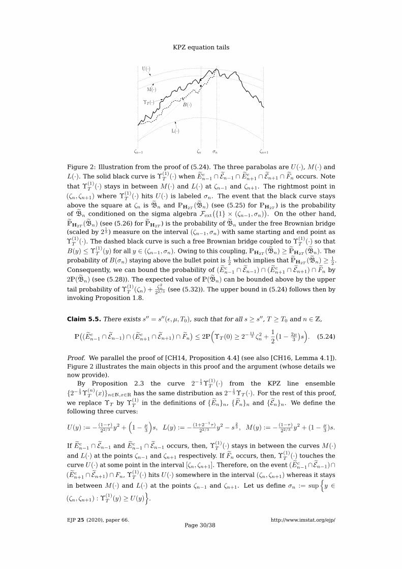
KPZ equation tails

ζn−1 ζn ζn+1σn

M(·)

U(·)

L(·)

ΥT (·) B(·)

Figure 2: Illustration from the proof of (5.24). The three parabolas are U(·), M(·) and

L(·). The solid black curve is Υ(1)T (·) when Ecn−1 ∩ En−1 ∩ Ecn+1 ∩ En+1 ∩ Fn occurs. Note

that Υ(1)T (·) stays in between M(·) and L(·) at ζn−1 and ζn+1. The rightmost point in

(ζn, ζn+1) where Υ(1)T (·) hits U(·) is labeled σn. The event that the black curve stays

above the square at ζn is Bn and PH2T(Bn) (see (5.25) for PH2T

) is the probabilityof Bn conditioned on the sigma algebra Fext

(1 × (ζn−1, σn)

). On the other hand,

PH2T(Bn) (see (5.26) for PH2T

) is the probability of Bn under the free Brownian bridge(scaled by 2

13 ) measure on the interval (ζn−1, σn) with same starting and end point as

Υ(1)T (·). The dashed black curve is such a free Brownian bridge coupled to Υ

(1)T (·) so that

B(y) ≤ Υ(1)T (y) for all y ∈ (ζn−1, σn). Owing to this coupling, PH2T

(Bn) ≥ PH2T(Bn). The

probability of B(σn) staying above the bullet point is 12 which implies that PH2T

(Bn) ≥ 12 .

Consequently, we can bound the probability of (Ecn−1 ∩ En−1) ∩ (Ecn+1 ∩ En+1) ∩ Fn by

2P(Bn) (see (5.28)). The expected value of P(Bn) can be bounded above by the upper

tail probability of Υ(1)T (ζn) +

ζ2n22/3 (see (5.32)). The upper bound in (5.24) follows then by

invoking Proposition 1.8.

Claim 5.5. There exists s′′ = s′′(ε, µ, T0), such that for all s ≥ s′′, T ≥ T0 and n ∈ Z,

P((Ecn−1 ∩ En−1) ∩ (Ecn+1 ∩ En+1) ∩ Fn

)≤ 2P

(ΥT (0) ≥ 2−

113 ζ2

n +1

2

(1− 2µ

3

)s). (5.24)

Proof. We parallel the proof of [CH14, Proposition 4.4] (see also [CH16, Lemma 4.1]).Figure 2 illustrates the main objects in this proof and the argument (whose details wenow provide).

By Proposition 2.3 the curve 2−13 Υ

(1)T (·) from the KPZ line ensemble

2− 13 Υ

(n)T (x)n∈N,x∈R has the same distribution as 2−

13 ΥT (·). For the rest of this proof,

we replace ΥT by Υ(1)T in the definitions of Enn, Fnn and Enn. We define the

following three curves:

U(y) := − (1−τ)22/3 y

2 +(

1− µ3

)s, L(y) := − (1+2−1τ)

22/3 y2 − s 23 , M(y) := − (1−τ)

22/3 y2 + (1− µ

3 )s.

If Ecn−1 ∩ En−1 and Ecn−1 ∩ En−1 occurs, then, Υ(1)T (·) stays in between the curves M(·)

and L(·) at the points ζn−1 and ζn+1 respectively. If Fn occurs, then, Υ(1)T (·) touches the

curve U(·) at some point in the interval [ζn, ζn+1]. Therefore, on the event (Ecn−1∩En−1)∩(Ecn+1 ∩ En+1)∩Fn, Υ

(1)T (·) hits U(·) somewhere in the interval (ζn, ζn+1) whereas it stays

in between M(·) and L(·) at the points ζn−1 and ζn+1. Let us define σn := supy ∈

(ζn, ζn+1) : Υ(1)T (y) ≥ U(y)

.

EJP 25 (2020), paper 66./38




KPZ equation tails

Recall that ζn−1 < ζn < ζn+1. Consider the following crossing event

Bn :=

Υ(1)T (ζn) ≥ σn − ζn

σn − ζn−1L(ζn−1) +

ζn − ζn−1

σn − ζn−1U(σn)

.

We will use the following abbreviation for the probability measures

PH2T:= P

1,1,(ζn−1,σn),2−13 Υ

(1)T (ζn−1),2−

13 Υ

(1)T (σn),+∞,2−

13 Υ

(2)T

H2T, (5.25)

PH2T:= P

1,1,(ζn−1,σn),2−13 Υ

(1)T (ζn−1),2−

13 Υ

(1)T (σn),+∞,−∞

H2T. (5.26)

Since, (ζn−1, σn) is a 1-stopping domain (see Definition 2.1) for the KPZ line ensem-ble, the strong H2T -Brownian Gibbs property (see Lemma 2.5 of [CH16]) applies to showthat

E[1((Ecn−1 ∩ En−1) ∩ (Ecn+1 ∩ En+1) ∩ Fn

)· 1(Bn)|Fext

(1 × (ζn−1, σn)

)](5.27)

=1((Ecn−1 ∩ En−1) ∩ (Ecn+1 ∩ En+1) ∩ Fn

)· PH2T

(Bn).

By Proposition 2.4, there exists a monotone coupling12 between the probability mea-sures PH2T

and PH2T. Using this and the fact that the probability of Bn increases under

pointwise increase of its sample paths, we have PH2T(Bn) ≥ PH2T

(Bn). Since PH2Tis

the law of a Brownian bridge on the interval (ζn−1, σn) with end points 2−13 Υ

(1)T (ζn−1)

and 2−13 Υ

(1)T (σn), the probability that it stays above the line joining the two end points at

a given intermediate point is 12 . Therefore PH2T

(Bn) ≥ 12 . Plugging this into (5.27) and

taking expectation yields

P((Ecn−1 ∩ En−1) ∩ (Ecn+1 ∩ En−1) ∩ Fn

)≤ 2E

[1((Ecn−1 ∩ En−1) ∩ (Ecn+1 ∩ En+1) ∩ Fn) · 1(Bn)

]. (5.28)

Now, we bound the r.h.s. of (5.28). Note the following holds13 for all n ∈ Z:

(σn − ζn)ζ2n−1 + (ζn − ζn−1)σ2

n

σn − ζn−1− ζ2

n = (σn − ζn)(ζn − ζn−1) ≤ 1

s2+2δ, (5.29)

− 12 (σn − ζn)ζ2

n−1 + (ζn − ζn−1)σ2n

σn − ζn−1+

1

2ζ2n = −1

2(σn − ζn)(ζn − ζn−1) +

3

2

ζn − ζn−1

σn − ζn−1σ2n,

(5.30)

3

2

ζn − ζn−1

σn − ζn−1σ2n −

1

2ζ2n ≥

1

4ζ2n − 2

|ζn|s1+δ

≥ 1

8ζ2n −

32

s2+2δ. (5.31)

Combining (5.29), (5.30) and (5.31) yields

σn − ζnσn − ζn−1

L(ζn−1) +ζn − ζn−1

σn − ζn−1U(σn) ≥ − (1− 8−1τ)

22/3ζ2n −

(4 + 34τ)

22/3s2+2δ+

1

2

((1− µ

3

)s− s 2

3

).

This implies that when Bn occurs, Υ(1)T (ζn) will be greater than the r.h.s above. The r.h.s

is bounded below by −2−23 (1− 8−1τ) + 1

2

(1− 2µ

3

)s when s is large enough. Hence, we

have

r.h.s. of (5.28) ≤ 2P(Bn) ≤ 2P

(Υ

(1)T (ζn) ≥ − (1− 8−1τ)

22/3ζ2n +

1

2

(1− 2µ

3

)s

). (5.32)

Now, the claim follows from (5.28) and (5.32) by recalling that Υ(1)T (ζ2

n)+ζ2n

22/3

d= ΥT (0).

12If B is PH2Tdistributed and B is PH2T

distributed, then, under the coupling, B(y) ≥ B(y), ∀y ∈(ζn−1, σn)

13To see the first inequality of (5.31), note that (ζn − ζn−1)/(σn − ζn−1) ≥ 12

and σ2n ≥ ζ2n − 2|ζn|s−(1+δ);

the second inequality follows from 8−1ζ2n − 2|ζn|s−(1+δ) ≥ 0 for all |n| ≥ 16.

EJP 25 (2020), paper 66./38




KPZ equation tails

Using (5.24) and a similar analysis as in Lemma 5.1, there exist s′′ = s′′(ε, µ, T0) andC ′ = C ′(ε, T0) such that for all s ∈ [maxs′′, s0,∞),

∑n∈Z

P((Ecn−1 ∩ En−1) ∩ (Ecn+1 ∩ En+1) ∩ Fn

)≤

C ′e−

√2

3 (1−ε)(1−µ)s3/2 if s ∈ (s1, s2],

C ′e−√

23 ε(1−µ)s3/2 if s ∈ (s1, s2].

where (s1, s2] := [s0,∞)\(s1, s2]. Combining this with (5.23), we arrive at (5.22).

Final step of the proof of Proposition 5.1: Define s′0 := maxs, s′, s′′ where s, s′, s′′ aretaken from Lemmas 5.1, 5.3 and 5.4 respectively.

(1) Owing to (5.21) and (5.22), when T0 > π, there exists Θ = Θ(ε, T0) such that for alls ∈ [maxs′0, s0,∞)

P

(Af ∩

(⋃n∈Z

En

)c)≤

Θe−

√2

3 (1−ε)(1−µ)s3/2 when s ∈ [s0, s1] ∪ (s2,∞),

Θe−√

23 ε(1−µ)s3/2 when s ∈ (s1, s2].

(5.33)

Plugging (5.33) and (5.10) of Lemma 5.1 into the r.h.s. of (5.9) yields (5.3).

(2) When T0 ∈ (0, π), the proof of (5.4) follows in the same way as in the proof of (5.3)

by assuming P(ΥT (0) > s) ≤ e−cs3/2 for all s ≥ s0 and T ∈ [T0, π].


Let I be a subinterval of [−M,M ] with |I| = θ such that f(y) ≥ −κ for all y ∈ I. Assumes is large enough such that s−n+2 ≤ θ. Let χ1 ≤ χ2 ∈ I be such that χ2 − χ1 = s−n+2.Define

Wi :=

ΥT (−χi) ≥ −χ2i

22/3+(1 + 2µ

3

)s

for i = 1, 2,

Wint :=

ΥT (y) ≥ − y2

22/3+(1 + µ

3

)s for all y ∈ (−χ2,−χ1)

.

We claim that there exists s′ = s′(µ, θ, κ, T0) such that for all s ≥ s′ and T ≥ T0

P(W1 ∩W2 ∩Wint) ≤ P(hfT (0) ≥ s). (5.34)

To show this, assume that the eventW1 ∩W2 ∩Wint occurs. Then14,∫ ∞−∞

eT1/3(ΥT (y)+f(−y))dy ≥

∫−I

eT1/3(ΥT (y)+f(−y))dy ≥ 2θeT

1/3((1+µ/3)s−κ) ≥ eT1/3s

where the last inequality holds when s exceeds some s′(µ, θ, κ, T0). This shows that

P(W1 ∩W2 ∩Wint

)≤ P

(∫ ∞−∞

eT1/3(ΥT (y)+f(y))dy ≥ eT

1/3s)

= P(hfT (0) ≥ s).

To finish the proof of (5.5) we combine (5.34) with (5.35) below and take s0 =

maxs′, s′′.Claim 5.6. There exist s′′ = s′′(µ, n, T0), K = K(µ) > 0 such that for all s ≥ s′′ andT ≥ T0,

P (W1 ∩W2 ∩Wint) ≥(P(ΥT (0) >

(1 + 2µ

3

)s))2

− e−Ksn

. (5.35)

14We use below −I as a shorthand notation for x : −x ∈ I

EJP 25 (2020), paper 66./38




KPZ equation tails

Proof. We start by writing P(W1 ∩W2 ∩Wint

)= P(W1 ∩W2)−P(W1 ∩W2 ∩Wc

int). Usingthe FKG inequality from (1.10),

P(W1 ∩W2) ≥ P(W1)P(W2) ≥(P(ΥT (0) >

(1 + 2µ

3

)s))2

(5.36)

where the last inequality follows from Proposition 1.8. Note that (5.36) provides alower bound for the first term on the r.h.s. of (5.35). To complete the proof, we needto demonstrate an upper bound on P(W1 ∩ W2 ∩ Wc

int) of the form e−Ksn

. To achievethis we go to the KPZ line ensemble and use its Brownian Gibbs property. We mayreplace ΥT by Υ

(1)T in all definitions without changing the value of P(W1 ∩W2 ∩Wc

int)

(see Proposition 2.3). Let us define

PH2T:= P

1,1,(−χ2,−χ1),2−13 Υ

(1)T (−χ2),2−

13 Υ

(1)T (−χ1),+∞,2−

13 Υ

(2)T

H2T,

PH2T:= P

1,1,(−χ2,−χ1),2−13 Υ

(1)T (−χ2),2−

13 Υ

(1)T (−χ1),+∞,−∞

H2T.

Using the H2T -Brownian Gibbs property of the KPZ line ensemble 2− 13 Υ

(n)T (x)n∈N,x∈R,

P(W1 ∩W2 ∩Wc

int

)= E

[1(W1 ∩W2) · PH2T

(Wcint)]. (5.37)

Via Proposition 2.4, there exists a monotone coupling between PH2Tand PH2T

sothat

PH2T(Wc

int) ≤ PH2T(Wc

int). (5.38)

Recall that PH2Tis the measure of a Brownian bridge on (−χ2,−χ1) with starting and

end points at 2−13 Υ

(1)T (−χ2) and 2−

13 Υ

(1)T (−χ1). Applying (5.38) into the r.h.s. of (5.37)

implies

1(W1 ∩W2) · PH2T(Wc

int) ≤ P1,1,(−χ2,−χ1),−χ

222 +2−

13

(1+

2µ3

)s,−χ

212 +2−

13

(1+

2µ3

)s

free

(Wc

int

).

Therefore (using Lemma 2.2 for the second inequality) there exists K = K(µ) such that

l.h.s. of (5.37) ≤ P1,1,(−χ2,−χ1),−χ

222 +2−

13

(1+

2µ3

)s,−χ

212 +2−

13

(1+

2µ3

)s

free (Wcint) ≤ e−Ks

n

.


Theorem 1.14 follows by combining all three parts of Theorem 1.11 with the followingresults which are in the same spirit of Proposition 5.1 and 5.2 respectively.

Recall ΥT and hBrT from (1.8) and (1.13) respectively.

Proposition 5.3. Fix ε, µ ∈ (0, 12 ).

(1) Fix T0 > π. Suppose there exists s0 = s0(ε, T0) and for any T ≥ T0, there exists2 = s2(ε, T ) and s3 = s3(ε, T ) with s1 ≤ s2 ≤ s3 such that for any s ∈ [s0,∞),

P(ΥT (0) > s

)≤

e−43 (1−ε)s

32 if s ∈ [s0, s1] ∪ (s2,∞),

e−43 εs

32 if s ∈ (s1, s2].

(5.39)

Then, there exists s′0 = s′0(ε, µ, T0) such that for any T > T0 and s ∈ [maxs′0, s0,∞),we have (recall s0, s1 and s2 from (5.2))

P(hBrT (0) > s

)≤

e−√

23 (1−ε)(1−µ)s3/2 + e

− 19√

3(µs)3/2 if s ∈ [s0, s1] ∪ (s2,∞),

e−√

23 ε(1−µ)s3/2 + e

− 19√

3(µs)3/2 if s ∈ (s1, s2].

(5.40)

EJP 25 (2020), paper 66./38




KPZ equation tails

(2) For any T0 ∈ (0, π), there exists s′0 = s′0(T0) > 0 satisfying the following: if there

exists s0 = s0(T0) > 0 such that P(ΥT (0) > s) ≤ e−cs3/2 for all s ≥ s0 and T ∈ [T0, π],then,

P(hfT (0) > s

)≤ e−cs

3/2

, ∀s ∈ [maxs′0, s0,∞), T ∈ [T0, π]. (5.41)

Proposition 5.4. Fix µ ∈ (0, 12 ), n ∈ Z≥3 and T0 > π. Then, there exist s0 =

s0(µ, n, T0),K = K(µ, n) > 0 such that for all s ≥ s0 and T ≥ T0,

P(hBrT (0) > s) ≥

(P(

ΥT (0) >(1 +

2µ

3

)s))2

− e−Ksn

. (5.42)

We prove these propositions using similar arguments as in Section 5.1.1 and 5.1.2.Propositions 5.3 and 5.4 are proved in Sections 5.2.1 and Section 5.2.2, respectively.

Proof of Theorem 1.14. This theorem is proved in the same way as Theorem 1.4 bycombining Proposition 5.3 and Proposition 5.4. We do not duplicate the details.


To prove this proposition, we use similar arguments as in Section 5.1.2. Let τ ∈ (0, 12 ) be

fixed (later we choose its value). Recall the events En and Fn from Section 5.1.1 anddefine

ABr :=

∫ ∞−∞

eT1/3(

ΥT (y)+B(−y))dy > esT

1/3

where B is a two sided Brownian motion with diffusion coefficient 2

13 and B(0) = 0.

Appealing to Proposition 1.7, we see that P(hBrT (0) > s) = P(ABr). Now, we write

P(ABr

)≤∑n∈Z

P(En)

+ P(ABr ∩

( ⋃n∈Z

En)c ∩ ( ⋃

n∈ZFn))

+ P(ABr ∩

( ⋃n∈Z

En)c ∩ ( ⋃

n∈ZFn)c)

. (5.43)

Using Lemma 5.1 (see (5.10)) and Lemma 5.4 (see (5.22)) we can bound the first twoterms on the right side hand side of (5.43). However, unlike in Theorem 5.1, the lastterm in (5.43) is not zero. We now provide an upper bound to this term.

Claim 5.7. There exists s′ = s′(τ, µ) such that for all s ≥ s′,

P(ABr ∩

( ⋃n∈Z

En)c ∩ ( ⋃

n∈ZFn)c) ≤ exp

(−√

(1−2τ)

3√

6

(2µs3 + log

((2π)−1τ(2T )

13

)) 32

).

(5.44)

Proof. Note thatABr ∩

( ⋃n∈Z

En)c ∩ ( ⋃

n∈ZFn)c ⊆ ∫ ∞

−∞eT 1/3

(− (1−τ)y2

22/3+B(−y)

)dy ≥ e3−1µsT 1/3

.

(5.45)

We claim that

r.h.s. of (5.45) ⊆

maxy∈R

− (1− 2τ)y2 +B(−y)

22/3

≥ 1

3µs+ 12 log((2π)−1τ(2T )

13 ).

(5.46)

EJP 25 (2020), paper 66./38




KPZ equation tails

To see this by contradiction, assume the complement of the r.h.s. of (5.46). This impliesthat ∫ ∞

−∞eT 1/3

(− (1−τ)y2

22/3+B(−y)

)dy <

√(2π)−1τ(2T )1/3e3−1µsT 1/3

∫ ∞−∞

e−τy2T 1/3/2

23 dy

= e3−1µsT 1/3

.

Therefore, (5.46) holds. Applying Proposition 2.3 (with ξ = 12 ), we see that

P(r.h.s. of (5.46)

)≤ 1√

3exp

(−√

(1− 2τ)

3√

6

(2µs

3+ log((2π)−1τ(2T )

13 )) 3

2

).

when s is large enough. Combining this with (5.45), we arrive at (5.44) showing theclaim.

Now, we turn to complete the proof of Proposition 5.3. Choosing τ = 18 , we notice

r.h.s. of (5.44) ≤ exp(− 1

9√

3

(µs− 3 log(16π)

2

)3/2), ∀T > π.

For the rest of this proof, we will fix some T ≥ T0 and assume that there exist s0 =

s0(ε, T0), s1 = s1(ε, T ) and s2 = s2(ε, T ) with s1 ≤ s2 such that (5.39) is satisfied forall s ∈ [s0,∞). Owing to (5.10) of Lemma 5.1 and (5.22) of Lemma 5.4, there existΘ = Θ(ε, T0) and s = s(ε, µ, T0) such that for all s ∈ [maxs, s0),∞),

P( ⋃n∈Z

En

)+ P

(ABr ∩

( ⋃n∈Z

En)c ∩ ( ⋃

n∈ZFn))≤

Θe−

√2

3 (1−ε)(1−µ)s3/2 if s ∈ (s1, s2],

Θe−√

23 ε(1−µ)s3/2 if s ∈ (s1, s2]

where (s1, s2] = [s0,∞)\(s1, s2]. Combining this with (5.44) and plugging into (5.43), weget (5.40) for all T > T0 ≥ π. In the case when T0 ∈ (0, π), we obtain (5.41) in a similarway as in the proof of (5.4) of Proposition 5.1 by combining the inequality of the abovedisplay with P(ΥT (0)) ≤ e−cs3/2 for all s ≥ s0 and T ∈ [T0, π].


We use similar argument as in Proposition 5.2. The main difference from the proof ofProposition 5.2 is that we do not expect (5.34) to hold because the initial data is now atwo sided Brownian motion, hence, (1.3) of Definition 1.1 is not satisfied. However, itholds with high probability which follows from the following simple consequence of thereflection principle for B (a two-sided Brownian motion with diffusion coefficient 2

13 and

B(0) = 0)

P(Ms

)≤ e−

µ2

36 sn

, where Ms =

miny∈[−s−n+2,s−n+2]

B(t) ≤ −µ6 s. (5.47)

To complete the proof, let us define:

W± :=

ΥT (±s−n+2) ≥ − 1

22/3s2(n−2)+(1 + 2µ

3

),

Wint :=

ΥT (y) ≥ − y2

22/3+(1 + µ

3

)s, ∀y ∈ [−s−n+2, s−n+2]

.

We claim that there exists s′ = s′(µ, n, T0) such that for all s ≥ s′ and T ≥ T0,

P(hBrT (0) > s

)≥ P

(W+ ∩ W− ∩ Wint

)− e−

µ2

36 sn

. (5.48)

EJP 25 (2020), paper 66./38




KPZ equation tails

To see this, assume W+ ∩ W− ∩ Wint ∩Ms occurs. Then, for s large enough,∫ ∞−∞

eT1/3(

ΥT (y)+B(−y))dy ≥

∫ s−n+2

−s−n+2

eT 1/3

(− 1

22/3s2(n−2)+(1+µ

6 )s)dy > esT

1/3

. (5.49)

By Proposition 1.7, the event l.h.s. of (5.49) ≥ r.h.s. of (5.49) equals hBrT (0) > s.

Therefore (using (5.47) for the second inequality) we arrive at the claimed (5.48) via

P(hBr

T (0) > s)≥ P

(W+ ∩ W− ∩ Wint ∩Ms

)≥ P

(W+ ∩ W− ∩ Wint

)− e−

µ2

36 sn

.

To finish the proof of Proposition 5.4 we use a similar argument as used to prove(5.35). For any n ∈ Z≥3, there exists s′′ = s′′(µ, n, T0) such that for all s ≥ s′′ and T ≥ T0,

P(W+ ∩ W− ∩ Wint

)≥(P(ΥT (0) >

(1 + 2µ

3

)s))2

− e−Ksn

.

Combining this with (5.48) and taking s0 = maxs′, s′′, we arrive at (5.42) for all s ≥ s0.

References

[ACQ11] G. Amir, I. Corwin, and J. Quastel. Probability distribution of the free energy of thecontinuum directed random polymer in 1 + 1 dimensions. Comm. Pure Appl. Math.,64(4):466–537, 2011. MR-2796514

[AGZ10] G. W. Anderson, A. Guionnet, and O. Zeitouni. An introduction to random matrices,volume 118 of Cambridge Studies in Advanced Mathematics. 2010. MR-2760897

[Apo76] T. M. Apostol. Introduction to analytic number theory. Springer-Verlag, 1976. MR-0434929

[BFP10] J. Baik, P. L. Ferrari, and S. Péché. Limit process of stationary TASEP near thecharacteristic line. Comm. Pure Appl. Math., 63(8):1017–1070, 2010. MR-2642384

[BR00] J. Baik and E. M. Rains. Limiting distributions for a polynuclear growth model withexternal sources. J. Statist. Phys., 100(3-4):523–541, 2000. MR-1788477

[BC17] G. Barraquand and I. Corwin. Random-walk in beta-distributed random environment.Probab. Theory Related Fields, 167(3-4):1057–1116, 2017. MR-3627433

[BC95] L. Bertini and N. Cancrini. The stochastic heat equation: Feynman-Kac formula andintermittence. J. Stat. Phys., 78(5-6):1377–1401, 1995. MR-1316109

[BC14] A. Borodin and I. Corwin. Macdonald processes. In XVIIth International Congresson Mathematical Physics, pages 292–316. World Sci. Publ., Hackensack, NJ, 2014.MR-3204480

[BCFV15] A. Borodin, I. Corwin, P. Ferrari, and B. Veto. Height fluctuations for the stationaryKPZ equation. Math. Phys. Anal. Geom., 18(1):Art. 20, 95, 2015. MR-3366125

[BG16] A. Borodin and V. Gorin. Moments match between the KPZ equation and the Airypoint process. SIGMA, 12:Paper No. 102, 7, 2016. MR-3564786

[CD15] L. Chen and R. C. Dalang. Moments and growth indices for the nonlinear stochasticheat equation with rough initial conditions. Ann. Probab., 43(6):3006–3051, 2015.MR-3433576

[CHN16] L. Chen, Y. Hu, and D. Nualart. Regularity and strict positivity of densities for thenonlinear stochastic heat equation. Memoirs of American Mathematical Society,2016.

[Com17] F. Comets. Directed polymers in random environments, volume 2175 of LectureNotes in Mathematics. Springer, Cham, 2017. MR-3444835

[CJK13] D. Conus, M. Joseph, and D. Khoshnevisan. On the chaotic character of the stochasticheat equation, before the onset of intermitttency. Ann. Probab., 41(3B):2225–2260,2013. MR-3098071

EJP 25 (2020), paper 66./38


http://www.ams.org/mathscinet-getitem?mr=2796514
















KPZ equation tails

[Cor12] I. Corwin. The Kardar-Parisi-Zhang equation and universality class. Random Matri-ces Theory Appl., 1(1):1130001, 76, 2012. MR-2930377

[CG] I. Corwin and P. Ghosal. Lower tail of the KPZ equation. Duke Math. J., 169(7):1329–1395, 2020. MR-4094738

[CGK+18] I. Corwin, P. Ghosal, A. Krajenbrink, P. Le Doussal, and L.-C. Tsai. Coulomb-gaselectrostatics controls large fluctuations of the KPZ equation. Phys. Rev. Lett., Aug2018. MR-4094738

[CH14] I. Corwin and A. Hammond. Brownian Gibbs property for Airy line ensembles. Invent.Math., 195(2):441–508, 2014. MR-3152753

[CH16] I. Corwin and A. Hammond. KPZ line ensemble. Probab. Theory Related Fields,166(1-2):67–185, 2016. MR-3547737

[CQ13] I. Corwin and J. Quastel. Crossover distributions at the edge of the rarefaction fan.Ann. Probab., 41(3A):1243–1314, 2013. MR-3098678

[FS006] P. L. Ferrari, H. Spohn. Scaling limit for the space-time covariance of the stationarytotally asymmetric simple exclusion process. Comm. Math. Phys., 265(1):45–46,2006. MR-2217296

[GKM07] J. Gärtner, W. König, and S. Molchanov. Geometric characterization of intermittencyin the parabolic Anderson model. Ann. Probab., 35(2):439–499, 2007. MR-2308585

[GM90] J. Gärtner and S. A. Molchanov. Parabolic problems for the Anderson model. I.Intermittency and related topics. Comm. Math. Phys., 132(3):613–655, 1990. MR-1069840

[GS13] N. Georgiou and T. Seppäläinen. Large deviation rate functions for the partitionfunction in a log-gamma distributed random potential. Ann. Probab., 41(6):4248–4286, 2013. MR-3161474

[Gho] P. Ghosal. Moments of the SHE under delta initial measure. arXiv:1808.04353.

[GT11] P. Groeneboom and N. M. Temme. The tail of the maximum of Brownian motionminus a parabola. Electron. Commun. Probab., 16:458–466, 2011. MR-2831084

[Hai13] M. Hairer. Solving the KPZ equation. Ann. of Math. (2), 178(2):559–664, 2013.MR-3071506

[HLDM+18] A. K. Hartmann, P. Le Doussal, S. N. Majumdar, A. Rosso, and G. Schehr. Highprecision simulation of the height distribution for the kpz equation. Europhys. Lett.,121:67004, 2018.

[IS04] T. Imamura and T. Sasamoto. Fluctuations of the one-dimensional polynuclear growthmodel with external sources. Nuclear Phys. B, 699(3):503–544, 2004. MR-2098552

[Jan15] Chris Janjigian. Large deviations of the free energy in the o’connell-yor polymer. J.Statis. Phys., 160:1054–1080, 2015. MR-3373651

[JYC09] M. Jeanblanc, M. Yor, and M. Chesney. Mathematical methods for financial markets.Springer Finance. Springer-Verlag London, Ltd., London, 2009. MR-2568861

[KMS16] A. Kamenev, B. Meerson, and P. V. Sasorov. Short-time height distribution in theone-dimensional kardar-parisi-zhang equation: Starting from a parabola. Phys. Rev.E, 94:032108, 2016. MR-3731817

[KS91] I. Karatzas and S. E. Shreve. Brownian motion and stochastic calculus. 1991. MR-1121940

[Kho14] D. Khoshnevisan. Analysis of stochastic partial differential equations, volume 119 ofCBMS Regional Conference Series in Mathematics. AMS, 2014. MR-3222416

[KKX17] D. Khoshnevisan, K. Kim, and Y. Xiao. Intermittency and multifractality: a case studyvia parabolic stochastic PDEs. Ann. Probab., 45(6A):3697–3751, 2017. MR-3729613

[Kno70] M. I. Knopp. Modular functions in analytic number theory. Mark. Pub. Co., 1970.MR-0265287

[KL18a] A. Krajenbrink and P. Le Doussal. Large fluctuations of the KPZ equation in ahalf-space. SciPost Phys. 5, 2018.

EJP 25 (2020), paper 66./38



























KPZ equation tails

[KL18b] A. Krajenbrink and P. Le Doussal. Simple derivation of the (−λH)5/2 tail for the 1DKPZ equation. J. Stat. Mech., 2018. MR-3832292

[LDMS16] P. Le Doussal, S. N. Majumdar, and G. Schehr. Large deviations for the height in 1dkardar-parisi-zhang growth at late times. EPL, 113(6):60004, 2016.

[Mol] S. Molchanov. Reaction-diffusion equations in the random media: localization andintermittency. In Nonlinear stochastic PDEs (Minneapolis, MN, 1994). MR-1395894

[MF14] G. R. Moreno Flores. On the (strict) positivity of solutions of the stochastic heatequation. Ann. Probab., 42(4):1635–1643, 2014. MR-3262487

[Mue91] C. Mueller. On the support of solutions to the heat equation with noise. Stoch. &Stoch. Rep., 37(4):225–245, 1991. MR-1149348

[MN08] C. Mueller and D. Nualart. Regularity of the density for the stochastic heat equation.Electron. J. Probab., 13:no. 74, 2248–2258, 2008. MR-2469610

[PS04] Michael Prähofer and Herbert Spohn. Exact scaling functions for one-dimensionalstationary KPZ growth. J. Statist. Phys., 115(1-2):255–279, 2004. MR-2070096

[Qua12] J. Quastel. Introduction to KPZ. In Current developments in mathematics, 2011,pages 125–194. Int. Press, Somerville, MA, 2012. MR-3098078

[RRV11] J. A. Ramírez, B. Rider, and B. Virág. Beta ensembles, stochastic Airy spectrum, anda diffusion. J. Amer. Math. Soc., 24(4):919–944, 2011. MR-2813333

[SMP17] P. Sasorov, B. Meerson, and S. Prolhac. Large deviations of surface height in the1 + 1-dimensional Kardar-Parisi-Zhang equation: exact long-time results for λH<0.Journal of Statistical Mechanics: Theory and Experiment, 2017. MR-3673439

[Tsa] L.-C. Tsai. Exact lower tail large deviations of the KPZ equation. arXiv:1809.03410.

Acknowledgments. We thank J. Baik, G. Barraquand, S. Das, P. Le Doussal, A. Kra-jenbrink, J. Quastel, L.-C. Tsai, and B. Virag for helpful conversations and comments,as well as an anonymous referee for many helpful comments. I.C. was supported inpart by a Packard Fellowship for Science and Engineering, and by NSF DMS-1811143,DMS-1664650.

EJP 25 (2020), paper 66./38














KPZ equation tails for general initial data

Documents

Transcript of KPZ equation tails for general initial data