KPI Assessment Methodology Lead Beneficiary: ICCS/NTUA

THEME [ENERGY.2012.7.1.1] Integration of Variable Distributed Resources in Distribution Networks

(Deliverable –2.4)

KPI Assessment Methodology

Lead Beneficiary:

ICCS/NTUA

December 2013

December

Deliverable – D 2.4: KPI assessment methodology

2/27

Table of Contents

1. EXECUTIVE SUMMARY ............................................................................................ 6

2. INTRODUCTION....................................................................................................... 7

3. SUSTAINABLE PROJECT - KPIS OVERVIEW ................................................................ 9

3.1 Level 1 KPIs Assessment....................................................................................... 9

3.2 Level 2 KPIs Assessment....................................................................................... 9

3.3 Level 3 KPIs Assessment......................................................................................12

3.4 Level 4 KPIs Assessment......................................................................................12

4. SUSTAINABLE FUNCTIONALITIES IMPACT ON PROJECT KPIS ...................................13

5. DEFINITION OF SUSTAINABLE KPIS .........................................................................15

5.1. Deferred Transmission and Distribution Capacity Investment ..............................15

5.2. Reduction of Technical Losses .............................................................................16

5.3. Allowable maximum DG power without branch overload and voltage limit violations (Increase of RES Hosting Capacity) .......................................................16

5.4. Share of Electrical Energy produced by RES .........................................................17

5.5. Voltage and Power Quality Performance .............................................................18

5.6. Reduction of Carbon Emissions ...........................................................................19

5.7. Reduction in RES cut-off due to congestion .........................................................19

5.8. Optimized use of Assets......................................................................................20

5.9. Forecast Improvement (Level 4 KPI) ....................................................................22

5.10. State Estimation quality Indices (Level 4 KPI) ....................................................24

6. REFERENCES ...........................................................................................................27


3/27

List of Figures

Figure 1. EEGI KPI developed framework for impact KPIs

Figure 2. Impact of Sustainable functionalities on project KPIs


4/27

List of Acronyms and Abbreviations

CHP Combined Heat and Power

CL Controllable Load

DG Distributed Generation

DoW Description of Work

DSM Demand Side Management

DSO Distribution System Operator

DTC Distribution Transformer Controller

Energy Box Smart Meter

EV Electric Vehicle

IED Intell igent Electronic Device

HV High Voltage

KPI Key Performance Indicator

LV Low Voltage

MV Medium Voltage

NWP Numerical Weather Predictions

OLTC On-Load Tap Changing

OPF Optimal Power Flow

RES Renewable Energy Sources

RTU Remote Terminal Unit

SCADA/DMS Supervisory Control and Data Acquisition / Distribution Management System

SSC Smart Substation Controller

STOR Storage Device

TSO Transmission System Operator

TVPP Technical Virtual Power Plant

uG Microgeneration

VHV Very High Voltage

VPP Virtual Power Plant


5/27

Authors

Authors Organization E-mail

Nikos Hatziargyriou ICCS/NTUA [email protected]

Stavros Papathanassiou ICCS/NTUA [email protected]

George Korres ICCS/NTUA [email protected]

Pavlos Georgilakis ICCS/NTUA [email protected]

Aris Dimeas ICCS/NTUA [email protected]

Despina Koukoula ICCS/NTUA [email protected]

Kai Struntz TUB [email protected]

João A. Peças Lopes INESCP [email protected]

Luis González Sotres UPC [email protected]

Sami Abdelrahman UNIMAN [email protected]

Pedro Godinho Matos EDPD [email protected]

Diogo Lopes EDPD [email protected]

António Aires Messias EDPD [email protected]

Access: Project Consortium

European Commission

Public X

Status: Draft version

Submission for Approval

Final Version X

mailto:[email protected]














6/27

1. Executive Summary

This deliverable provides the KPIs and the KPIs’ assessment methodology for the pilot

installations and the proof of concept demonstration networks of the SuSTAINABLE

project. Starting with the KPIs defined within the EEGI framework (Level 1 and Level 2

KPIs), the document focuses on the Level 3 KPIs that will be used to evaluate

quantitatively the benefits of the methods and functionalities developed within

Sustainable and applied on the actual pilot and demonstration networks.

The Level 3 KPIs are adopted from the DoW and are optimized, as follows:

1) Deferred Transmission and Distribution Capacity Investment;

2) Reduction of Technical Losses

3) Allowable maximum DG power without branch overload and voltage limit violations;

4) Share of electrical energy produced by Renewable sources;

5) Voltage and Power Quality performance indices;

6) Reduction of Carbon Emissions;

7) Reduction in RES cut-off due to congestion;

8) Optimized use of Assets

A detailed definition and calculation formulas are also provided in the present document.

Finally, a number of indices to evaluate the accuracy and quality of the developed

algorithms is provided as a Level 4 KPIs.


7/27

2. Introduction

Description of the Task 2.4 “Definition of use case requirements and proof-of-concept scenarios characterization” from the Description of Work (DoW):

This task will prepare the proof-of-concept and validation activities by specifying the requirements in terms of distribution network models, parameters, and scenarios and

identifying a HV/MV substation and one or more MV/LV substations, with significant amounts of DG, where the demo will be run. It will detail actual regulatory schemes in study cases. Finally, the proof-of-concept and validation KPIs will be identified, namely

the ones referred in the following table. Call Requirements: KPI

• Technically and economically viable deployment of smart grids solutions: 1) Deferred Transmission and Distribution Capacity Investment; 2) Reduction of Technical Losses

• Integrating a large share of distributed renewable generation units in distribution networks, Substantial increase of the hosting capacity for medium- and small-size

renewable sources (mainly wind and PV farms) in existing medium- and low-voltage networks, Allow distribution networks to be operated with reverse flows of electricity at times of high renewable electricity generation and low load:

3) Allowable maximum DG power without branch overload and overvoltage risks; 4) Share of electrical energy produced by Renewable sources;

5) Voltage and Power Quality performance indices; 6) Reduction of Carbon Emissions; 7) Reduction in RES cut-off due to congestion;

8) Ratio of Renewable Generation and Load • Effective planning of necessary network reinforcements, Better observability of distributed resources:

9) Percentage of nodes with DG monitored in real time; 10) Allowable maximum injection of DG without congestion risk; 11) Optimized use of Assets

This task will establish the scenarios to be implemented in WP5 and WP6 where the

current conditions of pilot sites will be complemented with the tools developed along the SuSTAINABLE project. Two main validation sites will be used with high potential for extracting objective conclusions regarding our proposed objective – the InovGrid in Portugal and Rhodes Island in Greece. Also, for more complex functionalities, proof -of-

concept demonstrations (simulations) will be held at pilot sites in Germany, UK, Greece (Meltemi) and the Laboratory facilities of INESCP, ICCS and the SENSE lab at TUB.


8/27

This document includes the KPI assessment methodology for the tools of SuSTAINABLE

project. For the KPIs the EEGI framework is adopted as described in the following figure.

Figure 2 EEGI KPI developed framework for impact KPIs

As adopted from [1] KPIs are distinguished in three levels:

The Level 1 “Overarching KPIs” consists of a limited set of network

performance indicators which trace clear progress brought by EEGI activities

towards its overarching goal;

The Level 2 “Specific KPIs” are indicators defined at Cluster level to quantify

the expected impacts of a group of R&I activities in view of meeting the R&I

roadmap overarching goal;

The Level 3 “Project KPIs” are proposed by each R&I project in view of

detailing further the contribution of each R&I project to level 2 KPIs

Chapter 2 of this document contains the list of KPIs as de fined in Grid+ and the Sustainable project.

Chapter 3 provides the list of relevant Level 3 KPIs for each of the Sustainable functionalities.

Chapter 4 provides a description of the KPIs and the formulas for their calculations.


9/27

3. SuSTAINABLE Project - KPIs Overview

3.1 Level 1 KPIs Assessment

In the Grid+ project, two main KPIs define a global level of assessment. These KPI are:

A.1 Increased network capacity

Increased Network Capacity [NC] is the amount of electrical power that can be transmitted or distributed in the selected frame, for example, to connect new RES generation, to enhance an interconnection, to solve congestion, or even all the transmission capacity of a TSO. In other words, it concerns the possibility to increase the

usage of a given electrical network in order to accept higher levels of integration of distributed generation and consumption, using also available distributed storage units, by exploiting dynamic monitoring and exploiting flexibility in terms of injected power into the grid from generation units and also responsiveness from active loads.

A.2 Increased system flexibility

Increased System Flexibility (SF) is the amount of electrical power (generation or load) that can be modulated to the needs of the system operation within a specific unit of time.

It results from higher levels of controllability of distributed energy resources (generation, load and storage) that allow the management of these resources either locally or in a coordinated manner to enhance the capabilities and efficiency of operation of given electrical network.

The calculation methods for the Level 1 KPIs are described in Annex A of [1] and will be adopted by SUSTAINABLE.


A second level of six, more detailed KPIs was defined in Grid+ in order to further monitor the increasing network capacity and/or system flexibility. The following table , copied

from [1], lists these impact KPIs and their links with the R&I clusters and the three pillars of EU energy policy.


10/27

KPI describing the Expected network capacity & flexibility increases

Related R&I cluster(s)

Compliance with EU policy goals TSO/DSO

Sustainability

Market competit

iveness

Security of

Supply

TSO DSO

B.1 Increased RES & DER hosting capacity

Power Technologies

Integration of DER &

new uses

Network operation

Market Designs

X X X X X

B.2 Reduced energy curtailment of RES and DER Grid Architecture

Network Planning

Power Technologies

Integration of Smart

Customers


new uses

Network Operation

Market Designs

X X X X X

B.3 Power Quality and Quality of Supply X X X X X

B.5 Increased flexibility from energy players X X X X

B.4 Extended asset life time Asset Management X X X

B.6 Improved competitiveness of the electricity market

Integration of Smart

Customers


new uses

Network Operation

Market Designs

X X X

B.7 Increased hosting capacity for Electric Vehicles and other new loads

Network Planning

Integration of DER & new uses

Network Operations

X X X X

The five R&I clusters for DSO are identified as follows:

C1. Integration of smart customers

D1. Active demand for increased flexibility

D2. Energy Efficiency from integration with Smart Homes

C2. Integration of DER and new users


11/27

D3. DSO Integration of small DER

D4. System Integration of medium DER

D5. Integration of Storage in Network Management

D6. Infrastructure to host EV/PHEV

C3. Network Operations

D7. Monitoring and Control of MV Network

D8. Automation and Control of MV Network

D9. Network Management Tools

D10. Smart Metering Data Processing

C4. Network Planning and asset management

D11. New Planning Approaches for Distribution Networks

D12. Asset Management

C5. Market Design

D13. New Approaches for Market Design Analysis

The following table relates the R&I clusters with the KPIs describing the Expected network capacity & flexibility increases.

KPI describing the expected network capacity & flexibility increases

Related R&I cluster(s)

B1. Increased RES & DER hosting capacity

C2. Integration of DER & new users (D3)

C3. Network operation (D8, D9)

C5. Market Design

B2. Reduced energy curtailment of RES and DER

C1.Integration of Smart Customers (D1)

C2. Integration of DER & new users (D3)

C3. Network Operation (D7, D8, D9, D10)

C4. Network Planning (D11)

C5. Market Design

B3. Power Quality and Quality of Supply

B5. Increased flexibility from energy players


12/27


In order to identify in a quantified manner the benefits that can be obtained from the

adoption of the Sustainable functionalities, a more focused and detailed set of KPIs is defined, leading to the third level. These KPIs are the following:

1) Deferred Transmission and Distribution Capacity Investment;

2) Reduction of Technical Losses

3) Allowable maximum DG power without branch overload and voltage limit violations;

4) Share of electrical energy produced by Renewable sources;

5) Voltage and Power Quality performance ;

6) Reduction of Carbon Emissions;

7) Reduction in RES cut-off due to congestion;

8) Optimized use of Assets


Some of the functionalities, like state estimation and forecasting, are enabling functionalities providing the background of the rest of the functionalities and having an

overall clear, but indirect impact on the main KPIs. It is important to evaluate the performance of these functionalities, therefore specific quality indices are suggested for this purpose. These indices, termed Level 4 KPIs, are the following:

9) Forecasting Accuracy

10) State Estimation Quality


13/27

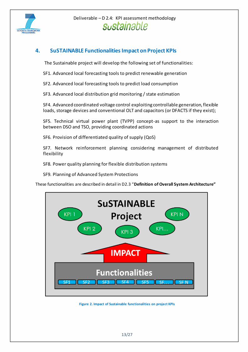
4. SuSTAINABLE Functionalities Impact on Project KPIs

The Sustainable project will develop the following set of functionalities:

SF1. Advanced local forecasting tools to predict renewable generation

SF2. Advanced local forecasting tools to predict load consumption

SF3. Advanced local distribution grid monitoring / state estimation

SF4. Advanced coordinated voltage control exploiting controllable generation, flexible loads, storage devices and conventional OLT and capacitors (or DFACTS if they exist);

SF5. Technical virtual power plant (TVPP) concept-as support to the interaction between DSO and TSO, providing coordinated actions

SF6. Provision of differentiated quality of supply (QoS)

SF7. Network reinforcement planning considering management of distributed flexibility

SF8. Power quality planning for flexible distribution systems

SF9. Planning of Advanced System Protections

These functionalities are described in detail in D2.3 “Definition of Overall System Architecture”

Figure 2. Impact of Sustainable functionalities on project KPIs


14/27

The following Table relates the KPIs identified with the functionalities under development in the Sustainable project.

Sustainable Functionalities impact on project KPIs

KPI1.

Deferred

T&D

Capacity Investment

KPI2.

Reduction

of Technical

Losses

KPI3.

DER

Hosting

KPI4.

Share of

RES

KPI5.

Power

Quality

KPI6.

Reduction

of Carbon

Emissions

KPI7.

Reduction in

DER cut-off

due to congestion

KPI8.

Optimized

use of

Assets

SF1. RES

Forecasting (X) (X) (X) (X) (X) (X)

SF2. Load Forecasting

(X) (X) (X) (X) (X) (X)

SF3.

Monitoring/

State Estimation

(X) (X) (X) (X)

SF4.

Coordinated

Voltage

Control

X X X X X X

SF5. TVPP as

support to

DSO/TSO

X X X X X

SF6. Provision of

Differentiate

d QoS

X X

SF7.

Flexibility based

Reinforceme

nt Planning

X X X X X

SF8. Power Quality

Planning

X X X

SF9.

Advanced Protections

Planning

X X X

(x) Enabling functionalities having indirect impact on KPIs

NOTE: The set of Level 3 KPIs proposed in this deliverable and their corresponding links to the developed functionalities are defined according to the current project state of development and expected outcomes, they might be however modified throughout the project.


15/27

5. Definition of Sustainable KPIs

5.1. Deferred Transmission and Distribution Capacity Investment

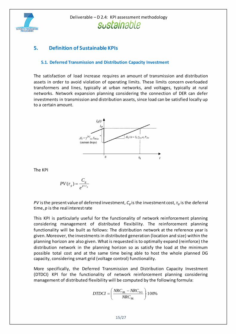
The satisfaction of load increase requires an amount of transmission and distribution

assets in order to avoid violation of operating limits. These limits concern overloaded transformers and lines, typically at urban networks, and voltages, typically at rural networks. Network expansion planning considering the connection of DER can defer

investments in transmission and distribution assets, since load can be satisfied locally up to a certain amount.

The KPI

PV is the present value of deferred investment, Cg is the investment cost, τg is the deferral time, p is the real interest rate

This KPI is particularly useful for the functionality of network reinforcement planning considering management of distributed flexibility. The reinforcement planning

functionality will be built as follows: The distribution network at the reference year is given. Moreover, the investments in distributed generation (location and size) within the planning horizon are also given. What is requested is to optimally expand (reinforce) the

distribution network in the planning horizon so as satisfy the load at the minimum possible total cost and at the same time being able to host the whole planned DG capacity, considering smart grid (voltage control) functionality.

More specifically, the Deferred Transmission and Distribution Capacity Investment (DTDCI) KPI for the functionality of network reinforcement planning considering management of distributed flexibility will be computed by the following formula:

%100

BL

SGBL

NRC

NRCNRCDTDCI

gp

g

ge

CPV

)(


16/27

where:

BLNRC is the net present value of the network reinforcement cost for the baseline

scenario, i.e., 1) without installation of DG in the planning horizon, and 2) without smart grid (DG voltage control) functionality. The BLNRC will be computed by the multi-

objective network reinforcement planning functionality considering no installation of DG in the planning horizon.

SGNRC is the net present value of the network reinforcement cost for the smart grid

case, i.e., 1) considering the installation of the whole scheduled DG in the planning horizon, and, 2) considering the smart grid functioning of the DG (DG voltage control). The SGNRC will be computed by the multi-objective network reinforcement planning

functionality considering installation of DG in the planning horizon in combination with smart grid (DG voltage control) functionality.

5.2. Reduction of Technical Losses

The integration of a greater share of renewable energy resources in distribution grids can potentially reduce losses due to local balancing of energy production and consumption

and thus reduction in power flows. In some cases however, the inversion of power flows related to increased energy production in low load periods increases energy losses.

The KPI calculation will take into account a set of scenarios and boundary conditions to evaluate the percentage of energy losses related to bi -directional power flows

%100

BL

SGBL

L

LLL

LBL is the amount Energy losses (kWh) in baseline scenario evaluated in a defined period.

LSG is the amount of Energy losses (kWh) in smart-grid situation (using network reconfiguration, new devices, ...) evaluated in a defined period.

KPI expressed in % (or kWh if multiplied by LBL)

5.3. Allowable maximum DG power without branch overload and voltage limit

violations (Increase of RES Hosting Capacity)

The need for a large share of RES in energy production leads to conventional reinforcements to enable grid to host them without loss of power quality and reliability.


17/27

The advanced function of RES Hosting Capacity Estimation uses the operational states of the grid including the DER control possibilities and determines the safe upper limit of hosting capacity, without need of new investments.

The parametric RES hosting capacity study provides DSO with information about the total hours during the year, at which the PV installations should accept curtailment orders, to

avoid overvoltage and overcome other operational limitations caused by the grid. This results to an increased RES capacity installation accompanied by minor PV production rejections during critical hours.

Increased network hosting capacity of DG on MV distribution network

%100%

BL

BLSG

HC

HCHCHC

HCBL is the initial (baseline) Hosting Capacity under the primary substation.

HCSG is the Hosting Capacity under the primary substation implementing DER control solutions.

KPI expressed in % (or MW when the KPI is multiplied by HCBL)

5.4. Share of Electrical Energy produced by RES

The KPI calculation will take into account a set of scenarios and boundary conditions to evaluate the percentage of energy production by RES

BLSG

λSG is the share of RES energy in smart-grid situation evaluated in a defined period.

λBL is the share of RES energy in the baseline scenario over the same period.

RES energy shares (%) are calculated as:

LOAD

RES

E

E100

where ERES is the energy generated by RES stations in the defined period and ELOAD is the total load demand in the same period.

KPI expressed in %.


18/27

5.5. Voltage and Power Quality Performance

One of the most essential power quality issues is voltage at the user connection points.

The DNO has the statutory obligation to maintain voltage at all network nodes within a permitted voltage variation band, as stipulated by applicable standards. At the same time, DNOs will always seek to minimize voltage deviation from nominal, to the degree possible.

The increased voltage deviations, especially at remote and weak nodes of the distribution

network, due to large DG penetration is mitigated by optimized exploitation of available regulation means in the network, DER reactive power control, DER active power curtailments and possibly via the incorporation and optimal control of energy storage and demand flexibility.

To quantify the voltage regulation across the entire network, the RMS deviation of the voltage at all nodes is evaluated over the examined time interval:

√∑ (∑ ( )

)

where:

dV is the voltage deviation index for the entire network and time period N is the number of nodes in the network

T is the evaluation period Vi,t is the voltage of node i at time interval t Vn is the nominal voltage

To assess the impact on steady state voltage regulation of advanced network control practices, the following KPI is applied:

%100)(

)()((%)

BCV

BCVSGVV

ud

ududd

where:

dV(uBL) is the voltage deviation index for the base case scenario (standard practice, e.g. typical OLTC action, unity DG power factor, no curtailments, no storage etc.).

dV(uSG) is the voltage deviation index with Smart Grid solutions applied.

For both scenarios, the same network topology, load and DER deployment is assumed.


19/27

5.6. Reduction of Carbon Emissions

This KPI is entirely dependent on KPI 4.4, since the generated RES energy substitutes

practically equal amounts of conventional energy (ignoring the secondary effect of factors such as the change in transmission and distribution losses, the variations in the efficiency and carbon emission factors of generating units providing regulation reserves etc.). If the conventional generation mix is given and the associated average carbon emission factor is

assumed to remain the same, regardless of the achieved RES penetration in the examined network, then the reduction of carbon emissions (CE) KPI is given by:

BLBL

SGBL

CE

CECECE

1

1%100

where CEBL and CESG are the carbon emissions at the two scenarios (base l ine and smart

grid) used to evaluate KPI 4.4, λBL the RES energy share at the base line case and Δλ the KPI 4.4.

5.7. Reduction in RES cut-off due to congestion

Curtailments of DER active power is a last-resort solution that the DNO may apply to deal

with violations of voltage or thermal limits and thus increase DER hosting capacity, because it may raise regulatory, financial and environmental issues. Nevertheless, when such a policy is applied, the amount of energy curtailments can serve as a KPI for the evaluation of the effectiveness of the adopted control practices.

As with the others KPIs, a comparison needs to be made of the curtailed RES energy between a baseline scenario, where basic control and regulation is applied to the network, and one where Smart Grid solutions are being adopted. Nevertheless, it should be pointed out that the application of DER active power control in the baseline scenario already implies the possibility of smart monitoring and control.

Hence, in the first scenario a pseudo “business as usual” scenario will be adopted, where active power curtailments for DER will be applied as the main control variable, while standard voltage control and reactive power regulation will be available. Fitting a large amount of DER in the network will inevitably involve substantial DER energy curtailments.

The smart grid scenario, on the other hand, will comprise the full control possibilities for voltage and reactive power means. This way, it is expected that the same DER capacity will be accommodated in the network with reduced active power cut offs. In both scenarios, all network elements, including loads and installed DG, are exactly the same.

The KPI will be given by the following formula:


20/27

%100

BL

SGBL

E

EEE

where

EBL is the amount of RES energy curtailed in baseline scenario in a def ined period

ESG is the amount of RES energy curtailed in the smart grid scenario over the same period.

5.8. Optimized use of Assets

The variation of the utilization factor of network assets e.g. transformer or feeder capacity is traditionally an important index quantifying the optimal exploitation of

investment in network equipment. Increasing levels of DER penetration will in general lead to a reduction of short term utilization indices, as more power will be generated locally, instead of being transported over the network. On the long run, on the other

hand, this may permit deferral of investments in new T&D capacity, as quantified on KPI 4.1, depending on the load demand and DG generation patterns.

In principle, utilization of assets will mainly depend on installed DG type and capacity, the former because different DER will be characterized by different generation patterns and capacity factors. Coordinated voltage control policies will have a marginal effect on this factor. Hence, this KPI is not deemed suitable to quantify the effect of such policies.

In any case, if this KPI needs to be assessed, the utilization factor of central network

assets can be calculated in two scenarios (baseline–BL and smart grid-SG) using the following formula, e.g. for the HV/MV transformer feeding the MV network under study:

⁄

where

is the energy that flows through the transformer in a defined time period (MWh)

T is the period duration (h)

is the rated capacity of the transformer (MVA)

The KPI will then be calculated by the following equation:


21/27

The two scenarios will employ the same network topology, loads and installed DG capacities per node. Different DER deployment scenarios can also be adopted (instead of different regulation policies) to evaluate the effect of increasing DER penetration levels.

Alternatively, the optimized use of assets can take into account the capital costs. More specifically, apital costs and difficulties in building transmission and distribution

infrastructures imposes increased life-time of assets while operating closer to their limits without endangering the system reliability.

Option 1: The Improved Life-time of Assets can be calculated by looking at the total cost of exploiting a given group of assets, both the capital expenditure as well as the

operational expenditure. The values involved in the calculation need to be Net Present Value (NPV) ones in order to perform an appropriate comparison. Replacement costs (RC), which are included in the CAPEX, can be reduced as a consequence of better asset management policies, which may increase the expense in OPEX (more monitoring,

supervision, predictive or reliability-centred maintenance, etc). This extra expense in OPEX should justify or compensate the reduction in RC.

)(

)()( &&

BAUBAU

DRDRBAUBAU

OPEXCAPEX

OPEXCAPEXOPEXCAPEXILA

Option 2: The Improved Life-time of Assets can be calculated by looking only at the replacement costs (RC) in a business as usual situation and in a situation where new asset management policies (from R&I projects) have been applied:

)/()( & BAUDRBAU CAPEXRCRCILA

This KPI is particularly useful for the functionality of network reinforcement planning considering management of distributed flexibility. The reinforcement planning functionality will be built as follows: The distribution network at the reference year is

given. Moreover, the investments in distributed generation (location and size) within the planning horizon are also given. What is requested is to optimally expand (reinforce) the distribution network in the planning horizon so as sati sfy the load at the minimum

possible total cost and at the same time being able to host the whole planned DG capacity, considering smart grid (voltage control) functionality. The network reinforcement planning will be solved as a multiobjective optimization problem, as described in the DOW.


22/27

More specifically:

The indicator BAU (“Business as usual”) corresponds to the baseline scenario, i.e., 1) without installation of DG in the planning horizon, and 2) without smart grid (DG voltage control) functionality.

The indicator R&D corresponds to the smart grid case, i.e., 1) considering the installation of DG in the planning horizon, and, 2) considering the smart grid functioning of the DG (DG voltage control).

5.9. Forecast Improvement (Level 4 KPI)

For load and PV forecasting, the KPI is the improvement over a reference model, calculated for each lead-time. This improvement is calculated for different Error Metrics (EM) and each lead-time k as follows:

%100Imp,

mod,,

refk

elkrefk

kEM

EMEM

For load forecast, the typical EM is the Mean Absolute Percentage Error (MAPE):

%100ˆ1

M1

|

N

t kt

kttkt

kP

PP

NAPE

The bias of the forecast, representing the systematic error, is also computed using:

%100ˆ1

1

|

N

t kt

kttkt

kP

PP

NBIAS

The reference model is the existing load forecasting system or a seasonal ARIMA model.

For PV forecasting the typical EM is the Normalized Root Mean Square Error (NRMSE):

peak

N

t

kttkt

kP

PPN

1

2

|ˆ1

NRMSE

and the bias is also calculated.

The reference model is the existing PV forecasting system or an AR model.

The previous metrics only evaluate the point forecast quality. In order to evaluate the probabilistic forecast quality, the improvement is calculated with the Continuous Ranking Probability Score (CRPS) as EM. The CRPS is given by:


23/27

dxxFxFN

RPSN

t

x

xkttktk

2

1

|ˆ1

C

The reference model is the existing probabilistic forecasting approach or a quantile regression with univariate data.

The CRPS results are supported by three additional metrics: reliability (or calibration), sharpness and resolution.

Reliability (or calibration) is a measure of the agreement between nominal proportions (forecasted probabilities) and the ones computed from the evaluation sample. In other

words, in a quantile the empirical proportion should equal the nominal exactly, e.g. an 85% quantile should contain 85% of the observed values lower or equal to its value.

In order to evaluate the reliability, first it is necessary to define the indicator variable. An indicator variable for a quantile forecast

tktq |ˆ

with proportion α is:

otherwise

qPif tktkt

tkt,0

ˆ1 |

|

The indicator variable refers to the actual outcome of Pt+k at time t+k - that is, whether the quantile covers the actual outcome (“hit”) or not (“miss”).

Furthermore, these indicators are defined as follows:

N

t

tkttktkn1

||1, 1#

1,|0, 0# ktktk nNn

that is, as sums of hits and misses, respectively, for a given lead-time k over N realizations.

A common way of checking calibration is to compare the empirical to the nominal coverage by using the indicators mentioned above, that is:

0,1,

1,ˆkk

k

knn

n

This difference between empirical and nominal proportions is considered the bias of the probabilistic forecasting method:

kkb ˆ

Sharpness is the tendency of probability forecasts towards discrete forecasts, measured by the mean size of the forecast intervals (distance between quantiles):


24/27

N

t

tkttktk qqN 1

2

|

21

|ˆˆ

1

Quantiles are gathered by pairs in order to obtain intervals with different nominal

coverage rate. This gives an indication on the level of usefulness, where narrow intervals are desired.

Resolution is the concept that evaluates the ability of providing situation-dependent assessment of the uncertainty. It is measured by the variation of the size of the intervals. The standard deviation of the interval size for a given lead-time k and coverage rate (1-α) is computed as:

2

1

2

|

21

|ˆˆ

1

1

N

t

ktkttktk qqN

5.10. State Estimation quality Indices (Level 4 KPI)

The state estimation quality indices related to accuracy and performance of the state

estimation methodology are described in [2] and [3]. These indices express the deviations of the estimated network quantities with regard to their true values.

Accuracy – It is desired that estimated quantities be as close as possible to their true values. Accuracy KPIs are defined by choosing a power flow solution quantity of interest and defining a norm-like calculation on the difference between the “true” value (derived

from the power flow solution) and the “estimated” value (derived from the state estimation solution) or the “measured” value (derived from RTU and smart meter).

KPIs which measure the accuracy of active (Pf) and reactive (Qf) branch power flows:

1-norm 1

Lntrue estj j

j

Pf Pf

1

Lntrue estj j

j

Qf Qf

2-norm (Euclidean norm) 2

1

Lntrue estj j

j

Pf Pf

2

1

Lntrue estj j

j

Qf Qf

infinity norm 1, ,

maxL

true estj j

j n

Pf Pf

1, ,

maxL

true estj j

j n

Qf Qf

Ln is the number of network branches

KPIs which measure the accuracy of active (Pi) and reactive (Qi) bus power injections:


25/27

1-norm 1

Bntrue estj j

j

Pi Pi

1

Bntrue estj j

j

Qi Qi

2-norm (Euclidean norm) 2

1

Bntrue estj j

j

Pi Pi

2

1

Bntrue estj j

j

Qi Qi

infinity norm 1, ,

maxB

true estj j

j n

Pi Pi

1, ,

maxB

true estj j

j n

Qi Qi

Bn is the number of buses

The norm KPI of the error of the state estimate captures the effect of both vol tage magnitude and angle errors:

1

22

2

error true estV j j

j

Macc V V V

where trueiV and est

iV is the true and estimated complex phasor voltage at the jth bus

reported on a per unit basis.

Error Estimation Index (EEI):

2

1

Mn true esti i

ii

z zEEI

Mn is the number of network buses,

i is the actual standard deviation of the Gaussian, zero-mean, random noise used to

pollute the noise-free measurement trueiz in creating the noisy measurement iz .

KPIs which determine the ability of the state estimator to accurately discern active and reactive power flow and injection measurements:

2

1

2

1

L

L

j

ntrue estj j

jf n

true measj

j

Pf Pf

PIP

Pf Pf

2

1

2

1

L

L

j

ntrue estj j

jf n

true measj

j

Qf Qf

PIQ

Qf Qf


26/27

2

1

2

1

B

B

j

ntrue estj j

ji n

true measj

j

Pi Pi

PIP

Pi Pi

2

1

2

1

B

B

j

ntrue estj j

ji n

true measj

j

Qi Qi

PIQ

Qi Qi

For good estimation, the estimate of each flow will lie closer to the true than will the measured value and the entire metric will be less than one.

Performance – The performance of the estimator determines its capability to provide a stable solution in reasonable and predictable time to be used by other applications in the control center. The following KPIs quantify the performance of the state esti mator to converge.

11

term

term

k

obj k

JMconv

J

1max 1

term

termB

ki

V ki ni

VMconv

V

1max term term

B

k ki i

i nMconv

kterm denotes the terminal iteration of the state estimation algorithm

The metric objMconv measures the relative change in objective function value J at the last

iteration, while the metric VMconv and Mconv measure the largest final relative change

in bus voltage magnitude and angle, respectively, over the network buses. Note that Mconv uses the absolute difference to avoid problems when the angle is near zero,

which will occur near the system reference bus.


27/27

6. References

[1] Deliverable D 3.4 “Define EEGI Project and Programme KPIs”, EC Coordination and

support action, “GRID+ Supporting the Development of the European Electricity Grids Initiative (EEGI)” 2013 [2] “Metrics for Determining the Impact of Phasor Measurements on Power System State

Estimation”, KEMA, 2006. [3] P. C. Vide, F. P. M. Barbosa, J. A. B. Carvalho, “Metric Indices for Performance Evaluation of a Mixed Measurement based State Estimator”, Power Engineering and Electrical Engineering, Vol. 11, No. 2, 2013.

KPI Assessment Methodology Lead Beneficiary: ICCS/NTUA

Documents

Transcript of KPI Assessment Methodology Lead Beneficiary: ICCS/NTUA