kpi-and-measurement-for-lte-optimization
58
4 Key Performance Indicators and Measurements for LTE Radio Network Optimization This chapter describes how the different interfaces of the Evolved Universal Terrestrial Radio Access Network (E-UTRAN) can be monitored and which measurement equipment can be used. It also out- lines which important performance parameters are required to troubleshoot and optimize the network and a set of counter-based KPIs (Key Performance Indicators) is proposed to check the performance of the most essential network functions. 4.1 Monitoring Solutions for LTE Interfaces The following sections describe approaches of monitoring the LTE interfaces from the air interface through core network (EPC) interfaces. All fixed line interfaces are IP-based protocol stacks, thus interfaces widely use a physical and link layer predominantly used for IP, like Ethernet. Although legacy ATM (Asynchronous Transfer Mode) networks are technically able to transport IP-type traffic, capacity constraints should be kept in mind (see Section 4.1.5). 4.1.1 Monitoring the Air Interface (Uu) The main factor influencing the performance increase is the higher complexity of the air interface. This results in a need to monitor the protocols and procedures on the LTE air interface, because on fixed line interfaces nothing of these required factors is seen any more as interesting protocols and procedures are only “seen” on the air interface (Section 1.8). Instead of UMTS, the Iub interface between NodeBs and RNCs carries each frame transmitted between the User Equipment (UE) and the base stations. Additionally, common radio cell measurements are available within the NBAP protocol on the Iub interface in UMTS. As result this leads to the following dilemma: on the one hand, there is a big decrease in accessibility of needed information for troubleshooting and optimizing network performance and, on the other hand, there is a higher demand on monitoring the protocols and control procedure as the increasing complexity demands it. As illustrated in Figure 4.1, major control protocols of interest as radio resource controls (RRCs) are terminated within the eNodeB (eNB). Taking just fixed line interfaces into account for troubleshooting and optimization will enable only a surface-based analysis. In order to seek most root causes, a deeper analysis of the LTE air interface is required. LTE Signaling, Troubleshooting and Optimization, First Edition. Ralf Kreher and K arsten Gaenger. © 2011 John Wiley & Sons, Ltd. Published 2011 by John Wiley & Sons, Ltd.
-
Upload
muhammad-yahya -
Category
Technology
-
view
308 -
download
3
Transcript of kpi-and-measurement-for-lte-optimization

4Key Performance Indicatorsand Measurements for LTE RadioNetwork OptimizationThis chapter describes how the different interfaces of the Evolved Universal Terrestrial Radio AccessNetwork (E-UTRAN) can be monitored and which measurement equipment can be used. It also out-lines which important performance parameters are required to troubleshoot and optimize the networkand a set of counter-based KPIs (Key Performance Indicators) is proposed to check the performanceof the most essential network functions.
4.1 Monitoring Solutions for LTE Interfaces
The following sections describe approaches of monitoring the LTE interfaces from the air interfacethrough core network (EPC) interfaces. All fixed line interfaces are IP-based protocol stacks, thusinterfaces widely use a physical and link layer predominantly used for IP, like Ethernet.
Although legacy ATM (Asynchronous Transfer Mode) networks are technically able to transportIP-type traffic, capacity constraints should be kept in mind (see Section 4.1.5).
4.1.1 Monitoring the Air Interface (Uu)
The main factor influencing the performance increase is the higher complexity of the air interface.This results in a need to monitor the protocols and procedures on the LTE air interface, because onfixed line interfaces nothing of these required factors is seen any more as interesting protocols andprocedures are only “seen” on the air interface (Section 1.8). Instead of UMTS, the Iub interfacebetween NodeBs and RNCs carries each frame transmitted between the User Equipment (UE) and thebase stations. Additionally, common radio cell measurements are available within the NBAP protocolon the Iub interface in UMTS. As result this leads to the following dilemma: on the one hand, thereis a big decrease in accessibility of needed information for troubleshooting and optimizing networkperformance and, on the other hand, there is a higher demand on monitoring the protocols and controlprocedure as the increasing complexity demands it.
As illustrated in Figure 4.1, major control protocols of interest as radio resource controls (RRCs) areterminated within the eNodeB (eNB). Taking just fixed line interfaces into account for troubleshootingand optimization will enable only a surface-based analysis. In order to seek most root causes, a deeperanalysis of the LTE air interface is required.
LT E Signaling, Troubles hooting and Optimiz ation, First Edition. Ralf Kreher and K arsten Gaenger.© 2011 John Wiley & Sons, Ltd. Published 2011 by John Wiley & Sons, Ltd.

210 LTE Signaling, Troubleshooting and Optimization
Figure 4.1 Monitoring architecture of a LTE network with fixed line interfaces (subset) and air interface.
There are different possible approaches to monitor the air interface. Some of them are more usefulthan others, as the level of insight or the level of interference introduced into the system varies fromapproach to approach.
Figure 4.2 compares the three basic strategies to access air interface information.The following sections discuss the three objective options (as eNB vendors control what information
is provided at a mirror/monitoring port) to monitor the radio interface: antenna-based monitoring,coax-based monitoring, and digital RF (CPRI)-based monitoring.
Note that eNB vendor-specific monitoring ports are not discussed in detail because thoseimplementations are proprietary and not objective monitoring points, since eNB vendors can decidewhich information to show and which to hide in specific situations. In other words, in situations likeeNB overload or congestion it is possible that those monitoring ports will suffer from such a systemoverload as well, which might lead to missing information in conditions where it is needed the most.
4.1.2 Antenna-Based Monitoring
Antenna-based monitoring means that the monitoring equipment uses its own antenna passively to fetchthe RF between base station antennas and the UE within a cell. Figure 4.3 illustrates an antenna-basedmonitoring point within a cell.

Key Performance Indicators and Measurements for LTE Radio Network Optimization 211
Figure 4.2 Strategies to monitor the air interface.
Figure 4.3 Antenna-based monitoring.
This method seems to be a favorable possibility to monitor the LTE air interface, as it is easy toinstall and moving from site to site is comfortable. But after deeper analysis this seems not to be sucha good way to monitor, for various reasons. An orthogonal and correct reception of the signal is onlypossible at the base station site, or at least close to it, as the eNB controls the Uplink (UL) alignmentwith the timing advance procedure in such a way that UL signals are only orthogonal and aligneddirectly at the base station antenna.
Nevertheless, it should be possible to monitor the RF signals close to the base station site, buthow useful are the results? A basic requirement for optimization and troubleshooting is to monitorthe exact same receive and transmit signal as the device under test (here the eNB), in order to get

212 LTE Signaling, Troubleshooting and Optimization
relevant results. Unfortunately, this is not the case with antenna-based monitoring as it is essentialthat the same antenna (or multiple antennas in the case of MIMO) is used to guarantee that themonitoring equipment fetches the same signal, like the eNB does. UL alignment is not the decidingissue here, as a sufficient UL alignment is given close enough to the eNB site. No, it is the wirelesschannel, the antenna characteristic, and the location of the antenna which make it impossible toreceive a meaningful equivalent signal with distinct RF antenna equipment. This is due to fading ofthe wireless channel, which changes by degree of wavelength of the carrier frequency. For example,the wavelength of an electromagnetic signal with a carrier frequency of 900 MHz is about 1 ft (30 cm).Thus, another antenna which is located just 30 cm from an eNB antenna will receive a completelydifferent fading pattern leading to an incomparable result.
Furthermore, an essential benefit for optimization and troubleshooting is the correlation of databetween multiple interfaces, which is often not given with an antenna-based decoupled networkmonitoring solution.
The air interface is directly ciphered between the UE and the eNB on the Packet Data ConvergenceProtocol (PDCP) layer and Non-Access Stratum (NAS) messages are additionally ciphered betweenthe UEs and Mobility Management Entity (MME). Keys from fixed line interfaces are needed fordeciphering from the S1 and S6a interfaces. Reception of this key information needs to be ensured tothe monitoring system in real time.
4.1.3 Coax-Based Monitoring
Monitoring the air interface with a coax cable-based scheme is mainly a way to access the RF domainwithin vendor or test labs where coax cables are commonly used with variable RF attenuators orchannel emulators between the test UEs and the Remote Radio Head (RRH) of the eNB. The RRH isan analog front-end which amplifies, carrier (de)modulates, and converts the digital baseband signalfrom analog to digital (respectively, digital to analog).
One must distinguish two common coax cable use cases: on the one hand, there is the above-mentioned use case where the coax cables are implemented to carry the RFs between the base stationand the UEs within the “cell in the lab.” The other use case is in the still commonly used 2G andUMTS diploid base stations, where coax cables run from the core base station rack to the roof- ortower-mounted amplifiers and antennas. Those coax cables will be replaced, at least with LTE, by(optical) digital lines (fibers) to carry a digitally sampled baseband signal (see Section 4.1.4).
Attaching to such coax cables running to tower-mounted amplifiers and antennas is definitely notrecommended (Figure 4.4). This is due to changing such essential system parameters as sensitivitycaused by the tapping and splitting of those coax cables.
Tapping coax cables carrying the RF between the eNB and the UEs within the lab use case is afeasible option to access the air interface information. Nevertheless, one should keep in mind that thistapping still introduces attenuation (e.g., 3 dB) and at least some interference.
4.1.4 CPRI-Based Monitoring
A common interface between the core eNB (baseband processing unit) and the RRH is defined bya group of several LTE vendors. The letters CPRI stand for Common Public Radio Interface. Thespecification definitions can be downloaded from www.CPRI.info. In terms of CPRI, the core basestation processing unit is called the Radio Equipment Controller (REC) and the RRH (close to theantenna mounted on a tower or roof) is called Radio Equipment (RE). The distance was usuallybridged by coax cables carrying an analog signal which was received or to be transmitted.
CPRI is a digital interface conveying the digital baseband signal of the Downlink (DL) and UL.The digital baseband signal is the digitally sampled RF spectrum already independent of the carrier

Key Performance Indicators and Measurements for LTE Radio Network Optimization 213
Figure 4.4 Coax-based monitoring of the air interface.
frequency (digital baseband). Thus, CPRI is independent of the band and carrier frequency conductedin the LTE cell, which is a great advantage for monitoring probes as there is a “one for all” unit.Digital baseband samples are IQ samples as described in Section 1.8, which describes phase andmagnitude information as seen on the RF within the LTE cell.
A RE converts the digital IQ sample signal into analog signals and vice versa, depending on thedirection. The resulting signal is either modulated to the carry frequency and amplified for transmissionin the DL direction or received and down-modulated from the carrier frequency for UL signals.
The REC does all radio baseband processing and protocol decodings, and executes theeNB procedures.
Usually CPRI is transmitted via optical fibers, but an electrical PHY layer is also defined. It isrecommended that PHY transceivers with the following specifications are used:
• IEEE 802.3-2005 (line bit rate option 1: 1 GbE, else 10 GbE).• Fiber channel (FC-PI); ISO/IEC 14165-115.• Fiber channel (FC-PI-4); INCITS (ANSI) Revision 8, T11/08-138v1.• Infiniband Volume 2 Release 1.1 (November 2002).
Logically a Control and Management Plane (C&M Plane), a User Plane (U-Plane, which carriesthe IQ samples), and Synchronization (Synch) layers are specified. The CPRI physical layer uses linerate options as multiples of a base rate of 614.4 Mbps:
• Line bit rate option 1: 614.4 Mbps.• Line bit rate option 2: 1228.8 Mbps (2 × 614.4 Mbps).• Line bit rate option 3: 2457.6 Mbps (4 × 614.4 Mbps).• Line bit rate option 4: 3072.0 Mbps (5 × 614.4 Mbps).• Line bit rate option 5: 4915.2 Mbps (8 × 614.4 Mbps).• Line bit rate option 6: 6144.0 Mbps (10 × 614.4 Mbps).
CPRI defines basic frames with control words and a payload part. A hyper frame aggregates 256basic frames. The size of a basic frame depends on the conducted CPRI line speed. The control wordsmultiplex C&M Plane and Synch information. The larger U-Plane part conveys the IQ samples ofmultiple antennas. The position and exact format of the IQ samples within the U-Plane are not definedby CPRI. A common format is a bit-wise interleaving of 15-bit words of I and Q per antenna.

214 LTE Signaling, Troubleshooting and Optimization
Figure 4.5 CPRI-based monitoring.
Control words convey a fast and a slow C&M Plane. The fast and slow C&M Planes are transmittedasynchronously. The slow C&M Plane is defined with HDLC (High-Level Data Link Control) frames.A pointer indicates the control word area where fast C&M Planes can occur which are Ethernet frames.
Figure 4.5 shows the basic eNB architecture with a CPRI interface between the REC and the RE.The CPRI interface enables a monitoring probe to access all cell air interface signals without anyloss or without introducing any interference. It also processes the same signal as the eNB receives ortransmits, which is especially important for troubleshooting and optimization, as already mentioned.
The CPRI signal is accessed either with optical splitters in the case of optical fibers or with repeaters(monitoring points) on electrical CPRI interfaces. Two basic optical architectures are used:
• Two fiber transmissions, one for the UL and one for the DL direction. See Figure 4.6.• One fiber transmission (Wavelength Division Multiplex (WDM)), where the UL and DL are
transmitted at different wavelengths. See Figure 4.7.
One optical splitter is used for each fiber with the two-fiber architecture. The split UL and DLsignal are used as input signals for the Uu monitoring probe (see Figure 4.6).
The one-fiber CPRI architecture with monitoring points is depicted in Figure 4.7. As the UL andDL use different wavelengths, this scheme is called wavelength division multiplex. A WDM splitter(seen in the center of Figure 4.7) is used in order to split the UL and DL signals from one fiber. Whena designated WDM splitter is not available, two normal bidirectional splitters can be used as well.Figure 4.7 illustrates a common configuration with 1310 and 1490 nm for the UL and DL respectively.
4.1.5 Monitoring the E-UTRAN Line Interface
LTE uses protocol stacks based on common IP interfaces on its fixed line interfaces. Usually the IPframes are transmitted on an Ethernet infrastructure. Line speeds vary from 1 to 10 GbE. Both opticaland electrical Ethernet PHY layers are used.
Optical interfaces are monitored in two ways: either by conducting optical splitters to the fibers,as described similarly in Section 4.1.4; or by using mirror ports of manageable network switches.Electrical interfaces use mirror ports only. Tapping electrical lines with T-pieces is no longer done,though it was common with coax cable-based 10BaseT Ethernet interfaces.

Key Performance Indicators and Measurements for LTE Radio Network Optimization 215
Figure 4.6 Regular two-fiber CPRI architecture.
Figure 4.7 WDM CPRI architecture with one fiber for uplink and downlink. LC = Lucent or Local Connector;SFP = Small Form-Factor Pluggable (fiber optic module).
When deploying optical splitters in Ethernet fiber, it is especially important that the probe hardwareworks in a completely passive mode without Ethernet auto negotiation.
Figure 4.1 shows a common use case of monitoring a fixed line interface with high-performanceprobe hardware together with an air interface probe. The central processing software aggregates theinformation from all network interfaces and sorts the frame for individual users and calls. This featureis known as Multi-Interface Call Trace (MICT). Additionally, key information must be derived fromthe S6a and S1 interfaces in order to decipher protected protocol layers as NAS between MMEs andUEs and Uu ciphering on the PDCP layer.

216 LTE Signaling, Troubleshooting and Optimization
In order to secure reliable tracing of network data without losing any frames or bytes, it is necessaryto deploy designated monitoring probe hardware which guarantees that no byte is lost even in scenarioswith peak data rates.
Especially in the initial deployment of LTE, some operators reuse ATM network infrastructure toembed LTE IP-based interfaces. Generally the capacity of those legacy interfaces is quickly reachedas only one eNB with three sectors and MIMO enabled can easily generate more than 300 Mbps.
Hence, ATM can be used to convey LTE IP-based interfaces; it also might be necessary to useATM (e.g., STM1 or E1/T1) monitoring probes.
To monitor and optimize the LTE radio interface and E-UTRAN efficiently requires some metrics tobenchmark the network functions against expected thresholds. Also, the existence of Self-OptimizingNetwork (SON) functionality does not mean that network operators can forgo measurement equipment.The opposite is true in fact, because all algorithms for SON functions are of a proprietary nature andneed measurement equipment to benchmark different Network Equipment Manufacturer’s (NEM’s)applications against each other and to check if these functions are working properly.
Besides, there is a rising demand for a metric that does not just reveal the status of the networkfunctions, but allows determination of the individual subscriber’s experience. This is important feed-back for customer care and marketing departments which have to fight against rising churn rates andindividual feedback posted on web sites, such as: “I like my new phone, but I do not like the network.”
What exactly is wrong with the network? Where do such problems occur? Do they occur frequentlyor sporadically? Is there a possible solution? Or is it in fact not the network, but the new handset thatdoes not work properly? These are questions that need to be answered and ideally they can be answeredproactively, which means before a subscriber complains or decides to change network operator.
Although these questions are simple, the answers cannot be delivered by clicking on a single button,because the relations between different protocols and network parameters are rather complex. Anotherfactor is the rising amount of traffic, especially in the IP user plane that needs to be analyzed and isthe key factor for requiring new measurement architectures.
There are two major branches for developing this new architecture as the illustration in Figure 4.8shows. The branch on the right of the figure deals with the requirement of a network managerwho demands status reports about the proper functions of the network and the user experience. The“network-centric view” includes not just status reports for network elements and the network proce-dure, but also reports that reveal a metric for ranking the quality of handsets and application layerservices. The most basic report format in this branch is the Call Detail Record (CDR), a collectionof the most crucial events and parameters monitored during each connection (call) of a particu-lar subscriber. With packet switched services becoming more and more dominant for the networkoperator’s business, the details and amount of data to be stored in such CDRs are rising exponen-tially. And there is the definite requirement to capture and analyze all this data 24/7, which meansanalyze and store in real time. The limit for the CDR-based measurement architecture is actuallynot the technical feasibility of measurement functions, it is the price factor. If continuous moni-toring is a fixed requirement (and it is) then the rising amount of measurement and growing size ofdatabases that need to be handled, transferred, stored, post-processed, and enriched with additional data(e.g., subscriber-specific information not detectable from monitoring the network) can reach a pointwhere the measurement equipment might become more expensive than the monitored network infras-tructure. And this is a little bit too expensive . . .
So in the end, although there is a new architecture for network monitoring on the way, this newarchitecture will not be able to provide all the desired metrics in real time. There will be compromisesadjusting the number of possible KPIs and especially the depth of possible analysis to a level that isbearable for an architecture and that should not exceed a certain price, as well as being tied to the24/7 operating mode and realizing the rising performance of new computer hardware.
Such compromises open the path that is shown on the left of Figure 4.8. Here we see what isrequired for the network engineer to identify root causes of possible problems and come up with

Key Performance Indicators and Measurements for LTE Radio Network Optimization 217
WHAT causes the problem?
permanently present?
Validates problems, reports root causes and provensolutions (comparison benchmark before/after)
Benchmarkand Trend
KPIs
Figure 4.8 Split workflow and measurement architecture for network benchmarking and analysis/optimization.
solutions for network troubleshooting and optimization. For this work the available level of detail iscrucial. And the demand for in-depth analysis on the bit and byte levels, paired with requirements forhighly sophisticated analysis functions like rule-based expert systems that allow the detection of rootcauses of problems automatically, creates the need for a different kind of measurement equipment thathas a different architecture compared to those network monitoring systems that are stuffed with a risingnumber of high-level KPIs to detect symptoms of malfunctions in the network and in user-perceivedquality of experience on an average level. However, it does not help to know that the average qualityof a 5 minute call was good, while the insufficient quality during the last 5 seconds led to a call drop.
Root cause analysis requires a depth of detail that cannot be stored in CDRs, but this level of detailis only required for the analysis of a tiny amount of the overall network traffic.
It is a major challenge for all measurement equipment manufacturers to build a probe systemfor the wired interfaces of the E-UTRAN, UTRAN, and GERAN that can serve both measurementarchitectures, the 24/7 network monitoring system with its benchmark and trend KPIs, and the advancednetwork troubleshooting and optimization system with its highly sophisticated algorithms and in-depthanalysis functions that can point to root causes and the location of problems (where applicable, evenon the geo-localization level). In addition, the analysis of radio interface traffic and eNB internalfunctions requires another kind of probe, commonly known as the “air interface tester.”

218 LTE Signaling, Troubleshooting and Optimization
Indeed, the most critical function in the E-UTRAN is the scheduling algorithms implemented inthe eNB. This function is decisive for the subscriber’s Quality of Service (QoS) and Quality ofExperience (QoE).
The other three main groups of measurements used to supervise, maintain, and optimize thenetwork are:
• radio quality measurements;• control plane performance counters and delay measurements;• user plane QoS and QoE measurements.
These measurements may be found in both continuous monitoring systems and troubleshooting/optimization systems, but with differences in aggregation levels and granularity.
4.2 Monitoring the Scheduler Efficiency
On the LTE radio interface the most interesting aspect for radio quality and throughput of particularconnections between the UE and network is inter-cell interference.
As in 3G UMTS, neighbor cells in LTE operate on the same frequency in UL and DL. Hence, in3G UMTS the DL signals of all cells received at a particular geographic position interfere with eachother, while on the UL each UE is an interferer to all other mobiles within a particular geographicarea. This is a limitation of Code Division Multiple Access (CDMA) techniques in general that cannotbe overcome.
In LTE, thanks to Frequency Division Multiple Access (FDMA), techniques are now beingintroduced that provide mechanisms to avoid inter-cell interference. Simply explained, in LTE thebase station (eNB) with very high periodicity collects information about the current interferencesituation in each cell.
Knowing which particular subcarriers of the available range are currently impacted by interfer-ence, the scheduler can assign only interference-free subcarriers to active connections as illustratedin Figure 4.9. A rescheduling of assigned resources is executed with a periodicity of 1 ms. In otherwords, within 1 second the subcarriers used for a particular connection can change up to 1000 times.
For DL data transmission the interference status of subcarriers is mostly derived from qualityfeedback sent by the UEs, for example, Channel Quality Indicator (CQI) and number of Hybrid Auto-matic Repeat Request (HARQ) retransmissions. To predict interference on the UL subcarriers, theneighbor eNBs exchange load information messages across the X2 interface with a maximum timegranularity of 20 ms. For a system that reschedules radio resources every millisecond, this report-ing granularity is certainly not sufficient. Hence, additional techniques are introduced to minimizeinterference impact in the UL scheduler, such as random frequency hopping.
In general, the scheduling of UL resources and hence the management of UL coverage and capacityare more difficult due to the fact that on the UL a set of neighbor subcarriers must be bundled togetherwhile on the DL any subcarrier is available for any connection. This “bundling” of a set of neighborsubcarriers for UL signal transmission of a particular connection is required to overcome the Peak-to-Average Power Ratio (PAR or PAPR) problem of Orthogonal Frequency Division Multiplex (OFDM)without introducing stronger and more power-consuming amplifiers in the handsets. An example forUL scheduling of three different subscribers is shown in Figure 4.10.
Note that this PAR problem of OFDM should be familiar to anybody who used to work in theWLAN (Wireless Local Area Network) environment. Here, even if your signal is weak you canexperience the DL throughput as quite acceptable while the upload of e-mails and other documentsis wholly inadequate.

Key Performance Indicators and Measurements for LTE Radio Network Optimization 219
Figure 4.9 Scheduling of radio resources avoiding interference.
Figure 4.10 Resource scheduling for three different subscribers in same cell for downlink and uplink.

220 LTE Signaling, Troubleshooting and Optimization
Now, if the mechanisms described above fail to avoid interference, this will have a significantimpact on the radio connection quality. Degradation of throughput and in the worst case a loss ofradio connection are the result.
In summary, we can say that the biggest challenge in LTE is to avoid interference from intelligentscheduling mechanisms. The algorithms implemented in the scheduler are not standardized and arehighly proprietary. Hence, a comparison of scheduling algorithms implemented by different eNBvendors is key to optimizing the quality and capacity of the radio network.
To analyze the scheduling functions it is necessary to visualize changes in both the frequency andtime dimensions at a glance. This is the point where traditional measurement tools such as drive testequipment and network element counters are limited and fail to provide the necessary information fora complete analysis.
To understand this statement it is necessary to look back at 3G WCDMA. In WCDMA so-calledpilot symbols are sent on a special control channel, the Common Pilot Channel (CPICH), in theDL direction in parallel with the user signaling and payload. This interference measured on theCPICH and expressed as E c/N 0 or E c/I 0 (chip energy over noise) – see Figure 4.11 for details ofthis measurement – represents the interference situation that is valid for any subscriber at a definedgeographic position.
In fact the same measurement is performed in LTE, but on each individual resource block thatcarries reference signals. In LTE, the noise floor on the DL is named the E-UTRA carrier ReceivedSignal Strength Indicator (RSSI), but instead the Received Signal Reference Power (RSRP) is reportedand, based on this, for the LTE interface the Received Signal Reference Quality (RSRQ) is calculatedin the same way as E c/N 0 was calculated for 3G Frequency Division Duplex (FDD) radio quality.The reference signals of a particular cell in LTE can be identified by the physical cell ID, which is infact a scrambling code very similar to the primary scrambling code used on 3G FDD cells.
Figure 4.11 CPICH E c/N 0 measurement in 3G FDD UMTS.

Key Performance Indicators and Measurements for LTE Radio Network Optimization 221
On the 3G UL the noise floor is measured as the received total wideband power by node B. Thismeasurement also applies to the complete bandwidth and is in parallel with all user connections. Thismeans that, if the received total wideband power is high, all user connections will be affected.
Due to the fact that the 3G radio quality measurements in DL and UL are always in parallel withthe dedicated channels used for the transmission of signaling and payload for particular UEs, theestimates of radio quality for these dedicated channels are quite accurate.
Looking now at the situation in LTE, it emerges that subscribers never use the complete bandwidthon the frequency range, but only particular subcarriers at a given time. Also the reference signals (LTEterm for “pilot bits”) are distributed in frequency and time using a predefined pattern as illustrated inFigure 1.44 (Section 1.8.6).
This pattern must be different for all antennas that overlap in a defined geographic area and itcannot cover the entire DL frequency range of a cell. This means that reference signals do not reflectthe true DL radio quality of user connections, because these connections are scheduled on otherresources. One can imagine that RSRP and RSRQ are measured in exactly the same way as their 3Gcompanions RSCP (Received Signal Code Power) and E c/N 0, but 4G DL radio quality is measuredfor each individual resource element shown in Figure 4.5. Then the UE computes a statistical averagethat is later reported to the eNB.
In the end, the LTE DL radio quality parameters RSRP (3G equivalent: RSCP) and RSRQ (3Gequivalent: E c/N 0) provide only a fair estimation of the DL quality, but they are insufficient for rootcause analysis of performance degradation and call drops if advanced scheduling techniques are used.
DL quality measurement reports sent by the UE to the eNB or logged by drive test mobiles arehighly aggregated in the frequency and time dimensions to get one measurement result with a typicalperiodicity of 1 second. This allows a first view of the footprint of cells. Interference logs of Scanner(the mobile spectrum analyzer used in drive test campaigns) can help to find geographic regions withpermanent interference caused, for example, by radar stations, defective DECT handsets, or amplifiersof satellite dishes (known sources of interference from 3G networks), but they cannot help to minimizeinter-cell interference.
However, the most outstanding limitation of a drive test is that a drive test mobile can never measurethe UL radio quality. As explained above, the UL quality and coverage are much more crucial forLTE quality than the DL.
Areas with coverage or interference problems are typically found on the cell edge. In LTE it ispossible to define a subset of subcarriers for DL transmission that are sent with a higher transmittedpower than the others to serve subscribers located especially at the cell edge. This optimization strategyis called partial frequency reuse. Its principle is illustrated in Figure 4.12. Using this approach it isquite simple to optimize the DL coverage and interference.
In turn the UE cannot increase its transmitted power up to a certain level and interference predictionis much more difficult.
Note that, in LTE, the eNB is in charge of control of the UL TX power of the UE and to evaluateand optimize this power control loop it is also necessary to monitor the UE signal received on theUL as well as transmit power commands sent by eNBs on the DL.
On the network side, radio quality parameters of 2G and 3G cells have been typically collectedusing histogram bins. The histogram is a statistical graph and each bin represents a range of discretemeasurement results. Looking at the histogram shown in Figure 4.13, it is easy to identify abnormalbehavior: outliers or “fat tails” to the left or right of the normal distribution function shown inthe figure.
With this kind of histogram data and some statistical calculations the UL or DL radio quality of a2G or 3G cell can be relatively easy determined, because there is only one histogram per measurementtype per cell required. If there are, for example, 1000 cells connected to a single RNC in 3G, thenthere are 1000 histograms to evaluate and using some common statistical calculations such as theaverage or median it is not hard to identify the worst cell.

222 LTE Signaling, Troubleshooting and Optimization
Figure 4.12 Partial frequency reuse to provide better signal quality for users at the cell edge on the downlink.
With LTE this simple methodology is not applicable to most measurement types. The only exceptionis the received total wideband power, the UL noise floor in the cell’s overall frequency band. Thereason for the limited applicability is that the interference situation in the frequency domain of theLTE cell changes as fast as the neighbor cells reschedule their radio resource assignments: that is,1000 times a second. And the frequency band with the number of subcarriers in a single LTE cellis also rather large. In a LTE cell that operates at 20 MHz bandwidth the number of subcarriers is1200. To get meaningful results on the interference situation in this cell using the histogram approach,it would be necessary to write data for 1200 histograms per cell – for 300–6000 cells per MMEcluster. No human eye can evaluate the thousands of histograms and there is also no mathematicalalgorithm to calculate meaningful statistics in such situations. Finally, the limited eNB’s resources ofprocessing power and RAM do not allow writing such huge amounts of statistical data. Rememberthat the eNB is a network element designed to switch connections and allocate radio resources. Itis not a measurement instrument that gives insight into proprietary scheduling algorithms and radioquality parameters with best possible granularity in the frequency and time dimensions.
As a conclusion of these facts, the technical requirements for LTE radio network optimizationmeasurement equipment are defined.
For data captured on the radio interface it is necessary to have:
• full visualization of scheduling functions in the frequency and time domains for UL and DL signals,including visualization of radio resources assigned to single connections;
• visualization of absolute transmitting and receiving power in the frequency dimension;• visualization of any possible deterioration of UL and DL radio signals, such as phase shift and
amplitude errors in a simple view.
All these functions have to work in the real-time mode as well as in playback offline mode so that,offline, all particular actions of, for example, the scheduler can be tracked and analyzed.

Key Performance Indicators and Measurements for LTE Radio Network Optimization 223
Figure 4.13 Statistical outliers in a histogram for received total wideband power.
In addition, it is necessary to capture and analyze data wired interfaces such as S1 andespecially X2 and correlate this with the measurements from the air. This kind of important signalinganalysis comprises:
• extract and quality feedback such as CQI and HARQ, Acknowledgment/Negative Acknowledgment(ACK/NACK) and its correlation with the particular UE that sent this feedback;
• extracted radio-related information about UL quality and resources from X2 load indication mes-sages and its correlation with the sender/receiver eNB and comparison of this input to the reactionof the scheduler engines.
To address these specific requirements of LTE radio quality measurement and optimization, a radiointerface tester must provide the following specific analysis functions.
4.2.1 UL and DL Scheduling Resources
To visualize the status of UL and DL scheduling resources and how they are dynamically assigned tothe active UEs within a cell it is necessary to plot a two-dimensional map of all available resourceblocks in both the frequency and the time dimensions as was demonstrated in Figure 4.9.

224 LTE Signaling, Troubleshooting and Optimization
Figure 4.14 Visualized downlink scheduling for four individual subscribers.
Now each individual user that is assigned a resource block for a particular scheduling (time) intervalis displayed using an individual color. Figure 4.14 shows how four different UEs are scheduled onthe UL and the DL shared channel resources.
Looking at the distribution of color (in Figure 4.14 shown as gray scale) over frequency andtime, it is possible to see which UE is dominant and which scheduling algorithms might have beenimplemented by the eNB vendor.
Since scheduling of the UE directly impacts the throughput of the connection, the throughput graphsfor each UE are plotted on top of the scheduling scheme using the same color for each UE as below.The uppermost time plot for the UL and DL indicates the total throughput per cell.
In addition to the identity of the user, the color may also indicate the used modulation scheme byunderlying a specific pattern or changing intensity of color. Within such a scheme a dark green colormay indicate that the “green UE” uses 64QAM while the light green color shows that the same “greenUE” fell back to 16QAM and, hence, the green throughput graph declines while the total number ofresource blocks assigned to the “green UE” remains unchanged.
A good air interface tester allows all these changes and measurements to be displayed in real timeas well as in offline mode.
4.2.2 X2 Load Indication
An important input for the scheduler of a particular E-UTRAN cell comes from the load indicationmessages that are periodically sent on the X2 interface. Using the load indication mechanism, theneighbor cells inform each other about which UL resources are currently used. The intention is that acell should ideally schedule its UL traffic on resource blocks that are not occupied by neighbor cells.The problem is that the scheduler works much faster than the information between the neighbor eNBscan be exchanged. So the scheduler will change the allocation of radio resources every millisecondwhile the best possible time granularity for X2 load indication reports is limited to 20 ms. Also, the load
Key Performance Indicators and Measurements for LTE Radio Network Optimization 225
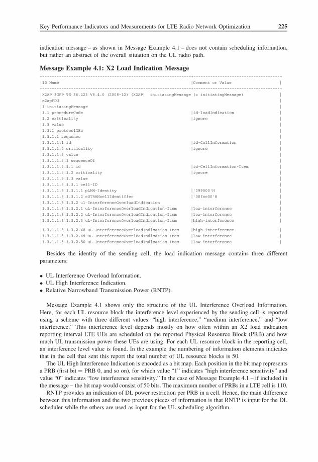
indication message – as shown in Message Example 4.1 – does not contain scheduling information,but rather an abstract of the overall situation on the UL radio path.
Message Example 4.1: X2 Load Indication Message+--------------------------------------------------------------+------------------------------------+
|ID Name |Comment or Value |
+--------------------------------------------------------------+------------------------------------+
|X2AP 3GPP TS 36.423 V8.4.0 (2008-12) (X2AP) initiatingMessage (= initiatingMessage) |
|x2apPDU |
|1 initiatingMessage |
|1.1 procedureCode |id-loadIndication |
|1.2 criticality |ignore |
|1.3 value |
|1.3.1 protocolIEs |
|1.3.1.1 sequence |
|1.3.1.1.1 id |id-CellInformation |
|1.3.1.1.2 criticality |ignore |
|1.3.1.1.3 value |
|1.3.1.1.3.1 sequenceOf |
|1.3.1.1.3.1.1 id |id-CellInformation-Item |
|1.3.1.1.3.1.2 criticality |ignore |
|1.3.1.1.3.1.3 value |
|1.3.1.1.3.1.3.1 cell-ID |
|1.3.1.1.3.1.3.1.1 pLMN-Identity |'299000'H |
|1.3.1.1.3.1.3.1.2 eUTRANcellIdentifier |'00fce00'H |
|1.3.1.1.3.1.3.2 ul-InterferenceOverloadIndication |
|1.3.1.1.3.1.3.2.1 uL-InterferenceOverloadIndication-Item |low-interference |
|1.3.1.1.3.1.3.2.2 uL-InterferenceOverloadIndication-Item |low-interference |
|1.3.1.1.3.1.3.2.3 uL-InterferenceOverloadIndication-Item |high-interference |
|1.3.1.1.3.1.3.2.48 uL-InterferenceOverloadIndication-Item |high-interference |
|1.3.1.1.3.1.3.2.49 uL-InterferenceOverloadIndication-Item |low-interference |
|1.3.1.1.3.1.3.2.50 uL-InterferenceOverloadIndication-Item |low-interference |
Besides the identity of the sending cell, the load indication message contains three differentparameters:
• UL Interference Overload Information.• UL High Interference Indication.• Relative Narrowband Transmission Power (RNTP).
Message Example 4.1 shows only the structure of the UL Interference Overload Information.Here, for each UL resource block the interference level experienced by the sending cell is reportedusing a scheme with three different values: “high interference,” “medium interference,” and “lowinterference.” This interference level depends mostly on how often within an X2 load indicationreporting interval LTE UEs are scheduled on the reported Physical Resource Block (PRB) and howmuch UL transmission power these UEs are using. For each UL resource block in the reporting cell,an interference level value is found. In the example the numbering of information elements indicatesthat in the cell that sent this report the total number of UL resource blocks is 50.
The UL High Interference Indication is encoded as a bit map. Each position in the bit map representsa PRB (first bit = PRB 0, and so on), for which value “1” indicates “high interference sensitivity” andvalue “0” indicates “low interference sensitivity.” In the case of Message Example 4.1 – if included inthe message – the bit map would consist of 50 bits. The maximum number of PRBs in a LTE cell is 110.
RNTP provides an indication of DL power restriction per PRB in a cell. Hence, the main differencebetween this information and the two previous pieces of information is that RNTP is input for the DLscheduler while the others are used as input for the UL scheduling algorithm.

226 LTE Signaling, Troubleshooting and Optimization
Again, RNTP is reported as a bit map. Each position in the bitmap represents a PRB value (i.e.,first bit = PRB 0, and so on). Instead of the full bit map the value 0 might be transmitted to indicate“Tx not exceeding RNTP threshold” or value 1 indicates “no promise on the Tx power is given”by the reporting cell. The individual RNTP threshold values for the PRBs are encoded as an integernumber covering the range from −11 to +3 dB.
Regarding aggregation and visualization of the X2 load indication measurements – and the samestatement is true for the PRB usage reports discussed in the next section – it is obvious that simplecounter or histogram data is an inapplicable approach. The best way to visualize what is periodicallyreported using bit maps is what was shown in Figure 4.7.
4.2.3 The eNodeB Layer 2 Measurements
The measurements described in this chapter are defined in 3GPP 36.314. The intention of this standarddocument is to define some common statistics for radio interface performance and in some cases togenerate measurements to serve the X2 load indication reporting.
4.2.3.1 PRB Usage
The usage of PRBs can be reported by the eNB (to, for example, the Operation and MaintenanceCenter (OMC)) for UL and DL in a particular cell in different flavors:
1. UL/DL total PRB usage: The objective of the PRB usage measurements is to measure the useof time and frequency resources. One use case is cell load balancing, where PRB usage relates toinformation signaled across the X2 interface. Another use case is O&M performance observability.
2. UL/DL PRB usage per traffic class: This measurement is an aggregate for all UEs in a cell,and is applicable to Dedicated Traffic Channels (DTCHs). The reference point is the SAP betweenMAC and L1. The measurement is done separately for DL DTCH, for each QCI, and UL DTCH,for each CQI.
3. UL/DL PRB usage per Signaling Radio Bearer (SRB): This measurement is applicable to Ded-icated Control Channels (DCCHs). The reference point is the SAP between MAC and L1. Themeasurement is done separately for DL DCCH and UL DCCH.
4. DL PRB usage for Common Control Channels (CCCHs): This measurement is applicable tothe Broadcast Control Channel (BCCH) and Paging Control Channel (PCCH). The reference pointis the SAP between MAC and L1.
5. UL PRB usage for CCCHs: This is the percentage of PRBs used for CCCHs’ Random AccessChannel (RACH) and Physical Uplink Control Channel (PUCCH). Value range: 0–100%.
Basically, all PRB usage statistics can also be visualized using a radio interface tester as shown inFigure 4.7. The reporting format on the O&M interface between the eNB and OMC is not defined ininternational standards and, hence, is of proprietary nature. However, due to the limited processingresources available in the eNB for performance measurement and statistical tasks, it can be guessedthat what is provided to the OMC is also rather highly aggregated in the time and maybe also frequencydimension. Compared to what can be measured and visualized using a radio interface tester, the OMCstatistics may be sufficient to determine the average load in a cell on an hourly or 15 minute basis.These will not help to verify and optimize the scheduling algorithms as a radio interface tester can do.
4.2.3.2 Received Random Access Preamble
The number of received random access preambles is an important accessibility KPI for a cell. Themore preambles the UE must send to get RACH resources assigned by the cell, the longer it takes to

Key Performance Indicators and Measurements for LTE Radio Network Optimization 227
Figure 4.15 Number of active UEs (“users”) over time.
set up a call or to complete a handover to an E-UTRAN target cell. The worst cell is the cell withthe highest number of received random access preambles. In the worst case the UE never gets accessto the RACH – an effect that is known from drive test campaigns as the “sleeping cell.”
As a result, it emerges that received random access preambles is a very important measurement,but experience with RAN vendors in 3G UTRAN has proven that this measurement (which also existsfor UTRAN cells) was never enabled. If this will change in LTE RAN is a question that cannot beanswered at the time this chapter was being written (winter 2009).
4.2.3.3 Number of Active UEs
The number of active UEs is a simple gauge measurement that shows how many subscribers onaverage use the resources of the cell over a defined period of time.
This measurement is important for traffic and radio resource planning. It depends on the individualoptimization task and which granularity is necessary on the time axis. Typical reporting intervals ofOMC statistics are 15, 30, and 60 minutes. However, looking at Figure 4.15, which shows a muchbetter time granularity, the peaks in subscriber activity (in the figure up to approximately 25, whilethe average value for 15 or 30 minutes could be something around 12–15) that may lead to a shortageof radio resources in the cell can be clearly identified.
4.3 Radio Quality Measurements
There is a set of radio quality measurements specified by 3GPP. In particular, the definitions can befound in 3GPP 36.214 “E-UTRA Physical Layer Measurements.” These measurements are split intoE-UTRAN measurements that are provided by the eNB and UE measurements reported by the handset.Especially for the E-UTRAN measurements, the 3GPP standards must be seen as an option and thereis no guarantee that eNB vendors will implement them. In any case there is room for proprietaryimplementations, because there are no standardized measurement reports defined for the S1 interface.It is expected that in most cases the E-UTRAN measurement results will be sent to the OMC viaO&M interfaces using a proprietary protocol. Also, the binning of E-UTRAN measurements is – incontrast to the 3G UTRAN standards – not defined by 3GPP.
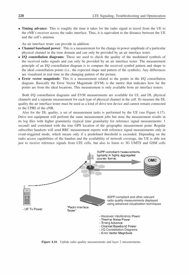
The radio quality measurements can be split into UL and DL measurements. Looking at the ULmeasurements illustrated in Figure 4.16, the only measurement sent by the UE using a RRC mea-surement report is the UE Tx power, the power used by the handset to send the physical UL signaltoward the eNB.
On the eNB side the following parameters can be measured by the base station:
• Received Interference Power (RIP): This is the UL noise floor for a set of UL resource blocks.• Thermal noise power: This is the UL noise for the entire UL frequency bandwidth of the receiving
cell without the signals received from LTE handsets.
228 LTE Signaling, Troubleshooting and Optimization
• Timing advance: This is roughly the time it takes for the radio signal to travel from the UE tothe eNB’s receiver across the radio interface. Thus, it is equivalent to the distance between the UEand the cell’s antenna.
An air interface tester can provide in addition:• Channel baseband power: This is a measurement for the change in power amplitude of a particular
physical channel in the time domain and can only be provided by an air interface tester.• I/Q constellation diagrams: These are used to check the quality of the modulated symbols of
the received radio signals and can only be provided by an air interface tester. The measurementprinciple of an I/Q constellation diagram is to compare the received symbol pattern and shape tothe ideal constellation points (i.e., the expected shape and pattern of the symbols). Any differencesare visualized in real time in the changing pattern of the picture.
• Error vector magnitude: This is a measurement related to the points in the I/Q constellationdiagram. Basically the Error Vector Magnitude (EVM) is the metric that indicates how far thepoints are from the ideal locations. This measurement is only available from air interface testers.
Both I/Q constellation diagrams and EVM measurements are available for UL and DL physicalchannels and a separate measurement for each type of physical channel in the cell. To measure the DLquality the air interface tester must be used as a kind of drive test device and cannot remain connectedto the CPRI of the eNB.
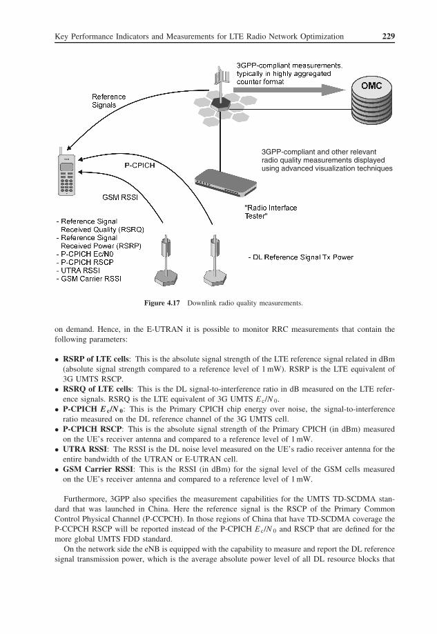
Also for the DL quality, a set of measurement tasks is performed by the UE (see Figure 4.17).Drive test equipment will perform the same measurement jobs but store the measurement results inits log files with higher granularity (typical time granularity for reference signal measurements: 1second) and correlated with the true GPS location of the geographic measurement point. Regularsubscriber handsets will send RRC measurement reports with reference signal measurements only inevent-triggered mode, which means only if a predefined threshold is exceeded. Depending on theradio access capabilities of the handset and the availability of network coverage, the UE is able notjust to receive reference signals from LTE cells, but also to listen to 3G UMTS and GSM cells
3GPP-compliant and other relevantradio quality measurements displayedusing advanced visualization techniques
I/Q Constellation Diagrams
Figure 4.16 Uplink radio quality measurements and layer 2 measurements.
Key Performance Indicators and Measurements for LTE Radio Network Optimization 229
3GPP-compliant and other relevantradio quality measurements displayedusing advanced visualization techniques
Figure 4.17 Downlink radio quality measurements.
on demand. Hence, in the E-UTRAN it is possible to monitor RRC measurements that contain thefollowing parameters:
• RSRP of LTE cells: This is the absolute signal strength of the LTE reference signal related in dBm(absolute signal strength compared to a reference level of 1 mW). RSRP is the LTE equivalent of3G UMTS RSCP.
• RSRQ of LTE cells: This is the DL signal-to-interference ratio in dB measured on the LTE refer-ence signals. RSRQ is the LTE equivalent of 3G UMTS E c/N 0.
• P-CPICH E c/N 0: This is the Primary CPICH chip energy over noise, the signal-to-interferenceratio measured on the DL reference channel of the 3G UMTS cell.
• P-CPICH RSCP: This is the absolute signal strength of the Primary CPICH (in dBm) measuredon the UE’s receiver antenna and compared to a reference level of 1 mW.
• UTRA RSSI: The RSSI is the DL noise level measured on the UE’s radio receiver antenna for theentire bandwidth of the UTRAN or E-UTRAN cell.
• GSM Carrier RSSI: This is the RSSI (in dBm) for the signal level of the GSM cells measuredon the UE’s receiver antenna and compared to a reference level of 1 mW.
Furthermore, 3GPP also specifies the measurement capabilities for the UMTS TD-SCDMA stan-dard that was launched in China. Here the reference signal is the RSCP of the Primary CommonControl Physical Channel (P-CCPCH). In those regions of China that have TD-SCDMA coverage theP-CCPCH RSCP will be reported instead of the P-CPICH E c/N 0 and RSCP that are defined for themore global UMTS FDD standard.
On the network side the eNB is equipped with the capability to measure and report the DL referencesignal transmission power, which is the average absolute power level of all DL resource blocks that

230 LTE Signaling, Troubleshooting and Optimization
are used to send reference signals. This value is equivalent to the P-CPICH Tx power that was notmeasured in 3G UMTS cells, but configured as a fix value during cell setup or reset.
4.3.1 UE Measurements
4.3.1.1 RSRP
RSRP is used to measure the coverage of the LTE cell on the DL. The UE will send RRC measurementreports that include RSRP values in a binned format. The appropriate bin mapping is given in Table 4.1.The reporting range of RSRP is defined from −140 to −44 dBm with 1 dB resolution.
The main purpose of RSRP is to determine the best cell on the DL radio interface and select thiscell as the serving cell for either initial random access or intra-LTE handover. The RRC measurementreports with RSRP measurement results will be sent by the UE if a predefined event trigger criterionis met (see Section 1.10.8.3).
There is certainly a correlation also between RSRP and the user plane QoS. As a rule of thumb fora cell in the outdoor environment, the RSRP measurement results can be categorized in three ranges.If RSRP > −75 dBm, excellent QoS can be expected as long as not too many subscribers struggle forthe available bandwidth of the cell. In the range between −75 and −95 dBm a slight degradation ofthe QoS can be expected, for example, throughput will decline by 30–50% if RSRP goes down from−75 to −95 dBm. Below −95 dBm the QoS become unacceptable and throughput tends to declinedown to zero at approximately −108 to −100 dBm. Under such radio conditions, call drops must beexpected as the worst case.
Due to their limited footprint, in-house cells are normally able to deal with radio conditions thatare worse compared to what is measured in the outdoor environment. Consequently, an acceptableQoS for RSRP values as low as −115 dBm can be assumed, based on what was observed in the 3GUTRAN environment for CPICH RSCP.
4.3.1.2 RSRQ
Like RSRP, RSRQ is used to determine the best cell for LTE radio connection at a certain geographiclocation. However, while RSRP is the absolute strength of the reference radio signals, RSRQ isthe signal-to-noise ratio. Like RSRP, RSRQ can be used as the criterion for initial cell selectionor handover.
Simply, the calculation of RSRQ can be expressed by the following formula:
RSRQ[dB] = 10lgRSRP
RSSI(4.1)
Table 4.1 RSRP measurement report mapping.Reproduced with permission from © 3GPP™
Reported value Measured quantity value Unit
RSRP_00 RSRP < −140 dBmRSRP_01 –140 ≤ RSRP < −139 dBmRSRP_02 –139 ≤ RSRP < −138 dBm
. . . . . . . . .
RSRP_95 –46 ≤ RSRP < −45 dBmRSRP_96 –45 ≤ RSRP < −44 dBmRSRP_97 –44 ≤ RSRP dBm

Key Performance Indicators and Measurements for LTE Radio Network Optimization 231
Figure 4.18 LTE coverage and interference problems.
The reporting range of RSRQ is defined from −19.5 to −3 dB with 0.5 dB resolution (Table 4.2).When comparing the measurement results of RSRQ and RSRP that have been made at the same
geographic location – in a protocol trace they can be identified by the same timestamp – it is possible todetermine if coverage or interference problems occur at this location. This is illustrated in Figure 4.18.
If a UE changes its location or if radio conditions change due to other reasons and RSRP (i.e., theabsolute signal strength of the reference signals) remains stable or becomes even better than before
Table 4.2 RSRQ measurement report mapping.Reproduced with permission from © 3GPP™
Reported value Measured quantity value Unit
RSRQ_00 RSRQ < −19.5 dBRSRQ_01 –19.5 ≤ RSRQ < −19 dBRSRQ_02 –19 ≤ RSRQ < −18.5 dB
. . . . . . . . .
RSRQ_32 –4 ≤ RSRQ < −3.5 dBRSRQ_33 –3.5 ≤ RSRQ < −3 dBRSRQ_34 –3 ≤ RSRQ dB

232 LTE Signaling, Troubleshooting and Optimization
while RSRQ is declining, this is an unambiguous symptom of rising interference. If, on the otherhand, both RSRP and RSRQ decline at the same time/location, this clearly indicates an area withweak coverage. This kind of evaluation is very important for finding the root cause of call drops dueto radio problems.
Similar to what was described for RSRP, for RSRQ also three quality ranges can be defined, but thenumbers here are still very uncertain since no loaded network environment has yet been monitored,due to the fact that the number of calls and location of subscribers are limited during field trials. All inall, it seems that in general RSRQ values higher than −9 dB guarantee the best subscriber experience.The range between −9 and −12 dB can be seen as neutral with a slight degradation of QoS, butoverall customer experience is still at a fair level. Starting with RSRQ values of −13 dB and lower,things become worse with significant declines of throughput and a high risk of call drop.
4.3.1.3 Power Headroom
The Power Headroom (PH), expressed in decibels, is defined as the difference between the nominal UEmaximum transmit power and the estimated power for the Physical Uplink Shared Channel (PUSCH)transmission. It is the power that can be added to UL data transmission if the UE moves toward thecell edge or requires a service with a higher guaranteed bit rate.
The PH reporting interacts with the UL scheduling function of the eNB. The reports can be senteither event triggered or periodically. An event is triggered if, after a period of not allowed PHreporting, the appropriate timer in the UE expires, if the path loss change is higher than a prede-fined value. Otherwise, periodic PH reporting starts with configuration or reconfiguration of the PHmeasurement task.
The PH reports are send on the MAC layer, not in RRC measurement reports! However, theeNB is able to control the UE’s maximum UL transmission power using the P-max parameter inRRC signaling.
The PH reporting range is from −23 to +40 dB. Table 4.3 defines the mapping for the report inbinned format. The 64 possible values correspond to 6 bits of the PH control element in the MACprotocol definitions.
Table 4.3 Power headroom bin mapping table.Reproduced with permission from © 3GPP™
Reported value Measured quantityvalue (dB)
POWER_HEADROOM_0 –23 ≤ PH < −22POWER_HEADROOM_1 –22 ≤ PH < −21POWER_HEADROOM_2 –21 ≤ PH < −20POWER_HEADROOM_3 –20 ≤ PH < −19POWER_HEADROOM_4 –19 ≤ PH < −18POWER_HEADROOM_5 –18 ≤ PH < −17
. . . . . .
POWER_HEADROOM_57 34 ≤ PH < 35POWER_HEADROOM_58 35 ≤ PH < 36POWER_HEADROOM_59 36 ≤ PH < 37POWER_HEADROOM_60 37 ≤ PH < 38POWER_HEADROOM_61 38 ≤ PH < 39POWER_HEADROOM_62 39 ≤ PH < 40POWER_HEADROOM_63 PH ≥ 40

Key Performance Indicators and Measurements for LTE Radio Network Optimization 233
Figure 4.19 UL scheduling for four different UEs in same cell.
Since the PH reporting is not foreseen as an eNB statistical value to be reported via a northboundinterface, it can only be analyzed and visualized by using a radio interface protocol tester.
4.3.1.4 UL Scheduling Requests
The UL scheduling request is used for requesting Uplink Shared Channel (UL-SCH) resources for newtransmission. This is also not a measurement for statistical purposes, but mandatory for troubleshootingand optimizing the UL scheduling function of the eNB.
UL scheduling requests are sent on the MAC layer and can be tracked for measurement purposesby an air interface tester and visualized as shown in Figure 4.19. There are no scheduling requeststatistics provided by the eNB.
4.3.1.5 Buffer Status Reporting
Another important input for the UL scheduling that is also sent on the MAC layer is the UL bufferstatus report of the UE. It is used the inform the serving eNB about the amount of data waiting fortransmission in the UL buffers of the UE.
The Buffer Status Reports (BSRs) are either sent periodically or event triggered. Typical eventtriggers are the following:
• UL data for a logical channel which belongs to a logical channel group becomes available fortransmission in the Radio Link Control (RLC) or PDCP entity.
• UL resources are allocated and the UE detects that the number of padding bits is equal to or largerthan the size of the BSR MAC control element. In such a case the BSR is called a Padding BufferStatus Report.

234 LTE Signaling, Troubleshooting and Optimization
• A serving cell change occurs or the retransmission timer for BSRs expires while the UE has datawaiting for UL transmission. Here the 3GPP specs use the name “Regular Buffer Status Report.”A Regular Buffer Status Report to be sent to the eNB should trigger an UL scheduling request tobe sent in parallel.
It is also necessary to distinguish between long and short BSRs (compare Figure 4.20 to Figure 4.21).The long report format is used if more than one logical channel group has data available for ULtransmission in the TTI where the BSR is transmitted. In any other case, the short format is used.
For the reporting a binned format (index) is used as defined in Table 4.4. Like other UE measure-ments reported on the MAC layer, there are no statistics for BSRs from the eNB defined by 3GPP.Hence, the availability of measurement results for troubleshooting and network optimization relies onproprietary implementations and the radio interface test equipment.
4.3.2 The eNodeB Physical Layer Measurements
4.3.2.1 Received Interference Power (RIP)
This is the UL noise floor for a set of UL resource blocks. Typically the UL noise is generated bythe UL signals of all UEs received in the particular frequency range of these resource blocks on asingle Rx antenna. The measurement is defined by 3GPP to be implemented in the eNB, but can alsobe provided by an air interface tester that is connected to the eNB’s CPRI.
The reporting range for RIP is from −126 to −75 dBm. The values are reported in binned formataccording to the definitions in Table 4.5.
Besides the UL load in the cell that is determined by the number of active subscribers, the excep-tional values of RIP can also be caused by high-frequency signal sources outside the LTE radionetwork. In 3G UMTS networks typical sources of interfering high-frequency signals have been iden-tified as old-fashioned DECT phones, radar systems of airports and ships, and amplifiers of satellitedishes used to receive sat TV at home. The same kind of interference caused by external signal sourcescan be expected to be found also in LTE cells, but as shown in Figure 4.22 the impact on the LTEcell is much less dramatic compared to what happens in the UMTS cell.
In UMTS if a single sideband of an external high-frequency signal source strikes the UL or DLfrequency band of the cell with a certain power the entire bandwidth of the cell is impacted and
Figure 4.20 Short buffer status MAC control element. Reproduced with permission from © 3GPP™.
Figure 4.21 Long buffer status MAC control element. Reproduced with permission from © 3GPP™.

Key Performance Indicators and Measurements for LTE Radio Network Optimization 235
Table 4.4 BSR bin mapping table. Reproduced with permission from © 3GPP™
Index Buffer Size (BS) Index BS valuevalue (bytes) (bytes)
0 BS = 0 32 1132 < BS ≤ 13261 0 < BS ≤ 10 33 1326 < BS ≤ 15522 10 < BS ≤ 12 34 1552 < BS ≤ 18173 12 < BS ≤ 14 35 1817 < BS ≤ 21274 14 < BS ≤ 17 36 2127 < BS ≤ 24905 17 < BS ≤ 19 37 2490 < BS ≤ 29156 19 < BS ≤ 22 38 2915 < BS ≤ 34137 22 < BS ≤ 26 39 3413 < BS ≤ 39958 26 < BS ≤ 31 40 3995 < BS ≤ 46779 31 < BS ≤ 36 41 4677 < BS ≤ 547610 36 < BS ≤ 42 42 5476 < BS ≤ 641111 42 < BS ≤ 49 43 6411 < BS ≤ 750512 49 < BS ≤ 57 44 7505 < BS ≤ 878713 57 < BS ≤ 67 45 8787 < BS ≤ 10 28714 67 < BS ≤ 78 46 10 287 < BS ≤ 12 04315 78 < BS ≤ 91 47 12 043 < BS ≤ 14 09916 91 < BS ≤ 107 48 14 099 < BS ≤ 16 50717 107 < BS ≤ 125 49 16 507 < BS ≤ 19 32518 125 < BS ≤ 146 50 19 325 < BS ≤ 22 62419 146 < BS ≤ 171 51 22 624 < BS ≤ 26 48720 171 < BS ≤ 200 52 26 487 < BS ≤ 31 00921 200 < BS ≤ 234 53 31 009 < BS ≤ 36 30422 234 < BS ≤ 274 54 36 304 < BS ≤ 42 50223 274 < BS ≤ 321 55 42 502 < BS ≤ 49 75924 321 < BS ≤ 376 56 49 759 < BS ≤ 58 25525 376 < BS ≤ 440 57 58 255 < BS ≤ 68 20126 440 < BS ≤ 515 58 68 201 < BS ≤ 79 84627 515 < BS ≤ 603 59 79 846 < BS ≤ 93 47928 603 < BS ≤ 706 60 93 479 < BS ≤ 109 43929 706 < BS ≤ 826 61 10 9439 < BS ≤ 128 12530 826 < BS ≤ 967 62 12 8125 < BS ≤ 150 00031 967 < BS ≤ 1132 63 BS > 150 000
Table 4.5 Received interference power – reporting range andbin mapping table. Reproduced with permission from © 3GPP™
Reported value Measured quantity Unitvalue
RTWP_LEV _000 RIP < −126.0 dBmRTWP_LEV _001 –126.0 ≤ RIP < −125.9 dBmRTWP_LEV _002 –125.9 ≤ RIP < −125.8 dBm
. . . . . . . . .
RTWP_LEV _509 –75.2 ≤ RIP < −75.1 dBmRTWP_LEV _510 –75.1 ≤ RIP < −75.0 dBmRTWP_LEV _511 –75.0 ≤ RIP dBm

236 LTE Signaling, Troubleshooting and Optimization
sidebandinterferencein UMTS DL
sidebandinterference inLTE frequencyband
UMTS ULf1
(5 MHz)
UMTS DLf2
(5 MHz)
Figure 4.22 Impact of external interference in UMTS and LTE cells.
in the worst case the cell becomes unusable for transmission of UMTS radio signals, because allconnections are distributed over the entire frequency band and diversity between different connectionsis only available in the power domain (amplitude of UMTS signals). In LTE the scheduling grid thatgives diversity in both the frequency and time domains reduces the impact of the interfering sidebandto a minimum. If the interfering carrier is permanently present, no more than just a few subframes ofthe entire frequency band become unusable and in the case of, for example, radar beams that strikethe cell with a certain periodicity, the impact on the subcarriers is further limited to a few sub-slotsof a particular frequency in the time domain.
All in all, this comparison shows that LTE is much less interference sensitive than UMTS FDDand, hence, it can be expected that also “interference hunting” will have much less importance duringthe deployment phase of the networks compared to what was done during UMTS FDD rollout.
4.3.2.2 Thermal Noise Power
This is the UL noise for the entire UL frequency bandwidth of the receiving cell without the signalsreceived from LTE handsets. So it is the UL noise without the LTE traffic. The measurement isoptionally provided by the eNB and can also be provided by a radio interface tester.
4.3.2.3 Timing Advance
Actually the timing advance is not measured for the purpose of statistics. Rather it is required tosynchronize the transmission and reception of UL radio signals between the UE and eNB in the timedomain of the air interface. The timing advance is the estimated time that a particular UL subframeneeds to travel from the UE’s Tx antenna to the cell’s Rx antenna. This is illustrated in Figure 4.23where three different UEs have been scheduled for the same UL sub-slot on the time domain, but dueto the fact that the distance between the UE and receiving cell is different for each handset, the radiosignal of UE3 needs three times more time to travel all the way from the UE to the cell. Hence, theUL signal of UE3 must be sent earlier compared to the signal of UE1 if both signals are to arrive atthe same sub-slot of the time domain in the cell. By sending the timing advance command the eNBadjusts the proper arrival time of all three UL radio signals individually.
The initial timing advance command is sent together with the random access response encoded inan 11-bit timing advance value T A. The 11 bits defines a range of possible random access timing

Key Performance Indicators and Measurements for LTE Radio Network Optimization 237
Figure 4.23 Timing advance principle.
advance values represented by integer index values of T A = 0, 1, 2, . . . , 1282. The step size of thetiming advance value is expressed in multiples of 16Ts , where Ts is the basic time unit of the LTEradio interface and defined in 3GPP 36.211 as follows:
Ts = 1/ (15000 × 2048) s = 1/30720000 s = 32.552083 ns
Thus, one step timing advance (T A) in the time domain of the radio signal is
TA = 16Ts = 16 × 32.552083 ns = 0.52 μs
Considering that the radio waves travel at speed of light c or 300 000 km/s, the geographic distancefor a single timing advance step can be calculated using the following formula where r represents theradius of the cell at a distance equal to T A:
r = c × 16Ts = 300 m × 0.52 = 156 m
If the maximal timing advance index value of 1282 is seen during the random access response,this means that the UE is 1282 × 156 m = 199 992 m (roughly 200 km) away from the cell’s antennawhen sending the random access preamble.
After establishment of the RRC connection the 6-bit timing advance values are sent on the MAClayer using the Physical Downlink Shared Channel (PDSCH) whenever the distance between the UEand cell changes significantly. The 6-bit field allows a range of MAC timing advance command valuesbetween 0 and 63. These timing advance command values sent during the active call are relative tothe current UL timing, which means that they do not correspond to the total distance between the UEand cell, but only to the change in distance since the last timing advance command was sent.
Thus, whenever a UE receives a timing advance command from the eNB, it needs to calculate thenew timing advance using the formula
NTA,new = NTA,old + (TA − 31) × 16
The best possible granularity for timing advance commands is 2 Hz – when a new timing advancecommand is sent every 500 ms. Using the 64 index values, a distance of 64 × 156 m = 9984 m(roughly 10 km) is covered and, hence, the timing advance can be properly adjusted when the UEchanges its position relative to the eNB by ±5 km within 500 ms. Theoretically this would be sufficientin cases where the UE moves at 3600 km/h. However, it must be taken into account that changes in

238 LTE Signaling, Troubleshooting and Optimization
the air interface radio way are not just due to subscriber mobility, but also the longer ways in the airdue to reflection of radio signals, especially in city center environments like New York City.
It should also be noted that there is a delay between the reception and execution of a timing advancecommand inside the UE. Normally a timing advance command received at the UE is executed for theUL subframe that begins six subframes later. Errors in timing advance measurement, transmission,and execution will cause in the worst case the loss of UL radio frames, which seriously deterioratesthe user’s quality of experience, especially for real-time services like Voice over IP (VoIP). To detectdefects in the timing advance procedure these measurements should not just be measured per call,but also collected in an aggregated format per handset type and cell to benchmark the equipment ofdifferent UE manufacturers and cells that cover different geographic areas against each other. Besidescorrelation with UL radio quality measurements, the timing advance information can also be helpfulin estimating the UE’s geographic position in cases when GPS methods are not available.
The timing advance measurements are not defined by 3GPP as part of the eNB statistical mea-surements. Rather it is a task for a protocol tester to decode and store the timing advance commandvalues in a trace file. It is possible to capture the timing advance commands directly on the radiosignal stream that is monitored at the CPRI. Alternatively, eNBs may have a monitoring port to allowthe capture of radio protocol traces.
4.3.3 Radio Interface Tester Measurements
4.3.3.1 Channel Baseband Power
The channel baseband power measurement is used to track the changes in the power amplitude ofphysical channels over time. This measurement is available for both the receiver and transmitter sidesof a particular physical channel. Thus, in an ideal measurement scenario a radio interface tester shouldbe located at each side of the connection, at the UE and eNB.
Under these conditions the baseband power measurements for all physical channels are availablein a graphical format as shown in Figure 4.24. In particular, these measurements are used to evaluatethe amplitude of sent and received signals for the:
• Physical Downlink Shared Channel (PDSCH).• Physical Downlink Control Channel (PDCCH).• Primary Synchronization Channel (P-SCH).• Secondary Synchronization Channel (S-SCH).• Physical Broadcast Channel (PBCH).• Physical Uplink Shared Channel (PUSCH).• Physical Uplink Control Channel (PUCCH).
4.3.4 I/Q Constellation Diagrams
A constellation diagram is a scatter diagram used to visualize the distribution of symbols of a modulatedsignal in the so-called complex plane. For each common modulation scheme such as Phase ShiftKeying (PSK) and Quadrature Amplitude Modulation (QAM) the ideal distribution pattern of symbolsin the complex plane is known from signal theory. Now the measured pattern can be visually comparedto the expected ideal pattern.
In the ideal pattern each symbol dot is laser focused on a particular fixed position of the constellationdiagram. The real-time measurement as shown in Figure 4.25 shows the symbol measurement samples“dancing” around their ideal positions and the further they are from the ideal position as plotted, themore the signal was corrupted.

Key Performance Indicators and Measurements for LTE Radio Network Optimization 239
Figure 4.24 Channel baseband power measurement graph.
Figure 4.25 Two-dimensional I/Q constellation diagram.
240 LTE Signaling, Troubleshooting and Optimization
For the purpose of analyzing received signal quality, some types of corruption are very evident inthe constellation diagram. Typical radio transmission problems can be easily recognized as follows:
• Gaussian noise becomes evident as fuzzy constellation points.• Non-coherent single frequency interference manifests as circular constellation points.• Phase noise leads to rotationally spreading constellation points.• Amplitude compression causes the corner points to move toward the center.
The I/Q constellation diagram can be measured on the transmitter side – then it shows the quality ofsignal modulation before transmission over the air interface. However, this use case is seen more in thelab than in live networks. The typical use case for live networks is to measure the modulation qualityof a received signal. A high-quality air interface tester should provide the particular I/Q constellationdiagrams for the following physical channels:
• Physical Downlink Shard Channel (PDSCH).• Physical Downlink Control Channel (PDCCH).• Primary Synchronization Channel (P-SCH).• Secondary Synchronization Channel (S-SCH).• Physical Broadcast Channel (PBCH).• Physical Uplink Shared Channel (PUSCH).• Physical Uplink Control Channel (PUCCH).• Sounded Reference Symbols (SRSs) for UL.
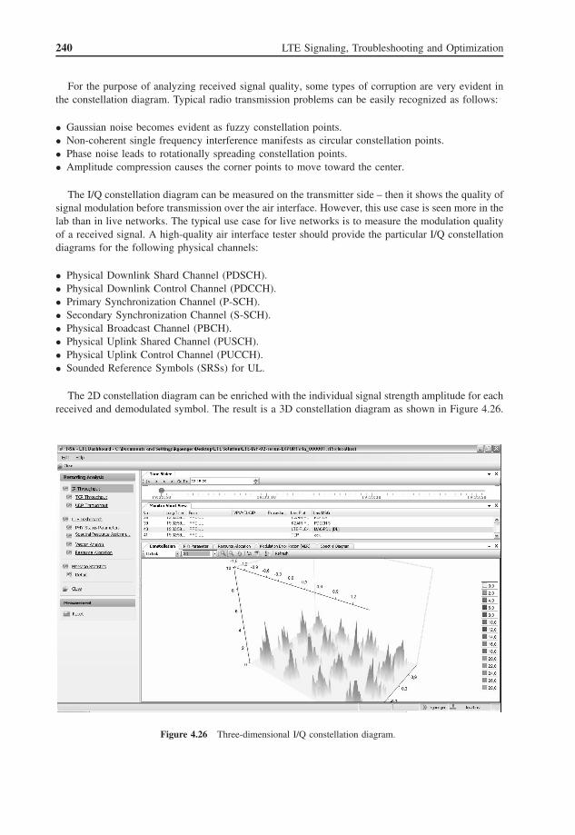
The 2D constellation diagram can be enriched with the individual signal strength amplitude for eachreceived and demodulated symbol. The result is a 3D constellation diagram as shown in Figure 4.26.
Figure 4.26 Three-dimensional I/Q constellation diagram.

Key Performance Indicators and Measurements for LTE Radio Network Optimization 241
4.3.5 EVM/Modulation Error Ratio
The EVM is sometimes also called the Receive Constellation Error (RCE). It is a measurement usedto express the difference between measured constellation points and the ideal constellation point inthe complex plane; in other words, how far the measured points are from the ideal location.
Like I/Q constellation diagrams, the EVM can be measured with radio interface testers and cannotbe provided by any drive test or eNB statistics.
The principle of determining the EVM is shown in Figure 4.27. Due to radio transmission error,the measured constellation point drifted away from the ideal location and, starting from the center ofthe I/Q constellation diagram, a power vector for each point – ideal and measured – can be calculated.These vectors are P error and P reference.
To compute the EVM, P error and P reference are set in relation to each other so that the EVM is theratio of the power of the error vector to the root mean square of the reference power. The result canbe expressed as a percentage when using Equation 4.1:
EVM(%) =√
Perror
Preference× 100% (4.2)
The measurement can also be defined in decibels when Equation 4.2 is used with identical valuesfor error vector power and reference vector power:
EVM(dB) = 10 log10
(Perror
Preference
)(4.3)
Now, within LTE cells the power and modulation scheme assigned to particular subcarriers overtime may change frequently and, to give an overview of the radio transmission quality of the entirefrequency spectrum, an aggregation of measurement results is required. The aggregated view withone MER (Modulation Error Ratio) bar for each subcarrier of the frequency spectrum is shown inFigure 4.28. By filtering on radio frames belonging to a particular UE it is even possible to visualizein this view the changes in EMV/MER during a single call.
Figure 4.27 Measurements to compute EVM/MER.

242 LTE Signaling, Troubleshooting and Optimization
Figure 4.28 Modulation error ratio for LTE spectrum.
4.4 Control Plane Performance Counters and Delay Measurements
A set of common performance counters for accessibility, retainability, and mobility KPIs is generatedby network elements like eNB and MME. Hence, these performance counters are also named networkelement counters or OMC counters.
The disadvantage of such network element counters is that their trigger point definitions often fol-low proprietary standards so that, for example, a set of Nokia Siemens Network MME counters willnever be 100% identical to a set from an Ericsson MME. And the differences are growing in the fieldof KPI formula definition that is in large portions not covered by any international standard althougha comprehensive set of KPIs for the E-UTRAN is defined in 3GPP 32.450. This set of standard KPIsis quite sophisticated and almost impossible to be implemented by external measurement equipment,because check of user plane buffer status is mandatory and external measurement equipment can-not check the user plane buffer inside the network elements. However, even implementation insidethe network element is not easy and significant processing resources are required to compute suchsophisticated KPIs in the network elements. For this reason NEMs will hesitate to move forwardwith the implementation as proposed by 3GPP. Also, any network element performance counters areaggregated at a single measurement point and do not provide end-to-end visibility, which means thatif a failure is found in eNB statistics it might be possible to determine that the origin of this failurewas not in the eNB itself, but somewhere in the core network. However, it is impossible to see fromthe eNB that the root cause of a core network problem that triggered a chain reaction including failurein the eNB was located in the Public Data Network Gateway (PDN-GW). To follow a call acrossmultiple interfaces, synchronize the timestamps of measurements and protocol events, and providea single user access point for data analysis are the job of a classical network management system.Although it is not easy to give a clear definition of a “call” in the all-IP world of LTE and EPC, thegeneral measurement tasks and aggregation levels are almost the same as in earlier 2G/3G networks.
It is also clear that the air interface measurements that have been discussed in the previous sectionsin deployment scenarios with 300–6000 eNBs connected to a single MME cannot be expected to be

Key Performance Indicators and Measurements for LTE Radio Network Optimization 243
available from all base stations of a network at any time. Nor is it technically required to monitor,for example, the scheduler efficiency for all sites 24/7; neither does it make sense from a cost-per-siteperspective when it is considered that already a single air interface tester is more expensive than acomplete eNB with its hardware and software. Further, it would be necessary to build an architecturethat allows access to all air interface measurement data from a single user access point.
Knowing these limitations, the optimal way to troubleshoot and optimize the LTE radio accessnetwork is to use a set of rather simple control plane and user plane performance counters andmeasurements that are aggregated on a per cell or per site basis to allow rapid identification ofproblematic areas. The details of such problems –as far as they are related to air interface parametersand radio transmission conditions – can then be analyzed in an on-demand scenario using the highlysophisticated measurements and statistics of portable air interface testers. Another solution of gainingaccess to at least a subset of radio interface statistics is the implementation of trace ports in the eNBthat mirror the RRC traffic together with some key parameters of the MAC layer (such as the RadioNetwork Temporary Identifier (RNTI)) and, thus, this may become the most common solution forperformance measurement and radio network optimization.
The following subsections contain a detailed description of the most common signaling KPIs, theirmeanings, and options for troubleshooting and optimization.
4.4.1 Network Accessibility
Network accessibility in LTE requires different performance counters than those known in 2G and 3Gradio access networks. Only RRC connection setup counters are almost identical to what is knownfrom 3G UMTS.
When the term “call establishment” is used, it needs to be discussed with respect to the all-IPenvironment of E-UTRAN/EPC: what is the definition of a “call” in this network environment?Actually the term “call” is no longer used by 3GPP standard documents that deal with the E-UTRANand EPC network architecture and concept, but it is still commonly used in the field of drive test,network operation and maintenance, and performance measurement. Typically a “call” means allsignaling messages and payload belonging to a single subscriber. And the function of a call traceapplication is to filter all messages and payload packets belonging to such a particular user connectionand display these messages and packets in the correct time sequence. Knowing this, a call can bedefined as a single RRC connection between the UE and the network. This also fits the definition ofa “call drop” in the radio access network environment, which means that the connection between theUE and network was lost. Surely, within such a “call” multiple different service flows and bearersare active. Each bearer is characterized by an individual set of QoS parameters and nine differentQCIs have been defined by 3GPP that fit the most common service requirements. At the end it ismeaningful to aggregate all accessibility performance counters on two different levels: the subscriberlevel and the service level. While the subscriber level allows computing “call setup” KPIs that reflectthe user experience, the service level reflects more the network-centric view of a network managerwho asks the question: “How are the services in my network performing?” In addition, it makes senseto aggregate accessibility counters on a “per handset” dimension. This will be useful for checking therobustness of new handset models and for benchmarking handsets of different brands against eachothers. That the differences on the handset level can be significant has been observed in 3G UTRANwhen the Apple iPhone was introduced: early models of the iPhone had a tendency to trigger inter-RAT handover from 3G to 2G by factor three times faster compared to other 3G phones with thesame UE capabilities. The root cause of this behavior was a minor defect in the RF receiver’s chipsetof the early iPhone. Problems like this can occur at any time using any radio access technology and,hence, there should be measurement tasks and reports defined that address such use cases.

244 LTE Signaling, Troubleshooting and Optimization
4.4.1.1 Random Accessibility Failures
Due to radio interface testers and eNB trace ports, it will become quite easy to monitor the randomaccess procedure. This was not possible in 2G and 3G RAN monitoring scenarios.
Now a random access success ratio KPI can be defined as follows:
Random access success ratio =∑
RRC_Connection_Request∑MAC_Random_Access_Response
× 100% (4.4)
Low percentage values of this KPI will help to identify cells with serious problems on the radiointerface, because the message defined for raw counters in this formula are the first messages sent onthe UL-SCH and Downlink Shared Channel (DL-SCH) of a cell. And if there are radio transmissionproblems in a cell, the random access procedures will be the ones most impacted. Failed randomaccess also has the highest user impact, because missing network access is immediately recognized.
4.4.1.2 RRC Accessibility Failures
SRBs are established when a RRC connection between the UE and eNB is set up. The possibleoptions of successful and unsuccessful message flow scenarios for RRC connection setup are shownin Figures 4.29 and 4.30. A RRC connection request message is sent to the eNB after the UE hasperformed initial cell selection and detected the best suitable cell for radio access. Besides the UEidentity, this RRC connection request message also contains an establishment cause that allows dis-tinguishing between mobile originating signaling, mobile originating data calls, mobile terminating
Figure 4.29 RRC connection setup procedure.

Key Performance Indicators and Measurements for LTE Radio Network Optimization 245
Figure 4.30 RRC setup timeout on UE side.
connections (these are all data calls), emergency calls, and high-priority access calls. A further indi-cation of the service that is intended to be used is not possible. Hence, the idea to aggregate RRCaccessibility counters on the service level is obsolete.
Once the RRC connection request message is received, the eNB should respond by sending an RRCconnection setup message. In case of successful RRC connection establishment, the UE will return aRRC connection setup complete message to the eNB.
Using a simple equation, the RRC connection setup success ratio can be computed per cellas follows:
RRC connection setup success ratio =∑
RRC_Connection_Setup_Complete∑RRC_Connection_Request
× 100% (4.5)
However, instead of the RRC connection setup message, the eNB may block the UE’s connectionrequest by sending RRC Connection Reject and a RRC blocking ratio can be computed per cell usingEquation 4.6:
RRC blocking ratio =∑
RRC_Connection_Setup_Reject∑RRC_Connection_Request
× 100% (4.6)
Different from the same message in 3G UTRAN, there will be no cause value signaled to the UEwith RRC Connection Reject, but a wait time value of 1–16 seconds that can help to protect the eNBfrom overload due to rising numbers of RRC Connection Requests.
When RRC Connection Request is sent, the timer T300 is started in the UE: if the RRC connectionsetup message is not received before timer T300 expires on the UE side there will be no retransmissionof the RRC connection request message as was seen in 3G UTRAN. Instead the UE will reset the

246 LTE Signaling, Troubleshooting and Optimization
MAC, release the MAC configuration, and inform upper layers about the failed RRC connectionestablishment attempt. It is then the job of these upper layers (e.g., NAS signaling) to decide if andwhen a new RRC Connection Request should be sent. As a result of this definition, it clearly emergesthat every single RRC connection request message must be counted as a single RRC connectionestablishment attempt.
Using the timer T300, the RRC connection establishment procedure is sufficiently guarded from aprotocol standard’s point of view. However, for the purpose of network troubleshooting and networkoptimization it is important to distinguish between two cases of T300 expiry.
In the first case it is possible that the eNB receives the RRC Connection Request, but sends neithera RRC Connection Setup nor a RRC Connection Reject before T300 expires. It is clear that the rootcause of this kind of problem must be located in the eNB, for example, processor overload. The properstrategy for dealing with this is to block access of UEs if a critical limit is reached and increase thewait time parameter in RRC Connection Reject to balance the signaling load.
The second failure case is shown in Figure 4.30. In this case the eNB sent the RRC connectionsetup message, but does not receive the expected RRC connection setup complete message from theUE. The typical root cause of this problem is transmission errors on the radio interface DL, becauseeither the level of the received DL signal is too weak or there is interference of this signal. If the signalis not strong enough, for example, because the UE is located at the cell edge, the partial frequencyreuse settings for the Physical Control Format Indicator Channel (PCFICH) (it transmits information inwhose resources blocks the RRC connection setup message can be found) and DL-SCH (in particular,the resource blocks that carry the message itself) should be verified and if necessary modified. In caseof interference, the scheduler efficiency must be investigated.
Knowing all failure cases, an overall RRC accessibility failure ratio can be computed asin Equation 4.7:∑
RRC_Connection_Setup_Reject +∑
RRC_Setup_timeout_eNodeB +∑
RRC_Setup_timeout_UE∑RRC_Connection_Request
× 100%
(4.7)
4.4.1.3 Call Setup Failures
If the definition can be agreed that a “call” is a single radio connection between the UE and thenetwork that is used to transmit payload using multiple bearers and service flows, then all failures thatprevent a UE from attaching to the network and enabling Public Data Network (PDN) connectivitycan be summarized by the umbrella term “call setup failures.”
The strong link between attach to network and PDN connectivity is also reflected by the standards,especially 3GPP 24.301 “NAS Protocol for Evolved Packet System (EPS).” Here it is defined that incase of an unsuccessful attach an explicit PDP connection reject message should be sent to the UE toensure proper transitions of EPS Mobility Management (EMM) and ESM (EPS Session Management)states in the UE’s NAS signaling entity.
Figure 4.31 shows an attach rejected by the network due to problems in the EPC. The most commonproblems are that one of the GPRS Tunneling Protocol (GTP) tunnels for the default EPS bearer cannotbe established or the location update procedure between the MME and Home Subscriber Server (HSS)fails. Also, failures in Stream Control Transmission Protocol (SCTP) transport as described in Section1.10.3 belong to this category. However, it can be expected that errors on the SCTP level will havea more serious impact on the network performance than just the failed attach of a single subscriber.
A more detailed view of a typical update location failure is shown in Figure 4.32. Such a failedupdate location does not need to be necessarily a network issue. In fact, there are a couple of caseswhere it is meaningful that access to the network is restricted to particular subscribers or groups ofsubscribers. For instance, if the home network operator of the subscriber does not have a roamingagreement with the operator of the visited network then the subscriber cannot be charged for the

Key Performance Indicators and Measurements for LTE Radio Network Optimization 247
Figure 4.31 Attach failure due to failures in EPC.
roaming services and, hence, it is good not to reject the attach request. In such cases the cause valuesignaled on DIAMETER or MAP from HSS will be the same as in Attach Reject.
However, it is also quite likely that, especially in roaming scenarios, other failures in the communi-cation between visited MME and the home network’s HSS will occur. It was known from 2G and 3Gnetworks that sometimes the latency on the link between MME and HSS is too high and, hence, theUpdate Location Response (DIAMETER or MAP) does not arrive in time. If this happens, typicallythe cause value “network failure” is signaled in the attach reject message as shown in Figure 4.33,but not every “network failure” must have its origin in the core network. The “network failure” causeis also used if security functions in the E-UTRAN cannot be activated as requested. This generatesthe requirement for an intelligent network management/troubleshooting tool to distinguish and reportunambiguously the true location and root cause of “network failures.”
Since the initial attach procedure is linked with many other signaling procedures in the E-UTRANand EPC, failures that occur in a particular network element or on a particular signaling link oftentrigger a chain reaction. This is also true in case the initial context setup procedure on S1 betweenthe MME and eNB fails, as shown in Figure 4.34.
In the example the eNB is not able to set up the initial context, which triggers in turn Attach Reject(with cause “network failure”? – which depends on the implementation in MME software) and PDPConnection Reject. In addition, due to the failed attach, the GTP tunnels on S1-U and S5 that havealready been established need to be deleted. For this purpose the GTP-C delete session procedurewill be used on the S11 signaling link between the MME and Serving Gateway (S-GW) and on S5
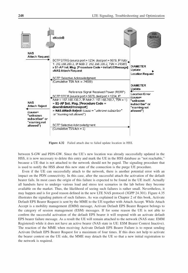
248 LTE Signaling, Troubleshooting and Optimization
Figure 4.32 Failed attach due to failed update location in HSS.
between S-GW and PDN-GW. Since the UE’s new location was already successfully updated in theHSS, it is now necessary to delete this entry and mark the UE in the HSS database as “not reachable,”because a UE that is not attached to the network should not be paged. The signaling procedure thatis used to notify the HSS about this new state of the connection is the purge UE procedure.
Even if the UE can successfully attach to the network, there is another potential error with animpact on the PDN connectivity. In this case, after the successful attach the activation of the defaultbearer fails. In most cases the origin of this failure is expected to be found in the UE itself. Actuallyall handsets have to undergo various load and stress test scenarios in the lab before they becomeavailable on the market. Thus, the likelihood of seeing such failures is rather small. Nevertheless, itmay happen and is for good reason defined in the new LTE NAS protocol (3GPP 24.301). Figure 4.35illustrates the signaling pattern of such failures. As was explained in Chapter 2 of this book, ActivateDefault EPS Bearer Request is sent by the MME to the UE together with Attach Accept. While AttachAccept is a mobility management (EMM) message, Activate Default EPS Bearer Request belongs tothe category of session management (ESM) messages. If for some reason the UE is not able toconfirm the successful activation of the default EPS bearer it will respond with an activate defaultEPS bearer failure message. As a result the UE will remain attached to the network (NAS state: EMMRegistered) while it does not have an active bearer (NAS state in UE: ESM Bearer Context Inactive).The reaction of the MME when receiving Activate Default EPS Bearer Failure is to repeat sendingActivate Default EPS Bearer Request for a maximum of four times. If this does not help to activatethe bearer context on the UE side, the MME may detach the UE so that a new initial registration tothe network is required.

Key Performance Indicators and Measurements for LTE Radio Network Optimization 249
e.g., t = 5s
Figure 4.33 Network failure in attach procedure due to EPC latency.
4.4.1.4 Dedicated Bearer Setup Failure
Whenever a dedicated bearer cannot be established, as shown in Figure 4.36, access to an individualservice and its contents is blocked for the subscriber. With regard to measuring user experience, thiskind of failure should be aggregated on a subscriber ID that can later be used to generate customer-centric reports. However, the aggregation of performance counters for dedicated bearer setup on theservice level (defined by the embedded QoS parameters in the bearer setup request message) and onthe location level (defined by tracking area and E-UTRAN cell ID) is also highly recommended.
The interesting thing about the bearer setup failure is that its message name is “Successful Out-come.” We can see here the same concept that was introduced with the RANAP outcome messagein the UTRAN and also used to confirm successful setup and/or failed setup for a list of multipleRadio Access Bearers (RABs). This is the reason why the message name in S1AP is now “SuccessfulOutcome” even if it reported that the required E-RAB was not going to be established.
The most typical reasons for failed E-RAB setup are drops of the radio connection before RABestablishment is completed. And the eNB may also reject the setup of a particular bearer, becauseit is not able to provide the necessary resources for the requested service, for example, it cannotsupport the desired bit rates. Often the leak of resources is not necessarily related to the availabilityof subcarriers and time slots on the radio interface, but simply to the limited processing power and

250 LTE Signaling, Troubleshooting and Optimization
Figure 4.34 Initial context setup failure during initial attach.
Figure 4.35 Activate Default EPS Bearer Failure.

Key Performance Indicators and Measurements for LTE Radio Network Optimization 251
Figure 4.36 Dedicated bearer setup failure.
the system memory in the eNB. Processors and memory to serve a certain number of connections arefound on so-called “channel cards,” boards that allow scalability of hardware (and in turn scalability ofthe hardware price) according to the amount of expected traffic. If the eNB’s hardware is inadequatethis will result in error messages with cause values like “not enough user plane processing resources,”especially during peak hours of traffic.
4.4.1.5 Paging Failures
The analysis of paging failures requires a distinct workflow rather than just a simple KPI. Due to thetracking area concept of the E-UTRAN, the last known location of a handset that does not respondto paging messages sent by the MME can be more tightly encircled. In a network with one cellrepresenting a single tracking area the UE will be paged in a few cells only, whereas in 2G and 3GRAN paging messages are typically sent to all cells of a particular Location Area Code (LAC) – a fewhundred cells compared to a few dozen in the E-UTRAN. However, a paging failure ratio KPI on cellaggregation level will always have a questionable value due to the fact that a UE can only camp in asingle cell and, hence, from most cells to where the paging was sent there will be no paging response.
It therefore makes sense to store the subscriber ID of UEs that have not answered the paging andinvestigate what may have happened to them before the paging failure and where they may have goneto. The most likely reasons for paging failures are as follows:
• The UE is defective and went out of order without being able to detach from the network.• The UE while in IDLE mode performed a new cell (re)selection and is camping now on a 3G or
2G cell without informing the network properly about the new location that is geographically thesame as before, but covered by a different RAT.
Possible root causes of paging failures to be investigated according to these symptoms are:
• defective handsets;• insufficient coverage;• wrong settings for broadcast cell (re)selection parameters like S0 criteria.
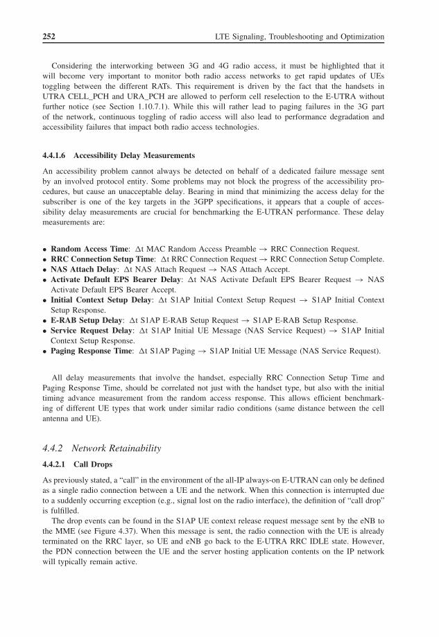
252 LTE Signaling, Troubleshooting and Optimization
Considering the interworking between 3G and 4G radio access, it must be highlighted that itwill become very important to monitor both radio access networks to get rapid updates of UEstoggling between the different RATs. This requirement is driven by the fact that the handsets inUTRA CELL_PCH and URA_PCH are allowed to perform cell reselection to the E-UTRA withoutfurther notice (see Section 1.10.7.1). While this will rather lead to paging failures in the 3G partof the network, continuous toggling of radio access will also lead to performance degradation andaccessibility failures that impact both radio access technologies.
4.4.1.6 Accessibility Delay Measurements
An accessibility problem cannot always be detected on behalf of a dedicated failure message sentby an involved protocol entity. Some problems may not block the progress of the accessibility pro-cedures, but cause an unacceptable delay. Bearing in mind that minimizing the access delay for thesubscriber is one of the key targets in the 3GPP specifications, it appears that a couple of acces-sibility delay measurements are crucial for benchmarking the E-UTRAN performance. These delaymeasurements are:
• Random Access Time: �t MAC Random Access Preamble → RRC Connection Request.• RRC Connection Setup Time: �t RRC Connection Request → RRC Connection Setup Complete.• NAS Attach Delay: �t NAS Attach Request → NAS Attach Accept.• Activate Default EPS Bearer Delay: �t NAS Activate Default EPS Bearer Request → NAS
Activate Default EPS Bearer Accept.• Initial Context Setup Delay: �t S1AP Initial Context Setup Request → S1AP Initial Context
Setup Response.• E-RAB Setup Delay: �t S1AP E-RAB Setup Request → S1AP E-RAB Setup Response.• Service Request Delay: �t S1AP Initial UE Message (NAS Service Request) → S1AP Initial
Context Setup Response.• Paging Response Time: �t S1AP Paging → S1AP Initial UE Message (NAS Service Request).
All delay measurements that involve the handset, especially RRC Connection Setup Time andPaging Response Time, should be correlated not just with the handset type, but also with the initialtiming advance measurement from the random access response. This allows efficient benchmark-ing of different UE types that work under similar radio conditions (same distance between the cellantenna and UE).
4.4.2 Network Retainability
4.4.2.1 Call Drops
As previously stated, a “call” in the environment of the all-IP always-on E-UTRAN can only be definedas a single radio connection between a UE and the network. When this connection is interrupted dueto a suddenly occurring exception (e.g., signal lost on the radio interface), the definition of “call drop”is fulfilled.
The drop events can be found in the S1AP UE context release request message sent by the eNB tothe MME (see Figure 4.37). When this message is sent, the radio connection with the UE is alreadyterminated on the RRC layer, so UE and eNB go back to the E-UTRA RRC IDLE state. However,the PDN connection between the UE and the server hosting application contents on the IP networkwill typically remain active.

Key Performance Indicators and Measurements for LTE Radio Network Optimization 253
Figure 4.37 Call drop due to transmission failures on the radio interface.
The KPI formula for a call drop ratio on the cell aggregation level can be defined as follows:
∑UE Context Release Request (abnormal cause)(∑
S1Ap Initial Context Setup +∑
S1Ap Handover Notify −∑
UE Context Release [cause ′′successful handover′′]) ×100%
(4.8)
In this equation, the total number of active calls is defined as the number of initial contexts suc-cessfully established plus the number of incoming handovers (identified by the S1AP handover notifymessage) minus the number of outgoing handovers (UE Context Release due to “successful handover”).
The “call drop” in the all-IP world of E-UTRAN and EPC will not always be perceived as adropped connection by the subscriber. For non-real-time services like web-browsing or e-mail, userperception is described as rather a temporary interruption of data transport, a delay in accessing thenext web site, or a significant downturn of the data transmission rate of an ongoing download. If thenetwork can re-establish the lost radio connection fast enough (and this is an important KPI for RRCretainability) the drop of the radio connection will not be recognized by the subscriber.
It is a different situation if real-time services are used by the subscriber. In this case the userwill immediately recognize the loss of connection, because the ongoing conversation with the peerparty, for example, in a VoIP call is suddenly interrupted and it would require extremely fast RRCre-establishment procedures (successful re-establishment within 1 or 2 seconds) to save the situation.
Knowing this difference, it appears that it is mandatory not just to compute a call drop ratio percell, but also to have a call drop ratio per service (per QCI is sufficient) within the cell to measurethe user-perceived QoE.
The root causes for call drops are varied and cannot be unambiguously identified just by looking atthe cause value in the S1AP UE context release request message. In fact the identification of the rootcause requires an in-depth analysis of all transport and signaling protocols involved in the call, witha focus on call state transitions and changing radio quality parameters. Figure 4.38 gives an overviewof which different root causes can be revealed from common call drop S1AP causes like “failure inthe radio interface procedure” and “radio connection with UE lost.”
4.4.2.2 RRC Re-Establishment
As discussed in Section 3.2 of this book, it is mandatory for the UE to try a RRC re-establishmentbefore giving up the call as dropped and going back to IDLE. RRC re-establishment can help to
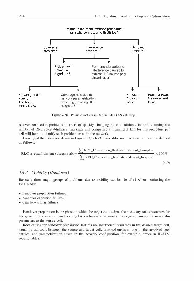
254 LTE Signaling, Troubleshooting and Optimization
Permanent broadbandinterference caused byexternal HF source (e.g.,airport radar)
Coverage hole due tonetwork parametrizationerror, e.g., missing HOneighbor?
Figure 4.38 Possible root causes for an E-UTRAN call drop.
recover connection problems in areas of quickly changing radio conditions. In turn, counting thenumber of RRC re-establishment messages and computing a meaningful KPI for this procedure percell will help to identify such problem areas in the network.
Looking at the messages shown in Figure 3.7, a RRC re-establishment success ratio can be definedas follows:
RRC re-establishment success ratio=∑
RRC_Connection_Re-Establishment_Complete∑RRC_Connection_Re-Establishment_Request
× 100%
(4.9)
4.4.3 Mobility (Handover)
Basically three major groups of problems due to mobility can be identified when monitoring theE-UTRAN:
• handover preparation failures;• handover execution failures;• data forwarding failures.
Handover preparation is the phase in which the target cell assigns the necessary radio resources fortaking over the connection and sending back a handover command message containing the new radioparameters to the source cell.
Root causes for handover preparation failures are insufficient resources in the desired target cell,signaling transport between the source and target cell, protocol errors in one of the involved peerentities, and parametrization errors in the network configuration, for example, errors in IP/ATMrouting tables.

Key Performance Indicators and Measurements for LTE Radio Network Optimization 255
The handover execution phase starts when the previously received handover command message issent to the UE and successfully finished after the UE has arrived at the target cell.
Handover execution can fail because the UE refuses to execute the handover by sending a RRCreconfiguration failure message or if radio contact with the UE is lost during handover execution onthe radio interface.
The various handover procedures in the E-UTRAN can also be classified by their type:
• X2 handover/S1 path switch = Inter-eNB handover with X2.• S1 handover = Inter-eNB handover without X2. Special cases of this scenario are the inter-MME
handover with/without S-GW and/or PDN-GW relocation.• Inter-RAT handover to 3G UTRAN.• Inter-RAT handover to GERAN.• Other inter-RAT handover types, for example, to TD-SCDMA or CDMA2000 radio access tech-
nology (not discussed in more detail in this chapter).• Inter-RAT handover from 3G UTRAN to E-UTRAN.• Inter-RAT handover from GERAN to E-UTRAN.
The handover type can be distinguished according to the interface (X2 or S1) and for S1 accordingto the different containers embedded in the S1AP handover required message. In the case of S1 inter-eNB handover, the Source eNB to Target eNB Transparent Container is included. Inter-RAT handoverto 3G UTRAN requires the Source RNC to Target RNC Transparent Container and inter-RAT handoverto GERAN the Source BSS to Target BSS Transparent Container .
Furthermore, it is necessary to distinguish between incoming and outgoing handover legs in thecase of intra-system S1 handover. This differentiation is possible due to the S1AP mobility elementaryprocedures. While the S1AP handover preparation procedure is found on the outgoing leg, the incomingleg deals with the S1AP handover resource allocation procedure.
4.4.3.1 Handover Preparation
Consequently, the following KPIs can be defined for handover preparation and the failure report shoulddisplay the cause values found in handover failure messages:
X2 handover preparation failure ratio =∑
X2_Handover_Preparation_Failure∑X2_Handover_Request
× 100%
(4.10)
S1 outgoing handover preparation failure ratio =∑
S1AP_Handover_Preparion_Failure∑S1AP_Handover_Required
× 100%
(4.11)1
S1 incoming handover preparation failure ratio =∑
S1AP_Handover_Failure∑S1AP_Handover_Request
× 100% (4.12)
1 Check the embedded container to distinguish between intra-system and inter-RAT handover preparation.

256 LTE Signaling, Troubleshooting and Optimization
The message names used in 3GPP standard documents and in the above KPI formulas need to bemapped to the ASN.1 encoded message format used to construct a particular X2AP/S1AP messagebased on the X2AP/S1AP message type and associated procedure code:
handoverPreparation X2AP-ELEMENTARY-PROCEDURE ::= {
INITIATING MESSAGE HandoverRequest
SUCCESSFUL OUTCOME HandoverRequestAcknowledge
UNSUCCESSFUL OUTCOME HandoverPreparationFailure
PROCEDURE CODE id-handoverPreparation
CRITICALITY reject
}
handoverPreparation S1AP-ELEMENTARY-PROCEDURE ::= {
INITIATING MESSAGE HandoverRequired
SUCCESSFUL OUTCOME HandoverCommand
UNSUCCESSFUL OUTCOME HandoverPreparationFailure
PROCEDURE CODE id-handoverPreparation
CRITICALITY reject
}
handoverResourceAllocation S1AP-ELEMENTARY-PROCEDURE ::= {
INITIATING MESSAGE HandoverRequest
SUCCESSFUL OUTCOME HandoverRequestAcknowledge
UNSUCCESSFUL OUTCOME HandoverFailure
PROCEDURE CODE id-HandoverResourceAllocation
CRITICALITY reject
}
4.4.3.2 Handover Execution
KPIs for the handover execution phase can be defined as follows:
X2 handover execution success ratio =∑
X2_SN_Status_Transfer∑X2_Handover_Request_Acknowledge
× 100% (4.13)
S1 path switch failure ratio =∑
S1AP_Path_Switch_Failure∑S1AP_Path_Switch_Request
× 100% (4.14)
S1 outgoing handover execution success ratio
=∑
S1AP_UE_Context_Release_(′′successful handover′′)∑S1AP_Handover_Command
× 100% (4.15)
The handover type (intra-system or inter-RAT) must be detected according to the previously mon-itored Handover Required message:
S1 incoming handover execution success ratio=∑
S1AP_Handover_Notify∑S1AP_Handover_Request_Acknowledge
×100%
(4.16)

Key Performance Indicators and Measurements for LTE Radio Network Optimization 257
The handover type (intra-system or inter-RAT) must be detected on the source ID found in SourceeNB to Target eNB Transparent Container in the previously monitored handover request message.
One interesting information element is the UE History Information that is included as a mandatoryparameter in the Source eNB to Target eNB Transparent Container and contains a list of up to 6cells maximum visited by the UE before the handover attempt to the target cell. The history caninclude E-UTRAN cells as well as 3G UTRAN cells but is not defined for cells of any other radioaccess technology.
4.4.3.3 Handover Delay Measurements
These measurement are:
• X2 Handover Delay = �t X2AP Handover Request → X2AP Sequence Number (SN) StatusTransfer.
• S1 Path Switch Delay = �t S1AP Path Switch Request → S1AP Path Switch RequestAcknowledge.
• S1 Outgoing Handover Preparation Delay = �t S1AP Handover Required → S1AP HandoverCommand.
• S1 Outgoing Handover Total Delay = �t S1AP Handover Command → S1AP UE ContextRelease (“successful handover”). Although this delay measurement is not meaningful for the userexperience, it is important to measure how long radio resources in the source eNB are blocked aftera handover command was sent to the UE.
• eNB Handover Command Latency = �t S1AP Handover Command → RRC HandoverCommand.
• S1 Incoming Handover Total Delay = �t S1AP Handover Request Acknowledge → S1APHandover Notify.
• eNB Handover Success Latency = �t RRC Handover Confirm → S1AP Handover Notify.
4.4.3.4 Data Forwarding
Data forwarding applies to the X2 handover procedures and can start after the X2AP handover requestacknowledge message is received by the source eNB.
In order to assist the reordering function in the target eNB, the S-GW should send one or more“end marker” packets to the source eNB using the old S1-U path immediately after switching the pathfor each E-RAB of the UE. The “end marker” packets do not contain any user data and are markedwith a special flag in the GTP header. After sending the “end marker” packets, the S-GW should notsend any further user data packets via the old path.
Upon receiving the “end marker” packets from the S-GW via the old S1-U path, the source eNBshould, if forwarding is activated for that bearer, forward the packet toward the target eNB.
The PDCP SN of forwarded Service Data Units (SDUs) is carried in the “PDCP PDU number”field of the GTP-U extension header. The target eNB should use the PDCP SN if it is available in theforwarded GTP-U packet.
Important KPIs for data forwarding are:
• number of forwarded SDUs;• number of lost SDUs;• time difference �t X2AP Handover Request Acknowledge → first UP packet forwarded on X2;• time difference �t first “end marker” packet on old S1-U path → first UP packet forwarded on X2.

258 LTE Signaling, Troubleshooting and Optimization
4.5 User Plane KPIs
User plane KPIs are typically measured on a per call basis. However, this does not mean that theyalways have to be aggregated and stored per call. There are various ways to store and display user planeperformance measurements. Which approach is chosen depends on the purpose of the measurement.What this means will be demonstrated hereafter using the example of throughput measurements.
To get a rough idea of the user plane load it is sufficient to collect the data volume for a longertimer period like 15, 30, or 60 minutes. Based on this time interval, an average throughput can becomputed, but typically this is not done since the data volume fulfills the requirement to have a userplane metric for the busiest cells. However, to describe the user experience in these cells this kind ofmeasurement is not meaningful.
A better way to measure the user experience of throughput is to collect throughput measurementsamples during each call that is active in a particular cell and store and count the results in a binhistogram table. The bin distribution of throughput measurement samples allows a good evaluationof the subscriber’s throughput quality experience. However, the applications used most commonly intoday’s mobile networks are not very throughput sensitive. The throughput graphs in connections thatare mainly used for e-mail and web-browsing services show a profile with high volatility due to thetraffic profile itself. As a result, the distribution of samples in the bin histogram reflects the nature ofthe traffic rather than the experience of the user. Even if the throughput is lower during downloadingelements of, for example, a web site, this is typically not recognized by the subscriber as a problemwith mobile IP access, because the same kinds of issues have been experienced many times before infixed and WLANs for other reasons. Knowing this, it seems that the throughput bin histogram approachis not a universal one. It is meaningful to evaluate the user experience of throughput-sensitive real-time and non-real-time services like streaming video or File Transfer Protocol (FTP), but for a genericmeasurement of user experience and the quality of a cell it does not work. Another disadvantage isthat measuring this kind of throughput requires a lot of hardware. Hence, to deploy it either embeddedin network elements or in using external measurement equipment is very costly and the benefits onegains must be carefully considered versus the expenses.
Another way to gain an impression of the user’s throughput experience is to measure the throughputof a particular connection and store the maximum, minimum, and mean results of this measurementin CDRs. This method works quite well in the lab, where the number of connections and cells to bemonitored is rather small. The use case is to quickly identify under performing calls from a set ofconnections with a known, determined traffic profile.
The most detailed way of throughput measurement presentation is to compute a set of measure-ments that have been sampled at a high sampling rate for the duration of an ongoing connection. Thethroughput measurement results are stored together with their timestamps in a database to be later pre-sented as a table or as a graph along the time axis of a measurement diagram. As shown in Figure 4.39,the highest benefit of this presentation format can be reached if the throughput measurement resultsare shown graphically in correlation with other measurements or with the occurrence of signalingevens (in the figure: handover events) that impact the speed of data transmission. In fact the graphshown in this figure is based on a 3G UTRAN Iub High-Speed Downlink Packet Access (HSDPA)recording, but handover procedures will have the same impact on throughput in 4G E-UTRAN.
In the end it depends on the individual use case what kind of measurement granularity and whichreporting format should or can be chosen. And what was discussed here for throughput measurementsapplies also to most other user plane performance measurements.
4.5.1 IP Throughput
The IP throughput is defined as the data volume of IP frames transmitted within a defined time periodin the UL or DL direction. There are different versions and derivatives of the IP, so a suite of protocolsshould be supported by this measurement, especially as we find in mobile IP networks:

Key Performance Indicators and Measurements for LTE Radio Network Optimization 259
• IPv4 – Internet Protocol version 4 (32-bit addresses).• IPv6 – Internet Protocol version 6 (128-bit addresses).• PIP – The “P”-Internet Protocol.• IP/ST – IP in ST datagram mode.• TP/IX – The “Next” Internet Protocol.• TUBA – Transmission Control Protocol/User Datagram Protocol (TCP/UDP) over Connectionless-
mode Network Protocol (CLNP).
To discuss all the differences between these IP versions is beyond the scope of this book, but theseare surely discussed in various publications about IP services in 3G/4G mobile networks. To readmore about the basic differences between IPv4 and IPv6, refer to Chapter 1 of this book. For thethroughput measurement itself, it does not make a big difference which IP is used. But it is importantthat the protocol frames on the IP layer are correctly decoded.
In the E-UTRAN and EPC there are a couple of different points where the throughput of user planeIP can be measured with different results even within a single call. Most of all, it makes sense tomeasure the IP throughput on the radio interface in order to evaluate the impact on the user experiencein the best possible fashion. Furthermore, it is possible and meaningful to measure IP throughput onthe GTP tunnels of S1-U and S5 and on the SGi. To correlate measurements from the SGi with aparticular mobile subscriber is quite difficult, because there is no tunnel associated with the subscriber.
Dozens of TCP/UDP flows are exchanged between the endpoints (terminal and server) of the IPconnection. To give an example, approximately 30 different IP flows are necessary to download andpresent the complete contents of a typical news web site like www.spiegel-online.de.
While it is easy to detect the sender and receiver of a particular IP packet based on the sourceaddress and destination address in the IP header, it is not so easy to determine which of these addressesbelongs to the subscriber. This knowledge is necessary to enable separate measurements for the ULand DL direction. The best way to sort UL and DL frames is to track the assignment of temporary
Figure 4.39 Throughput measurement graph of a single connection correlated with occurrence of handover events.

260 LTE Signaling, Troubleshooting and Optimization
Figure 4.40 IP frame header.
IP addresses during the attach procedure or to track assignment of GTP tunnel endpoint identifiers inthe tunnel management procedure of GTP-C and S1AP and associate this context information withthe throughput measurements.
The volume of IP data can be easily measured using the length field of the IP header that indicatesthe size of the total IP frame: header plus data. An example is given in Figure 4.40: 1480-byte data +20-byte header = total length of 1500 bytes.
If the total size of the cumulatively counted header length (= data volume!) for a particular calland direction is stored with a 1 second granularity, this value automatically reflects the throughputin bytes per second to be converted into kilobits per second (kbps) or kilobytes per second using asimple post-processing calculation.
4.5.2 Application Throughput
The application throughput for non-real-time services is the data volume measured on the layer 7protocol of TCP/IP user plane protocol stacks divided by time. Basically the measurement approachis the same as explained earlier in the case of IP throughput and the different layer 7 applications canbe distinguished in terms of UDP or TCP port numbers.
There are two challenges for the design of an application that measures application throughput: findout the correct amount of application data volume itself; and find the correct start and stop triggerpoints for the measurement.
To understand the challenge of determining the correct application layer data volume it is useful tolook at an example, namely the FTP frame shown in Figure 4.41.
The FTP frame contains pure data and there is no length field in TCP, just a data offset informationfield. This data offset indicates the first bit of the TCP frame where the payload field of the TCP framebegins. Since the whole TCP frame is organized in multiples of 32 bits (4 bytes) it is clear that 5 ×4 bytes = 20 bytes. This amount needs to be subtracted from the total TCP frame length to get thepayload field size. Now the problem is also that the previous IP frame that carried another TCP blockdoes not contain any information about the TCP payload size, just the total length of the IP frameincluding the header. Often the IP header is 20 bytes long, but we cannot count on this fixed valuebecause, due to a number of options, IP headers may become extremely long – so long that specialalgorithms for IP header compression have been developed.

Key Performance Indicators and Measurements for LTE Radio Network Optimization 261
Figure 4.41 TCP and FTP data frame.
To calculate the FTP data volume using the information available in what is shown in Figure 4.41as the BITMASK column would be easy, but this BITMASK information is delivered by the decoderof the measurement unit, not by the protocol itself, and to refer to this decoder-specific information itneeds a more sophisticated measurement application than one that just adds up values of length fields.For this reason, simple, free-of-charge protocol analysis and measurement software like WireSharkwill most likely never offer application throughput measurements due to the high development efforts.
In the case of UDP it might be a little bit easier, because the UDP header has a fixed size of 8bytes that can be subtracted from the length field that indicates the size of the whole UDP frame: thatis, header plus UDP contents. For an example see Figure 4.42.
Figure 4.42 UDP datagram with length indicator.

262 LTE Signaling, Troubleshooting and Optimization
For real-time services the data volume of Real-Time Transport Protocol (RTP) packets is a goodmetric to determine the throughput, but since there is no length filed in the RTP header, the sizeof RTP blocks must be determined using a little algorithm as is typically implemented in decoderengines. One possible approach is to take the length field from the UDP header if the UDP portsindicate that RTP packets are transported and to plot the length of the payload field (UDP lengthminus UDP header size) in a trailer that comes along with the plain decoder output. By readingthis trailer information and summing the size of RTP blocks over time, it is easy to calculate theRTP throughput.
As already explained, an IP connection consist of multiple TCP and UDP flows that may runsubsequently or in parallel depending on the application. Also, on the IP layer the server addressesare changing depending on the source of contents, for example, a web site. Thus, on the IP layer alsomultiple flows can be identified as shown in the table in upper part of Figure 4.43, which also givesa nice example of data volume and average throughput measurement results in a tabular format thatallows easy detection of the most active IP data flow of this connection.
To see TCP and UDP flows that allow one to distinguish between different application layersaccording to the port numbers, it is necessary to look one layer deeper into the IP flow contents. Hereone can see that UDP immediately transmits application data while TCP needs a startup procedurefor its AM transmissions. This means that the application throughput on UDP can start straight awaywith the application data volume of the first UDP frame that includes the application’s specific UDPport numbers.
In the case of TCP the startup messages of the three-way handshake “syn”–“syn-ack”–“ack” are notused to transmit any application layer data, although they include the port number of the application.Hence, the throughput measurement start trigger should be the first application layer message, forexample, HTTP GET in the case of downloading a web site stream, and the stop trigger for thismeasurement is the HTTP 200OK message.
Figure 4.43 UDP throughput of a connection between two terminal endpoints as measured on S1-U interface.

Key Performance Indicators and Measurements for LTE Radio Network Optimization 263
Last but not least, a strong limitation on measuring the application layer KPIs should be mentioned.In the case of IPsec, which is commonly used for mobile VPN connections, a decoding of TCP/UDPframes is not possible due to the ciphering algorithms used by IPsec. One must bear in mind thatin 3G networks IPsec, at time of writing this chapter (spring 2010), already makes up between30 and 60% of the overall IP data volume transmitted in mobile networks. And this percentage isexpected to rise.
4.5.3 TCP Startup KPIs
For non-real-time services such as file transfer, web-browsing, and e-mail a set of service startupfailure ratio, service startup time, IP service startup failure ratio, and IP service startup time KPIsis defined in ETSI TS 102.250 together with other QoE KPIs such as UL/DL throughput forindividual services.
Originally ETSI TS 102.250 was defined to measure QoS and QoE KPIs with drive test equipment.This explains, for example, the different definitions for service setup time and IP service setup time.The difference is that service setup time refers to start trigger point of the first real application framesent, while IP service setup sees the trigger points for the start and stop of delay measurements in theTCP layer. In fact the service setup time definition also has a fallback to TCP layer-based trigger pointsdefined in case the trigger point cannot be provided from the application layer by the measurementequipment. In the end, service setup and IP service setup trigger points can in fact be identical.
Figure 4.44 shows an example how the (IP) service setup time is measured in the case of FTPservice. It is the time difference for the TCP three-way handshake (see Section 1.10.12). In thisexample the delay between the TCP syn (frame number 1983) and the appropriate first TCP ack(frame number 1992) message is 68 ms. The key for correlating this plain TCP delay measurementwith the application service is to look at the source and destination ports of the TCP header. The portnumbers for the most common non-real-time services currently seen in mobile networks are listedin Table 4.6.
To compute the service startup failure ratio is also quite easy using the same protocol trigger points.Here each TCP syn message is counted as a service attempt and the first ack message of the TCPflow is counted as a success event.
Figure 4.44 FTP (IP) service setup time.

264 LTE Signaling, Troubleshooting and Optimization
Table 4.6 TCP port numbers for common layer 7 applications
TCP port Layer 7 applicationnumber
20, 21 File Transfer Protocol (data and control)80 Hyper Text Transfer Protocol (web-browsing)110 Post Office POP 3 (e-mail)143 Internet Message Access Protocol (e-mail)2848 Wireless Application Protocol (WAP) push MMS
Figure 4.45 TCP round-trip time measurement principle.
4.5.4 TCP Round-Trip Time
The TCP Round-Trip Time (RTT) is the delay between sending a TCP packet identified on behalf ofan individual TCP SN in a particular TCP flow and acknowledgment of this packet in the same TCPflow as shown in Figure 4.45.
When implementing this measurement it must be considered that TCP has some options to workwith selective acknowledgments as defined in RFC 2018. In this case the acknowledgment numberrefers not just to a single sent SN, but to a set of previously sent packets.
The TCP RTT is heavily influenced by radio quality and radio interface procedures. Figure 4.46shows how HARQ retransmissions on the Enhanced Dedicated Channel (E-DCH) of the 3G UTRANtrigger peaks of TCP RTT and how the power control increased the UL SIR (Signal-to-InterferenceRatio) target to prevent further deterioration of user plane QoS. Once increased after the occurrenceof HARQ retransmissions, the UL SIR target is decreased in quick small steps to ensure that theUL interference is kept at a minimum level. Although this figure shows the typical scenarios of a3.5G High-Speed Uplink Packet Access (HSUPA) call, the same power control mechanisms and samecorrelation between retransmission of radio frames and rising RTT can be found in LTE.
4.5.5 Packet Jitter
By definition packet jitter is the average of the deviations from the network mean latency. It is animportant QoS parameter for real-time services using UDP transport due to their delay sensitivity. Fornon-real-time services like web-browsing or e-mail the jitter has no impact on the user plane QoS.

Key Performance Indicators and Measurements for LTE Radio Network Optimization 265
Figure 4.46 HARQ retransmissions cause TCP round-trip time peaks.
The impact of jitter can probably best be understood if a VoIP packet stream is imagined in which aconstant data stream of thousands of small voice packets is expected to be received with high reliabilityand continuity for reassembly and playing back the original audio signal smoothly without any errorthat could be heard by the receiver. Now if the entity that reassembles and transforms the spokenword from the packet stream must wait longer for some individual packets – even if they are receivederror-free – this will cause a delay in the reassembler/transformer that in the worst case can be heardas a gap in the audio signal that comes out of the speaker. Packet jitter is a simple measurement thatallows one to estimate the risk of having the experience of such gaps in the received audio signal.
There are various UDP jitter measurement definitions. The most needed UDP jitter analysis isa “loose” UDP jitter based on the arrival timestamp of subsequently received UDP packets at themeasurement point. For the UDP jitter calculation the formula outlined in Equation 4.17 is used. Inthis formula the individual latency measurement samples for two subsequently received packets of thesame stream are defined as Di and DJ and the difference of these two latency measurement resultsis defined as J (j – i ):
J1 = 0, J2 = (2, 1), Ji = Ji−1 + (|J (i, i − 1)| − Ji−1)
16
∣∣i=3i=∞ (4.17)
The factor 16 that is found in the denominator of Equation 4.17 is a smoothing factor proposed inRFC 1889, the standard specification document for RTP.
4.5.6 Packet Delay and Packet Loss on a Hop-to-Hop Basis
When packet loss or abnormal packet delay is measured at a particular measurement point, the questionwill be raised about which element or part of the network caused such problems. For this kind ofroot cause analysis it is necessary to measure packet loss and packet delay on a hop-to-hop basis, forexample, between Uu and S1-U, between S1-U and S5, and so on.

266 LTE Signaling, Troubleshooting and Optimization
Figure 4.47 Packet delay and lost packet caused by eNodeB.
Figure 4.47 shows the results for the following measurements:
• Packet delay UL: The time the eNB needs to forward a packet received from the Uu to the S1-Uinterface.
• Packet delay DL: The time the eNB needs to forward a packet received from the S1-U interfaceto the Uu interface.
• Lost packets: The total number of lost packets and the time distribution of packet losses accordingto the tracking results after call trace.
The packet delay and packet loss for DL transmissions from S1-U to Uu are shown in the graph; ULdelay measurement results are only displayed in tabular format as a max/min/mean value triple. Notethat the graphs in Figure 4.47 correspond to the UDP throughput shown in Figure 4.43. A comparisonof both figures reveals the loss of packets in eNB as the root cause of the throughput degradationshown in Figure 4.43.