Kolmogorov Spectra Turbulence I - Weizmann Institute of · PDF file ·...
28
VE. Zakharov VS. L'vov G. Falkovich Kolmogorov Spectra of Turbulence I Wave Turbulence ....... 1. Equations of Motion and the Hamiltonian Formalism 1.1 The Hamiltonian Formalism for Waves ................................ in Continuous Media ............ 1.1.1 The Hamiltonian in Normal Variables .... 1.1.2 Interaction Hamiltonian for Weak Nonlinearity 1.1.3 Dynamic Perturbation Theory. .............. Elimination of Nonresonant Terms 1.1.4 Dimensional Analysis .............. .. of the Hamiltonian Coefficients : ........... 1.2 The Hamiltonian Formalism in Hydrodynamics ........ 1.2.1 Clebsh Variables for Ideal Hydrodynamics ........ 1.2.2 Vortex Motion in Incompressible Fluids . : .................... 1.2.3 Sound in Continuous Media 1.2.4 Interaction of Vortex and Potential Motions ........................ in Compressible Fluids ...................... 1.2.5 Waves on Fluid Surfaces ......................... 1.3 Hydrodynamic-Type Systems ....... 1.3.1 Langrnuir and Ion-Sound Waves in Plasma 1.3.2 Atmospheric Rossby Waves and Drift Waves .......... in Inhomogeneous Magnetized Plasmas ........................................ 1.4 Spin Waves 1.4.1 Magnetic Order, Energy and Equations of Motion . . .......................... 1.4.2 Canonical Variables 1.4.3 The Hamiltonian of a Heisenberg Ferromagnet .... 1.4.4 The Hamiltonian of Antifenornagnets ............ ................................... 1.5 Universal Models 1.5.1 Nonlinear Schriidinger Equation for Envelopes .... 1.5.2 Kadomtsev-Petviashvili Equation for Weakly Dispersive Waves .................. .............. 1.5.3 Interaction of Thm Wave Packets 1. Equations of Motion and the Hamiltonian Formalism 1.1 The Hamiltonian Formalism for Waves in Continuous Media Equations describing waves in different media and written in natural variables are diverse. For example, the Bloch equations defining the motion of a mag- netic moment are totally different from the Maxwell equations for nonlinear dielectrics. The latter radically differ from the Euler equations for compressible fluids. However all of them as well as many other equations describing nondis- sipative media, possess an implicit or explicit Hamiltonian structure. This was established empirically and is reflected by the fact that all these models may be derived from initial microscopic Hamiltonian equations of motion. The Hamiltonian method is applicable to a wide class of weakly dissipative wave systems; it clearly manifests general properties of small-amplitude waves. For example, spin, electromagnetic and sound waves are just waves, i.e., medium oscillations, transferred from one point to another. If we are interested only in small-amplitude wave propagation phenomena, such as diffraction, we do not really need to know what it is that oscillates: magnetic moment, electrical field or density. Their respective dispersion law w(k) contains all the information about the medium properties that is necessary and sufficient for studying the propagation of noninteracting waves. As we shall see now, the w(k)-function is a coefficient in the term of the Hamiltonian which is quadratic with respect to wave amplitudes, i.e., to complex normal variables. The actual Hamiltonian is a power series in these variables that contains all the information about nonlinear wave interactions. Let us consider the transition to such variables using a simple yet very important example. 1.1.1 The Hamiltonian in Normal Variables A continuous medium of dimensionality d may be defined in the simplest case by a pair of canonical variables p ( ~ , t) and q ( ~ , t). The canonical equations of motion are expressed as
Transcript of Kolmogorov Spectra Turbulence I - Weizmann Institute of · PDF file ·...

VE. Zakharov VS. L'vov G. Falkovich
Kolmogorov Spectra of Turbulence I Wave Turbulence
....... 1. Equations of Motion and the Hamiltonian Formalism 1.1 The Hamiltonian Formalism for Waves
................................ in Continuous Media ............ 1.1.1 The Hamiltonian in Normal Variables
. . . . 1.1.2 Interaction Hamiltonian for Weak Nonlinearity 1.1.3 Dynamic Perturbation Theory.
.............. Elimination of Nonresonant Terms 1.1.4 Dimensional Analysis
.............. .. of the Hamiltonian Coefficients : ........... 1.2 The Hamiltonian Formalism in Hydrodynamics
........ 1.2.1 Clebsh Variables for Ideal Hydrodynamics
........ 1.2.2 Vortex Motion in Incompressible Fluids . : .................... 1.2.3 Sound in Continuous Media
1.2.4 Interaction of Vortex and Potential Motions ........................ in Compressible Fluids
...................... 1.2.5 Waves on Fluid Surfaces ......................... 1.3 Hydrodynamic-Type Systems
....... 1.3.1 Langrnuir and Ion-Sound Waves in Plasma 1.3.2 Atmospheric Rossby Waves and Drift Waves
.......... in Inhomogeneous Magnetized Plasmas ........................................ 1.4 Spin Waves
1.4.1 Magnetic Order, Energy and Equations of Motion . . .......................... 1.4.2 Canonical Variables
1.4.3 The Hamiltonian of a Heisenberg Ferromagnet .... 1.4.4 The Hamiltonian of Antifenornagnets ............
................................... 1.5 Universal Models 1.5.1 Nonlinear Schriidinger Equation for Envelopes .... 1.5.2 Kadomtsev-Petviashvili Equation
for Weakly Dispersive Waves .................. .............. 1.5.3 Interaction of Thm Wave Packets
1. Equations of Motion and the Hamiltonian Formalism
1.1 The Hamiltonian Formalism for Waves in Continuous Media
Equations describing waves in different media and written in natural variables are diverse. For example, the Bloch equations defining the motion of a mag- netic moment are totally different from the Maxwell equations for nonlinear dielectrics. The latter radically differ from the Euler equations for compressible fluids. However all of them as well as many other equations describing nondis- sipative media, possess an implicit or explicit Hamiltonian structure. This was established empirically and is reflected by the fact that all these models may be derived from initial microscopic Hamiltonian equations of motion.
The Hamiltonian method is applicable to a wide class of weakly dissipative wave systems; it clearly manifests general properties of small-amplitude waves. For example, spin, electromagnetic and sound waves are just waves, i.e., medium oscillations, transferred from one point to another. If we are interested only in small-amplitude wave propagation phenomena, such as diffraction, we do not really need to know what it is that oscillates: magnetic moment, electrical field or density. Their respective dispersion law w(k) contains all the information about the medium properties that is necessary and sufficient for studying the propagation of noninteracting waves. As we shall see now, the w(k)-function is a coefficient in the term of the Hamiltonian which is quadratic with respect to wave amplitudes, i.e., to complex normal variables. The actual Hamiltonian is a power series in these variables that contains all the information about nonlinear wave interactions. Let us consider the transition to such variables using a simple yet very important example.
1.1.1 The Hamiltonian in Normal Variables
A continuous medium of dimensionality d may be defined in the simplest case by a pair of canonical variables p ( ~ , t) and q ( ~ , t). The canonical equations of motion are expressed as
12 1. Equations of Motion and the Hamiltonian Formalism /
1.1 The Hamiltonian Formalism for Waves 13
It is essential that in the new variables a(k) the quadratic part of the Hamiltonian represents a single integral over dk
+B*(k)a*(k, t)a*(-k, t)]) dk ,
In view of (1.1.10), A(k) = A*(k) is a real function and B(k) = B(-k) is an even function. The latter means that we can consider B(k) to be real as well. Indeed, if B(k) = IB(k)lexp[i$(k)], then $(k) = $(-k) and one can dispose of $(k) by substitution a(k) -t a(k)exp[-i+(k)/2]. Let us pose a question: in which case may the Hamiltonian (1.1.15) be diagonalized with respect to the wave vector using a linear transformation
in other words, is there a way to represent it as
First, let us derive the canonicity conditions for this transfopation. On the one hand,
On the other hand, one should require dbldt to equal iSH/Sb* and
Thus, the canonicity conditions take the following form
The parameter u(k) may be chosen to be real without loss in generality, which simply implies a choice of phase for complex variable b(k). Since the value of v(k) may also be chosen to be real [see (1.1.19)l it is convenient to set
According to (1.1.18), ((8) is a real even function. Substituting (1.1.16) into (1.1.15) and comparing to (1.1.17) we obtain after symmetrization with respect to k and -k:
0 = [A(k) + A(-k)]sinh[C(k)lcosh[~(k)l
+ B(k) [cosh2[~(k)l + sinh2[C(k)l] .
Dividing A(k) into even and odd parts
and substituting the respective expressions for B(k), we obtain
for the frequency. Thus, the sign of an even part of w(k) coincides with that of even part of A(k). Expressing cosh[2C(k)] from (1.1.19b) we obtain
w(k) = A2(k) + sign AI ( k ) d ~ i ( k ) - B2(k) . (1.1.20)
One can see that it is only for real w(k) possible to find a diagonalizing transformation. In the variables b(k, t) the equations of motion become trivial
and have the solution b(k,t) = b(k,O)exp[iw(k)t]; thus it is evident that real w(k) implies the stability of the medium against an exponential growth in the wave amplitudes.
In most physical situations, the Hamiltonian is the wave energy density whose sign coincides, by virtue of (1.1.17), with that of the frequency w(k).
In general, wave excitation increases the energy of the medium, which implies that the function w(k) is usually positive. A negative value of w(k) indicates that the energy of the medium decreases with increasing wave excitation. This is possible in systems that are far from thermodynamic equilibrium, for example, in plasmas containing a flux of particles. In that case ak describes the negative- energy waves. It should be borne in mind that the Hamiltonian has been formally defined to an accuracy of a sign, since the transformation H tt -3-1, a tt a* is possible. Therefore the negative-energy waves may be considered only in the case when the w(k) function changes sign in the k-space. What is the connection between a change of sign in w(k) and wave instability? As one can see from
!! 3
5 8
"e
5' <
g z. , =
" iDC
W;
El. a
0
!a 5. . g 8
1 f: I= e
s g
e.
0
PE
3 N
, 5.
0, m
" 5
g g
3 5
a 5
f g.
S .;:
g i;
Ch r
g Y
3
e z 0 3
5.a
0
" 2
.2
zg
* m
g~
g
, e
El.
C) "
C)
8~
8
3 's "g
2.
Y
sg
s
g 5. 6
g 3 5.
a$&
g Ft
. a
XF
; 5.
g Q
'2z
g
aY
s 5-e
e 8 5.
m 3
a
om
3
P.E
. 6's
g. . E. "a
16 1. Equations of Motion and the Hamiltonian Formalism 1.1 The Hamiltonian Formalism for Waves 17
with p = (kl k2k3 k4) . (1.1.24b)
The coefficients of the interaction Hamiltonian have the following obvious properties
V(k1, k2, k3) = V(kl, k3, k2),
U(k1, k2, k3) = U(ki, ks, k2) = U(k2, k i , 631,
G(k1, k2, k3, k4) = G(k1, k3, k2,k4) = G(ki,k2,k4,hs),
W(k1, k2, k3, k4) = W(k2,k1, k3, k4) (1.1.25)
= W(k1, k2, k4,k3) = W*(k3, k4, ki, k2),
R(k1, k2, ks, k3) = R(k2, ki , k3, k4) = R(ki, k2, k4, k3)
= R(k3, E2, kl , k4) = R(k4,k2, k3, ki) . The last equation for W(kl, k2, k3, k4) follows since the Hamiltonian is real.
But to which order in b, b* should we expand the Harniltonian 'FI? The answer turns out to be as general as the question: "?is and higher-order terms should normally not be taken into account" This can be explained as follows: Since the expansion uses a small parameter, every subsequent term is smaller than the preceding one, and the dynamics of the wave system is determined by the very first term of 'Hint, i.e., normally X3. However, three-wave processes may turn out to be "nonresonant" which means that the spatio-temporal synchronization condition (or, in terms of quasi-particles, the momentum-energy conservation law)
cannot be satisfied. Let d be the dimensionality of the medium and k the vector in d-meric space (d > 1). Equation (1.1.26) specifies the hypersurface of dimension 2d - 1 in the 2d-meric space of vectors k, kl. If this surface does in fact exist [i.e., w(k) is real], the dispersion law w(k) is of the decay type. If (1.1.26) has no real solutions, the dispersion law is of the nondecay type.
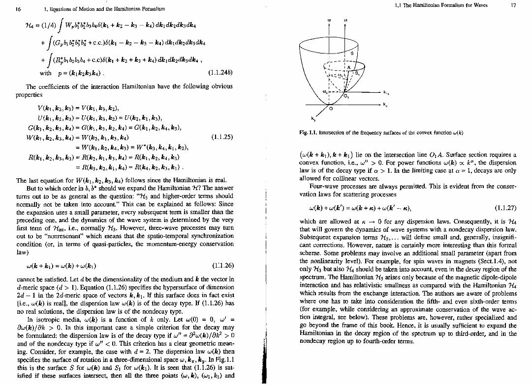
In isotropic media, w(k) is a function of k only. Let w(0) = 0, w' = dw(k)/dk > 0. In this important case a simple criterion for the decay may be formulated: the dispersion law is of the decay type if w" = d2w(k)/dk2 > 0 and of the nondecay type if w" < 0. This criterion has a clear geometric mean- ing. Consider, for example, the case with d = 2. The dispersion law w(k) then specifies the surface of rotation in a three-dimensional space w, k,, k,. In Fig.l.1 this is the surface S for w(h) and Sl for w(k1). It is seen that (1.1.26) is sat- isfied if these surfaces intersect, then all the three points (w, k), (wl, k1) and
Fig. 1.1. Intersection of the frequency surfaces of the convex function w(k)
(w(k + kl), k + kl ) lie on the intersection line O1 A. Surface section requires a convex function, i.e., w" > 0. For power functions w(k) ar ka, the dispersion law is of the decay type if a > 1. In the limiting case at a = 1, decays are only allowed for collinear vectors.
Four-wave processes are always permitted. This is evident from the conser- vation laws for scattering processes
which are allowed at rc. -t 0 for any dispersion laws. Consequently, it is 'H4
that will govern the dynamics of wave systems with a nondecay dispersion law. Subsequent expansion terms 'F15,. . . will define small and, generally, insignifi- cant corrections. However, nature is certainly more interesting than this formal scheme. Some problems may involve an additional small parameter (apart from the nonlinearity level). For example, for spin waves in magnets (Sect.l.4), not only 'Id3 but also 'I& should be taken into account, even in the decay region of the spectrum. The Hamiltonian 'F13 arises only because of the magnetic dipole-dipole interaction and has relativistic smallness as compared with the Hamiltonian 'Id4 which results from the exchange interaction. The authors are aware of problems where one has to take into consideration the fifth- and even sixth-order terms (for example, while considering an approximate conservation of the wave ac- tion integral, see below). These problems are, however, rather specialized and go beyond the frame of this book. Hence, it is usually sufficient to expand the Hamiltonian in the decay region of the spectrum up to third-order, and in the nondecay region up to fourth-order terms.
18 1. Equations of Motion and the Hamiltonian Formalism
I
I 1.1 The Hamiltonian Formalism for Waves 19
1.1.3 Dynamic Perturbation Theory. Elimination of Nonresonant Terms
It is intuitively clear that in the case of a nondecay dispersion law, the Hamilto- nian 3-1.3 describing three-wave processes may turn out to be irfelevant in some respect. We shall show now that in this case one can go over to new canon- ical "ariables ck,c;, such that 113{ck,c~} = 0. This is possible because the dynamic system under consideration, the weakly nonlinear wave field, is close to a completely integrable dynamic system (a set of noninteracting oscillators). Traditionally classical perturbation theory is employed to handle systems close to completely integrable ones. In this procedure a canonical transformation is derived by sequentially excluding the nonintegrable terms from the Hamiltonian. It is known that the procedure may encounter the problem of "small resonance denominators"; then the only terms to be excluded from the Harniltonian are those for which the resonance condition is not satisfied. As shown by Zakharov [1.1], we can in this case to some extent apply classical perturbation theory.
Let us demonstrate such a procedure using a simple example. Consider the expansion of the one-wave Hamiltonian:
v U 'FI= %+'?dj +'h$ = wbb* +-(b2b* + b*2b)+ -(b3 + b*3) 2 6
We assume every subsequent term to be smaller than the preceding one, i.e. 'Flz >> U3 >> U4. Since one needs to eliminate the ?-L3 term without changing 3-12, the transformation must be close to the unity trarisformation. Thus it is reasonable to search for the transformation in the form of an expansion, which starts from a linear term:
Why do we take the following (c3-order) terms into account? Taking only the lin- ear and quadratic terms in (1.1.28a) into account is indeed sufficient to eliminate the U3 term. In that case the fourth-order terms govern the nonlinear interaction. Due to the transformation they will acquire additional terms. To derive these new terms 2-order terms in (1.1.28a) have to be taken into account. Moreover, we will use them to exclude the last two terms describing the 1 + 3 and 0 -+ 4 processes in the Hamiltonian (1.1.24b).
Thus we look for seven coefficients: A1, A2, A3, B1, . . . , B4. The canonicity condition (1.1.7) is expressed through the Poisson brackets and has the form
db db* db* db {bb*) = -- - -- = 1. ac ace ac ace Computing the Poisson bracket to an accuracy of 2-order terms, we obtain three equations
Substituting (1.1.28a) into the Hamiltonian and demanding that all nonlinear terms (except c?c*~) vanish, we have four equations
From these it is easy to find the transformation coefficients
In the new variables the Hamiltonian has the simple form
It is easily seen that neglect of the cubic terms in (1.1.28a), would have given wrong values of the additional interaction coefficients supplementing W.
Following the same pattern, let us return to the general case and use a trans- formation in the form of a power series to eliminate cubic and nonresonant fourth-order terms. In the new variables the Hamiltonian of interaction describes 2 -+ 2 processes (for details see Sect. A.3):
Here (J' f i) = kj f k;. Note that (1.1.29b) is true on the resonant surface
1.1 The Hamiltonian Formalism for Waves 21 20 1. Equations of Motion and the Hamiltonian Formalism
only, where the coefficient TL has the same properties (1.1.25) as W,. The necessity of taking cubic terms into account for the transformation to yield the correct value of the four-wave interaction coefficient was first pointed out by Krasitskii [ 1.21.
Let us discuss the singularities of (1.1.29). The denominators become zero on the resonance surfaces of three-wave processes:
and
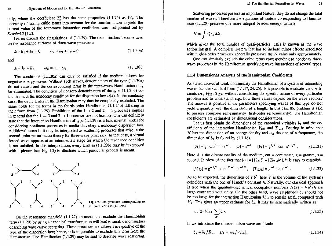
The conditions (1.1.30a) can only be satisfied if the medium allows for negative-energy waves. Without such waves, denominators of the type (1.1.30a) do not vanish and the corresponding terms in the three-wave Hamiltonian may be eliminated. The condition of nonzero denominators of the type (1.1.30b) co- incides with the nondecay condition for the dispersion law w(k). In the nondecay case, the cubic terms in the Hamiltonian may thus be completely excluded. The same holds for the terms in the fourth-order Hamiltonian (1.1.24b) differing in their form from (1.1.29). Prohibition of the 1 4 2 and 2 t 1 processes implies in general that the 1 t 3 and 3 t 1 processes are not feasible. One can definitely state that the interaction Harniltonian of type (1.1.29) is a fundamental model for considering nonlinear processes in media that obey a nondecay dispersion law. Additional terms in it may be interpreted as scattering processes that arise in the second order perturbation theory for three-wave processes. In that case, a virtual forced wave appears at an intermediate stage for which the resonance condition is not satisfied. In this interpretation, every term in (1.1.29b) may be juxtaposed with a picture (see Fig. 1.2) to illustrate which particular process is meant.
3
1 2 4 2 1 4 '1 2 4 '1 2 4 Fig. different 1.2. The terms processes in (l.l.29b) corresponding to
On the resonance manifold (1.1.27) an attempt to exclude the Hamiltonian term (1.1.29) by using a canonical transformation will lead to small denominators describing wave-wave scattering. These processes are allowed irrespective of the type of the dispersion law; hence, it is impossible to exclude this term from the Hamiltonian. The Hamiltonian (1.1.29) may be said to describe wave scattering.
Scattering processes possess an important feature: they do not change the total number of waves. Therefore the equations of motion corresponding to Hamilto- nian (1.1.29) preserve one more integral besides energy, namely
which gives the total number of quasi-particles. This is known as the wave action integral. A complete system that has to include minor effects associated with higher-order processes generally preserves the N value only approximately.
One can similarly exclude the cubic terms corresponding to nondecay three- wave processes in the Harniltonian specifying wave interactions of several types.
1.1.4 Dimensional Analysis of the Hamiltonian Coefficients
As stated above, at weak nonlinearity the Hamiltonian of a system of interacting waves has the standard form (1.1.17,24,25). Is it possible to evaluate the coeffi- cients wk, V123, T l 2 ~ without considering the specific nature of every pdcular problem and to understand, e.g., how these values depend on the wave vectors? The answer is positive if the parameters specifying waves of this type do not yield a quantity with the dimension of a length. In this case the problem is said to possess complete self-similarity (first-order self-similarity). The Hamiltonian coefficients are estimated by dimensional considerations.
Let us first obtain the dimensions of the canonical variables bk and the co- efficients of the interaction Hamiltonian VI23 and T1234. Bearing in mind that Ft has the dimension of an energy density and wk the one of a frequency, the dimension of bk is found by (1.1.18).
Here d is the dimensionality of the medium, cm = centimeter, g = gramm, s = second. In view of the fact that [w] = [ 6 2 3 b ] = [ T ~ ~ M ~ ~ ] , it is easy to establish
As to be expected, the dimension of vb2 (here V is the volume of the system!) coincides with the one of Planck's constant ti. Naturally, our classical approach is true when the quantum-mechanical occupation numbers N(k) = vb2/h are large compared with unity. On the other hand, wave amplitudes bk should not be too large for the interaction Hamiltonian 'Hint to remain small compared with 7-h. This gives an upper estimate for bk. It may be schematically written as
If we introduce the dimensionless wave amplitude
22 1. Equations of Motion and the Hamiltonian Formalism 1.1 The Hamiltonian Formalism for Waves 23
the weak nonlinearity condition may be written as
Now we can discuss some particular examples.
Sound in Continuous Media. As parameters the equations of motion for this problem may include only the medium's density Q and the elasticity coefficient IE with the respective dimensions [el = g . and [IE] = g cm-I - sb2. These values and the wave vector k combine to yield the dimension of a frequency [w] = s-' = [eznYkr] = gz+y . ~ m - ~ ' - y + ~ - s - ~ Y . Equating the exponents at g, cm and s, we have three equations x + y = 0, 3x + y + z = 0, and 2y = 1. Hence x = -112, y = 112, z = 1. Thus the dimensional analysis leads to a linear law for the wave dispersion
Here c, is the sound velocity and a a dimensionless parameter of the order of unity. From the parameters of our problem, one can also obtain Bk with the dimension of the canonical variable bk
and the interaction coefficient
Here the dimensionless function f depends on eight dimensionless arguments: the two ratios k2/kl and k3/kl, and six angle variables giving the directions of the three vectors. In fact, there are only three angle variables: cos 812, cos 813, and cos 023 [here cos eij = (kikj)/kikj], as our system has no preferred direction.
In the Hamiltonian description, the wave amplitude is proportional to bk. In the sound wave field, medium density p(r, t) = @ + el (r, t ) and velocity oscillate:
where pk, vk are the respective wave amplitudes in natural variables. In the linear approximation the relationship between natural and normal canonical variables is easily established from dimensional considerations
The symbol "cx" designates proportionality. In terms of canonical variables the condition of weak nonlinearity is written as
The symbol ''N" denotes an estimate to an accuracy of a dimensionless factor of order unity.
Gravitational Waves on a Fluid Surface. These are relatively long waves for which surface tension is insignificant and the force tending to restore the equi- librium state of the surface is the gravitational force. Apart from fluid density Q
the significant parameters should evidently include the gravitational acceleration g, [g] = cm r2. Following the scheme given in the preceding example and bearing in mind that this is a 2-dimensional problem (d = 2), we have:
As we see, the dispersion law is of the nondecay type, wk cx ka , a = 112 < 1. Therefore the principal interaction is four-wave, with the interaction coefficient
A natural variable describing water waves is q(r), the deviation of the fluid surface from the unperturbed state and the dimensionless wave amplitude is E k = kqk = bk/Bk. Whence, we obtain
Capillary Waves. For sufficiently short waves the restoring force should be entirely determined by surface tension. The significant parameters should in this case instead of g include the surface tension coefficient u having the dimension of a surface energy [a] = g - s - ~ . Thus,
The dispersion law of capillary waves is of the decay type: a = 312 > 1. Therefore the three-wave interaction remains as the most essential one
Comparing the dispersion laws of capillary (1.1.45) and gravitational waves (1.1.42), it is easy to find the boundary value of the wave vector at which these frequencies coincide:
24 1. Equations of Motion and the Hamiltonian Formalism 1.2 The Hamiltonian Formalism in Hydrodynamics 25
At k << k,, the gravitational energy of a wave is larger than the surface tension energy and the latter may be neglected. Thus long waves on a fluid surface will be gravitational. Accordingly, at k >> k, the surface waves will be capillary with the dispersion law (1.1.45). We shall show in Sect. 1.2 below that at arbitrary k's the dispersion law for waves on the surface of a deep fluid is expressed as
Though dimensional estimates usually give answers to the accuracy of a dimen- sionless factor of the order of unity, the dispersion laws (1.1.42,45) are accurate in the limits of large and small wavelength, respectively.
For water waves at room temperature, k, N 4 cm (Q = lg/cm3, a = 70g/s2). This corresponds to a wavelength of X = 2n/k, 2 1.6 cm and frequency f, = w*/2n E 0.2 Hz.
Vortex Motions of Incompressible Fluids. From the viewpoint of dimensional analysis, this problem radically differs from the preceding problems in that it has only one significant parameter, the fluid density [&I = g/cm3. Still, this allows to determine the Hamiltonian structure. In particular, since it is impossible to build from p~ and k a combination with the dimension of a frequency, it should not contain an 'Hz = Jwka;ak dk term, i.e., 'H2 = 0. Using (1.1.31-32), one can easily see that among all factors of the 'H-expansion into a power series, only the coefficient at a4 has a dimension containing no time. Therefore, only this factor may be derived from p~ and k:
It immediately follows that the nonlinearity of incompressible fluid motion is extremely strong, ( = + CCI. Another important consequence of di- mensional analysis is the nonlinear relationship between fluid velocity vk and canonical variables ak. If we formally represent vk as a power series of ak::
the dimension of a single coefficient & will contain no time. From this, 4, = 43 = . . . = 0, 4 2 = k/&. Therefore
It is now clear why the Hamiltonian of the problem 'H = (112) j lv(r)I2 dr is proportional to the fourth power of the canonical variables ak, a;.
This section has given the general structure of canonical equations of motion for weakly nonlinear waves. The remaining sections of this chapter deal with various specific systems, the introduction of canonical variables and calculation of Hamiltonian coefficients. Readers who are not interested in the character of
waves in different media and the technique for deriving the canonical equations may go over directly to Chap.2 where the kinetic wave equation is obtained from the dynamic equations given in Sect. 1.1. The paragraphs left out in the first reading, may then be referred to when evaluating the coefficients of the Hamiltonian.
1.2 The Hamiltonian Formalism in Hydrodynamics
The ideal incompressible fluid is the simplest and most important representative of a wide class of dynamic systems of the hydrodynamic type and is thus widely used in physical problems. For zero dissipation all these systems possess an im- plicit Hamiltonian structure. The description of such structures and the related group-theoretical formulations constitute a formidable mathematical problem ex- tending far beyond the scope of this book (those interested in it are referred to [1.3]). For our purposes it will be sufficient to discuss the introduction of canon- ical variables only for several cases that are most important for the turbulence theory. Appropriate canonical variables for an imcompressible fluid were first presented by Clebsh (see [1.4]) in the last century. Independently Bateman [1.5] and later on Davydov [1.6] gave the canonical variables for barotropic flows in incompressible fluids with single-valued functions for the pressure. These results will be discussed in Sect. 1.2.1. Further on we shall obtain the Hamiltonians for vortex motion 'Hv (Sect. 1.2.2), for small-amplitude (potential) motion of sound 'Hs (Sect. 1.2.3) and for sound-vortex interactions 'Hsv(Sect. 1.2.4). Fluid strat- ification gives rise to new types of motions localized in the regions of maximal inhomogenities. In the extremely nonuniform case of the free surface of a fluid, these are the known surface waves. The canonical variables for them were ob- tained by Zakharov [1.7]. For the general case with arbitrary wavelength and fluid depth the Hamiltonian description of this type of motion will be given in Sects. 1.2.5,6.
1.2.1 CIebsh Variables for Ideal Hydrodynamics
Consider the Euler equations for compressible fluids:
a@/& + div ev = 0 , (1.2.1~)
Here v(r, t) is the Eulerian fluid velocity (in the point T at the moment of time t ) ; e(r, t) the density and p(r, t) is the pressure which, in the general case, is a function of fluid density and specific entropy s, i.e., p = p(p, s). In ideal fluids where there is neither viscosity nor heat exchange, the entropy per unit volume is carried by the fluid, i.e., it obeys as/& + (vV)s = 0. A fluid in which the specific entropy is constant throughout the volume is called barotropic. In such a fluid the pressure is a single-valued function of the density p = p ( ~ ) . In this

26 1. Equations of Motion and the Hamiltonian Formalism 1.2 The Hamiltonian Formalism in Hydrodynamics 27
case, Vp/e may be expressed via the gradient of the specific enthalpy of the unit mass w = E + P V and dw = VdP = dP/e. Thus, Vp/p = Vw. The enthalpy in turn equals the derivative of the internal energy of the unit volume E(Q) = EQ with respect to the fluid density
Direct differentiation with respect to time shows that (1.2.1) conserves the full energy of the fluid
In line with Thomson's theorem, these equations also conserve the velocity cir- culation around a "fluid" path. This means that there exists a scalar function p(r, t) which moves together with the fluid:
In our search for the canonical variables for the Euler equations (1.2.1), we shall use the Lagrangian approach. For that purpose, we shall consider the known expression for the Lagrangian of a mechanical system (kinetic minus potential energy), generalized for the continuous case and use as external constraints the continuity equation (1.2.la) and Thomson's theorem (1.2.3):
@ and A are the undetermined Lagrange multipliers. Variation with respect to them leads to (1.2.la) and (1.2.3). A single integration by parts allows to rewrite the Lagrangian (1.2.4) as
ae a p v2 L {cp- -A-+@--
J a t at 2
Consider the action S = S L dt. Due to its extremality, the condition SS/Sv = 0 should be satisfied, which is equivalent to the condition S L / h = 0. From (1.2.5), we have
As the Lagrangian (1.2.5) and (1.2.6) do not contain time derivatives we can substitute (1.2.6) into (1.2.5) to arrive at the Lagrangian of the Hamiltonian system,
for which the pairs (Q, @) and (A, p) are pairs of canonically-conjugate variables. Using (1.2.2) and (1.2.6) it is easy to compute the variational derivatives with respect to e and A,
[a , b] = a x b denotes the vector product. In calculating the derivatives with respect to @ and p, one has to integrate by parts.
Thus (1.2.9) and (1.2.10) have the forms
dX/at + div Xv = 0 .
As to be expected (1.2.8) and (1.2.11) coincide with the continuity equations (1.2. la) and (1.2.3), respectively.
Let us consider now to what extent the system of equations (1.2.8-11) is equivalent to the initial hydrodynamic system for the three components of ve- locity and density. The solvability of (1.2.8-11) should imply that (1.2.1) are satisfied for the velocity given by (1.2.6). This may be verified by direct calcula- tion of the av/& derivative. The question of reverse correspondence reduces to the following one: can we always represent the velocity field V(T, t) in the form of (1.2.6)? To answer this question, we calculate the vorticity. From (1.2.6), we have
rotv = [V(X/e), Vp] = [Vd, Vp], 19 = A / @ . (1.2.12)
Evidently, div [Vd, Vp] = 0. Now we introduce the q, = (v rot v) value, the helicity density of the velocity field. From (1.2.6) and (1.2.16). we have
9s = (v[Vd, Vpl) = (V@[V6, Vp]) = div O[Vd, Vp] . (1.2.13)
28 1. Equations of Motion and the Hamiltonian Formalism 1.2 The Hamiltoninn Fomaliim in Hydrodynamics 29
The Q, = J q, dr value is called the helicity of the velocity field and represents an integral of motion of the hydrodynamic equations. From (1.2.13) it is seen that the possibility of representing the velocity as (1.2.6) means that Q, = 0. As a matter of fact, it is easy to construct examples of the velocity fields for which Q, +O. Let, e.g., v satisfy of the system of equations (a =const)
rot v = a v , div v = 0 (Beltramy flow) .
It should be noted that the fields obeying these equations are the stationary solu- tions of the hydrodynamic equations with the density p =const. It is easily seen that for such flows Q, = a J v2 dr # 0. The condition allowing to represent the velocity field as (1.2.6) may be interpreted geometrically. According to the logic of our construction, p(r) and 6 ( ~ ) are single-valued functions of the coordinates. It follows from (1.2.12) that the vector rot v is directed along the intersection line of the level surfaces of these functions. Not every closed line may be represented as an intersection line of level surfaces of single-valued functions. This is, for example, not feasible if the line is knotted, i.e., if it represents the circle image unhomotopic to it. Let such a line be specified by the equation r = l(y) where y is a parameter on the line, and the vorticity field is expressed as (the vortex line)
rot v = K n(y)6[~ - l(y)ldy, JnI2 = 1 . I Topology manuals (see also [1.8]) prove that in this case Q, = mK2 where
m is an integer defining the winding number (knotticity) of the line. A similar formula holds if the line represents a pair of linked circles with m = 1.
We shall refer to the variables p, @, X and p as the Clebsch variables. Evi- dently, a global definition of the Clebsch variables is not always possible, as it requires zero knotticity of the vortex lines. At least in the vicinity of a regular point of the velocity field, the local introduction of the Clebsch variables is al- ways possible, but attempts to expand the range of validity of their functions may lead to a loss of the single-valuedness of X and 9. Nevertheless, it is possible to introduce several pairs of Clebsch variables (Xi, pi), i = 1,. . . N:
api/dt + (vV)pi = 0, dXi/dt + div (XV) = O ,
Probably, one can prove that N = 2 is sufficient to establish a one-to-one equiva- lence between the initial hydrodynamic system and a canonical one for arbitrary flows.
1.2.2 Vortex Motion in Incompressible Fluids
In the case of an incompressible fluid with dp/% = 0, we can set .g = 1 (to simplify the notation). The velocity may now be written as v = XVp + V9. The condition div v = 0 yields @ : @ = -A-'div XVp. The formula for the velocity may be rewritten as
Here A-' is the inverse operator to the Laplacian. Hence, we have now only one pair of the Clebsch variables A, p. Fourier transformation and the transition to complex variables
allow to cast the canonical equations (1.2.10-1 1) into the standard form (1.1.6):
da(k, t)/dt = 6'FIv/6a*(k, t).
The Hamiltonian 'FIv is obtained by substituting the formula for the velocity into the expression for the kinetic energy (1.2.2)
Here
which follows from (1.2.14). As a result, we have
Hv = $ / ~12,34a~c$a3~46(kl + k2 - k3 - k4) d l l dk2dk3dk4 , (1.2.16~)
where the interaction coefficient is
The expressions (1.2.1$,16) agree with the dimensional estimates (1.1.49-50) obtained in Sect. 1.1.5.
1.2.3 Sound in Continuous Media
As seen from (1.2.6), the case with X = 0 or p =const corresponds to poten- tial fluid motion which is according to (1.2.8-9) defined by a pair of variables (.g,@). Following the standard scheme presented in Sect. 1.1, we go in the k- representation from the real canonical variables @(k), p(k) over to the complex b(k), b*(k):
30 1. Equations of Motion and the Hamiltonian Formalism 1.2 The Hamiltonian Formalism in Hydrodynamics 31
b ~ ( k ) = k(p~ /bk ) ' /~ [b (k ) + b*(-k)] , (1.2.17a) I
(1.2.17b) ~ ( k ) = kc,, 4 = (aplae) . I
Here Se = e - eo is density deviation fiom the steady state and c, the sound velocity. The derivative (aplae) is calculated with the entropy s treated as a ! constant, which corresponds to assuming a barotropic motion of the fluid (without heat exchange). Equations (1.2.17) coincide to an accuracy of a dimensionless multiplier of the order of unity with the dimensional estimates (1.1.36) and i (1.1.40). In order to obtain the sound Hamiltonian Ns one should expand the I
expression for energy (1.2.2) in terms of 6e and v = V@ 1
NSS = / [6elv@12 + gci(6e)'l d~ , and substitute Qi and Sp from (1.2.17) into these expressions. As a result, we see i
that the quadratic part of the Harniltonian is diagonal in the variables bk, 6;. i i
The Harniltonian of the sound-sound interaction Nss has the form (1.1.24a) with the interaction coefficients:
V(k, kt, k2) = U(k, k1, k2) 112 (1.2.20)
(39 + cos + cos dk2 + cos 612) .
As expected, this expression is consistent with the result (1.1.38) obtained from a dimensional analysis by specifying the type of angular dependence f.
The supposition that the density of the internal energy E(T) depends only on @(T) is true only in the range of small inhomogeneities. In the general case, the internal energy Ei, is a density functional which may be represented as a power series in Ve:
Whence, the expression for the frequency w(k) will change from (1.2.17b) to I
It should be noted, that /? may be either positive or negative [see, e.g., (1.2.39,41) and (1.3.10)l. The expression (1.2.22) is true if the dispersion of sound is small: /?k2 -K 24. Otherwise, one should take into account the next Ve-terms.
1.2.4 Interaction of Vortex and Potential Motions in Compressible Fluids
As shown above, in incompressible fluids, the variables X and p define vortex motion. A purely potential motion is described by the pair Q and Qi. However, in the general case it is wrong to assert that this pair e and @ describes potential motion and X and p vortex motion. Indeed, dividing v into two parts
v = v1 + v2, rot v1 = 0, div v2 = 0 ,
we see that
Therefore the initial Clebsh variables are inconvenient for describing the turbu- lence of compressible fluids: the fields (e, I) and (A, p ) are strongly coupled; even for small fluctuation velocity (with the Mach number M)
Formally this manifests itself in the fact that the coefficient of interaction between these fields increases with the sound velocity rn A.
Assuming the Mach number M to be small, L'jov and Mikhailov obtain a canonical transformation separating potential and vortex motions in the new variables (q, p) and (Q, P) [1.9]. In doing so we shall try to determine the vor- tex velocity v2 and the potential velocity vl by equations close to (1.2.12) and (1.2.23), respectively. We choose the desired canonical transformation using the generating functional F depending on the new coordinates q, Q and the old momenta 9, p (see (A.2.12) in Sect. A.2)
We write the generating functional as
where Fo is a functional of the identity transformation chosen in such a way that the pair of canonical variables responsible for potential motion is q = p and p = 6. The functional 4 is independent of 4, bilinear in p and Q and represents a power series of the variable part of density 6e = e(r, t) - po:
The expansion parameter is

! 1.2 The Hamiltonian Formalism in Hydrodynamics 33 32 1. Equations of Motion and the Hamiltonian Formalism
where ks E l / X s and kv = 1/L are the characteristic wave vectors of sound waves and vortices, respectively; Es is the energy of sound motions.
Substituting (1.2.25~) and (1.2.25d) in (1.2.25a) and solving the resulting equations by iterations with regard to the small parameter J << 1, we obtain
Here nj = kj/k, and pi j are determined by (1.2.15b). The term Xsvl de- scribes sound scattering processes and the 'FIsv2-term describes generation and absorption of sound by turbulence. In (1.2.29a) we have not written out the terms S(")a*u 1 2 bn+2, ~ ( ~ ) a ~ a * ~ b ~ + ' , n 2 1, which are small in the Jn parameter and insignificant for our future considerations.
= Q + (V, ~ - ' v ~ e ) Q l e o + 0(J2) , p = P + (VP, A - ' V S Q ) / ~ + 0( t2) . 1.2.5 Waves on Fluid Surfaces
In the new variables Let us consider potential motion of incompressible fluids with a free surface in
I a homogeneous gravitational fluid [1.7]. In the quiescent state the fluid surface is a plane z = 0 with the bottom at z = -h. We describe the surface form by
= ~ ( r , t) where r = (x, y) is the coordinate in the transverse plane. The full
I energy of the fluid 'FI = T + 17 is a sum of the kinetic energy
v2 = [VQ, VPI (1.2.27b)
- [V, [V, [A-' ve, [VP, VQI I I I + 0(J2) . Thus we achieved the desired result: the potential motions are defined by the
pair (q, p) only; the main contribution to vortex motion is made by the pair Q, P. The last term in (1.2.27b) for v2 describes the effect of compressibility on the vortex motion.
In the k-representation, we go over to the complex variables b(k), b*(k), and a(k), a*(k) following formulas similar to (1.2.17) and (1.1.3-4). In these variables the hydrodynamic equations have the canonical form
I and the potential energy
Here g is the gravitational acceleration; cr the surface tension coefficient and the free surface element is expressed by ds = d r d m .
I In constructing the canonical variables we shall proceed from the Hamiltonian ~ (1.2.7) where we set
with the Hamiltonian
Here O(6) = 1 at [ > 0, O(E) = 0 at [ < 0. Further on we shall consider I only irrotational fluid flows implying that may use X = 0. Substituting (1.2.31)
into (1.2.7) and taking advantage of the fact that aq(r,z,t)/& = S[q(r,t) - 1 z ] d ~ ( r , t)/at, the Lagrangian reads
The sound Hamiltonian has the form (1.2.18), the Hamiltonian of vortex motions is specified by (1.2.16), and the Hamiltonian of sound-vortex interaction has two terms:
Here P(T, t) = @(T, Z, t) at z = q(r , t). The Lagrangian (1.2.32) yields the canonical equations

34 1. Equations of Motion and the Hamiltonian Formalism
Thus the canonical pair of variables is now given by q(r,t), 9(r , t ) . Having specified them, we have now to solve the boundary value problem for the Laplace equation
in order to determine the fluid's velocity field. Now v = V 9 and we get
for the kinetic energy. The variation 6'H/S9 = ST/69 may be carried out explic- itly, but the result is known in advance. To obtain it, we substitute e = O(q - z) into the continuity equation (1.2.1) to get
as the kinematic condition on the fluid surface which should coincide with (1.2.33a). The physical meaning of this condition is rather simple: the veloc- ity of fluid height-variations should be the same as the velocity of the fluid itself in the given point at the surface.
The explicit solution of the boundary value problem (1.2.34) is not possible but it may be solved in the small nonlinearity limit by expanding the Hamiltonian in a power series with regard to its canonical variables. In coordinate represen- tation, every term in this series is a nonlocal functional of q and 9. This is due to the above-mentioned necessity to solve the Laplace equation at every iteration step. Going over to a Fourier representation we obtain
x S(kl + k2 + k3 + k4) dkldk2dh3dk4, etc . In the case of gravitational waves on deep water the expression for M1234 is required, see (1.2.43). In the limit = k, >> k >> h-' we obtain
The transition to normal complex variables is given by
~ i 1.2 The Hamiltonian Formalism in Hydrodynamics 35
, where w(k) is the dispersion law of waves on a fluid surface with depth h:
Written in these variables the canonical equations of motions have the normal form (1.1.14) and the quadratic part of the Hamiltonian is diagonal with respect to a(k) and a*(k). We give the coefficient of the interaction only for the limiting cases in which the problem becomes scale-invariant. As seen from (1.2.38), there are two characteristic scales in k-space: 1 / h and k, = d* [see also (1.1.47)]. If the scales strongly differ, the k-space contains the regions of scale-invariant behavior. For example, at 1 >> k,h we have
1. k << k, are the shallow-water gravitational-capillary waves. Their disper- sion law is close to that of sound
The velocity of such a wave is determined by gravity only, while the dispersion is determined by surface tension as well. The positive addition to the linear dispersion law makes three-wave processes possible, the interaction coefficients coincide with (1.2.20) where c, = f l should be assumed. It should be noted that, despite the absence of complete self-similarity (there is a parameter with the dimension of a length h), the Hamiltonian coefficients are scale invariant. Such cases are usually referred to as incomplete, or second order, self-similarity.
2. k, << k << h-' are the shallow water capillary waves [1.10]. In this case
The dispersion law is of the decay type. It is sufficient to consider only three- wave processes. Written in normal variables the Hamiltonian 'Flint has the standard form (1.1.23) with rather simple interaction coefficients
1 3. h-' << k are the deep-water capillary waves [1.7,11]. In this limit

36 1. Equations of Motion and the Hamiltonian Formalism 1.3 Hydrodynamic-Type Systems 37
The reader should compare these expressions with (1.1.45) and (1.1.46)
However, for k,h N 1 there are only two scale-invariant regions, namely at very short and very long waves, respectively. At k + oo we have the case (1.2.41) considered above. At k -t 0, we have a dispersion law close to the acoustic one:
In the case of k,h > 312, the law (1.2.42) is the nondecay type, and the principal role is played by the four-wave interaction with an interaction coefficient of the form (1.1.30) where V(k, 12) is given by (1.2.20). For k,h >> 1 the dispersion law (1.2.42) is determined by gravity. These waves are called shallow water gravitational waves.
At k,h >> 1 in the intermediate region k, >> k >> h-' we have deep-water gravitational waves with the nondecay dispersion law w(k) = (1.1.42) and the interaction coefficient [1.7]
The resulting coefficient of the four-wave interaction has after elimination of three-wave processes the form (1.1.29b) and possesses the same homogeneity properties as W(k1,23) [see also (1.1.43)].
Thus surface waves obey in different limiting cases either decay or nondecay power dispersion laws [w(k) oc ka, a = 1/2,1, 312, 23 and have scale-invariant interaction coefficients.
1.3 Hydrodynamic-'Ilpe Systems
1.3.1 Langmuir and Ion-Sound Waves in Plasma
In some situations, a plasma may be regarded as a set of two fluids: electronic and ionic ones, each defined by a system of hydrodynamic equations. If there are no external magnetic fields, this is possible if the wavelengths induced in the plasma are large compared with the Debye length. The simplest model of such a plasma does not take into account the generation of the magnetic field by currents and the electric field in such a plasma is potential.
The equations of motion of the electronic fluid have in this model the form of (1.2.1)
with the internal energy being the sum of electrostatic and gas kinetic terms
Here See = ee - eo is the electronic density variation; e, m and T, are the charge, mass and temperature of the electrons. In the second term defining the kinetic pressure of the gas the coefficient 3 emphasizes the phenomenological character of the model: it has been chosen to obtain the correct dispersion law of Langmuir waves
arising from the precise kinetic description (see e.g. [1.12]). Here w, and r o are, respectively, plasma frequency and Debye length:
The Langmuir waves depict a type of plasma motions possessing a potential. In such cases one can introduce in a conventional way the velocity potential V@ = v. The normal canonical variables are introduced in the same way as for the potential motions of an ordinary fluid, using the formulas (1.2.17a) where w(k) should be given by (1.3.3). The coefficients of three-wave interactions are calculated similarly to (1.2.20) and have the form [1.13]

38 1. Equations of Motion and the Hamiltonian Formalism 1.3 Hydrodynamic-Type Systems 39
However, the dispersion law (1.3.3) is valid only in the long wave range k r ~ << 1 and is of the nondecay type. Using the transformation (1.1.28), one can obtain the effective Hamiltonian (1.1.29). For krD << 1 the interaction coefficients U and V become scale-invariant with the scaling index unity and the effective four-wave interaction coefficient (1.1.29b) has the scaling index two since w(k) = wp:
That expression satisfies symmetry properties and is a homogeneous function of the second degree.
In describing the electronic oscillations we have assumed the ions to be at rest. The slow motion of the ionic fluid will be considered in nonisothermal plasma where the electron temperature is a lot larger than the one of the ion Te >> Ti. We shall consider the phase velocities of the waves to be much higher than the thermal velocities of the ions but much smaller than the thermal velocities of the electrons. Then, at each moment of time the electrons may be taken to have a Boltzmann distribution ne = no exp(eq5/Te). The electric field potential p( r , t) satisfies the Poisson equation
Acp = -4?re[n - no exp(e$/Te)] , (1.3.6)
where n(r, t) is the ion concentration. Neglecting the ion thermal pressure, we obtain a system of ion hydrodynamic equations:
Here v and M are ion velocity and mass and p = Mn. As (1.2.1) and (1.3.1) the system of equations (1.3.6,7) may be written in the form of Hamilton equations with the Hamiltonian
i.e., to a sum over the ion kinetic, electrostatic field and thermal energies of the electron gas. The canonically conjugate variables are Q and velocity potential 9: v = V9; thus ap/& = -67i/69 yields the first of the equations (1.3.7). To obtain the right-hand side of the first equation (1.3.7) one should calculate the internal-energy variational derivative which, by virtue of the Poisson equation (1.3.6), equals
Thus the second Hamilton equation d9/& = 6H/6p coincides with the second of relations (1.3.7). Assuming the unperturbed plasma to be quasi-neutral, n(r, t) = no holds for small perturbations n, v cx exp[i(kr - in(k)t] and the dispersion law reads
In the long-wave range krD << 1, the dispersion law (1.3.9) is almost linear
Such oscillations are called ion sound, they are only *at Te >> Ti well defined (i.e., they are weakly damped). The sound velocity 4 = Te/M is determined by electron temperature and ion mass (inertia). A correction to the linear term in Q(k) is negative, therefore the dispersion law (1.3.10) [as in (1.3.3)] is of the nondecay type, the resonance interaction of ion-sound waves with each other is specified by the four-wave Hamiltonian (1.1.29) where U and V are computed in a similar way as for ordinary sound and are given by (1.2.20) with g = -113:
Here we neglected the small terms which do not contain small denomitators m r k . Thus three-wave processes are forbidden for systems containing ei- ther Langmuir or ion-sound waves. However, there should be an interaction between Langmuir and ion sound waves. The physical reason for it is in the joint action of two mechanisms: the slow ion-sound density variations alter the plasmon frequency, and the high-frequency field creates a mean ponderomotive force (proportional to the gradient of the square of the field) which affects ions. Such phenomena can be described in the framework of the so called Zakharov equations
Here
1.3 Hydrodynamic-Type Systems 41 40 1. Equations of Motion and the Hamiltonian Formalism
These equations correspond to the two fluid plasma model [1.13]. The canonical variables are introduced similarly to the above cases. So we obtain plasmons with the dispersion law (1.3.3), ion sound with that of (1.3.10a) and the interaction Hamiltonian
where b and a are amplitudes of ion-sound and Langmuir waves, respectively, and the interaction coeffecient is equal to [1.13]
This Hamiltonian describes plasmon decay with sound wave emission
a process which is sometimes called Cherenkov emission, as it is analogous to wave emission by a particle moving in a medium with a velocity exceeding the phase velocity of waves. Similarly, the process (1.3.12) is allowed if the group velocity of the plasmons is larger than the sound velocity.
The ion interaction also contributes to the four-plasmon interaction. For ex- ample, in an isothermal plasma, the interaction coefficient of Langmuir waves with virtual ion-sound waves is [1.14]
Its scaling index is zero. Curiously enough Tk123 vanishes for onedimensional motion if k + k~ = k2 + k3.
In a constant external magnetic field H, the Hamiltonian coefficients depend on the angles in k-space. In particular, the dispersion laws of both Langmuir and ion-sound waves in strong enough fields are of the decay type. Scale-invariance of w(k) and V(k, 81, k2) is observed separately for the two components of the wave vector: one parallel to the field k, and the other perpendicular kl.
Let us consider ion sound in a magnetized plasma [1.15]. The presence of magnetic field will give rise to a Lorentz force in the Euler equation, and instead of (1.3.7), we have
Assuming the motion to be quasi-neutral (the criterion for this will be obtained below), we shall consider the ions, like the electrons, to obey the Boltzmann distribution law
Equations (1.3.15, 16) form a closed system. Having obtained cp from (1.3.16), we can rewrite the term eVcp/M in (1.3.15) in the standard form eVcp/M = Vw, where w is the enthalpy
I The Hamiltonian has the form known from hydrodynamic-type systems (1.2.2) where the internal energy E(Q) is related to the enthalpy: w = 6 ~ / 6 ~ . As usual, the
, canonical variables (A, p) and (e, @) are introduced and similarly as in (1.2.5a)
1 and (1.2.23) the velocity v reads then
(considering that in the magnitic field the generalized momentum is renormalized to vector potential p -+ p - eA/c).
The vector potential of the constant field is 2A = [HT], T = (x, y). In the new variables the equations have the form of the Hamilton equations (1.2.6, 7)
i containing the coordinate r in an explicit form. In order to eliminate T from v, I we perform the canonical transformation
Here RH = eH/Mc is the Larmor frequency of ion rotation in the magnetic field H. Going then over to normal variables and expanding the Hamiltonian, we obtain w(k) and V(k, kl, k2).
In this case it will be more convenient to derive first a truncated equation describing the waves in the range involved and to go then over to normal vari- ables. Supposing the magnetic energy to be much greater than the thermal one (81rnT << H ~ ) and considering low-frequency waves (w(k) << ~ ( k ) ) with weak dispersion (klc, << OH), we get by virtue of (1.3.15, 16) the dispersion law for magnetized ion sound
Since the deviations from quasi-neutrality lead, as seen from (1.3.10), to the correction k2r$/2, (1.3.7) holds for not too small kl9s, when kl/k > r$RH/c,. The dispersion law (1.3.17) is of the decay type. It should be noted that the group velocity of such waves is directed along the magnetic field. If we restrict our consideration to unidirectional waves and the quadratic nonlinearity, then for the value u = dQi/az from (1.3.15, 16), we obtain
42 1. Equations of Motion and the Hamiltonian Formalism
whose linear part corresponds to (1.3.17). Going over to a reference system moving along the z-axis with speed c , yields
After +ansition to no~mal variables according to
(1.3.19) corresponds to the standard Hamiltonian 'H = 'H2 +%3 [see (1.1.17,23)] with the coefficients
In conclusion, we give, without calculations the formulas defining the dispersion law and the matrix elements of the decay interaction for Langmuir waves in magnetized plasma [1.13]. The system of equations differs from (1.3.1) in the Lorentz force substituted for the gas kinetic term on the right-hand-side of the Euler equation. The resulting dispersion law has two branches
w ~ = e H / m c is the electronic Larmor frequency and ok the angle between the wave vector k and the constant magnetic field. We shall be concerned with the lower branch in the two limiting cases when the problem becomes scale-invariant:
1. W H >> w p is the strongjield case. Considering waves propagating almost perpendicular to the field, one can get
wk = w p l k r / k l l .
For the angular range cos Ok << w p / w H we obtain
sign 51, +-I. sign k2, kl l
Here h = H I H . At larger angles W ~ / W H << cos Ok << 1 we have
1.3 Hydrodynamic-Type Systems 43
2. W H << wp is the weakfield case (cos 9 k << 1):
The scaling indices of w(k) and V(k, kl , k2) are the same as for (1.3.22a,b).
1.3.2 Atmospheric Rossby Waves and Drift Waves in Inhomogeneous Magnetized Plasmas
I Drift Rossby waves propagate in atmospheres of planets and in oceans. Their I I
frequencies are small as compared to the frequency of global rotation of planets no, and the lengths are rather large compared to the extensions of the medium L
I (depth of the ocean or height/thickness of the atmosphere). At large amplitudes
I these waves become planetary vortices. The largest among them is the Big Red
I Spot of Jupiter. The planetary waves (vortices) are named after the Swedish geophysicist Rossby who revealed, in the 1930-40, their important role in the
1 processes of global circulation of the atmosphere [1.16], although theoretically I they had been known since the end of the last century [1.17]. Those waves are 1
I successfully simulated in laboratories [1.18-191, observed in the atmosphere of the Earth and in oceans [1.20]. Rossby waves are analogues to the drift waves
I I in inhomogeneous magnetized plasmas l1.21-221. They may have some relation I to the generation of magnetic fields in nature [1.23-241. I We distinguish barotropic and baroclinic Rossby waves. The former allow
to treat phenomena observed in nature (atmosphere or ocean) as occuring in a quasi-two-dimensional medium where the Rossby waves have a wave length X which is much larger than the vertical extension L. In describing the baroclinic
I waves, one should take into account the vertical inhomogeneity of the density of I an ocean (which is due to the vertical temperature profile and salt concentration)
or atmosphere. This inhomogeneity gives rise to vertical oscillations of the fluid which is stable against convection. In barotropic Rossby waves there are no oscillations and the medium may be regarded as two-dimensional. We shall deal
I with this simple case in more detail.
I We suppose the planet to rotate with angular velocity flO. Proceeding from the Euler equation complemented by the Coriolis force one can obtain the equation
I which describes the atmospheric Rossby waves:
I This equation and its derivation are described in details in various monographs
I (see, e.g.[1.25-281). So we shall not dwell upon that matter. We shall only explain

44 1. Equations of Motion and the Hamiltonian Formalism 1.3 Hydrodynamic-Type Systems 45
the notation used and give the applicability criterion for (1.3.24). The stream function $(x, y, t) is via
related to the velocity v = (v,, v,). The parameter ,d describes the dependence of the Coriolis force f = 200 cos a on the latitude
R is the radius of the planet's curvature, a = 7r/2 - q5 where q5 is the geographical latitude, ko = l / r R and the Rossby-Obukhov radius equals
In the literature two names are assigned to (1.3.24): in hydrodynamics it is called the Charney-Obukhov equation [1.26] and in the plasma physics the Hasegawa- Mima equation E1.271. It describes not only Rossby waves but also some other phenomena.
Some of them are:
1. Drift waves in inhomogeneous magnetized plasmas [1.21, 27, 281. In this case $ = e 4 / O H M holds where e is the electron charge; 4 is the potential of the electric field. The Rossby-Obukhov radius is r R = - / O H , the Larrnor radius for ions calculated by the electron tempera- ture. As elsewhere in this section, M, SaH are the mass and the Larmor frequency of ion ro- tation, respectively. The parameter b is the plasma inhomogeneity 'P = O H 8 [ l n ( n o / n H ) l / a y and is calculated at y = 0. Here is the equilibrium concentration of the plasma.
2. Low-hybrid drift waves in plasmas of compact toruses, pinches with reverse field and ionospheric F-stratum [1.29]. For these waves, tC, = e 4 / w g m , r R = ~ , / ( m w & ) , P = w H 8 [ 1 n ( ~ / w H ) ] / 8 y . Here m and W H are mass and Larmor frequency of electron ro- tation, respectively.
3. Electromagnetic oscillations of the electronic component in inhomogeneous magnetized plasmas occw in z-pinches and other pulsed high-current discharges [1.30]. Here $ = q5cm/Hom, r R = c / w P . = w H 8 [ l n ( ~ / w H ) ] / & ! , where c is the velocity of light; Ho is the equilibrium magnetic field and w p the plasma frequency.
4. Density waves in rotating gas disks of galaxies [1.31]. In this case, 11, is the gravitational potential, P = 2n8[ ln(p /Sa) ] /8r , where 52 is the frequency of gas disk rotation; e is the unperturbed density of galactic gas as a function of the radial coordinate r.
Equation (1.3.24) is applicable for intermediate wavelengths X larger than the depth L (shallow water approximation) but less than R so we may regard the medium under consideration to be plane (not spheric). To provide a feel for the orders of magnitude of the characteristic lengths Table 1.1 gives the values of R, ?'R and the mean height of atmosphere L for the Earth, Jupiter and Saturn.
Table 1.1, Characteristic lengths determined the Rossby waves: planet's radius R, Rossby-Obukhov radius rR = Jgt/ f, and mean height of atmosphere L
i Planet R in km rR i n h L i n k m
Earth 6400 3000 8 Jupiter 71000 6000 25 Saturn ~ 7 0 0 0 0 6000 80
We see that there is a large interval of wave lengths X where, on the one hand, X >> L and the motion may be considered to be two-dimensional, and on the other hand, R >> A, so that one can neglect the planet's curvature. Thus we arrive at the "P-plane approximation" used, in effect, in deriving (1.3.24). This approximation considers waves to be on a "p-plane" tangent to the planet's surface rather than on its spheric surface. The dependence of the coefficient /? (1.3.25) on y (or a ) is not taken into account.
From (1.1.24) follows the dispersion law of the Rossby waves:
i The phase velocity of Rossby waves is directed westwards, against the global
I rotation of the planet. The phase velocity decreases with increasing k, its maximal I !
value
is called the Rossby velocity. The wave frequency (1.3.27) w(k) t 0 at k t 0, oo. It reaches its maximal value
I
at k 11 k,, k = ko. It is interesting to compare the Rossby velocity V R with the linear velocity of the planet's surface motion O0R, and the maximal frequency
I of Rossby waves WR with the planet's rotation frequency 520. From (1.3.26-29), we get the estimates
1 whence follows
For the atmosphere, a E c, is the velocity of sound near the planet's surface.
Baroclinic Rassby Waves. As mentioned earlier, in view of the vertical inhomo- geneity of the medium one should not only consider horizontal wave motion (as in the case of barotropic waves), but also vertical wave motion. This complicates
46 I. Equations of Motion and the Hamiltonian Formalism 1.3 Hydrodynamic-Type Systems 47
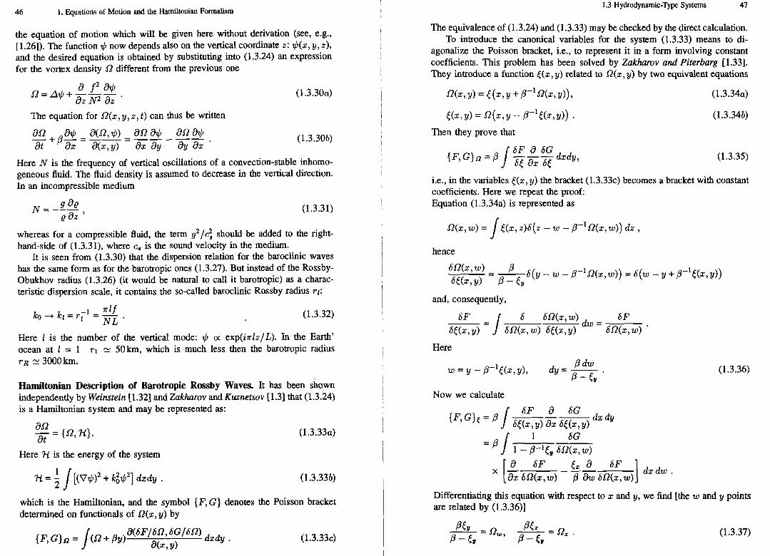
the equation of motion which will be given here without derivation (see, e.g., [1.26]). The function + now depends also on the vertical coordinate z: $(x, y, z), and the desired equation is obtained by substituting into (1.3.24) an expression for the vomx density L? different from the previous one
The equation for Q(x, y, z, t) can rhus be written
Here N is the frequency of vertical oscillations of a convection-stable inhomo- geneous fluid. The fluid density is assumed to decrease in the vertical direction. In an incompressible medium
whereas for a compressible fluid, the term 92/4 should be added to the right- hand-side of (1.3.31), where c, is the sound velocity in the medium.
It is seen from (1.3.30) that the dispersion relation for the baroclinic waves has the same form as for the barotropic ones (1.3.27). But instead of the Rossby- Obukhov radius (1.3.26) (it would be natural to call it barotropic) as a charac- teristic dispersion scale, it contains the so-called baroclinic Rossby radius rl:
Here 1 is the number of the vertical mode: 1C, IX exp(i~lz/L). In the Earth' ocean at I = 1 rl II 50km, which is much less then the barotropic radius rR II 3000 km.
Hamiltonian Description of Barotropic Rossby Waves. It has been shown independently by Weinstein (1.321 and Zakharov and Kuznetsov [1.3] that (1.3.24) is a Hamiltonian system and may be represented as:
Here 3C is the energy of the system
E = 5 [(v+)~ + k t$2] dxdy . / which is the Hamiltonian, and the symbol {F, G) denotes the Poisson bracket determined on functionals of R(x, y) by
a(SF/SQ, 6G/Sf2) dxdy .
a(x, Y)
The equivalence of (1.3.24) and (1.3.33) may be checked by the direct calculation. To introduce the canonical variables for the system (1.3.33) means to di-
agonalize the Poisson bracket, i.e., to represent it in a form involving constant coefficients. This problem has been solved by Zakharov and Piterbarg [1.33]. They introduce a function [(x, y) related to R(x, y) by two equivalent equations
&,Y) = Q(x,Y - P-*E(x,y)) . Then they prove that
i.e., in the variables ((x, y) the bracket (1.3.33~) becomes a bracket with constant coefficients. Here we repeat the proof: Equation (1.3.34a) is represented as
hence
Sfi(x,w) - P - -6(y - w - @-'52(x, w)) = 6(w - y + P-'((x, y)) S((X,Y) P - t#
and, consequently,
Here
Now we calculate
Differentiating this equation with respect to x and y, we find [the w and y points are related by (1.3.36)l
I- @( - nw, -= @(. nz P - l v P - Ev

2
tc
N
V
II $'I-
SM
-6
3 h
WW
%=-. 'm'
S h
a-
w
rn.. - a- - + 2
5 I ... - is.
w -
2
h
C :
00
V

1.4 Spin Waves 51 50 1. Equations of Motion and the Hamiltonian Formalism
In such terms the Hamiltonian (1.3.46) reduces to a form
Now we go over to normal canonical variables,
in which the Hamilton equation (1.3.40) takes the canonical form (1.3.42), and all that is left to do is to express the Hamiltonian (1.3.50) in terms of the normal variables. In view of the fact that for the Rossby waves, three-wave resonance interactions are possible, in calculating 'K we shall restrict ourselves to those terms that are quadratic and cubic in am(k). This allows us to use, instead of (1.3.47), an approximate relationship between 52 and ( which holds to an accuracy of the order of p-2.
Substitution of (1.3.51b) into (1.3.50) gives
+ Uk12 (a* a;a2+ - C.C) 6(k + k1 + kz)l dkdkidkz ,
If the vertical inhomogeneity is linear, then according to (1.3.31) N =const holds and
and for the coefficients (1.3.51~) we obtain
f B(m, ml, mz) = - NZ
It should be noted that in the case of the baroaopic waves, this expression is replaced by unity and k, by the constant ko.
1.4 Spin Waves
1.4.1 Magnetic Order, Energy and Equations of Motion
To date, a large variety of magnetically-ordered substances are known: dielectrics, semiconductors and metals, both crystalline and amorphous E1.351. Their struc- ture includes paramagnetic atoms (ions) with uncompensated spin S, thus having magnetic moment pS (p is the Bohr magneton here). Such atoms give rise to the exchange interaction which is of electrostatic nature and is to be associated with the Pauli principle prohibiting more than one electron to be in a given quantum- mechanical state E1.361. At low temperatures, this interaction leads to magnetic ordering orienting the magnetic moments of the atoms in a definite manner. The simplest type of magnetic ordering is the ferromagnetic state in which the mag- netic moments of all atoms are parallel. This results in a macroscopic magnetic moment with density M. In contrast to ferromagnets, the total magnetic moment of antiferromagnets is zero. In the simplest case, an elementary cell of crys- talline antiferromagnet has two magnetic atoms whose moments are antiparallel and equal in magnitude. In describing antiferromagnets one uses the notion of a magnetic sublattice, which contains the translational-invariant magnetic atoms, i.e., the positions of them differ by an integer number of elementary translations of the crystalline lattice. In the simplest antiferromagnet, there are two magnetic sublattices with the moments MI and M2, with M = M1 + M2 = 0.
At low temperatures the long-wave magnetic excitations may be described classically, using the functions M j ( ~ , t). These excitations are spin waves or precession waves of the magnetic moment. The equation of motion for M ( r , t) (the Bloch equation) describes the precession of a vector with a fixed length ( M ( T , t) 12= M ~ ( T ) =const in an effective magnetic field Heff(T,t) (see, e-g., [1.37]:

52 1. Equations of Motion and the Hamiltonian Formalism I 1.4 Spin Waves 53
Here g, = p/h is the ratio of magnetic to mechanical moment of the elec- trons, and W, the energy of the system. The g, value is approximately equal to 2 x 2 3 ~I-Iz/tj. The energy W is a functional of M ( T , t). In ferromagnets it includes Wo, the interaction energy of a spin subsystem with an external field H o , the exchange energy We, and a number of the terms of relativistic ori- gin. The main contributions stem from the energy of the magnetic dipole-dipole interaction Wdd and the energy of the crystalline anisotropy W,,:
W,, = K M Z ~ T , J (1.4.2d) I
Here t c tk and K are material constants; Hm is the static magnetic field created by the magnetic moment distribution. The phenomenological expression (1.4.2) for the energy of a ferromagnet is discussed in detail in [1.37-381. Here we shall
I only comment on it in brief. The physical meaning of Wo is obvious, it is the magnetic dipole energy in the external field H ; the integral in the expression ~
I for Wdd defines the dipole energy in the self-magnetic field H,, with the in- teraction energy of each pair taken into account twice. The factor ; in (1.4.2e) compensates for this double counting. The expression (1 .42 ) for We, is general enough. Indeed, if we suggest that (i) We, is independent of the magnetization relative to the crystal axes; (ii) the crystal has an inverted symmetry element; (iii) the energy dependence on the magnetization is quadratic. For the derivation of (1.4.2~) see, e.g., [1.37]. Item (i) follows from the nature of the exchange interaction which is invariant relative to the total rotation of all spins. (ii) is
I I I
satisfied since most magnets are just of this kind. (iii) holds strictly speaking I
only for magnetic atoms with the spin S = 112. At S > 112 this suggestion I is invalid, but experiment shows that corrections to (1.4.2~) are small and this 1 has been theoretically substantiated [1.39]. The term (1.4.2d) for the crystalline
I
anisotropy energy appears in second order perturbation theory with regard to the spin-orbit interaction as a weak one. The constant K is nonzero for uniaxial crystals. At K < 0, the energetically favorable orientation of magnetization is that along the crystal's symmetry axis ( z axis). At K > 0 the orientation in the
~ I 1
plane perpendicular to the z axis is favored. In the former case, the anisotropy is referred to as being of the easy axis type, and in the latter case, it is said to be of the easy plane type. Finally, in crystals with a cubic symmetry, the expression for t c ;k is simplified compared with that for the isoeopic continuous medium K t k = ~ 6 , ~ .
1.4.2 Canonical Variables
In (1.4.1) we go over to circular variables
We choose the z axis along the equilibrium direction of magnetization. Then at small oscillation amplitudes of the magnetic moment the M* values will be small, and M, will be close to the length of M , i.e., Mo. Comparing (1.4.3) and (1.1.6), we see that these equations have in the M*-linear approximation the form of Hamilton equations if we take as the canonical variables
M+ M- a ( ~ , t) = &G'J%'
a*(r , t )= - . d 2 g d f o
Therefore it is reasonable to write these canonical variables as
Substituting (1.4.4) into (1.4.3), we obtain an equation for &(T, t)/&:
Here
Demanding these equations to coincide with the canonical equations (1.1.6), we obtain the differential equation for the function f (x)
of which the only solution satisfying the condition f (0) = 1 is
Thus we have expressed the natural variables of the ferromagnet's spin subsystem M,, M* through the canonical ones:
This equation is nonlinear and valid if g,a*a < 2Mo. The ferromagnet's energy W expressed via the canonical variables becomes the Hamiltonian %(a*, a). In quantum mechanics, the Holstein-Primakoff representation has long been known [1.37-381. It gives the spin operators in terms of Bose operators. The formulas (1.4.7) are the classical analogue of this representation. They were first used by
P Pi s
n
k
g "w
2
II h
)l I-.
a &
& !s q " g
Q
n
$4
9s.
". 5
$ 5'
5
n
!--
3-
8 >
- a
X
'd, fj.
w
?i' r \ 3- - n
C
:A r: s

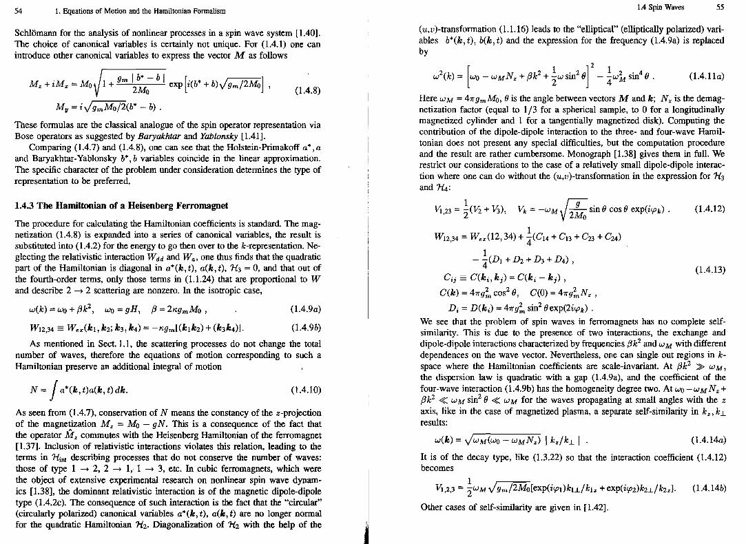
56 1. Equations of Motion and the Hamiltonian Formalism
1.4.4 The Hamiltonian of Antiferrornagnets
The simplest antiferromagnets have two magnetic sublattices and, accordingly, two spin wave branches. The quadratic part of the Hamiltonian has the standard form (1.1.17)
We give this expression here to introduce the notations for the spin wave fre- quencies in the two branches w(k), Q(k) and the normal canonical variables a k = a(k, t), a; = a*(k, t). In the uniaxial ferromagnets with an "easy axis"-type anisotropy, the (crystalline) anisotropy field Ha tends to keep the magnetization parallel to that axis (usually called the z axis).
By analogy with ferromagnets, spin wave frequencies with k + 0 would be expected to correspond to sublattice magnetization precession in the field H a , i.e.
where
However this is not so. In fact, the magnetization of the sublattice MI oriented upwards is affected by the anisotropy field Hal which is also oriented upwards: Hal = Ha. The second sublattice M2 = -MI is affected by another field Ha2 = -Hal. AS a result, the sublattices tend to precess in opposite directions. In this case, the antiparallel arrangement of M1 and M2 will inevitably be broken up, which is prevented by the strong exchange interaction between sublattices. As a result we have [1.37]
Here we, = g, B M characterizes the antiferromagnetic exchange between sublat- tices. The order of magnitude of the dimensionless exchange constant is B 11 lo3.
In uniaxial antiferromagnets with "easy planew-type anisotropy, the ani- sotropic field rotates the sublattice moments into the plane perpendicular to the z axis. The possibility of almost free oscillations of moments in this plane leads to the fact that one of the spin wave frequencies at k = 0 turns out to be small, i.e., wo 11 w ~ . The upper branch gap lies much higher:
This situation is of special interest for experiments on the nonlinear properties of spin waves: the investigated frequency range below SOGHz includes the lower branch wk. Thus for "easy-plane" antiferromagnets we write down the results for the Hamiltonian coefficients in question [1.38]:
1.4 Spin Waves 57
We used the shorthand notation
I
I 0i = Q(ki), W, = ~ ( k i ) , wi-j = w(ki - kj), etc .
It should be borne in mind that a scattering process of type 2 + 2 does not just require to take into account the Hamiltonian 'H4 but also N3 in second order perturbation theory. It may be shown that the dominant contribution to the wk/we, parameter will be due to processes involving the upper-branch virtual wave, as explicitly given in (1.4.19). Using (1.1.29), we can derive an expression for the effective coefficient of the lower branch four-wave processes T [1.38]. The general expression for T is rather cumbersome. For k1 = k3, k2 = k4, wl = w2 = wg = w4 it reads
It is evident from these formulas that the problem of spin waves in an- tiferromagnets does not possess complete self-similarity, like in ferromagnets.
I However, a second-order self-similarity does exist. Thus in the dispersion law (1.4.18), three regions may be singled out. At k -+ 0, the wk and 0 k branches have a gap with a quadratic addition. In the region of large k, the functions wk and flk follow a linear law. Since usually waw,, >> w&, there is an intermediate range of the k values where the frequency wk has already become asymptotically linear and Qk = 520 + ,f3k2. We shall not go through the simple but cumbersome analysis of the asymptotics of the interaction coefficient (1.4.16, 17). We shall only note that at k + 0, the coefficient of the four-wave interaction becomes constant. In this case the Hamiltonian of the problem for low-frequency waves has an especially simple form:

58 1. Equations of Motion and the Hamiltonian Formalism
Why have we taken into account the term cc k2 in the expression for wk but neglected it in the expression for T = To + O(k2) although it has in fact the same relative order of magnitude? The answer is: the constant wo is not involved in the problem and is eliminated by the time-dependent canonical transformation
In the variables c(k,t), the Hamiltonian (1.4.21) has the form:
The respective dynamic equation idc(k, t)/dt = 63-1/6c(k, t) has after the in- verse Fourier transform c(k, t) -+ $(T, t) the form of the nonlinear Schrodinger equation
Indeed, that is the quantum mechanical Schrodinger equation with 1 + 1 2 as a potential.
1.5 Universal Models
The nonlinear Schrodinger equation which we encountered at the end of the previous section is a member of a small family of famous universal equations that arise in the nonlinear wave theory. Every such equation describes a large variety of physical systems belonging to different topics of physics. As we shall show just now, the nonlinear Schrijdinger equation describes the behavior of a narrow wave packet envelope for most nonlinear wave systems, see Sect. 1.5.1. If we consider another physical situation, namely long-wave perturbations of the acoustic type (which can exist in most media), then we obtain the well-known Korteweg - de Vries (KdV) equation in the one-dimensinal case and the rather fa- mous Kadomtsev-Petviashvili equation for weakly two-dimensional distributions, see Sect. 1.5.2. In Sect. 1.5.3 we shall consider a third rather universal physical situation: the interaction of three-wave packets in media with a decay dispersion law. All three of these models have extremely wide applications, ranging from solid state physics to hydrodynamics, plasma physics, etc.
1.5 Universal Models 59
1.5.1 Nonlinear Schrodinger Equation for Envelopes
This equation, like the Hamiltonian (1.4.23), has a wide range of applications. Basically, these applications are associated with the fact that (1.4.24) describes the behavior of an envelope of quasi-monochromatic waves in isotropic nonlinear media. Equation (1.4.24) should be regarded as written in a reference system moving with the group velocity of a wave packet.
Now let us show how the dynamical equation (1.4.24) can be obtained for a narrow wave packet. If the carrier wave vector is denoted by ko and )k - kol =
I K / << ko, we assume
to hold. Here v = ( d ~ / d k ) ~ = ~ ~ is the group velocity. In isotropic media, with the frequency depending only on the modulus of the wave vector, the third term in (1.5.1) can be simplified
In the propagation of a single narrow envelope the three-wave interaction is not important (but it must be taken into account in higher-order perturbation theory). Waves with approximately equal wave vectors are involved in the four-wave interaction. The dynamic equation has the form
For a narrow packet it can be assumed that
Introducing the envelope of the quasi-monochromatic wave
$(T, t) = ( 2 ~ ) - ~ ' ~ exp[i(koT) - iw(ko)t] / c(ko + rc, t)exp[i(rc~)]dn
and making the inverse Fourier transform in (1.5.2), we amve at
The z-axis is chosen in the direction of the wave propagation. The second term in (1.5.3) can be eliminated by the transition to a reference system moving with the group velocity: z -+ z - vt. Expanding the z-coordinate according to z -+ z(~oEow"/v)~I~ and using A = A L + $/az2, one can reduce (1.5.3) to

60 1. Equations of Motion and the Harniltonian Formalism 15 Universal Models 6 1
(1.4.24). It should be noted that (1.5.3) can be considered both for three- and two-dimensional media. The latter applies mainly to water wave envelopes.
In deriving (1.5.3) we assume that the coefficient T(k, kl, k2, k3) is a con- tinuous function when all the arguments tend to ko. This is not always true; in some cases, this limit depends on the direction of the vector k with respect to the direction of ko. In such cases (1.5.3) should be replaced by a more complicated equation.
However in most of the isotropic media the behavior of envelopes is governed by (1.5.3). In particular, this equation describes self-focussing of light in nonlinear dielectrics [1.43] and the quasi-classical limit of a weakly nonhomogeneous Bose gas [1.44-45]. It should also be noted that the coefficient To may be either positive (corresponding to the effective attraction of quasi-particles) or negative (corresponding to their repulsion). Scale transformations of the coordinates and the field $ may be used to obtain unity for the values of the parameters P and TO. The turbulence of envelopes is sometimes called optical turbulence because nonlinear optics is a field with a multitude of applications for nonlinear wave theory.
1.5.2 Kadomtsev-Petviashvili Equation for Weakly Dispersive Waves
Let us consider a hydrodynamic type system with the usual Hamiltonian
where the internal energy E, is connected with the densih variation p = po + be and has the form (1.2.18,21)
Such a Hamiltonian expansion using the smallness of nonlinearity and dispersion is quite universal [for example, we obtain the equations of the ion sound in plasmas (1.3.10) with such an approximation]. Respective dynamical equations have the standard form (1.2.8-9):
The right-hand-sides of these equations contain the small effects of nonlinear- ity and dispersion while the left-hand-side describes the main phenomenon: the motion of a perturbation with the sound velocity (vtt - ~ A V = 0). We can eliminate the latter by going over to a moving reference frame. Let the x- axis coincide with the direction of motion of the sound velocity. We suppose
v x v, = v, av/dx >> dv/ay, &/dz and the same inequality for SQ. Sub- stituting into the terns on the right the zero-order relations 6et = -@ div v = pov,, vt = - 4 ~ b p / @ , we obtain
Here the terns on the left-hand-side are much greater than those on the right- hand-side. We introduce instead of x, t the slow variables ( = x - vt and slow
a a a a a a time r, so we can substitute vtt - v,, = ( z - c,=)(% + cSE)v = 2%=v to obtain finally the Kadomtsev-Petviashvili equation [1.46]
As it is clear from its derivation, this equation is valid in the case of weak nonlinearity (v << c,), weak dispersion (pv,, << v) and small deviations from one-dimensionality (v, >> Vlv). In the truncated equation all terms are generally of the same order, since linear effects are excluded. Following (1.2.17), one can introduce for (1.5.4) normal canonical variables with v = V@. So we obtain
Peo cs w(k, , kI) = - ki + -kt , 2c, 2k,
For purely one-dimensional motions the Kadomtsev-Petviashvili equation re- turns to the famous KdV equation:
1.5.3 Interaction of Three Wave Packets
Let us discuss the interaction of three narrow wave packets with characteristic wave vectors kl , k2 and kg. For this interaction to be essential, it is necessary that these vectors should lie in the vicinity of the resonant surface w(k1 + k2) = w(kl) + w(k2). Let us represent the wave amplitude c(k, t) as
and, making use of the narrowness of the packets ( K << kj), expand the function w(k) :
The value c(8,t) obeys the usual dynamic equation for the three-wave case
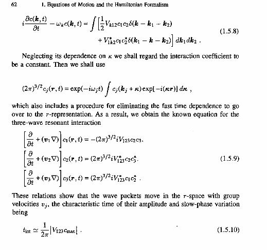
62 1. Equations of Motion and the Hamiltonian Formalism
Neglecting its dependence on rc we shall regard the interaction coefficient to be a constant. Then we shall use
( ~ T ) ~ / ~ c ~ ( T , t) = exp(-iwjt) ci(kj + rc)exp[-i(rcr)] drc , J which also includes a procedure for eliminating the fast time dependence to go over to the r-representation. As a result, we obtain the known equation for the three-wave resonant interaction
These relations show that the wave packets move in the r-space with group velocities vj, the characteristic time of their amplitude and slow-phase variation being
1 tint -JVj~cmaxl .
27T
2. Statistical Description of Weak Wave Thrbulence
It is a thing which you can easily explain twice before anybody knows what you are talking about
A. Milne "The House at Pooh Corner"
In this chapter we shall go over from the dynamic description of wave systems to the statistical one. This will be done in terms of pair correlators of a wave field. They represent the occupation numbers (density) of waves in k-space. In Sect. 2.1 we shall obtain the kinetic equation for the occupation numbers of waves as the main mathematical objects dealt with in the first volume of this book. In Sect. 2.2 we shall study the general properties of these equations and derive the stationary equilibrium solutions. Section 2.2.3 deals with the general necessary conditions for the existence of Kolmogorov spectra.
2.1 Kinetic Wave Equation
2.1.1 Equations of Motion
In the preceding chapter we have applied the Harniltonian method to the motion in continuous media like fluids, plasmas, solids and the planetary atmosphere, have considered the structure of the Hamiltonian for weak nonlinearities and given its coefficients for some physical examples. The canonical equation of motion in terms of complex wave amplitudes c(k, t), i.e.,
is the main result. After application of the procedure outlined in Sect. 1.1.3, the interaction Harniltonian 'Hint includes only the terms describing real processes for which the energy and momentum conservation laws are valid. If a medium supports propagating waves for which three-wave decay processes are allowed, we have:
In this case