Kolmogorov, Fomin, Elements of the Theory of Functions and Functional Analysis. Volume 1 Metric and...
141
-
Upload
luis-perdomo-hurtado -
Category
Documents
-
view
1.653 -
download
10
description
Mathematical analysis Kolmogoroc
Transcript of Kolmogorov, Fomin, Elements of the Theory of Functions and Functional Analysis. Volume 1 Metric and...


ELEMENTS OF THE THEORY OF FUNCTIONS
AND FUNCTIONAL ANALYSIS
VOLUME 1
METRIC AND NORMED SPACES

OTHER GRAYLOCK PUBLICATIONS
ALEKSANDROV: Combinatorial Topology Vol. 1: Introduction. Complexes. Coverings. Dimension Vol. 2: The Betti Groups Vol. 3: Homological Manifolds. The Duality Theorems. Cohomology Groups of Compacta. Continuous MapPings of Polyhedra
KHlNCHIN: Three Pearls of Number Theory Mathematical Foundations of Quantum Statistics
KOLMOGOROV and FOMIN: Elements of the Theory of Functions and Functional Analysis Vol. 1: Metric and Normed SPaces Vol. 2: Measure. The Lebesgue Integral. Hilbert Space
NOVOZHILOV: Foundations of the Nonlinear Theory of Elasticity
PETROVSKII: Lectures on the Theory of Integral Equations
PONTRYAGIN: Foundations of Combinatorial Topology

Elements of the Theory of Functions
and Functional Analysis
VOLUME 1
METRIC AND NORM ED SPACES
BY A. N. KOLMOGOROV AND S. V. FOMIN
rRANSLATED FROM THE FIRST (1954) RUSSIAN EDITION
by
LEO F. BORON Department of Mathematics
University of Wisconsin
GRAYLOCK PRESS
ROCHESTER, N. Y.
1957

Copyright, 1957, by GRAYLOCK PRESS
Rochester, N. Y.
All rights reserved. This book, or parts thereof, may not be reproduced in any form, or translated, without permission in writing from the publishers.
Library of Congress Catalog Card Number 57-14021
Third Printing, July 1963
Ma .... factured i.. lAo U .. iled Stale. 0/ America
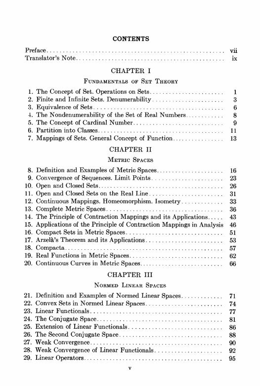
CONTENTS
Preface ...................................................... . vii Translator's Note. . . . . . . . . . . . . . . . . . . . . . . . . . . . . . . . . . . . . . . . . . . . .. IX
CHAPTER I
FUNDAMENTALS OF SET THEORY
1. The Concept of Set. Operations on Sets. . . . . . . . . . . . . . . . . . . . . . . 1 2. Finite and Infinite Sets. Denumerability. . . . . . . . . . . . . . . . . . . . . . 3 3. Equivalence of Sets. . . . . . . . . . . . . . . . . . . . . . . . . . . . . . . . . . . . . . . . 6 -I" The Nondenumerability of the Set of Real Numbers. . . . . . . . . . . . 8 .5. The Concept of Cardinal Number.. . . . . . . . . . . . . . . . . . . . . . . . . . . 9 6. Partition into Classes. . . . . . . . . . . . . . . . . . . . . . . . . . . . . . . . . . . . . .. 11 7. Mappings of Sets. General Concept of Function. . . . . . . . . . . . . . .. 13
CHAPTER II
METRIC SPACES
8. Definition and Examples of Metrio Spaces. . . . . . . . . . . . . . . . . . . .. 16 9. Convergence of Sequences. Limit Points. . . . . . . . . . . 23
10. Open and Closed Sets. . . . . . . . . . . . . . . . . . . . . . . . . . . . . . . . . . . . . .. 26 11. Open and Closed Sets on the Real Line. . . . . . . . . . . . . . . . . . . . . .. 31 12. Continuous Mappings. Homeomorphism. Isometry. . . . . . . . . . . .. 33 13. Complete Metric Spaces. . . . . . . . . . . . . . . . . . . . . . . . . . . . . . . . . . .. 36 14. The Principle of Contraction Mappings and its Applications. . . .. 43 15. Applications of the Principle of Contraction Mappings in Analysis 46 16. Compact Sets in Metric Spaces. . . . . . . . . . . . . . . . . . . . . . . . . . . . .. 51 17. ArzeUt's Theorem and its Applications. . . . . . . . . . . . . . . . . . . . . . .. 53 18. Compacta... . . . . . . . . . . . . . . . . . . . . . . . . . . . . . . . . . . . . . . . . . . . . .. 57 19. Real Functions in Metric Spaces. . . . . . . . . . . . . . . . . . . . . . . . . . . .. 62 20. Continuous Curves in Metric Spaces.... . . . . . . . . . . . . . . . . . . . . .. 66
CHAPTER III
NORMED LINEAR SPACES
21. Definition and Examples of Normed Linear Spaces. . . . . . . . . . . .. 71 22. Convex Sets in N ormed Linear Spaces. . . . . . . . . . . . . . . . . . . . . . .. 74 23. Linear Functionals. . . . . . . . . . . . . . . . . . . . . . . . . . . . . . . . . . . . . . . .. 77 24. The Conjugate Space. . . . . . . . . . . . . . . . . . . . . . . . . . . . . . . . . . . . . .. 81 25. Extension of Linear Functionals. . . . . . . . . . . . . . . . . . . . . . . . . . . .. 86 26. The Second Conjugate Space. . . . . . . . . . . . . . . . . . . . . . . . . . . . . . .. 88 27 . Weak Convergence. . . . . . . . . . . . . . . . . . . . . . . . . . . . . . . . . . . . . . . .. 90 28. Weak Convergence of Linear Functionals. . . . . . . . . . . . . . . . . . . .. 92 29. Linear Operators.. . . . . . . . . . . . . . . . . . . . . . . . . . . . . . . . . . . . . . . . .. 95
v

VI CONTENTS
ADDENDUM TO CHAPTER III
GEXERALIZED FUNCTIONS
CHAPTER IV
LINEAH OPERATOR EQUATIONS
:30. Spectrum of an Operator. Resolvents. . . . . . . . . . . . . . . . . . . . . 110 31. Completely Continuous Operators ............................ 112 32. Linear Operator Equations. Fredholm's Theorems.. . . . . . . . 116 LIST OF SyMBOLS.... . . . . . . . . . . . . . . . . . . . . . . . . . . . . . . . . . . . . . . . . .. 122 LIST OF DEFINITIONS. . . . . . . . . . . . . . . . . . . . . . . . . . . . . . . . . . . . . . . . .. 123 LIST OF THEOREMS.. . . . . . . . . . . . . . . . . . . . . . . . . . . . . . . . . . . . . . . . . .. 123 BASIC LIn;RATuRE ............................................ 125 INDl';X ........................................................ 127

PREFACE
The present book is a revised version of material given by the authors in two courses at the Moscow State University. A course in functional analysis which included, on the one hand, basic information about the theory of sets, measure and the Lebesgue integral and, on the other hand, examples of the applications of the general methods of set theory, theory of functions of a real variable, and functional analysis to concrete problems in classical analysis (e.g. the proof of existence theorems, the discussion of integral equations as an example of a special case of the theory of operator equations in linear spaces, etc.) was given by the first author, A. N. Kolmogorov, in the Department of Mathematics and Mechanics. A somewhat less comprehensive course was given by the second author, S. V. Fomin, for students specializing in mathematics and theoretical physics in the Department of Physics. A. A. Petrov's notes of A. X. Kolmogorov's leetures were used in a number of sections.
The material included in the first volume is clear from the table of contents. The theory of measure and the Lebesgue integral, Hilbert space, theory of integral equations with symmetric kernel and orthogonal systems of functions, the elements of nonlinear functional analysis, and some applications of the methods of functional analysis to problems arising in the mathematics of numerical methods will he considered in later volumes.
February 1954
vii
A. KOLMOGOROV
R. FOMIN


TRANSLATOR'S NOTE This volume is a translation of A. N. Kolmogorov and S. V. Fomin's
Elementy Teorii Funkci'i i Funkcional'nogo Analiza., I. Metriceskie i Normirovannye Prostranstva. Chapter I is a brief introduction to set theory and mappings. There is a clear presentation of the elements of the theory of metric and complete metric spaces in Chapter II. The latter chapter also has a discussion of the principle of contraction mappings and its applications to the proof of existence theorems in the theory of differential and integral equations. The material on continuous curves in metric spaces is not usually found in textbook form. The elements of the theory of normed linear spaces are taken up in Chapter III where the Hahn-Banach theorem is proved for real separable normed linear spaces. The reader interested in the extension of this theorem to complex linear spaces is referred to the paper Extension oj Functionals on Complex Linear Spaces, Bulletin AMS, 44 (1938), 91-93, by H. F. Bohnenblust and A. Sobczyk. Chapter III also deals with weak sequential convergence of elements and linear functionals and gives a discussion of adjoint operators. The addendum to Chapter III discusses Sobolev's work on generalized functions which was later generalized further by L. Schwartz. The main results here are that every generalized function has derivatives of all orders and that every convergent series of generalized functions can be differentiated term by term any number of times. Chapter IV, on linear operator equations, discusses spectra and resolvents for continuous linear operators in a complex Banach space. Minor changes have been made, notably in the arrangement of the proof of the Hahn-Banach theorem. A bibliography, listing basic books covering the material in this volume, was added by the translator. Lists of symbols, definitions and theorems have also been added at the end of the volume for the convenience of the reader.
Milwaukee 1957 Leo F. Boron
ix


Chapter I
FUNDAMENTAL CONCEPTS OF SET THEORY
§1. The concept of set. Operations on sets
In mathematics as in everyday life we encounter the concept of set. We can speak of the set of faces of a polyhedron, students in an auditorium, points on a straight line, the set of natural numbers, and so on. The concept of a set is so general that it would be difficult to give it a definition which would not reduce to simply replacing the word "set" by one of the equivalent expressions: aggregate, collection, etc.
The concept of set plays an extraordinarily important role in modern mathematics not only because the theory of sets itself has become at the present time a very extensive and comprehensive discipline but mainly because of the influence which the theory of sets, arising at the end of the last century, exerted and still exerts on mathematics as a whole. Here we shall briefly discuss only those very basic set-theoretic concepts which will be used in the following chapters. The reader will find a significantly more detailed exposition of the theory of sets in, for example, the books by P. S. Aleksandrov: Introduction to the General Theory of Sets and Functions, where he will also find a bibliography for further reading, E. Kamke: Theory of Sets, F. Hausdorff': Mengenlehre, and A. Fraenkel: Abstract Set Theory.
We shall denote sets by upper case letters A, B, ... and their elements hy lower case letters a, b, .... The statement "the element a belongs to the set A" will be written symbolically as a E A.; the expression a (£ A means that the element a does not belong to the set A. If all the elements of which the set A consists are also contained in the set B (where the case A = B is not excluded), then A will be called a subset of B and we shall write A ~ B. (The notation A c B denotes that A is a subset of the set B and A ~ B, i. e. there exists at least one element in B which does not belong to A. A is then said to be a proper subset of the set B.) For example, the integers form a subset of the set of real numbers.
Sometimes, in speaking about an arbitrary set (for example, about the set of roots of a given equation) we do not know in advance whether or not this set contains even one element. For this reason it is convenient to introduce the concept of the so-called void set, that is, the set which does not contain any elements. We shall denote this set by the symbol O. Every set contains 0 as a subset.
If A and B are arbitrary sets, then their sum or union is the set C =
A U B consisting of all elements which belong to at least one of the sets A. and B (Fig. 1).
1

2
A
FUNDAMENTALS OF SET THEORY
B A B
C·A"B FIG. 2
[CH. I
We define the sum of an arbitrary (finite or infinite) number of sets analogously: if Aa are arbitrary sets, then their sum A = Ua Aa is the totality of elements each of which belongs to at least one of the sets Aa.
The inter8ection of two sets A and B is the set C = A n B which consists of all the elements belonging to' both A and B (Fig. 2). For example, the intersection of the set of all even integers and the set of all integers which are divisible by three is the same as the set of all integers which are divisible by six. The intersection of an arbitrary (finite or infinite) number of sets Aa is the set A = na Aa of all elements which belong to all of the sets Aa . If A n B = 8, we shall say that A and B are disjoint. The same term will apply to any collection of sets {A a} for which All n A'Y = 8, f3 ¢ 'Y.
The operations of union and intersection are connected by the following relations:
(1)
(2)
(A U B) n C = (A n C) U (B n C),
(A n B) U C = (A U C) n (B U C).
We shall verify the first of these two relations. Let the element x belong to the set on the left side of equation (1). This means that x belongs to C and moreover that it belongs to at least one of the sets A and B. But then x belongs to at least one of the sets A n C and B n C, i.e. it belongs to the right member of equation (1). To prove the converse, let x E (A n C) U (B n C). Then x E A n C and/or x E B n C. Consequently, x E C and, moreover, x belongs to at least one of the sets A and B, i. e. x E (A U B). Thus we have shown that x E (A U B) n C. Hence, equation (1) has been verified. Equation (2) is verified analogously.
We define further the operation of subtraction for sets. The difference of the sets A and B is the set C = A"'" B of those elements in A which are not contained in B (Fig. 3). In general it is not assumed here that A :::> B.
In some instances, for example in the theory of measure, it is convenient to consider the so-called symmetric difference of two sets A and B; the symmetric difference is defined as the sum of the differences A "'" Band B "'" A (Fig. 4). We shall denote the symmetric difference of the sets A and B by

§2) FINITE AND INFINITE SETS. DENUMERABILITY 3
A A B
the symbol A~B. Its definition is written symbolically as follows:
A~B = (A '" B) U (B '" A). EXERCISE. Show that A~B = (A U B) '" (A n B). In the sequel we shall frequently have occasion to consider various sets
all of which are subsets of some fundamental set S, such as for example various point sets on the real line. In this case the difference S'" A is called the complement of the set A with respect to S.
In the theory of sets and in its applications a very important role is played by the so-called principle of duality which is based on the following two relations.
1. The complement of a sum is equal to the intersection of the complements,
(3) s'" U .. A .. = n .. (S", A .. ). 2. The complement of an intersection is equal to the sum of the complements,
(4) S '" n .. A .. = U .. (S '" A .. ).
By virtue of these relations, we can start with an arbitrary theorem concerning a system of subsets of a fixed set S and automatically obtain the dual theorem by replacing the sets under consideration by their complements, sums by intersections, and intersections by sums. Theorem 1', Chapter II, §1O, is an example of the application of this principle.
We shall now prove relation (3). Let xES'" U .. A ... This means that x does not belong to the sum U .. A .. , i.e. x does not belong to any of the sets A .. . Consequently, x belongs to each of the complements S'" A .. and therefore x E n .. (S '" A .. ). Conversely, let x E n .. (S '" A .. ), i.e. x belongs to every S '" A .. . Consequently, x does not belong to any of the sets A .. , i.e. it does not belong to their sum U .. A .. . But then xES", U .. A .. ; this concludes the proof of (3). We prove relation (4) analogously.
§2. Finite and infinite sets. Denumerability
In considering various sets we note that for some of them we can indicate the number of elements in the set, if not actually then at least in theory. Such, for example, is the set of chairs in a given room, the set of pencils in a box, the set of all automobiles in a given city, the set of all

FUNDAME;)JTALS OF SET THEORY [CH. I
molecules of water on the earth, and so on. Each of these sets contains a finite number of elements, although the number may not be known to us. On the other hand, there exist sets consisting of an infinite number of elements. Such, for example, are the sets of all natural numbers, all pointR on the real line, all circles in the plane, all polynomials with rational coefficients, and so forth. In this connection, when we say that a set is infinite, we have in mind that we can remove one element, two elements, and so on, where after each step elements still remain in the set.
When we consider two finite sets it may occur that the number of elements in both of them is the same or it may occur that in one of these sets the number of elements is greater than in the other, i.e. we can compare finite sets by means of the number of elements they contain. The question can be asked whether or not it is possible in a similar way to compare infinite sets. In other words, does it make sense, for example, to ask which of the following sets is the larger: the set of circles in the plane or the set of rational points on the real line, the set of functions defined on the segment [0, 1] or the set of straight lines in space, and so on?
Consider more carefully how we compare two finite sets. We can tackle the problem in two ways. We can either count the number of elements in each of the two sets and thus compare the hvo sets or we can try to establish a correspondence between the elements of these sets by assigning to each element of one of the sets one and only one element of the other set, and conversely; such a correspondence is said to be one-to-one. Clearly, a one-to-one correspondence between two finite sets can be established if and only if the number of elements in both sets is the same. For instance, in order to verify that the number of students in a group and the number of seats in an auditorium are the same, rather than counting each of the sets, one can seat each of the students in a definite seat. If there is a sufficient number of seats and no seat remains vacant, i.e. if a one-to-one correspondence is set up between these two sets, then this will mean that the number of elements is the same in both.
But it is obvious that the first method (counting the number of elements) is suitable only for comparing finite sets, whereas the second method (setting up a one-to-one correspondence) is suitable to the same degree for infinite as well as for finite sets.
Among all possible infinite sets the simplest is the set of natural numbers. We shall call every set whose elements can be put into one-to-one correspondence with all the natural numbers a denumerable set. In other words, a denumerable set is a set whose elements can be indexed in the form of an infinite sequence: al, ll2, ... , a", .... The following are examples of denumerable sets.
1. The set of all integers. We can establish a one-to-one correspondence

§2) FINITE AND INFINITE SETS. DENUMERABILITY 5
between the set of all integers and the set of all natural numbers in the following way:
o -1 1 1 2 3
-2 2 4 5
where in general we set n - 2n + 1 if n ~ 0 and n - - 2n if n < O. 2. The set of all positive even integers. The correspondence is obviously
n-2n. 3. The set of numbers 2, 4, 8, ... , 2n , •••• Assign to each number
2n the corresponding n; this correspondence is obviously one-to-one. 4. We now consider a slightly more complicated example: we shall
show that the set of all rational ,numbers is denumerable. Every rational number can be written in the form of an irreducible f~action a = p/q, q > O. Call the sum n = I p I + q the height of the rational number a. It is clear that the number of fractions having height n is finite. For instance, the number 0/1 = 0 is the only number having height 1; the numbers 1/1 and -1/1 are the only numbers having height 2; the numbers 2/1, 1/2, -2/1 and -1/2 have height 3; and so forth. We enumerate all the rational numbers in the order of increasing heights, i.e. first the numbers with height 1, then the numbers with height 2, etc. This process assigns some index to each rational number, i.e. we shall have set up a one-to-one correspondence between the set of all natural numbers and the set of all rational numbers.
An infinite set which is not denumerable is said to be a nondenumerable set.
We establish some general properties of denumerable sets. 1°. Every subset of a denumerable set is either finite or denumerable. Proof. Let A be a denumerable set and let B be a subset of A. If we
enumerate the elements of the set A: al , a2, ... , an, ... and let nl, n2 , ... be the natural numbers which correspond to the elements in B in this enumeration, then if there is a largest one among these natural numbers, B is finite; in the other case B is denumerable.
2°. The sum of an arbitrary finite or denumerable set of denumerable sets is again a finite or denumerable set.
Proof. Let AI, A 2, .,. be denumerable sets. All their elements can be written in the form of the following infinite table:
an al2 al3 al4 a2l a22 ~ aM a31 a32 aaa aM au a42 a43 a« ...................
where the elements of the set Al are listed in the first row, the elements

6 FUNDAMENTALS OF SET THEORY [CH. I
of A2 are listed in the second row, and so on. We now enumerate all these elements by the "diagonal method", i.e. we take an for the first element, a12 for the second, ~l for the third, and so forth, taking the elements in the order indicated by the arrows in the following table:
an -+ a12 al3 -+ au·· . ./ )" ./
a21 a22 a23 a24·· . ! )" ./
a31 a32 a33 a34·· . ./
a41 a42 a43 a44· .. .................. . ..
It is clear that in this enumeration every element of each of the sets Ai receives a definite index, i.e. we shall have established a one-to-one correspondence between all the elements of all the AI, A 2 , ••• and the set of natural numbers. This completes the proof of our assertion.
EXERCISES. 1. Prove that the set of all polynomials with rational coefficients is denumerable.
2. The number ~ is said to be algebraic if it is a zero of some polynomial with rational coefficients. Prove that the set of all algebraic numbers is denumerable.
3. Prove that the set of all rational intervals (i.e. intervals with rational endpoints) on the real line is denumerable.
4. Prove that the set of all points in the plane having rational coordinates is denumerable. Hint: Use Theorem 2°.
3°. Every infinite 8et contain8 a denumerable sub8et. Proof. Let M be an infinite set and consider an arbitrary element al in M.
Since M is infinite, we can find an element a2 in M which is distinct from al , then an element a3 distinct from both al and ~ , and so forth. Continuing this process (which cannot terminate in a finite number of steps since M is infinite), we obtain a denumerable subset A = {aI, a2, a3, ... j of the set M. This completes the proof of the theorem.
This theorem shows that denumerable sets are, so to speak, the "smallest" of the infinite sets. The question whether or not there exist nondenumerable infinite sets will be considered in §4.
§3. Equivalence of sets
We arrived at the concept of denumerable set by establishing a oneto-one correspondence between certain of infinite sets and the set of natural numbers; at the same time we gave a number of examples of denumerable sets and some of their general properties.
§3] EQUIVALENCE OF SETS 7
It is clear that by setting up a one-to-one correspondence it is possible not only to compare infinite sets with the set of natural numbers; it is possible to compare any two sets by this method. We introduce the following definition.
DEFINITION. Two sets M and N are said to be equivalent (notation: M ("-.J N) if a one-to-one correspondence can be set up between their elements.
The concept of equivalence is applicable to arbitrary sets, infinite as well as finite. It is clear that two finite sets are equivalent if, and only if, they consist of the same number of elements. The definition we introduced above of a denumerable set can now be formulated in the following way: a set is said to be denumerable if it is equivalent to the set of natural numbers.
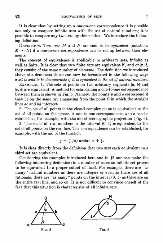
ExAMPLES. 1. The sets of points on two arbitrary segments [a, b] and [e, d] are equivalent. A method for establishing a one-to-one correspondence between them is shown in Fig. 5. Namely, the points p and q correspond if they lie on the same ray emanating from the point 0 in which the straight lines ac and bd intersect.
2. The set of all points in the closed complex plane is equivalent to the set of all points on the sphere. A one-to-one correspondence a ~ z can be established, for example, with the aid of stereographic projection (Fig. 6).
3. The set of all real numbers in the interval (0, 1) is equivalent to the set of all points on the real line. The correspondence can be established, for example, with the aid of the function
y = (l/7r) arctan x + i. It is clear directly from the definition that two sets each equivalent to a
third set are equivalent. Considering the examples introduced here and in §2 one can make the
following interesting deduction: in a number of cases an infinite set proves to be equivalent to a proper subset of itself. For example, there are "as many" natural numbers as there are integers or even as there are of all rationals; there are "as many" points on the interval (0, 1) as there are on the entire real line, and so on. It is not difficult to convince oneself of the fact that this situation is characteristic of all infinite sets.
o
c ,---,..;:....--.a.d
FIG. 5 FIG. 6

8 F{T!'\DAMENTALS OF SET THEORY [CH. 1
In fact., in §2 (Theorem 3°) we showed that every infinite set M has a denumerable subset.; let this set be
A = {aI, a2 , .. " an,' . . J .
We partition A into two denumerable subsets
Al = {al,a3,aS, ... J and A2 = 1~,a4,ae, ... J.
Since A and Al are denumerable, a one-to-one correspondence can be set up between them. This correspondence can be extended to a one-to-one correspondence between the sets
and
whichassiglls to each element in M '" A this element itself. The setM '" A2 is a proper subset of the set M. We thus obtain the following result:
Every infinite 8et i8 equivalent to 80me proper 8ub8et of it8elf. This property can be taken as the definition of an infinite set. EXERCIS]<'. Prove that if M is an arbitrary infinite set and A is denumer-
able, then !If rov 111 U A.
§4. Nondenumerability of the set of real numbers
In §2 we introduced a number of examples of denumerable sets. The number of these examples could be significantly increased. Moreover, we showed that if we take sums of denumerable sets in finite or infinite number we again obtain denumerable sets. The following question arises naturally: do there exist in general nondenumerable infinite sets? The following theorem gives an affirmative answer to this question.
THEOREM. The 8et of real number8 in the cl08ed interval [0, 1] i8 nondenumerable.
Proof. We shall assume the contrary, i.e., that all the real numbers lying on the segment [0, 1], each of which can be written in the form of an' infinite decimal, can be arranged in the form of a sequence
O.au a12 al3 aln 0.~1 a22 a23 ... a2n .. .
(1) 0.a31 a32 a33 ... a3n .. .
where each ail; is one of the numbers 0, 1, ... , 9. We now construct the decimal
(2)

§5J CARDIXAL NUMBEHS 9
in the following manner: for bi we take an arbitrary digit which does not coincide with all , for b2 an arbitrary digit which does not coincide with ll22 , and so on; in general, for bn we take an arbitrary digit not coinciding with ann. This decimal cannot coincide with any of the decimals appearing in Table (1). In fact, it differs from the first decimal of Table (l) at least in the first digit by construction, from the second decimal in the second digit and so forth; in general, since bn ~ ann for all n, decimal (2) cannot coincide with any of the decimals appearing in Table (1). Thus, the assumption that there is some way of enumerating all the real numbers lying on the segment [0, 1] has led to a contradiction.
The above proof lacks precision. Namely, some real numbers can be written in the form of a decimal in two ways: in one of them there is an infinite number of zeros and in the other an infinite number of nines; for example,
! = O.ijOOO . .. = 0.49!:)!) ....
Thus, the noncoincidence of two deeimals still does not mean that these decimals represent distinct numbers.
However, if decimal (2) is constructed so that it contains neither zeros nor nines, then setting, for example, br. = 2, if a"" = 1 and fJ n = 1 if ann ~ 1, the above-mentioned objection is avoided.
So we have found an example of a nondenumerable infinite set. We shall point out some examples of sets which are equivalent to the set of real numbers in the closed interval [0, IJ.
1. The set of all points on an arbitrary segment [a, bJ or the points of the open interval (a, b).
2. The set of all points on a straight line. 3. The set of all points in the plane, in space, on the surface of a sphere,
the points lying in the interior of a sphere, and so forth. 4. The set of all straight lines in the plane. 5. The set of all continuous functions of one or several variables. In Examples 1 and 2 the proof offers no difficulty (see Examples 1 and
:3, §3). In the other examples a direct proof is somewhat complicated. EXERCISE. Using the results of this sect.ion and Exercise 2, §2, prove the
existence of transcendental numbers, i.e., of real numbers which are not algebraic.
§6. The concept of cardinal number
If two finite sets are equivalent, they consist of the same number of elements. If lIf and N are two arbitrary equivalent sets we say that M and N have the same cardinal number (or the same power or the same potency). Thus, cardinal number is what all equivalent sets have in common. For

10 FUNDAMENTALS OF SET THEORY [CH. I
finite sets the concept of cardinal number coincides simply with the concept of number of elements in the set. The cardinal number of the set of natural numbers (i.e. of any denumerable set) is denoted by the symbol No (read "aleph zero"). Sets which are equivalent to the set of real numbers between o and 1 are said to be sets having the power of the continum. This power is denoted by the symbol c.
As a rule, all infinite sets which are encountered -in analysis are either denumerable or have cardinal number c.
If the set A is equivalent to some subset of the set B but is not equivalent to the entire set B, then we say that the cardinal number of the set A is less than the cardinal number of the set B.
Logically, besides the two possibilities indicated, namely: 1) A equivalent to Band 2) A equivalent to a subset of B but not equivalent to all of B, we shall allow two more: 3) A is equivalent to some subset of Band B is equivalent to some subset of A; 4) A and B are not equivalent and in neither of these sets is there a subset equivalent to the other set. It is possible to show that in Case 3 the sets A and B are themselves equivalent (this is the Cantor-Bernstein theorem) but that Case 4 is in fact impossible (Zermelo's theorem); however, we shall not give the proof of these two rather complicated theorems here (see, for example, P. S. Aleksandrov: Introduction to the General Theory of Sets and Functions, Chapter I, §6 and Chapter II, §6; E. Kamke: Theory of Sets; F. Hausdorff: Mengenlehre; and A. Fraenkel: Abstract Set Theory).
As was pointed out at the end of §2 denumerable sets are the "smallest" infinite sets. In §4 we showed that there exist infinite sets whose infiniteness is of a higher order; these were sets having the cardinal number of the continuum. But do there exist infinite cardinal numbers exceeding the cardinal number of the continuum? In general, does there exist some "highest" cardinal number or not? It turns out that the following theorem is true.
THEOREM. Let M be a set of cardinal number m. Further, let m be the set whose elements are all possible subsets of the set M. Then m has greater cardinal number than the cardinal number m of the initial set M.
Proof. It is easy to see that the cardinal number of the set m cannot be less than the cardinal number m of the initial set; in fact, those subsets of M each of which consists of only one element form a subset of m which is equivalent to the set M. It remains to prove that these cardinal numbers cannot coincide. Let us assume the contrary; then m and M are equivalent and we can set up a one-to-one correspondence between them. Let a +-+ A, b +-+ B, ... be a one-to-one correspondence between the elements of the set M and all of its subsets, i.e., the elements of the set m. Now let X be the set of elements in M which do not belong to those subsets to which they

§6] PARTITION INTO CLASSES 11
correspond (for example, if a E A then a EE X, if b EE B then b E X, and so forth). X is a subset of M, i.e. it is some element in IDe. By assumption X must correspond to some element x E M. Let us see whether or not the element x belongs to the subset X. Let us assume x EE X. But by definition X consists of all those elements which are not contained in the subset to which they correspond and consequently the element x ought to be included in X. Conversely, if we assume that x belongs to X, we may conclude that x cannot belong to X since X contains only those elements which do not belong to the subset to which they correspond. Thus the element corresponding to the subset X ought simultaneously to be contained in and not contained in X. This implies that in general such an alement does not exist, i.e. that it is impossible to establish a one-to-one correspondence between the elements of the set M and all its subsets. This completes the proof of the theorem.
Thus for an arbitrary cardinal number we can in reality construct a set of greater cardinal number and then a still greater cardinal number, and so on, obtaining in this way a hierarchy of cardinal numbers which is not bounded in any way.
ExERCISE. Prove that the set of all numerical functions defined on a set M has a greater cardinal number than the cardinal number of the set M. Hint: Use the fact that the set of all characteristic functions (i.e. functions assuming only the values 0 and 1) defined on M is equivalent to the ' set of all subsets of M.
§6. Partition into classes
The reader can omit this section on a first reading and return to it in the sequel for information as required.
In the most varied questions it occurs that we encounter partitions of a set into disjoint subsets. For example, the plane (considered as a set of points) can be partitioned into straight lines parallel to the y-axis, threedimensional space can be represented as the set of all concentric spheres of different radii, the inhabitants of a given city can be partitioned into groups according to their year of birth, and so forth.
If a set M is represented in some manner as a sum of disjoint subsets, we speak of a partitioning of the set M into classes.
Ordinarily we encounter partitions which are obtained by means of indicating some rule according to which the elements of the set M are combined into classes. For example, the set of all triangles in the plane can be partitioned into classes of triangles which are congruent to one another or triangles which have the same area; all polynomials in x can be partitioned into classes by collecting all polynomials having the same zeros into one class, and so on.

12 FUNDAMENTALS OF SET THEORY [CH. I
Rules according to which the elements of a set are partitioned into classes can be of the most varied sort. But of course all these rules cannot be entirely arbitrary. Let us assume, for example, that we should like to partition all real numbers into classes by including the number b in the same class as the number a if, and only if, b > a. It is clear that no partition of the real numbers into classes can be obtained in this way because if b > a, i.e. if b must be included in the same class as a, then a < b, i.e. the number a must not belong to the same class as b. Moreover, since a is not larger than a, then a ought not belong in the class which contains it! We consider another example. We shall see whether or not it is possible to partition all inhabitants of a given city into classes by putting two persons into the same class if, and only if, they are acquaintances. It is clear that such a partition cannot be realized because if A is an acquaintance of B and B is an acquaintance of C, then this does not at all mean that A is an acquaintance of C. Thus, if we put A into the same class as Band B into the same class as C, it may follow that two persons A and C who are not acquaintances are in the same class. We obtain an analogous result if we attempt to partition the points of the plane into classes so that those and only those points whose mutual distance does not exceed 1 are put into one class.
The examples introduced above point out those conditions which must be satisfied by any rule if it is to realize a partition of the elements of a set into classes.
Let M be a set and let some pair (a, b) of elements of this set be "marked." [Here the elements a and b are taken in a definite order, i.e. (a, b) and (b, a) are two distinct pairs.] If (a, b) is a "marked" pair, we shall say that the element a is related to b by the relation cp and we shall denote this fact by means of the symbol a cp b. For example, if we wish to partition triangles into classes of triangles having the same area, then a cp b is to mean: "triangle a has the same area as triangle b." We shall say that the given relation is an equivalence relation if it possesses the following properties:
1. Reflexivity: a cp a for any element a EM; 2. Symmetry: if a cp b, then necessarily b cp a; 3. Transitivity: if a cp band b cp c, then a cp c.
Obviously every partition of a given set into classes defines some equivalence relation among the elements of this set.
In fact, if a cp b means' 'a belongs to the same class as b", then this relation will be reflexive, symmetric and transitive, as is easy to verify.
Conversely, if a cp b is an equivalence relation between the elements of the set M, then putting into one class those and only those elements which are equivalent we obtain a partition of the set M into classes.
In fact, let Ka be the class of elements in M which are equivalent to a

§7] MAPPINGS OF SETS. FUNCTIONS
fixed element a. By virtue of the property of reflexivity the element a itself belongs to the class Ka. We shall show that two classes Ka and Kb either coincide or are disjoint. Let an element c belong simultaneously to Ka and to Kb , i.e. c If' a and C If' b.
Then by virtue of symmetry, a If' c, and by virtue of transitivity,
(1) a If' b.
Now if x is an arbitrary element in Ka , i.e. x If' a, then by virtue of (1) and the transitivity property, x If' b, i.e. x E K b •
Conversely, if y is an arbitrary element in Kb , i.e. if y If' b, then by virtue of relation (1) which can be written in the form b If' a (symmetry!) and the transitivity property, Ylf'a, i.e. y E Ka. Thus, twoclassesKa andKb having at least one element in common coincide.
We have in fact obtained a partition of the set 111 into classes according to the given equivalence relation.
§7. Mappings of sets. General concept of function
In analysis the concept of function is introduced in the following way. Let X be a set on the real line. We say that a function f is defined on this set if to each number x E X there is made to correspond a definite number y = f(x). In this connection X is said to be the domain of the given function and Y, the set of all values assumed by this function, is called its range.
Now if instead of sets of numbers we consider sets of a completely arbitrary nature, we arrive at the most general concept of function, namely: Let M and N be two arbitrary sets; then we say that a function f is defined on M and assumes its values in N if to each element x E M there is made to correspond one and only one element in N. In the case of sets of an arbitrary nature instead of the term "function" we frequently use the term "mapping" and speak of a mapping of one set into another.
If a is any element in M, the element b = f(a) in N which corresponds to it is called the image of the element a'(under the mapping!). The set of all those elements in M whose image is a given element bEN is called the inverse image (OI" more precisely the complete inverse image) of the element b and is denoted by r1(b).
If A is any set in M, the set of all elements of the form If(a):a E A \" is called the image of A and is denoted by f(A). In its turn, for every set B in N there is defined its inverse image r1(B), namely rl(B) is the set of all those elements in M whose images belong to B.
In this section we shall limit ourselves to the consideration of the most general properties of mappings.
We shall use the following terminology. We say that.f is a mapping of

14 FUNDAMENTALS OF SET THEORY [CH. I
the set M onto the set N if f(M) = N; in the general case, i.e. when f(M) S;;; N we say that f is a mapping of Minto N.
We shall establish the following properties of mappings. THEOREM 1. The inverse image of the sum of two sets is equal to the sum of
their inverse images:
rl(A U B) = rl(A) U r1(B).
Proof. Let the element x belong to the set rl(A U B). This means that f(x) E A U B, i.e. f(x) E A or f(x) E B. But then x belongs to at least one of the sets rl(A) and r1(B), i.e. x E rl(A) U r1(B). Conversely, if x E rl(A) U r1(B), then x belongs to at least one of the sets rl(A) and r1(B), i.e. f(x) belongs to at least one of the sets A and B and consequently f(x) E A U B, whence it follows that x E rl(A U B).
THEOREM 2. The inverse image of the intersection of two sets is equal to the intersection of their inverse images:
rl(A n B) = rl(A) n rl(B). Proof. If x E rl(A n B), thenf(x) E An B, i.e.f(x) E A andf(x) E B;
consequently, x E rl(A) and x E r1(B), i.e. x E rl(A) n r1(B). Conversely, if x E rl(A) n r1(B), i.e. x E rl(A) and x E r1(B), then
f(x) E A and f(x) E B, or in other words f(x) E A n B. Consequently x E rl(A n B). Theorems 1 and 2 remain valid also for the sum and intersection of an
arbitrary finite or infinite number of sets. Thus, if in N some system of sets closed with respect to the operations of
addition and taking intersections is selected, then their inverse images in M form a system which is likewise closed with respect to these operations.
THEOREM 3. The image of the sum of two sets is equal to the sum of their images:
f(A U B) = f(A) U f(B).
Proof. If y E f(A U B), then y = f(x), where x belongs to at least one of the sets A and B. Consequently, y = f(x) E f(A) U f(B). Conversely, if y E f(A) U f(B) then y = f(x) , where x belongs to at least one of the sets A and B, i.e. x E AU B and consequently y = f(x) E f(A U B).
We note that in general the image of the intersection of two sets does not coincide with the intersection of their images. For example, let the mapping considered be the projection of the plane onto the x-axis. Then the segments
o ~ x ~ 1; o ~ x ~ 1;
y = 0, y = 1
do not intersect, but at the same time their images coincide.

§7] MAPPINGS OF SETS. FUNCTIOKS 15
The concept of mapping of sets is closely related to the concept of partitioning considered in the preceding section.
Let f be a mapping of the set A into the set B. If we collect into one class all those elements in A whose images in B coincide, we obviously obtain a partition of the set A. Conversely, let us consider an arbitrary set A and an arbitrary partitioning of A into classes. Let B be the totality of those classes into which the set A is partitioned. If we correspond to each element a E A that class (i.e. that element in B) to which a belongs, we obtain a mapping of the set A into the set B.
EXAMPLES. 1. Consider the projection of the xy-plane onto the x-axis. The inverse images of the points of the x-axis are vertical lines. Consequently to this mapping there corresponds a partitioning of the plane into parallel straight lines.
2. Subdivide all the points of three-dimensional space into classes by combining into one class the points which are equidistant from the origin of coordinates. Thus, every class can be represented by a sphere of some radius. A realization of the totality of all these classes is the set of all points lying on the ray (0, 00). So, to the partitioning of three-dimensional space into concentric spheres there corresponds the mapping of this space onto a half-line.
3. Combine all real numbers having the same fractional part into one class. The mapping corresponding to this partition is represented by the mapping of the real line onto a circle.

Chapter II
METRIC SPACES
§8. Definition and examples of metric spaces
Passage to the limit is one of the most important operations in analysis. The basis of this operation is the fact that the distance between any two points on the real line is defined. A number of fundamental facts from analysis are not connected with the algebraic nature of the set. of real numbers (i.e. with the fact that the operations of addition and multiplication, which are subject to known laws, are defined for real numbers), but depend only on those properties of real numbers which are related to the concept of distance. This situation leads naturally to the concept of" metric space" which plays a fundamental role in modern mathematics. Further on we shall discuss the basic facts of the theory of metric spaces. The results of this chapter will play an essential role in all the following discussion.
DEFINITION. A metric space is the pair of two things: a set X, whose elements are called points, and a distance, i.e. a single-valued, nonnegative, real function p(x, V), defined for arbitrary ;r and l/ in X and satisfying the following conditions:
1) p(x, y) = 0 if and only if or = l/, 2) (axiom of symmetry) p(x, y) = p(y, x), 3) (triangle axiom) p(x, y) + p(l/, z) ~ p(x, z).
The metric space itself, i.e. the pair X and p, will usually be denoted by R = (X, p).
In cases where no misunderstanding can arise we shall sometimes denote the metric space by the same symbol X which is used for the set of points itself.
We list a number of examples of metric spaces. Some of the spaces listed helow playa very important role in analysis.
1. If we set (0, if x = y,
p(:r, y) = { l1,ifxrf;y,
for elements of an arbitrary set, we obviously obtain a metric space. 2. The set DI of real numbers with the distance function
p(x, y) = I x - y I forms the metric space RI.
3. The set D n of ordered n-tuples of real numbers x = (Xl, X2, ••• , Xn)
with distance function
p(x,]f) = 1:2::=1 (Yk - Xk)2j \
16

§8] DEFINITION AND EXAMPLES OF METRIC SPACES 17
is called Euclidean n-space R". The validity of Axioms 1 and 2 for R" is obvious. To prove that the triangle axiom is also verified in Rn we make use of the Schwarz inequality
(1)
(The Schwarz inequality follows from the identity
(Lk-l a"b,,)2 = (Lk-l a,(2) (Lk-l b,(2) - ! Lf-ILi=1 (al)j - b.-aj)2,
which can be verified directly.) If
x = (Xl-, X2, ... ,xn), Y = (YI, Y2, .•. ,Yn) and Z = (Zl, Z2, ..• ,Zn),
then setting
we obtain
by the Schwarz inequality
Lk-l (a" + b,,)2 = Lk=l a,,2 + 2 Lk-l a"b" + Lk-l b,,2
~ Lk-l a,,2 + 2{ Lk-l a,,2Lk_1 b,,2}1 + Lk-l b,,2
= [(Lk-l a,(2)i + (Lk-l b,(2)l]2,
I.e.
/(X, z) ~ (p(x, y) + p(y, Z)}2
or
p(X, z) ~ p(x, y) + p(y, z).
4. Consider th.e space Ro" in which the points are again ordered n-tuples of numbers (Xl, X2, .•• ,X,,), and for which the distance function is defined by the formula
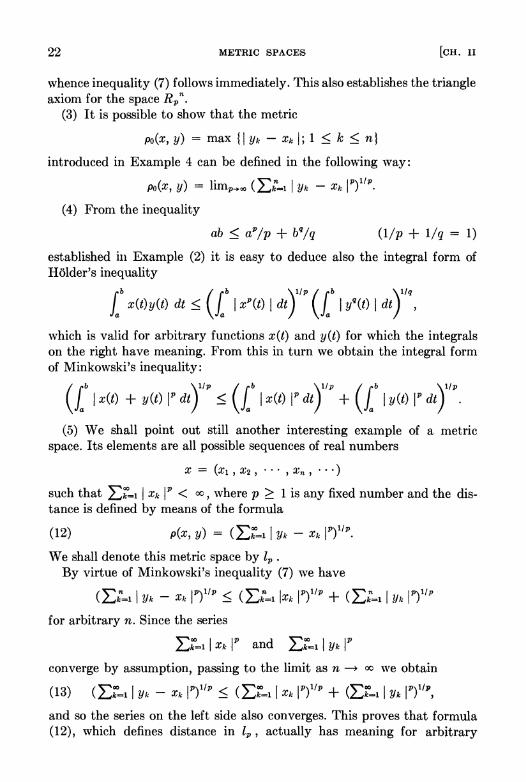
Po(X,y) = max {ly" - xkl; 1 ~ k ~ n}.
The validity of Axioms 1-3 is obvious. In many questions of analysis this space is no less suitable than Euclidean space R".
Examples 3 and 4 show that sometimes it is actually important to have different notations for the set of points of a metric space and for the metric space itself because the same point set can be metrized in various ways.
5. The set era, b] of all continuous real-valued functions defined on the segment [a, b] with distance function
(2) p(f, g) = sup (I g(t) - f(t) I; a ~ t ~ b}

18 METRIC SPACES [CH. II
likewise forms a metric space. Axioms 1-3 can be verified directly. This space plays a very important role in analysis. We shall denote it by the same symbol C[a, b] as the set of points of this space. The space of continuous functions defined on the segment [0, 1] with the metric given above will be denoted simply by C.
G. We denote by l2 the metric space in which the points are all possible f:lequences x = (Xl, X2, ... , X"' ... ) of real numbers which satisfy the condition L:k"-l Xk2 < x: and for which the distance is defined by means of the formula
(:3) p(x, Y) = I L:Z'..1 ClJk - xdl I.
We shall first prove that the function p(x, y) defined in this way always has meaning, i.e. that the series L:k"-l (Yk - xd converges. We have
(4,,) I L::=l (Yk - xk)21l ~ (L:k~l Xk2)! + (L:k'=l Yk2)!
for arbitrary natural number n (see Example 3). N ow let n ~ x:. By hypothesis, the right member of this inequality has
a limit. Thus, the expression on the left is bounded and does not decrease as n ~ oc; consequently, it tends to a limit, i.e. formula (3) has meaning. Replacing x by -x in (4,,) and passing to the limit as n ~ oc, we obtain
(4) {L:k"-l (Yk + xdl 1 ~ (L:Z'..1 Xk2)! + (L:k"-l Yk2)1;
but this is (:'ssentially the triangle axiom. In fact, let
a = (ai, ~, ... , an , ... ),
b = (b l , b2 , ••• , b", ... ) ,
C = (Cl, C2, ••• , C,,' .•• )
be three points in 12 • If we set
then
and, by virtue of (4),
{L:k"-l (Ck - adl l ~ {L:k"-l (bk - adl l + {L:k"-l (Ck - bk)211,
i.e. p(a, c) ~ p(a, b) + p(b, c).
7. Consider, as in Example 5, the totality of all continuous functions on the segment [a, b], but now let the distance be defined by setting
(5) p(x, y) = [{ {x(t) - y(t) 12 dtJ.

§8] DEFINITION AND EXAMPLES OF METRIC SPACES 19
This metric space is denoted by d[a, b] and is called the space of continuous functions with quadratic metric. Here again Axioms 1 and 2 in the definition of a metric space are obvious and the triangle axiom follows immediately from the Schwarz inequality
{ b }2 b b 1 x(t)y(t) dt ~ L x2(t) dt 1 y2(t) dt,
which can be obtained, for instance, from the following easily-verified identity:
{{ x(t)y(t) dtr = { x2(t) dt { y2(t) dt
I1b1b -"2 " " [x(s)y(t) - y(S)X(t)]2 ds dt.
8. Consider the set of all bounded sequences x = (Xl, X2, . .. , xn , ••• )
of real numbers. We obtain the metric space MOO if we set
(6) p(x, y) = sup I Yk - Xk I. The validity of Axioms 1-3 is obvious.
9. The following principle enables us to write down an infinite number of further examples: if R = (X, p) is a metric space and M is an arbitrary subset of X, then M with the same function p(x, y), but now assumed to be defined only for X and yin M, likewise forms a metric space; it is called a subspace of the space R.
(1) In the definition of a metric space we could have limited ourselves to two axioms for p(x, y), namely:
1)
if, and only if, x = 1/;
2)
for arbitrary x, y, z. It follows that
3)
4)
p(x, Y) = 0
p(x, y) ~ p(z, x) + p(z, y)
p(x, y) ~ 0,
p(x, y) = p(y, x)
and consequently Axiom 2 can be written in the form
2') p(x, y) ~ p(x, z) + p(z, y).
(2) The set D n of ordered n-tuples of real numbers with distance
p'p(x, y) = (Lk=l I Yk - Xk IP)l/P (p ~ 1)

20 METRIC SPACES [CH. II
also forms a metric space which we shall denote by Rp n. Here the validity of Axioms 1 and 2 is again obvious. We shall check Axiom 3. Let
.l~ = (XI,:l:'2, ... ,:1",,), lJ = (Yl, Y2 , . . . ,Yn) and Z = (ZI , Z2 , . . . ,Zn)
be points in Rp n. If, as in Example 3, we set
then the inequality
assumes the form
(7) (~::::=I I ak + bk IP)I/p :::; (~:"1 I ak nl/p + (~:"1 I bk IP)I/p. This is the so-called Minkowski inequality. Minkowski's inequality is obvious for p = 1 (since the absolute value of a sum is less than or equal to the sum of the absolute values) and therefore we can restrict ourselves to considering the case p > 1.
In order to prove inequality (7) for p > 1 we shall first establish Holder's inequality:
(8)
where the number q is defined by the condition
(9) lip + l/q = 1.
We note that inequality (8) is homogeneous in the sense that if it is satisfied for any two vectors
x = (XI, X2, ..• ,xn) and y = (Yl, Y2, ... , Yn),
then it is also satisfied for the vectors Xx and p.lJ where X and p. are arbitrary numbers. Therefore it is sufficient to prove inequality (8) for the case when
(10) ~:_I I :l:~k IP = ~:-1 I Yk Iq = 1.
Thus, we must prove that if Condition (10) is satisfied, then
(11) ~:-1 I XkYk I :::; 1.
Consider in the (~, ,,)-plane the curve defined by the equation" = ~P-\ or equivalently by the equation ~ = "q-I (see Fig. 7). It is clear from the figure that for an arbitrary choice of positive values for a and b we have SI + S2 ~ abo If we calculate the areas SI and S2 , we obtain
SI = l a ~P-I d~ = aP /p; S2 = [ "q-I d" = bq/q.

§8)
Thus
DEFINITION AND EXAMPLES OF METRIC SPACES
"l
bl-------f
FIG. 7
ab ~ aP /p + bq/q.
21
Setting a = I Xk I, b = I Uk I and summing with respect to k from 1 to n, we obtain
2::-1 I XkUk I ~ 1,
if we take (9) and (10) into consideration. Inequality (11) and consequently the more general inequality (8) are
thus proved. For p = 2 Holder's inequality (8) becomes the Schwarz inequality (1).
We now proceed to the proof of the Minkowski inequality. Consider the identity
(I a I + I b I)P = (I a I + I b I)P-l I a I + (I a I + I b I)P-l I b I· Setting a = Xk , b = Yk in the above identity and summing with respect to k -from 1 to n, we obtain
2::-1 (I Xk I + I Yk I)P = 2::-1 (I Xk I + I Yk I)P-l I Xk I + 2::"1(1 Xk I + I Yk I)P-l I Yk I·
If we now apply Holder's inequality to each of the two sums on the right of the above equality and take into consideration the fact that (p - 1)q = p, we obtain
2:~1 (I Xk I + I Yk IY' ~ 12::-1 (I Xl: I + I Uk I)P}l/q{(2:k'!..ll Xk IP)l/p + (2::-11 Yk IP/lp).
Dividing both sides of this inequality by
{ 2::=1 (I Xk I + I 'Uk I)P}I/Q,
we obtain
{2:':-1 (I Xk I + I Yk ly}l/p ~ (2:k'!..l I Xk IP)l/p + (2::=1 I Yk IP)l/p,
22 METRIC SPACES [CH. II
whence inequality (7) follows immediately. This also establishes the triangle axiom for the space R/.
(3) It is possible to show that the metric
Po(x, y) = max {I Yk - Xk I; 1 :::; k :::; n}
introduced in Example 4 can be defined in the following way:
Po(x, y) = limlHoo (2::-1 1 Yk - Xk Ilj1/1'.
(4) From the inequality
(lip + l/q = 1)
established in Example (2) it is easy to deduce also the integral form of Holder's inequality
lb (lb )1/1' (lb )l/q a X(t)y(t) dt:::; a 1 XP(t) 1 dt a 1 yq(t) 1 dt ,
which is valid for arbitrary functions x(t) and yet) for which the integrals on the right have meaning. From this in turn we obtain the integral form of Minkowski's inequality:
(lb )1/1' (lb )l/P (lb )1/1' a 1 x(t) + yet) 11' dt :::; a 1 x(t) 11' dt + a 1 yet) 11' dt .
(5) We shall point out still another interesting example of a metric space. Its elements are all possible sequences of real numbers
x = (Xl, X2, •• , , x n , ••• )
such that 2:~1 1 Xk 11' < <Xl, where p ~ 1 is any fixed number and the distance is defined by means of the formula
(12) p(x, y) = (2::'..11 Yk - Xk 11')1/1'.
We shall denote this metric space by l1' • By virtue of Minkowski's inequality (7) we have
(2::-11 Yk - Xk JP)l/1' :::; (2::-1 IXk 11')1/1' + (2::=11 Yk Ilj1/p
for arbitrary n. Since the series
2::'=1 1 Xk 11' and 2:~1 1 Yk 11' converge by assumption, passing to the limit as n - <Xl we obtain
(13) (2::'1 1 Yk - Xk 11')1/1' :::; (2::'=1 1 Xk 11')1/1' + <2:k...1 1 Yk 11')1/1',
and so the series on the left side also converges. This proves that formula (12), which defines distance in l1" actually has meaning for arbitrary

§9] CONVERGENCE OF SEQUENCES. LIMIT POINTS 23
x, yElp. At the same time inequality (13) shows that the triangle axiom is satisfied in lp . The remaining axioms are obvious.
§9. Convergence of sequences. Limit points
In §§9-U we shall establish some fundamental concepts which we shall frequently use in the sequel.
An open sphere S(xo, r) in the metric space R is the set of all points x E R which satisfy the condition p(x, xo) < r. The fixed point Xo is called the center and the number r is called the radius of this sphere.
A closed sphere S[xo, r] is the set of all points x E R which satisfy the condition p(x, xo) ~ r.
An E-neighborhood of the point x, denoted by the symbol O(x, E), is an open sphere of radius E and center Xo .
A point x is called a contact point of the set M if every neighborhood of x contains at least one point of M. The set of all contact points of the set M is denoted by [M] and is called the closure of M. Since every point belonging to M is obviously a contact point of M (each point is contained in every one of its neighborhoods), every set is contained in its closure: M ~ [M].
THEOREM 1. The closure of the closure of M is equal to the closure of M:
[[M]] = [M].
Proof. Let x E [[Mll. Then an arbitrary E-neighborhood O(x, E) of x contains a point Xl E [M]. Setting E - p(x, Xl) = EI, we consider the sphere O(XI, EI). This sphere lies entirely in the interior of O(x, E). In fact, if z E O(XI, EI), then p(z, Xl) < EI ; and since p(x, Xl) = E - EI, then, by the triangle axiom p(z, x) ~ EI + (E - EI) = E, i.e. z E O(x, E). Since Xl E [M], O(x, EI) contains a point X2 E M. But then X2 E O(x, E). Since O(x, E) is an arbitrary neighborhood of the point x, we have X E [M]. This completes the proof of the theorem.
The validity of the following assertion is obvious. THEOREM 2. If MI ~ M, then [MI] ~ [M]. THEOREM 3. The closure of a sum is equal to the sum of the closures:
[MI U M 2] = [MI] U [M2].
Proof. Let X E [MI U M2], i.e. let an arbitrary neighborhood O(x, E) contain the point y E MI U M2 • If it were true that X EE [MI] and X EE [M2],
we could find a neighborhood O(x, EI) which does not contain points of M I and a neighborhood O(x, E2) which does not contain points of M 2 • But then the neighborhood O(x, E), where E = min (EI, E2), would not contain points of MI U M 2 • From the contradiction thus obtained it follows that X is contained in at least one of the sets [MI] and [M2], i.e.
[MI U M 2] ~ [MI ] U [M2].

24 METRIC SPACEI'; [Clf. II
Since 1\111 ~ 1\111 U 1112 and 1112 C Ml U M2, the converse inclusion follows from Theorem 2.
The point x is called a limit point of the set M if an arbitrary neighborhood of x contains an infinite number of points of M.
A limit point of the set 111 can eit.her belong to jll or not. For example, if .ll is the set of rational numbers in the closed interval [0, 1], then every point of this interval is a limit point of M.
A point x belonging to the set jj[ is said to be an isolated point of t.hi:,; ~t if x has a neighborhood O(x, E) which does not contain any points of M different from x.
TUEOREM 4. Every contact point oj' the set !Ii is either a limit point of the set 111 or an isolated point of M.
Proof. Let x be a contact point of t.he !:let M. This means that every neighborhood O(:c, E) of x contains at least one point belonging to Ill. Two cases are possible:
1) Every neighborhood of the point :r contains an infiuite number of points of the set lIf. In this case, x is a limit point of lIf.
2) We can find a neighborhood O(x, E) of x which contains only a finite number of points of 111. In this case, x will be an isolated point of the set lIf. In fact, let Xl , J'2, ..• , Xk be the points of lrI which are dist.inct from x and which are contained in the neighborhood O(x, E). Further, let Eo be the least of the positive numbers p(x, x;), i = 1, 2, ... , k. Then the neighborhood O(x, EO) obviously does not contain any point of ill distinct from x. The point x itself in this case must necessarily belong to ill since othenvise O(x, Eo) in general would not contain a single point of lvI, i.e. x would not be a contact point of the set lIf. This completes the proof of the theorem.
Thus, the set [111] consists in general of points of three types: 1) Isolated points of the set 111; 2) Limit points of the set 111 which belong to M; 3) Limit points of the set 111 which do not belong to M.
[111] is obtained by adding to jj[ all its limit points. Let J'1 , :/"2, ••• be a sequence of points in the metric space R. We say
that this sequence converges to the point x if every neighborhood O(x, E) contains all points Xn starting with some one of them (i.e. if for every E > 0 we can find a natural number N. such that O(x, E) contains all points .f" with n > N,). The point :/.' is said to he the limit of the sequence I x" I.
This definition ran obviou!:lly be formulated in the following form: the :,;cquenre I:r" 1 converges to :l: if lim" ... ", p(:l~, Xn) = O.
The following assertions follow dit'ectly from the definition of limit: 1) 110 sequence can have two distinct limits; 2) if the sequence IX n 1 l'onvergeH to the point x then every subsequence of I :1:" I l'Ol1\"erges to the same point :1'.
The following th('orem establishes the close connection hetween the

§9] CONVERGENCE OF SEQUENCES. LIMIT POIl';""TR 25
concepts of contact point and limit. point on the one hand and the concept of limit on the other.
THEOREM 5. A necessary and suffteient condition that the point x be a contact point of the set M is that there exist a sequence {x" I of points of the set M which converges to Xj a necessary and sufficient condition that the point x be a limit point of M is that there exist a sequence of distinct points of the set M which converges to x.
Proof. Necessity. If x is a contact point of the set M, then every neighborhood O(x, lin) contains at least one point Xn of M. These points form a sequence which converges to x. If the point x is a limit point of M, every neighborhood O(x, lin) contains a point x" E M which is distinct from all the xi(i < n) (since the number of such points is finite). The points x" are distinct and form a sequence which converges to x.
Sufficiency is obvious. Let A and B be two sets in the metric space R. The set A is said to be
dense in B if [A] :::> B. In particular, the set A is said to be everywhere dense in R if its closure [A] coincides with the entire space R. For example, the Ret of rational numbers is everywhere dense on the real line.
EXAMPLES OF SPACES CONTAINING AN EVERYWHERE DENSE DENUMERABLE SET. (They are sometimes called "separable." For another definition of such spaces in terms of the concept of basis see §10, Theorem 4.) We shall consider the very same examples which were pointed out in §8.
1. The space described in Example 1, §8, is separable if, and only if, it consists of a denumerable number of points. This follows directly from the fact that in this space [M] = M for an arbitrary set M.
All spaces enumerated in Examples 2-7, §8, are separable. We shall indicate a denumerable everywhere dense set in each of them and leave the details of the proof to the reader.
2. Rational points. ~. The set of all vectors with rational coordinates. 4. The set of all vectors with rational coordinates. 5. The set of all polynomials with rational coefficients. 6. The set of all sequences in each of which all terms are rational and
only a finite (but arbitrary) number of terms is distinct from zero. 7. The set of all polynomials with rational coefficients. The space of bounded sequences (Example 8, §8) is not separable. In
fact, let us consider all possible sequences consisting of zeros and ones. They form a set with cardinal number that of the continuum (since each of them can be put into correspondence with the dyadic development of some real number which is contained in the interval [0, 1]). The distance between two such distinct points defined by formula (6), §8, is 1. We surround each of these points with a sphere of radius !. These spheres do not intersect. If

26 METRIC SPACES [CH. II
some set is everywhere dense in the space under consideration, then each of the indicated spheres should contain at least one point of this set and consequently it cannot be denumerable.
(1) Let A be an arbitrary set in the metric space R and let x be a point in R. The distance from the point x to the set A is defined by the number
p(A, x) = inf {p(a, x); a E AI.
If x E A, then p(A, x) = 0; but the fact that p(A, x) = 0 does not imply that x EA. From the definition of contact point it follows immediately that p(A, x) = 0 if, and only if, x is a contact point of the set A.
Thus, the closure [A] of the set A can be defined as the totality of all those points whose distance from the set A is zero.
(2) We can define the distance between two sets analogously. If A and B are two sets in R, then
p(A, B) = inf {p(a, b); a E A, b E BI.
If A n B ¢ 8, then p(A, B) = 0; the converse is not true in general. (3) If A is a set in the metric space R then the totality A' of its limit
points is called its derived set. Although the application to [M] once more of the operation of closure
always results again in [M], the equality (M'Y = M' does not hold in general. In fact, if we take, for example, the set A of points of the form lin on the real line, then its derived set A' consists of the single point 0, but the set A" = (A')' will already be the void set. If we consider on the real line the set B of all points of the form lin + 1/(nm) (n, m = 1, 2, ... ), then B' = A U A', B" is the point 0, and Bill is the void set.
§10. Open and closed sets
In this section we shall consider the more important types of sets in a metric space; these are the open and closed sets.
A set M in a metric space R is said to be closed if it coincides with its closure: [M] = M. In other words, a set is said to be closed if it contains all its limit points.
By Theorem 1, §9, the closure of an arbitrary set M is a closed set. Theorem 2, §9, implies that [M] is the smallest closed set which contains M.
EXAMPLES. 1. An arbitrary closed interval [a, b] on the real line is a closed set.
2. The closed sphere is a closed set. In particular, in the space era, b] the set of functions satisfying the condition I f I :::;; K is closed.
3. The set of functions satisfying the condition I f I < K (open sphere) is not closed; its closure is the set of functions satisfying the condition If I :::;; K.

§1O] OPEN AND CLOSED SETS 27
4. Whatever the metric space R, the void set and the whole space R are closed sets.
5. Every set consisting of a finite number of points is closed. The fundamental properties of closed sets can be formulated in the form
of the following theorem. THEOREM 1. The intersection of an arbitrary number and the sum of an
arbitrary finite .number of closed sets are closed sets. Proof. Let F = naF a, where the Fa are closed sets. Further, let x be a
limit point of the set F. This means that an arbitrary neighborhood O(x, E) of x contains an infinite number of points of F. But then O(x, E) contains an infinite number of points of each Fa and consequently, since all the Fa are closed, the point x belongs to each Fa; thus, x E F = naF a, i.e. F is closed.
Now let F be the sum of a finite number of closed sets: F = U~_l F i ,
and let x be a point not belonging to F. We shall show that x cannot be a limit point of F. In fact, x does not belong to any of the closed sets Fi and consequently it is not a limit point of any of them. Therefore for every i we can find a neighborhood O(x, Ei) of the point x which does not contain more than a finite number of points of F i . If we take the smallest of the neighborhoods O(x, El), ... , O(X, En), we obtain a neighborhood O(x, E) of the point x which does not contain more than a finite number of points of F.
Thus, if the point x does not belong to F, it cannot be a limit point of F, i.e. F is closed. This completes the proof of the theorem.
The point x is said to be an interior point of the set M if there exists a neighborhood O(x, E) of the point x which is contained entirely in M.
A set all of whose points are interior points is said to be an open set. EXAMPLES. 6. The interval (a, b) of the real line Dl is an open set; in fact,
if a < a < b, then O(a, E), where E = min (a - a, b - a), is contained entirely in the interval (a, b).
7. The open sphere Sea, r) in an arbitrary metric space R is an open set. In fact, if x E Sea, r), then pea, x) < r. We set E = r - pea, x). Then sex, E) c Sea, 1').
8. The set of continuous fUllctions satisfying the condition I f I < K, where K is an arbitrary number, is an open subset of the space era, b].
THEOREM 2. A necessary and su.tficient condition that the set M be open is that its complement R "" M with respect to the whole space R be closed.
Proof. If M is open, then each point x E M has a neighborhood which belongs entirely to M, i.e. which does not have a single point in common with R "" M. Thus, no point which does not belong to R "" M can be a contact point of R "" M, i.e. R "" M is closed. Conversely, if R "" M is closed, an arbitrary point of M has a neighborhood which lies entirely in M, i.e. M is open.

28 ME'l'RH' 81'ACI<;S [CH. 11
Rinc:e the \'oid RCt alld the whole :spaN' R are dosed and are at the same time complements of eueh other, the theorem proved abO\'e implies the following corollary.
COROLl,AHY. The \'oid Ret and whole ~pa('e R are open sets. The following important theorem whirh if> the dual of Theorem 1 follows
from Theorem ] and the prineiple of duality established ill § 1 (the int('rsection of ('omplements equals the eomplement of the sums, the sum of thf' eomplemelltR equalK the eomplement of the intersections).
THIWREl\I ]'. The sum of an ar~itrary number and the intersection of all arbitrary finite number of open sets are open sets.
A family {G a } of opcn sets in R is ('alled a basis in R if ewry open :set in R can be represented as the sum of a (finite or infinite) number of sets belonging to this family.
To cheek whether or not a gi\'cll family of open sets is a basis we find the following eriterion useful.
THTWUEl\I :3 . .'1 necessary and sUfficient condition that a system of open scts I G a} be a basis in R is that for ew'y opcn set G and for el'cry point .1: E G a set Ga can be f01tnd in this slJstem such that x c: Ga C G.
Proof. If {G a} is a basis, then every open set G is a sum of G a's: G = U; Ga ; , and consequent.ly every point x in G belongs to some G", contained in G. Conversely, if the condition of the theorem is fulfilled, then {Ga} is a basis. 1n fact, let G be an arbitrary open set. For each point ;1: E G we can find some Ga(x) such that:t: E G", c G. The sum of these Ga(x) OWl' all .1: E G equals G.
With the aid of this criterion it is easy to establish that in every metrie space the family of all open spheres forms a basis. The family of all spheres with rational radii also forms a basis. On the real line a basis is formed, for example, by the family of all rational intervals (Le. intervals with rational endpoints).
We shall say that a set is countable if it is either finite or denumerable. R is said to be a space with countable basis or to satisfy the second axiom
of countability if there is at least pne basis in R consisting of a countable number of elements.
THEOREM 4. A necessary and sufficient condition that R be a space with countable basis is that there exist in R an everywhere dense countable set. (A finite everywhere dense set occurs only in spaces consisting of a finite set of points.)
Proof. Necessity. Let R have a countable basis {Gn }. Choose from each Gn.an arbitrary point Xn • The set {xn } obtained in this manner is everywhere dense in R. In fact, let x be an arbitrary point in R and let O(x, e) be a neighborhood of .r. According to Theorem 3, a set Gn can be found such that X' E Gn C O(x, e). Since Gn contains at least one of the points of

§10] OPEN AND CLOSED SETR 29
t.he set Ix,,}, any neighborhood 0(:1', e) of an arbitrary point .1' C: R eontain~ at least one point from f Xn I and this mean~ that h'" I is cwrrwherC' denRe in R.
Su:lficiency. If l.tn I iR a countable eyerywhcrc dense :-l'i in R, thell th(' family of sphere~ S(a.·n , I/k) forms a eoulltable basi:; ill H. In fact, the s!:'t of all these spheres is countahle (i1eing the sum of a ('onntable family of ('ountable sets). Further, let G he an arbitrary open set and let ;1' be any point in G. By t.he definition of an open set an m > 0 can be found such that the sphere S(.r, 11m) lies !:'ntirely in G. We now sel!:'ct a point .1'"o
from the set {.r,,) such that p(.I:, J:"o) < 1/:3111. Then the sphere S(x"o ,l 12m) contains the point .1' and is ('ontained in Sex, lim) and (·onsequent.ly ill G also. By virtue of Theorem :3 it follows from t,his that the spheres S(xn , 11k) form a basis in H.
By virtue of this theorem, the examples introduced above (§ 9) of separable spaces are at. the 8am!:' t.ime examples of spaces with count.able basis.
We say that a system of sets ...11 a is a covering of the space R if UM a = H. A covering consisting of op!:'n (dos!:'d) s!:'ts ,,"ill be called an open (clo.~('d)
covering. THEoHEl\I 5. If If is a metric spac(' with countable llasis, then we can select
(l countable covering from each of its open co~·erings. Proof. Let lOa I be an al'bitl'ary open covering of R. Thus, <"'ery point
;t' E R is contained in some Oa . Let {G" I be a countablt· basis in R. Then for every x E R there exists a
Gn(x) E {G"I atld an a such that J.' EGner) c Oa. The family of set.s Gn(x) selected in this way is countable and covers R. If we ehoose for each of the Gn(.t) one of the sets Oa containing it., we obtain a countable sub('overing of the covering {O a I.
It was already indi('ated ahove that t.he void set and the entire space II are simultaneously opeu and closed. A spa('e in which there are no other sets whieh are ~il11ultaneously open and dosed is said to be connected. The real line R1 is one of th(' :;implest examples of a connected metric spacc. But if we remow a fillite set of points (for example, one point) from R\ the remaining :;pace is no longer connected. The simplest example of a Rpace whieh is not ('onnected iR the space consisting of t.wo points which are at an arbitrary distance from one anoth!:'r.
(1) Let 11h b(' the set. of all functionsf in era, b] which satisfy a so-called Lipschitz ('ondition
IJ(t1) - f(t2) 1 ~ K 1 t4 - t21,
where K is a constant. The set lHk is closed. It coincides with the closure of the set of all differentiable functions which are such that I.f'(t) 1 ~ K.

30 METRIC SPACES [ell. II
(2) The set M = UkM k of all functions each of which satisfies a Lipschitz condition for some K is not closed. Since JJ1 contains the set of all polynomials, its closure is the entire space era, b].
(3) Let distance be defined in the space X in two different ways, i.e. let there be given two distinct metrics Pl(X, y) and P2(X, V). The metrics PI and P2 are said to be equivalent if there exist two positive constants a and b such that a < [PI (x, y) / P2(X, y)] < b for all x ~ y in R. If an arbitrary set M C X is closed (open) in the sense of the metric PI , then it is closed (open) in the sense of an arbitrary metric P2 which is equivalent to PI .
(4) A number of important definitions and assertions concerning metric spaces (for example, the definition of connectedness) do not make use of the concept of metric itself but only of the concept of open (closed) set, or, what is essentially the same, the concept of neighborhood. In particular, in many questions the metric introduced in a metric space can be replaced by any other metric which is equivalent to the initial metric. This point of view leads naturally to the concept of topological space, which is a generalization of metric space.
A topological space is a set T of elements of an arbitrary nature (called points of this space) some subsets of which are labeled open sets. In this connection we assume that the following axioms are fulfilled:
1. T and the void set are open; 2. The sum of an arbitrary (finite or infinite) number and the inter
section of an arbitrary finite number of open sets are open. The sets T ~ G, the complements of the open sets G with respect to T,
are said to be closed. Axioms 1 and 2 imply the following two assertions. 1'. The void set and T are closed; 2'. The intersection of an arbitrary (finite or infinite) number and the
sum of an arbitrary finite number of closed sets are closed. A neighborhood of the point x E T is any open set containing x. In a natural manner we introduce the concepts of contact point, limit
point, and closure: x E T is said to be a contact point of the set M if every neighborhood of the point x contains at least one point of M; x is said to be a limit point of the set M if every neighborhood of the point x contains an infinite number of points of M. The totality of all contact points of the set M is called the closure [M] of the set M.
It can easily be shown that closed sets (defined as the complements of open sets), and only closed sets, satisfy the condition [M] = M. As also in the case of a metric space [M] is the smallest closed set containing M.
Similarly, as a metric space is the pair: set of points and a metric, so a topological space is the pair: set of points and a topology defined in this space. To introduce a topology into T means to indicate in T those subsets which are to be considered open in T.

§1l] OPEN AND CLOSED SETS ON THE REAL LINE 31
EXAMPLES. (4-a) By virtue of Theorem l' open sets in a metric space satisfy Conditions 1 and 2 in the definition of a topological space. Thus, every metric space can be considered as a topological space.
(4-b) Let T consist of two points a and b and let the open sets in T be T, the void set, and the set consisting of the single point b. Axioms 1 and 2 are fulfilled. The closed sets are T, the void set, and the set consisting of the single point a. The closure of the set consisting of the point b is all of T.
(5) A topological space T is said to be metrizable if a metric can be introduced into the set T so that the sets which are open in the sense of this metric coincide with the open sets of the initial topological space. The space (4-b) is an example of a topological space which cannot be metrized.
(6) Although many fundamental concepts carryover from metric spaces to topological spaces defined in (4), this concept turns out to be too general in a number of cases. An important class of topological spaces consists of those spaces which satisfy, in addition to Axioms 1 and 2, the Hausdorff separation axiom:
3. Any two distinct points x and y of the space T have disjoint neighborhoods.
A topological space satisfying this axiom is called a Hausdorff space. Clearly, every metric space is a Hausdorff space. The space pointed out in Example (4-b) does not satisfy the Hausdorff axiom.
§11. Open and closed sets on the real line
The structure of open and closed sets in an arbitrary metric space can be very complicated. We shall now consider the simplest special case, namely that of open and closed sets on the real line. In this case their complete description does not present much of a problem and is given by the following theorem.
THEoREM 1. Every open set on the real line is the sum of a countable number of disjoint intervals.
Proof. [We shall also include sets of the form (- co, co), (0:, co), (- co, (j) as intervals.] Let G be an open set and let x E G. Then by the definition of an open set we can find some interval I which contains the point x and belongs entirely to the set G. This interval can always be chosen so that its endpoints are rational. Having taken for every point x EGa corresponding interval I, we obtain a covering of the set G by means of a denumerable system of intervals (this system is denumerable because the set of all intervals with rational endpoints is denumerable). Furthermore, we shall say that the intervals I' and I" (from the same covering) belong to one class if there exists a finite chain of intervals:
I' = II, 12 , ••• , In = I"

32 METRIC SPACES [CH. II
(belonging to our covering) such that h intersects Ik+l (1 ~ k ~ n - 1). It is clear that there will be a countable number of such classes. Further, the union of all the intervals which belong to the same class obviously again forms an interval U of the same type, and intervals corresponding to distinct classes do not intersect. This completes the proof of the theorem.
Since closed sets are the complements of open sets, it follows that every closed set on the real line is obtained by removing a finite or denumerable number of open intervals on the real line.
The simplest examples of closed sets are segments, individual points, and the sum of a finite number of such sets. We shall now consider a more complicated example of a closed set on the real line, the so-called Cantor set.
Let Fo be the closed interval [0, 1]. We remove the open interval (1, I) from Fo and denote the remaining closed set by Fl. Then we remove the open intervals (t, }) and (t, t) from Fl and denote the remaining closed set (consisting of four closed intervals) by F2 . From each of these four intervals we remove the middle interval of length (1)3, and so forth. If we continue this process, we obtain a decreasing sequence of closed sets F n • We set F = n:-o F n ; F is a closed set (since it is the intersection of the closed sets Fn). It is obtained from the closed interval [0, 1] by removing a denumerable number of open intervals. Let us consider the structure of the set F. The points
(1) ° 1 ~ 3 ~ 2 7 8 ••• , ,11"1 3, 11"1 11", 11", 11",
which are the endpoints of the deleted intervals obviously belong to F. However, the set F is not exhausted by these points. In fact, those points of the closed interval [0, 1] which belong to the set F can be characterized in the following manner. We shall write each of the numbers x, ° ~ x ~ 1, in the triadic system:
x = at/3 + a,/32 + ... + an/3n + ... , where the numbers an can assume the values 0, 1, and 2. As in the case of the ordinary decimal expansion, some numbers allow two different developments. For example,
i = t + (t)2 + ... + mn + ... = i + (1)2 + (1)3 + ... + (I)n + .... It is easily verified that the set F contains those, and only those, numbers
x, ° ~ x ~ 1, which can be written in at least one way in the form of a triadic fraction such that the number 1 does not appear in the sequence al , a, , . .. ,an , . .. . Thus, to each point x E F we can assign the sequence
(2)

§12] CONTINUOUS MAPPINGS. HOMEOMORPHISM. ISOMETRY
where an is 0 or 2. The set of all such sequences forms a set having the power of the continuum. 'Ve can convince ourselves of this by assigning to each sequence (2) the sequence
(2') b1 , b2 , ••• , bn , ••• ,
where bn = 0 if an = 0 and bn = 1 if an = 2. The sequence (2') can be considered as the development of a real number y, 0 ~ y ~ 1, in the form of a dyadic fraction. We thus obtain a mapping of the set F onto the entire closed interval [0, 1]. This implies that F has the cardinal number of the continuum. [The correspondence established between F and the closed interval [0, 1] is single-valued but it is not one-to-one (because of the fact that the same number can sometimes be formed from distinct fractions). This implies that F has cardinal number not less than the cardinal number of the continuum. But F is a subset of the closed interval [0, 1] and consequently its cardinal number cannot be greater than that of the continuum. (See §5.)] Since the set of points (1) is denumerable, these points cannot exhaust all of F.
EXERCISE. Prove directly that the point t belongs to the set F although it is not an endpoint of a single one of the intervals deleted. Hint: The point t divides the closed interval [0, 1] in the ratio 1: 3. The closed interval [0, t] which remains after the first deletion is also divided in the ratio 1::3 by the point t, and so on.
The points (1) are said to be points of the first type of the set F and the remaining points are said to be points of the second type.
EXERCISE. Prove that the points of the first type for111 an eYery,,-here dense set in F.
'Ve have shown that the set F has the cardinal number of the continuum, i.e. that it contains as many points as the entire closed interval [0, 1].
It is interesting to compare this fact with the following result: the sum of the lengths of all the deleted intelTals is t + i + -l'r + ... , i.e. exactly 1 !
§12. Continuous mappings. Homeomorphism. Isometry
Let R = (X, p) and R' = (1', p') be two metric spaces. The mapping f of the space R into R' is said to be continuolls at the point Xo E R if for arbitrary E > 0 a (j > 0 can be found such that
p'[f(x), f(.l·o)] < E
for all :r such that
pC:!', :t·o) < (j.
In other ,Yords, the mappingf is continuous at the point .l'o if an arbitrary

34 METRIC SPACES [CH. II
neighborhood O(j(xo), e) of the point f(xo) contains a neighborhood O(xo , 8) of the point Xo whose image is contained in the interior of O(f(xo), e).
A mapping f is said to be continuous if it is continuous at each point of the space R.
If R' is the real line, then a continuous mapping of R into R' is called a continuous function on R.
As in the case of the mapping of arbitrary sets we shall say that f is a mapping of R onto R' if every element y E R' has at least one inverse image.
In analysis, together with the definition of the continuity of a function "in terms of neighborhoods", the definition of continuity "in terms of sequences", which is equivalent to it, is widely used. The situation is analogous also in the case of continuous mappings of arbitrary metric spaces.
THEOREM 1. A necessary and sufficient condition that the mapping f be continuous at the point x is that for every sequence {xn} which converges to x the corresponding sequence {f(xn)} converge to y = f(x).
Proof. The necessity is obvious. We shall prove the sufficiency of this condition. If the mapping f is not continuous at the point x, there exists a neighborhood O(y, e) of the point y = f(x) such that an arbitrary O(x, 8) contains points whose images do not belong to O(y, e). Setting 8n = lin (n = 1, 2, ... ), we select in each sphere O(x, lin) a point Xn such that f(xn) (£ O(y, e). Then Xn ~ x but the sequence {f(xn)} does not converge to f(x), i.e. the condition of the theorem is not satisfied, which was to be proved.
THEOREM 2. A necessary and sufficient condition that the mapping f of the space R onto R' be continuous is that the inverse image of each closed set in R' be closed.
Proof. Necessity. Let M !:: R be the complete inverse image of the closed set M' ~ R' . We shall prove that M is closed. If x E [M], there exists a sequence {xn } of points in M which oonverges to x. But then, by Theorem 1, the sequence {f(xn )} converges to f(x). Since f(xn ) E M' and M' is closed, we have f(x) E M'; consequently x E M, which was to be proved.
SUfficiency. Let x be an arbitrary point in R, y = f(x), and let O(y, e) be an arbitrary neighborhood of y. The set R' "" O(y, e) is closed (since it is the complement of an open set). By assumption, F = rl(R' "" O(y, e)) is closed, and moreover, x (£ F. Thus, R "" F is open and x E R "" F; consequently, there is a neighborhood O(x, 8) of the point x which is contained in R "" F. If z E O(x, 8), then fez) E O(y, e), i.e. f is continuous, which was to be proved.
REMARK. The image of a closed set under a continuous mapping is not necessarily closed as is shown by the following example: map the half-open

§12] CONTINUOUS MAPPINGS. HOMEOMORPHISM. ISOMETRY
o J. a
FIG. 8
35
interval [0, 1) onto a circle of the same length. The set [!, 1) which is closed in [0, 1), goes over under this mapping into a set which is not closed (see Fig. 8).
Since in the case of a mapping "onto" the inverse image of the complement equals the complement of the inverse image, the following theorem which is the dual of Theorem 2 is valid.
THEOREM 2'. A necessary and sufficient condition that the mapping f of the space R onto R' be continuous is that the inverse image of each open set in R' be open.
The following theorem which is the analogue of the well-known theorem from analysis on the continuity of a composite function is valid for continuous mappings.
THEOREM 3. If R, R', R" are metric spaces and f and rp are continuous mappings of R into R' and R' into R", respectively, then the mapping z rp(f(x)) of the space R into R" is continuous.
The proof is carried out exactly as for real-valued functions. The mapping f is said to be a homeomorphism if it is one-to-one and
bicontinuous (i.e. both f and the inverse mapping r 1 are continuous). The spaces Rand R' are said to be homeomorphic if a homeomorphic
correspondence can be established between them. It is easy to see that two arbitrary intervals are homeomorphic, that an
arbitrary open interval is homeomorphic to R\ and so forth. It follows from Theorems 2 and 2' of this section that a necessary and
sufficient condition that a one-to-one mapping be a homeomorphism is that the closed (open) sets correspond to closed (open) sets.
This implies that a necessary and sufficient condition that a one-to-one mapping rp be a homeomorphism is that the equality
hold for arbitrary M. (This follows from the fact that [M] is the intersection of all closed sets which contain M, i.e. it is the minimal closed set which contains M.)
EXAMPLE. Consider the spaces R n = (D", p) and Ron = (Dn, po) (see §8,

36 METRIC SPACES [CH. II
Examples 3 and 4). The following inequalities hold for the mapping which assigns to an element in Rn with coordinates Xl, X2, ..• , Xn the element in Ro n with the same coordinates:
po(x, y) ~ p(x, y) ~ nipo(x, y).
Consequently an arbitrary e-neighborhood of the point x of the space R n
contains a 8-neighborhood of the same point X considered as an element of the space Ron, and conversely. It follows from this that our mapping of R n onto Ron is a homeomorphism.
An important special case of a homeomorphism is an isometric mapping. We say that a one-to-one mapping y = f(x) of a metric space R onto a
metric space R' is isometric if
P(Xl, X2) = p'[f(Xl) , f(X2)]
for arbitrary Xl , X2 E R. The spaces Rand R' themselves, between which an isometric correspondence can be established, are said to be isometric.
The isometry of two spaces Rand R' means that the metric relations between their elements are the same and that they can differ only in the nature of their elements, which is unessential. In the sequel we shall consider two isometric spaces simply as identical.
(1) The concept of continuity of a mapping can be defined not only for metric but also for arbitrary topological spaces. The mapping f of the topological space T into the topological space T' is said to be continuous at the point :1'0 if for arbitrary neighborhood O(yo) of the point Yo = f(a'o) there exists a neighborhood O(xo) of the point Xo such that f(O(xo)) c O(yo).
Theorems 2 and 3 carryover automatically to continuous mappings of topological spaces.
§13. Complete metric spaces
From the yery beginning of our study of mathematical analysis we are convinced of the important role in analysis that is played by the property of completeness of the real line, i.e. the fact that every fundamental sequence of real numbers converges to some limit. The real line represents the simplest example. of the so-called complete metric spaces whose basic properties we shall consider in this section.
We shall call a sequence {x,,} of points of a metric space R a fundamental sequence if it satisfies the Cauchy criterion, i.e. if for arbitrary e > 0 there e.rists an N. such that p(x"" .f",,) < efor all n' ~ N., n" ~ N •.
It follows directly from the triangle axiom that eyery convergent sequence is fundamental. In fact, if {.t',,} com'erges to x, then for giyen e > 0 it is possible to find a natural number N. such that p(:!". , x) < e/2 for all n ~ N •. Then p(xn' , a'",,) ~ p(a'n' , x) + P(Xn" , x) < e for arbitrary n' ~ N. and nil ~ N •.

§13] COMPLETE METRIC SPACER 37
DEFINITION 1. If every fundamental sequence in the space R converges to an element in R, R is said to be complete.
EXAMPLES. All the spaces considered in §8, with the exception of the one given in Example 7, are complete. In fact:
1. In the space consisting of isolated points (Example 1, §8) only those sequences in which there is a repetition of some point, beginning with some index, are fundamental. Clearly, every such sequence converges, i.e. this space is complete.
2. The completeness of the space Rl of real numbers is known from analysis.
3. The completeness of the Euclidean space R" follows directly from the completeness of Rl. In fact, let {xd be a fundamental sequence; this means that for every E > 0 an N = N. can be found such that
"'" «k) (k»)2 < 2 .£...k-l Xp - Xq E
for all p, q greater than N. Then for each k = 1, 2, ... , n
I Xp(k) - Xq(k) I < E
for all p, q > N, i.e. {Xp (4')} is a fundamental sequence of real numbers. We set
X(k) = limp-o .. xp (k),
and
Then it is obvious that
lim" ..... x" = x.
4. The completeness of the space Ron is proved in an exactly analogous manner.
5. We shall prove the completeness of the space C[a, b]. Let {Xn(t)} be a fundamental sequence in C[a, b]. This means that for each E > 0 there exists an N such that I x,,(t) - Xm(t) I < E for n, m > N and all t, a ~ t ~ b. This implies that the sequence {x,,(t)} converges uniformly and that its limit is a continuous function x(t), where
I xn(t) - x(t) I < E
for all t and for all n larger than some N; this means that {Xn(t)} converges to x(t) in the sense of the metric of the space C[a, b].
6. The space l2 . Let {x (n)}, where
be a fundamental sequence in l2 .

38 METRIC SPACES [ClIo II
For arbitrary E > 0 an N can be found such that
(1) 2( (n) (m») ,",00 «n) (m»)2 < E for N p x ,X = L.tk=l Xk - Xk n, m > . It follows from this that for arbitrary k
(Xk (n) _ :/"k (m»)2 < E,
i.e. for each k the sequence of real numbers {Xk (n) } converges. Set lim,,->oo Xk (n) = Xk. Denote the sequence (Xl, X2, ••• , Xn , ••• ) by X. We must show that
To this end we shall write inequality (1) in the form
E~l (Xk (n) - Xk (m»)2
= E!.l (Xk (n) - Xk (m»)2 + E~M+I (Xk (n) - Xk (m»)2 < E
(M arbitrary). Since each of these two sums is nonnegative, each of them is less than E. Consequently
E~l (Xk (n) - Xk (m»)2 < E.
If we fix m in this inequality and pass to the limit as n ~ 00, we obtain
E!.l (Xk - Xk (m»)2 ~ E.
Since this inequality is valid for arbitrary M, we can pass to the limit as M ~ 00. We then obtain
,",00 ( (m»)2 < L.tk=l Xk - Xk _ E.
The inequality thus obtained and the convergence of the series E~=l Xk (m)2 imply that the series E~-l Xk2 converges; consequently x is an element in l2. Further, since E is arbitrarily small, this inequality means that
1· «m») l' {,",oo ( (ml)2}! 0 . lmm ... oo p X ,X = lmm ... oo L.tk=l Xk - Xk =, • (n) I.e. x ~ X.
7. It is easy to convince ourselves of the fact that the space C2[a, b] is not complete. For example, the sequence of continuous functions
rpn(t) = arctan nt (-1 ~ t ~ 1)
is fundamental, but it does not converge to any continuous function (it converges in the sense of mean square deviation to the discontinuous function which is equal to -7r/2 for t < 0, 7r/2 for t > 0, and 0 for t = 0).
EXERCISE. Prove t.hat the spa,ce cf all bounded sequences (Example 8, §8) is complete.

§13] COMPLETE METRIC SPACES 39
In analysis the so-called lemma on nested segments is widely used. In the theory of metric spaces an analogous role is played by the following theorem which is called the principle of nested spheres.
THEOREM 1. A necessary and sUfficient condition that the metric space R be complete is that every sequence of closed nested spheres in R with radii tending to zel'O have nonvoid intersection.
Proof. Necessity. Assume the space R is complete and let 8 1 ,82 , 8a , •.. be a sequence of closed nested spheres. Let dn be the diameter of the sphere 8 n • By hypothesis limn_co dn = O. Denote the center of the sphere 8n by Xn • The sequence {Xn} is fundamental. In fact, if m > n, then obviously P(Xn , :rm) < dn . Since R is complete, limn_oo Xn exists. If we set
x = limn_", Xn ,
then x E nn8n . In fact, the sphere 8 n contains all the points of the given sequence with the exception perhaps of the points Xl , X2, .•• ,Xn-l • Thus, x is a limit point of each sphere 8 n • But since Sn is a closed set, we have that X E Sn for all n.
SUfficiency. To prove the sufficiency we shall show that if the space R is not complete, i.e. if there exists a fundamental sequence in R which does not have a limit, then it is possible to construct a sequence of closed nested spheres in R whose diameters tend to zero and whose intersection is void. Let {Xn} be a fundamental sequence of points in R which does not have a limit. We shall construct a sequence of closed spheres Sn in the following way. Let nl be such that P(Xnl ,xm ) < ! for all m > nl. Denote by SI the sphere of radius 1 and center at Xn1 • Further, let n2 > nl be such that p(xn2 ,xm) < t for all m > n2. Denote by S2 the sphere of radius! with center Xn2 • Since by assumption P(Xnl ,xn2) < !, we have S2 C Sl. Now let na > n2 be such that P(Xna , Xm) < t for all m > na and let Sa be a sphere of radius t with center Xna , and so forth. If we continue this construction we obtain a sequence of closed nested spheres {Sn}, where Sn has radius (!) n-l. This sequence of spheres has void intersection; in fact, if X E nkSk , then x = limn_co Xn • As a matter of fact the sphere Sk contains all points Xn beginning with Xnk and consequently p(x, Xn) < (!)k-l for all n > nk . But by assumption the sequence {Xn} does not have a limit. Therefore nSn = (J.
If the space R is not complete, it is always possible to embed it in an entirely definite manner in a complete space.
DEFINITION 2. Let R be an arbitrary metric space. A complete metric space R* is said to be the completion of the space R if: 1) R is a subspace of the space R*; and 2) R. is everywhere dense in R*, i.e. [R] = R*. (Here [R] naturally denotes the closure of the space R in R*.)
For example, the space of all real numbers is the completion of the space of rationals.

-to ~IETRW RPACES [CB. II
TH1':OHl::~1 2. J~'l'l'/"y /net ric space has a completion and all of its completions arc isolllctric.
Proof. We begin by proying uniquE'ness. It is necessary to prove that if U* and R** arc t\\"o completions of the f'pace R, then they are isometric, i.e. there is a one-to-one mapping", of the f'pace R* onto R** such that 1) ",(x) = x for all J' (: R; and 2) if :r* ~ x** and y* ~ y**, then p(x*, y*) =
p(x**, y**).
Sueh a mappillg '" is defilled in the following way. Let x* be an arbitrary point of R*. Then, by the definition of completion, there exists a sequence ! ;r" I of points in R which converges to x*. But the sequence I Xn) can be assumed to belong also to R**. Since R** is complete, Ix,,) converges in R** to some point :c**. \Ye set ",(.r*) = x**. It is dear that this correspondence is one-to-one and docs not depend on the choice of the sequence Ixn ) which converges to the point x*. This is then the isometric mapping sought. In fact, by construction we have ",(x) = x for all x E R. Furthermore, if we It't
then
I x Ii) ---> :1'* in R* and l.r n) ---> :I~** in R**,
f 11,,) ---> y* in R* and {!In} ---> y** in R**,
p(x*, y*) = limn_", p(xn , 1/n)
and at the same time
p(x**, y**)
Consequently
p(x*, 11*) = p(x**, y**).
We shall now prove the existence of the completion. The idea involved in the proof is the same as that in the so-called Cantor theory of real numbers. The situation here is essentially even simpler than in the theory of real numbers since there it is required further that one define all the arithmetic operations for the newly introduced ohjects-the irrational numbers.
Let R be an arbitrary metric space. We shall say that two fundamental sequences {Xn) and {xn') in R are equivalent (denoting this by {Xn I I'-' I xn'}) if lim,,_oo p(xn , xn') = O. This equivalence relation is reflexive, symmetric and transitive. It follows from this that all fundamental sequences which can be constructed from points of the space R are partitioned into equivalence classes of sequences. We shall now define the space R* in the following manner. The points of R* will be all possible equivalence classes of fundamental sequences and the distance between points in R* will be defined in the following way. Let :1:* and 11* be two such classes. We choose one repre-

§13] COMPLETE METRIC SPACES 41
sentative from each of these two classes, i.e. we select some fundamental sequence {x .. } and {Y .. } from each, respectively. We set
(2)
We shall prove the correctness of this definition of distance, i.e. we shall show that the limit (2) exists and does not depend on the choice of the representatives {x .. } E x* and {Y .. } E y*.
Since the sequel"ices {Xn} and {Y .. } are fundamental, with the aid of the triangle axiom we have for all sufficiently large n', nil:
I p(x .. , , y .. ,) - p(x .. " , y .. ,,) I I p(x .. , , Yn') - p(x .. , , Yn") + p(x .. , , y .. ,,) - p(x .. " , Yn") I
:::; I P(Xn' , Yn') - P(Xn' , y .. ,,) I + I P(Xn' ,Yn") - p(xn" , Yn") I :::; P(Yn' , Yn") + P(Xn' , x .. '') < E/2 + E/2 = E.
Thus, the sequence of real numbers 8n = P(Xn, Yn) satisfies the Cauchy criterion and consequently it has a limit. It remains to prove that this limit does not depend on the choice of {xn} E x* and {Y .. } E y*. Let
{x .. }, {xn'} E x* and {Y .. }, {y .. '} E y*.
Now
imply that
I P(Xn , Yn) - p(xn', Yn')1
I.e.
= I p(x .. , Yn) - p(xn', Yn) + p(x .. ', Yn) - p(xn', y,,')1 :::; I P(Xn ,Yn) - p(xn', Yn) I + I p(xn', Yn) - p(xn', Yn') I
:::; p(xn , xn') + p(y .. , y .. ') ~ 0,
We shall now show that the metric space axioms are fulfilled in R*. Axiom 1 follows directly from the definition of equivalence of funda
mental sequences. Axiom 2 is obvious. We shall now verify the triangle axiom. Since the triangle axiom is satis
fied in the initial space R, we have

42 METRIC SPACES [CR. II
Passing to the limit as n ---7 oc, we obtain
limn-+oo p(xn ,zn) ::; limn-+oo p(xn , Yn) + limn-+oo P(Yn , Zn),
I.e.
p(X, z) ::; p(X, y) + p(Y, z).
We shall now prove that R* is the completion of the space R. (We use the keeping in mind that all completions of the space R are isometric.)
To each point x E R there corresponds some equivalence class of fundamental sequences, namely the totality of all sequences which converge to the point x.
We have: if
then
x = limn-+oo Xn and y = limn-+oo Yn ,
p(X, y) = limn-+oo p(xn , Yn).
Consequently, letting the corresponding class of fundamental sequences converging to x correspond to each point x we embed R isometrically in the space R*.
In the sequel we shall not have to distinguish between the space R itself and its image in R* (i.e. the totality of all equivalence classes of convergent sequences) and we can consider R to be a subset of R*.
We shall now show that R is everywhere dense in R*. In fact, let x* be a point in R* and let E > 0 be arbitrary. We select a representative in x*, i.e. we choose a fundamental sequence Ix n). Let N be such that p(xn , Xm) < E for all n, m > N. Then we have
p(xn ,x*) = limm-+oo p(xn ,xm ) ::; E,
i.e. an arbitrary neighborhood of the point x* contains a point of R. Thus we have [R] = R*.
It remains to be proved that the space R* is complete. We note, first of all, that by the construction of R* an arbitrary fundamental sequence
(3) Xl , X2, '" , X n , •••
consisting of points belonging to R, converges in R* to some point, namely to the point x* E R*, defined by the sequence (3). Further, since R is dense in R*, then for an arbitrary fundamental sequence Xl*' X2*, ... ,Xn *, ••• of points in R* we can construct an equivalent sequence Xl , X2, ... , X n , '"
consisting of points belonging to R. To do this it is sufficient to take for Xn any point in R such that p(xn , Xn *) < lin.

§14] CONTRACTION MAPPINGS AND APPLICATIONS 43
The sequence {xnl thus constructed will be fundamental and by what was proved above it will converge to some point x* E R*. But then the sequence {xn*1 also converges to x*. This proves the theorem completely.
§14. Principle of contraction mappings and its applications
As examples of the applications of the concept of completeness we shall consider the so-called contraction mappings which form a useful technique for the proof of various existence and uniqueness theorems (for example, in the theory of differential equations).
Let R be an arbitrary metric space. A mapping A of the space R into itself is said to be a contraction if there exists a number a < 1 such that
(1) p(Ax, Ay) ~ ap(x, y)
for.any two points x, y E R. Every contraction mapping is continuous. In fact, if Xn ---+ x, then, by virtue of (1), we also have AXn ---+ Ax.
THEOREM (PRINCIPLE OF CONTRACTION MAPPINGS). Every contraction mapping defined in a complete metric space R has one and only one fixed point (i.e. the equation Ax = x has one and only one solution).
Proof. Let Xo be an arbitrary point in R. Set Xl = Axo , X2 = AXI = A 2XO , and in general let Xn = AX,,_1 = A nxo . We shall show that the sequence {xn 1 is fundamental. In fact,
p(xn , Xm) = p(A nxo , A "'xo) ~ an p(xo , x m- n )
~ an {p(xo , Xl) + p(XI , X2) + ... + p(Xm-n-1 , Xm - n ) 1 ~ anp(xo , Xl) {I + a + a2 + . " + am-n-ll ~ anp(xo , Xl) {1/(1 - a) I.
Since a < 1, this quantity is arbitrarily small for sufficiently large n. Since R is complete, limn ... ", Xn exists. We set x = limn ... ", Xn . Then by virtue of the continuity of the mapping A, Ax = A limn ... ", x" = limn ... ", Ax" = lim"_,,, Xn+l = x.
Thus, the existence of a fixed point is proved. We shall now prove its uniqueness. If Ax = x, Ay = y, then p(x, y) ~ ap(x, ?J), where a < 1; this implies that p(x, y) = 0, i.e. x = y.
The principle of contraction mappings can be applied to the proof of the existence and uniqueness of solutions obtained by the method of successive approximations. We shall consider the following simple examples.
1. y = f(x), where f(x) is a function defined on the closed interval [a, b] satisfying the Lipschitz condition
I f(X2) - f(XI) I ~ K I X2 - Xl I, with K < 1, and mapping the closed interval [a, b] into itself. Then f is a contraction mapping and according to the theorem proved above the

44 METRIC SPACES [CH. II
b~--.-------------~
f(b)t----+---~--7I
a x X,x. XI Xo FIG. 9
b~--._------------~
1(0) 1---.... ~--------:'6f'
f(b) t-----+--+7'-t-t--+-i-+-;--~t_ Y· 1(x)
FIG. 10
sequence XO, Xl = f(xo), X2 = f(XI), ... converges to the single root of the equation X = f(x).
In particular, the condition of contraction is fulfilled if I f'(x) I ~ K < 1 on the closed interval [a, b].
AB an illustration, Figs. 9 and 10 indicate the course of the successive approximations in the case 0 < f'(x) < 1 and in the case -1 < f'(x) < o.
In the case where we are dealing with an equation of the form F(x) = 0, where F(a) < 0, F(b) > 0 a.nd 0 < KI ~ F'(x) ~ K2 on [a, b], a widely used method for finding its root amounts to setting f(x) = X - XF(x) and seeking a solution of the equation X = f(x) , which is equivalent to F(x) = o. In fact, sincef'(x) = 1 - XF'(x), 1 - XK2 ~ f'(x) ~ 1 - XKI and it is not difficult to choose X so that we can apply the method of successive approximations.
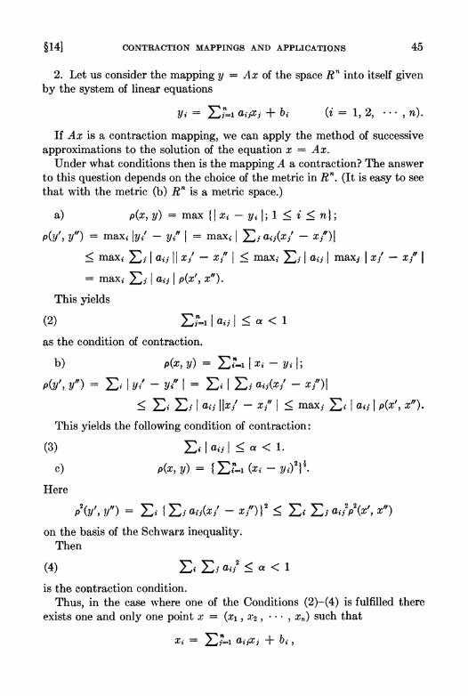
§14] CONTRACTION MAPPINGS AND APPLICATIONS 45
2. Let us consider the mapping y = Ax of the space R n into itself given by the system of linear equations
(i = 1, 2, "', n).
If Ax is a contraction mapping, we can apply the method of successive approximations to the solution of the equation x = Ax.
Under what conditions then is the mapping A a contraction? The answer to this question depends on the choice of the metric in Rn. (It is easy to see that with the metric (b) R n is a metric space.)
a) p(x,y) = max {I Xi - Yilil ~ i ~ n}i
p(y', y") = maXi Iy/ - y/' I = maXi I Lj aij(x/ - x/")I
~ maXi Lj I aii II x/ - x/, I ~ maXi Li I aij I maxi I x/ - x/ I = maxi Lj I aii I p(x', x").
This yields
(2) L/-I I aii I ~ a < 1
as the condition of contraction.
b) p(x, y) = Lf-l I Xi - Yi Ii p(y', y") = Li I y/ - y/' I = Li I Li aij(x/ - x;") I
~ Li Li I aii Ilx/ - x/' I ~ maxi Li I aij I p(x', x").
This yields the following condition of contraction:
(3)
c)
Here
Li I aii I ~ a < 1.
p(x,1/) = {Li'-l (Xi - Yi)2}i.
/(y', Y") = Li {Li aii(x/ - xl')}2 ~ Li Li ai//(x', x")
on the basis of the Schwarz inequality. Then
(4)
is the contraction condition. Thus, in the case where one of the Conditions (2)-(4) is fulfilled there
exists one and only one point x = (Xl, X2, ••• , xn ) such that

46 METRIC SPACES [CH. II
where the successive approximations to this solution have the form:
x (0) (XIO, X20, ... , X"O);
X(l) (X/, l"2\ ... , X"l);
where
X,·k = ~" a x k-l + b ~i=l if; i·
(Consequently anyone of the Conditions (2)-(4) implies that
¢ 0.)
ann - 11
Each of the Conditions (2)-(4) is sUfficient in order that the mapping y = Ax be a contraction. As concerns Condition (2) it. could have been proved that it is also necessary in order that the mapping y = Ax be a contraction (in the sense of the metric a)).
None of the Conditions (2)-(4) is necessary for the application of the method of successive approximations. Examples can be constructed in which anyone of these conditions is fulfilled but the other two are not.
If I ail I < lin (in this case all three conditions are fulfilled), then the method of successive approximations is applicable.
If I ail I = lin (in this case all three sums equal 1), it is easy to see that the method of successive approximations is not applicable.
§ 15. Applications of the principle of contraction mappings in analysis
In the preceding section there were given some of the simplest examples of the application of the principle of contraction mappings in one- and n-dimensional spaces. However, the most essential applications for analysis of the principle of contraction mappings are in infinite-dimensional function spaces. Further on we shall show how with the aid of this principle we can obtain theorems on the exist.ence and uniqueness of solutions for some types of differential and integral equations.
I. Let
(1) dyldx = f(x, y)
be a given differential equation with the initial condition
(2) y(XO) = Yo,

§15] C'ON'l'RA(,TIO~ MAPPINGS Ii\" ANALYSIS -47
where J(x, y) is defined and continuous in some plane region G which contains the point (xo , Yo) and satisfies a Lipschitz condition with respect to lJ:
i J(x, YI) - J(x, Y2)1 ~ M ! lh - Y21·
We shall prove that then 011 some closed interval Ix - Xo I < d there exists a unique solution y = cp(x) of the equation (1) satisfying the initial condition (2) (Picard's theorem).
Equation (1) together with the initial condition (2) is equivalent to the integral equation
(3) cp(x) = yo + JX J(t, cp(t» dt. "0
Since the function J(x, y) is continuous, we have I J(x, y) I < k in some region G' C G which contains the point (xo, Yo). Now we select ad> 0 such that the following conditions are fulfilled:
1) (x, y) E G' if I x - Xo I ~ d, I Y - lJo I ~ ltd;
2) Md < 1.
Denote by C* the space of continuous functions cp* which are defined on the closed interval I x - Xo I ~ d and are such that I cp* (.T) - lJo I ~ kd with the metric P(CPI ,CP2) = max" I CPI (x) - CP2(X) I·
It is easy to see that C* is a complete space. (This follows, for instance, from the fact that a closed subset of a complete space is a complete space.) Let us consider the mapping 1/; = Acp defined by the formula
1/;(x) = Yo + j'x J(t, cp(t» dt, Xo
where I x - Xo I ~ d. This is a contraction mapping of the complete space C* into itself. In fact, let cp E C*, I x - .To I ~ d. Then
11/;(x) - Yo I = I L J(t"cp(t» dti ~ kd
and consequently A(C*) C C*. Moreover, we have
I 1/;1 (x) - 1/;2(X) I ~ L IJ(t, CPI(t» - J(t, CP2(t» I dt
::; Md max" I CPI(X) - CP2(X) I.
Since Md < 1, the mapping A is a contraction. From this it follows that the operator equation cP = Acp (and consequently
equation (3) also) has one and only one solution. II. Let

48 METRIC SPACER [CH. II
(4) 'P/(x) = j;(XO ,'PI (X), ... , 'Pn(X)); i = 1,2, ... , Il;
be a given system of differential equations wit.h initial conditions
(5) i = 1, 2, ... , 11;
where the functions fiCa:, 11I, ... , Yn) are defined and continuous in some region G of the space R"+1 such that G contains the point (xo , 1/01 , ••• ,Yo,,) and satisfy a Lipschitz condition
I J ( (1) (1) f (2) (2) I i X, Yl ,"', Yn - . ; X, Yl ,"', Yn )
~ M maxi I Yi(l) - y/2) I; 1 ~ i ~ n\. We shall prove that then on some closed interval I x - Xo I < d there
exists one and only one system of solutions y,. = 'P,.(a:) satisfying system (4) and the initial conditions (5).
System (4) together with the initial conditions (5) is equivalent to the system of integral equations
(6) 'Pi(X) = YOi + JX Ji(t, 'PICt), "', 'Pn(t» dt; i = 1, ... , n. -"0
Since the function Ji is continuous in some region G' ~ G containing the point (xo, YOl, ... , 1/on), the inequalities I Ji(X, 111, ... , Yn)1 ~ K, where K is a constant, are fulfilled.
We now choose d > 0 to satisfy the following conditions:
1) (x, Yl, ... , Yn) E G if I x - Xo I ~ d, I !I; - Yo; I ~ Kd,
2) Md < 1.
We now consider the space Cn* whose elements are ordered systems ip = ('PI (X) , ... , 'Pn(X» consisting of n functions which are defined and continuous for all x for which 1:1: - ;)'0 I ~ d and such that I 'Pi(X) - YOi I ~ Kd, with the metric'
p(ip, ij,) = maxx , i I 'P;(x) - 1/;i(X) I· The mapping ij, = Aip, given by the system of integral equations
1/;i(X) = Yo; + r J(t, 'Pl(t), ... , 'Pn(t)) dt, xo
is a contraction mapping of the eomplet.e space C,,* into itself. In fact,
1/;i(1) (x) - 1/;/2) (x) = r' [J(t, 'PI (1), ••• , 'Pn (1) - J(t, 'PI (2), ••• , 'Pn (2» 1 dt "0
and consequently
max"" i 11/;/I)(X) - 1/;/2) (X) I ~ Md max", i I 'P/ 1) (X) - 'P/2)(x)l.
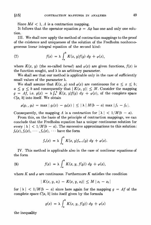
§15] CONTRACTION MAPPINGS IN ANALYSIS 49
Since M d < 1, A is a contraction mapping. It follows that the operator equation ip = Aip has one and only one solu
tion. III. We shall now apply the method of contraction mappings to the proof
of the existence and uniqueness of the solution of the Fredholm nonhomogeneous linear integral equation of the second kind:
(7) f(x) = }.. { K(x, y)f(y) dy + \O(x),
where K(x, y) (the so-called kernel) and \O(x) are given functions, f(x) is the function sought, and}.. is an arbitrary parameter.
We shall see that our method is applicable only in the case of sufficiently small values of the parameter}...
We shall assume that K(x"y) and \O(x) are continuous for a ~ x ~ b; a ~ y ~ b and consequently that j K(x, y)j ~ M. Consider the mapping g = Af, i.e. g(x) = }.. Jab K(x, y)f(y) dy + \O(x) , of the complete space C[a, b] into itself. We obtain
p(gl' g2) = max j gl(X) - g2(X) j ~ j }.. j1lf(b - a) max 1 f1 - f2 I. Consequently, the mapping A is a contraction for I}.. 1 < l/M(b - a).
From this, on the basis of the principle of cont.raction mappings, we can conclude that the Fredholm equation has a unique continuous solution for every I}..j < l/M(b - a). The successive approximations to this solut.ion: fO(X),!l(X), ... ,fn(x), ... have the form
fn(x) = }.. { K(x, y)fn-1(Y) dy + \O(x).
IV. This method is applicable also in the case of nonlinear equations of the form
(8) f(x) = }.. { K(x, y, f(y» dy + \O(x),
where K and \0 are continuous. Furthermore K satisfies the condition
I K(x, y, Zl) - K(x, y, Z2)j ~ M I Zl - Z2[
for I}.. I < l/M(b - a) since here again for the mapping g complete space C[a, b] into itself given by the formula
g(x) = }.. { K(x, y, f(y» dy + \OCI:)
the inequality
Af of the
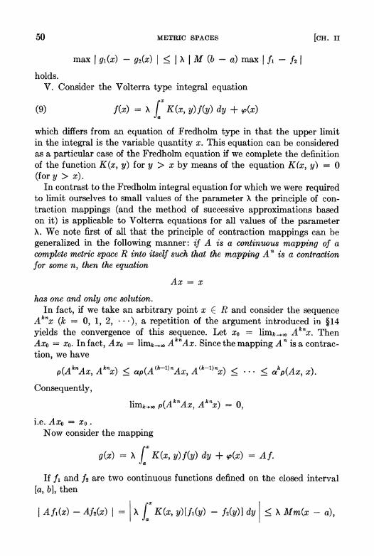
50 METRIC SPACES [CR. II
holds. V. Consider the Volterra type integral equation
(9) f(x) = A f K(x, y)f(y) dy + <p(x)
which differs from an equation of Fredholm type in that the upper limit in the integral is the variable quantity x. This equation can be considered as a particular case of the Fredholm equation if we complete the definition of the function K(x, y) for y > x by means of the equation K(x, y) = 0 (for y > x).
In contrast to the Fredholm integral equation for which we were required to limit ourselves to small values of the parameter A the principle of contraction mappings (and the method of successive approximations based on it) is applicable to Volterra equations for all values of the parameter A. We note first of all that the principle of contraction mappings can be generalized in the following manner: if A is a continuous mapping of a complete metric space R into itself such that the mapping A n is a contraction for some n, then the equation
Ax = x
has one and only one solution. In fact, if we take an arbitrary point x E R and consider the sequence
A knx (k = 0, 1, 2, ... ), a repetition of the argument introduced in § 14 yields the convergence of this sequence. Let Xo = limk .... '" A knx. Then Axo = Xo. In fact, Axo = limk .... '" A kn Ax. Since the mapping A n is a contraction, we have
peA knAx, A knx) :::; ap(A (k-l)n Ax, A (k-l)nx) :::; ... :::; akp(Ax, x).
Consequently,
i.e. Axo = Xo •
N ow consider the mapping
g(x) = A f K(x, y)f(y) dy + <p(x) = Af.
If /I and /2 are two continuous functions defined on the closed interval [a, b], then
I Afl(x) - Af2(x) I = I A f K(x, y)[/ICy) - My)] dy I :::; A Mm(x - a),
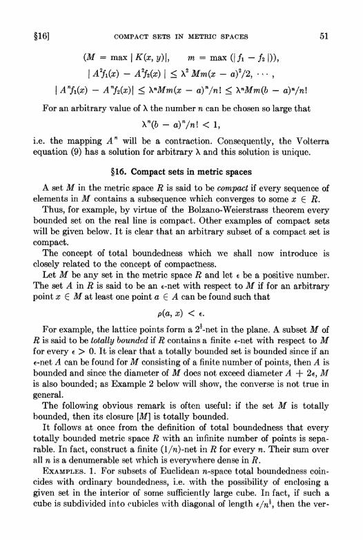
§16] COMPACT SETS IN METRIC SPACES 51
(M = max I K(x, y)l,
I A 2ft (X) - A2h(X) I ~ }..2 Mm(x - a)2/2, ... ,
I A njl(X) - A nh(x) I ~ }..nMm(x - a)n/n! ~ }..nMm(b - a)n/n!
For an arbitrary value of }.. the number n can be chosen so large that
i.e. the mapping A n will be a contraction. Consequently, the Volterra equation (9) has a solution for arbitrary}.. and this solution is unique.
§16. Compact sets in metric spaces
A set M in the metric space R is said to be compact if every sequence of elements in M contains a subsequence which converges to some x E R.
Thus, for example, by virtue of the Bolzano-Weierstrass theorem every bounded set on the real line is compact. Other examples of compact sets will be given below. It is clear t.hat an arbitrary subset of a compact set is compact.
The concept of total boundedness which we shall now introduce is closely related to the concept of compactness.
Let M be any set in the metric space R and let € be a positive number. The set A in R is said to be an €-net with respect to M if for an arbitrary point x E M at least one point a E A can be found such that
p(a, x) < €.
For example, the lattice points form a 2!-net in the plane. A subset M of R is said to be totally bounded if R contains a finite €-net with respect to M for every € > O. It is clear that a totally bounded set is bounded since if an €-net A can be found for M consisting of a finite number of points, then A is bounded and since the diameter of M does not exceed diameter A + 2€, JJ1 is also bounded; as Example 2 below will show, the converse is not true in general.
The following obvious remark is often useful: if the set M is totally bounded, then its closure [M] is totally bounded.
It follows at once from the definition of total bounded ness that every totally bounded metric space R with an infinite number of points is separable. In fact, construct a finite {I/n)-net in R for every n. Their sum over all n is a denumerable set which is everywhere dense in R.
EXAMPLES. 1. For subsets of Euclidean n-space total boundedness coincides with ordinary boundedness, i.e. with the possibility of enclosing a given set in the interior of some sufficiently large cube. In fact, if such a cube is subdivided into cubicles ,,·ith diagonal of length €/n!, then the ver-

52 Ml';TRIC SPACEK [CB. II
t.ices of these cubicles will form a finite E-net in the initial cube and therefore also in an arbitrary set which lies in the interior of this cube.
2. The unit sphere S in the space l2 is an example of a bounded Ret. which is not t.otally bounded. In fact, consider in S points of t.he form
CI = (1, 0, 0, ... ),
('2 = (0,1,0, ... ),
The distan('c hctween any two such points en and em (m ;6 11,) is 21. From this it is clear that in S there can be no finite E-net for any E :::; T~.
:t Consider in l2 the set IT of points x (XI, X2, ••• , X n , ••• ) which satisfy the following ronditions:
This set iR called the fundamental parallelopiped in the space l2 . It is an example of an infinit.e-dimensional totally bounded set. To prove that this set is totally bounded we proeeed as follows.
Let E > ° be given. Choose 11, so that (!)n < ej2. ASRodate with each point
(1)
in II the point.
(2) a:* = (a'l, .1:2, .. , ,a'n , 0, 0, ... )
from t.he same set.. Theil we havp
p(a:, x*) = (:Lk"=,,+1 :r/)] :::; (:Lk"..n+1 1/4k)1 < (!)" < E/2.
Thc :mhset 11* of points of the form (2) of II is t.otally bounded (since it is a hounded set. in n-dimensional Rpaee). We choose a finit.e (E/2)-net. in II*. It iH clear that it will he at the same timc an E-net for II.
The following theorem establiRhes the interrelation among the conecpt,s of eompaet.JWRS, eompletenesH, and t.otal houndedness.
THI~oJn;M 1. A necessary and 81lfficient condition that a subset J.lf of a com.plete m.etric space R be compact is that !If be totally bounded.
Proof. NecC8sit!/. We shall assume that !If is not totally bounded, i.e, we shall assume that. for some E > ° a finite E-net cannot be found in 111. We take an arbitrary point a'l in 1Il. Hinee, by assumption, t.here is no finit(, E-Ilet in lIf, a point .r2 E :AI can be found such that P(J'1 ,a'2) ~ E. Further, t.here exists a point a';\ E !If such t.hat p(.rl ,3'3) ~ E and p(:1'2 ,a':I) ~ E (otherwise the poillt.H .1'1 and :1'2 would fOI'l11 an E-nct in M), and so 011; ('ontinuing this process \\'(' COIIHtl'lwt a sequcnee Xl , :1'2, •.• , .1'" , ... of points in R which Hatisfy the ('ondition p(.l·m , :r1l ) ~ E for 1n ;6 1/.. It is dear that it is imposHibIe to select any eonvergent. subsequence from such a H<'querH'c.

§17] ARZELA'S THEOREM AND APPLICATIO:-;S 53
Sufficiency. Let R be complete and let M be totally boullded. We shall prove that in M "'e can select a convergent subsequenc(' from every sequence. Let {Xn} be a sequence of points in M. Ret
EI = 1, E~ = }, "', Ek = 1/ I .. , ...
and construct for every Ek a l'ol'l'cspondillg tillite Ek-lI('t ill J/: (k) (k) (k)
al ,a2, a"k
Describe about each of the points which forl11 a I-net in M a sphere of radius]. Since these spheres cover all of M and are finite in number, at leaRt one of them, let us call it SI , contains an infinite suhsequence XI (I),
:.1'2(1), ••• ,Xn(l>, ••• of the sequence {:.I',,}. Further, about each of the points which form a i-net in R we describe a sphere of radius i. Rince the number of these sphet'es is again finite, at least one of them, let us call it S2 , contains an infinite subsequence .1'1(2), X2(2) , ••• , .r,,(~\ ... of the sequence {Xn (I)}. Further, we find a sphere S3 of radius t containing an infinite
b (3) (3) (3) f' h I (2) } d f' h su sequence XI ,X2 ,"', .rn ,'" 0 t e sequenC'c .1'" ,an f;0 ort . N ow we choose from the sequences
XI (I), X2 (I)
Xl (2), X2 (2) ,
the "diagonal" subsequence
X (I) on ,
(I) (2) (11) ;l:l ,;~:2 ,"', .r" ,...;
thi:; subsequence is fundamental because all its terms beginning with .rn (n) lie in the interior of the sphere Sn of radius lin. Since the space R is complete, this suhsequence has a limit. This completeR the proof of the theorem.
The following generalization of Theorem] is often useful. THEOREM 2. A necessary and slI.fficient condition that a subset JJ of a
complete metric space R be compact is that for ('!Iery E ;::: 0 there exist in R a compact E-net for ."41.
Proof. The necessity is trivial; ,,-e shall prove the sufficiency. Let E > 0 be given and let A be a compact (E/2)-net for M. We choose a finite (E/2)net in A. It is clear that it will he a tinite E-net fol' .11; eonsequently, by virtue of the preC'eding theorem, til(' Ret .1[ if; ('ompaet.
§17. ArzeIa's theorem and its applications
The application of Theorems I and 2 of the pt'eceding section, which yield necessary and sufficient conditions for compactness to individual sperial cases, is 110t always simple. For sets, situated in Rome given special
54 METRIC SPACES [CR. II
space, special criteria for compactness can be given which are more suitable for practical application.
In analysis one of the more important metric spaces is the space era, b]. For subsets of this space the most important and frequently employed
criterion of compactness is given by Arzela's theorem. In order to formulate this theorem it is necessary to first introduce the
following concepts. A family I SO (x) } of functions defined on a closed interval is said to be
uniformly bounded if there exists a number M such that I so(x) I < M for all x and for all so belonging to the given family.
A family of functions is said to be equicontinuous if for every e > 0 there is a 5 > 0 such that
I SO(Xl) - SO (X2) I < e
for all Xl , X2 such that I Xl - X2 I < 5 and for all SO in the given family. ARZELA'S THEOREM. A necessary and sufficient condition that a family of
continuous functions defined on the closed interval [a, b] be compact in era, b] is that this family be uniformly bounded and equicontinuous.
Proof. Necessity. Let the set <I> be compact in era, b]. Then, by Theorem 1, §16, for each positive e there exists a finite (e/3)-net SOl , S02, ... , SOk in <1>. Each of the functions SOi , being a continuous function on a closed interval is bounded: I SOi I ~ Mi.
Set M = max Mi + e/3. By the definition of an (e/3)-net, for every so E <I> we have for at least one so; ,
p(SO, SOi) = max I so(x) - SOi(X) I < e/3.
Consequently
I SO I < I SOi I + e/3 < M; + e/3 < M.
Thus, <I> is uniformly bounded. Further, since each of the functions SOi is continuous and consequently
uniformly continuous on [a, b], for a given e/3 there exists a 5i such that
I SOi(XI) - SOi(X2) I < e/3
if I Xl - X2 I < 5i .
Set 5 = min 5i . Then for I Xl - X2 I < 5 and for any so E <1>, taking so; so that p(so, SOi) < e/3, we have:
I SO(XI) - SO(X2) I = I SO(Xl) - SOi(Xl) + SOi(Xl) - SOi(X2) + SO;(X2) - SO(X2) I ~ I SO(Xl) - SO,.(XI) I + I SOi(Xl) - SOi(X2) I + I SOi(X2) - SO(X2) I < e/3 + e/3 + e/3 = e.
The equicontinuity of <I> is thus proved.

§17] ARZELA'S THEOREM AND APPLICATIONS 55
SUfficiency. Let <P be a uniformly bounded and equicontinuous family of functions. In accordance with Theorem 1, §16, in order to prove its compactness in C[a, b] it is sufficient to show that for arbitrary e > 0 there exists for it in C[a, b] a finite e-net. Let
! cP ! ::; M for all cp E <P
and let 0 > 0 be chosen so that
! cp(Xl) - cp(X2) ! < e/5 for ! Xl - X2! < 0; Xl, X2 E [a, b];
and for all cp E <P. Subdivide the segment [a, b] on the x-axis by means of the points Xo = a, Xl , X2, .•• , Xn = b into intervals of length less than 0 and construct vertical lines at these points of subdivision. We subdivide the segment [-M, M] on the y-axis by means of the points Yo = - M, Yl , Y2, ... , Ym = M into intervals of length e/5 and construct horizontal lines at these points of subdivision. Thus we subdivide the rectangle a ::; X ::; b, - M ::; Y ::; M into cells with horizontal sides of length less than 0 and vertical sides of length e/5. We now assign to every function cp E <P a polygonal arc 1/;(x) with vertices at the points (Xk, Yl), i.e. at vertices of the constructed net and deviating at the points Xk from the function cp by less than e/5 (the existence of such a polygonal arc is obvious).
Since, by construction,
and
we have
! cp(Xk) - 1/;(Xk) ! < e/5,
I cp(Xk+l) - tf;(Xk+l) ! < e/5,
Since the function tf;(x) is linear between the points Xk and Xk+l , we have
! tf;(Xk) - tf;(x) I < 3e/5 for all x, Xk ::; X ::; Xk+l .
Now let x be an arbitrary point of the closed interval [a, b] and let Xk be the subdivision point chosen which is closest to x from the left. Then
I cp(x) - tf;(x) I ::; I cp(x) - cp(Xk) I + I cp(Xk) - tf;(Xk) I + I tf;(Xk) - tf;(x) I < e.
Consequently the polygonal arcs tf;(x) form an e-net with respect to <P. Their number is finite (since only a finite number of polygonal arcs can be drawn through a finite number of points); thus, <P is totally bounded. This proves the theorem completely.
ArzeUt's theorem has many applications. We shall demonstrate its

56 METRIC SPACES [CR. U
application in the example of the following existence theorem for ordinary differential equations with continuous right member.
THEOREM 2 (PEANO). Let
dy/dx = f(x, y)
be a given differential equation. If the function f(x, y) is continuous in a closed region G, then at least one integral curve of the given equation passes through each interior point (xo , Yo) of this region.
Proof. Since f(x, y) is continuous in the closed region, it is bounded:
If(x, y) 1 < M.
We draw straight lines with slopes M and - M through the point (xo , Yo). Further, we draw vertical lines x = a and x = b so that the two triangles cut off by them with the common vertex (Xo , Yo) lie entirely in the interior of the region G.
We now construct a so-called Euler polygonal arc for the given equation in the following way: we draw from the point (Xo, Yo) a straight line with the slope f(xo , yo). On this straight line we take a point (Xl, Yl) and draw through it a straight line with the slope f(Xl, Yl). On this straight line we take a point (X2 , Y2) and so forth. We now consider a sequence of Euler polygonal arcs Ll , L2 , '" , Lk , ••• , passing through the point (Xo , Yo) such that the length of the greatest of the links of the polygonal arc Lk tends to zero as k ~ 00. Let ~k(X) be the function whose graph is the polygonal arc L k • The functions ~ , ~, ... , ~k, ••• possess the following properties: they are 1) defined on the same segment [a, b], 2) all bounded, and 3) equicontinuous.
On the basis of Arzela.'s theorem, we can choose a uniformly convergent subsequence from the sequence {~k(X)}. Let this sequence be
~(l)(x), ~(2)(X), '" , ~(k)(X), ••••
We set ~(x) = lim,... .. ~(k)(X). It is clear that ~(Xo) = Yo. It remains to verify that ~(x) satisfies the given differential equation on the closed interval [a, b]. To do this it is necessary to show that for arbitrary E > 0
I ~(x:l := :~x') - f(x', ~(x')) I < E
provided the quantity 1 x" - x' 1 is sufficiently small. To prove this it is sufficient in turn to establish that for sufficiently large k
~ x" -~, x _ f(x',~(x')) < E I (k)(") (k)( ') I X - X
if only the difference 1 x" - x' 1 is sufficiently small.

§18j COMPACTA 57
Since f(x, y) is continuous in the region G, for arbitrary E > 0 an ." > 0 can be found such that
f(x' , y') - E < f(x, y) < f(x /, y') + E, (y' = rp(X')),
if
I x - x' I < 2." and I y - y' I < 4M.".
The set of points (x, y) E G which satisfy both these inequalities form some rectangle Q. Now let K be so large that for all k > K
I rp(x) - rp(k)(X) I < M."
and all links of the polygonal arc Lk have length less than .". Then if I x' - x I < 2.", all the Euler polygons y = rp(k)(X) for which k > K lie entirely in the interior of Q.
Further, let (ao, bo), (al, bl), .. , , (an+l, bn+l) be vertices of the polygonal arc y = rp(k)(X), where
ao ~ x' < al < <Z2 < ... < an < x" ~ an+l
(we assume x" > x' for definiteness; we can consider the case x" < x' analogously). Then
rp(k)(al) - rp(k)(X' ) = f(ao, bO)(al - x');
rp(k)(ai+l) - rp(k)(ai) = f(ai, bi)(ai+l - a.),
rp(k)(X") - rp(k)(a..) = f(an , bn)(x" - an).
From this it follows that for I x" - x' I < .",
i = 1,2, ... , n - 1;
[f(X', y') - E](al - x') < rp(k)(al) - rp(k)(X' ) < [f(x/, y') + E](al - x');
U(x' , y') - E](ai+l - ai) < rp(k)(ai+l) - rp(k)(ai)
< [f(X', y') + E](ai+l - a.), i = 1,2, .. , ,n - 1;
[f(x' , y') - E](X" - an) < rp(k)(X") - rp(k)(an ) < rJ(x' , y') + E](X" - an).
Summing these inequalities, we obtain
[f(X', y') - E](X" - x') < rp(k)(X") - rp(k)(X' ) < rJ(x' , y') + E](X" - x'),
which was to be proved. The solution rp(x) thus obtained will in general not be the unique solution
of the equation y' = f(x, y) which passes through the point (xo, yo).
§18. Compacta
In §16 we said that a subset M of a metric space R is compact if every sequence of elements in M has a subsequence which converges to some x E R.

58 METRIC SPACES [CR. II
In this connection the limit point x might belong but it also might not belong to the set M. If from every sequence of elements in M it is possible to select a subsequence which converges to some x belonging to M, then the set M is said to be compact in itself. For the space R itself (as moreover also for all its closed subsets) the concepts of compactness and compactness in itself coincide. A compact metric space is called a compactum for brevity.
Inasmuch as compactness in itself of a set is an intrinsic property of this set which does not depend on the metric space in which it is embedded, it is natural to limit oneself to the study of compacta, i.e. to consider each such set simply as a separate metric space.
THEOREM 1. A necessary and sufficient condition that a set M compact in a metric space R be a compactum is that M be closed in R.
Proof. Necessity. Suppose M is not closed; then we can find in M a sequencc Ix .. } which converges to a point x EE M. But then this sequence cannot contain a subsequence which converges to some point y E M, i.e. M cannot be a compactum.
Sufficiency. Since M is compact, every sequence Ix .. } c M contains a subsequence which converges to some x E R. If M is closed, x E M, i.e. M is compact in itself.
The next corollary follows from this and Theorem 1, §16. COROLLARY. Every closed bounded subset of Euclidean space is a compactum. TRIWREM 2. A necessary and sufficient condition that a metric space be a
compactum is that it be: 1) complete and 2) totally bounded. The proof of this theorem is made by a verbatim repetition of the proof
of Theorem 1, §16. THEOREM 3. Every compactum K contains a countable everywhere dense set. Proof. Since a compactum is a totally bounded space, K contains a finite
(l/n)-net: aI, <Z2, ••• , am .. for every n. The union of all these E-nets is a finite or denumerable set. This and Theorem 4, §1O, imply the following corollary.
COROLLARY. Every compactum has a countable basis. THEOREM 4. A neCeSSaT1j and sufficient condition that the metric space R be
a compactum is that either of the following two conditions holds: 1) A n arbitrary open covering IDa} of the space R contains a finite sub
covering; 2) An arbitrary system IF a} of closed sets in R with the finite intersection
property has a nonvoid intersection. (A system of sets is said to have the finite intersection property if an arbitrary finite number of these sets has nonvoid intersection.)
Proof. We note first of all that the equivalence of the two conditions formulated abov~ follows directly from the principle of duality (§1). In fact, if IDa} is an open covering of the space R, then IR '" Oa} is a system

§18] COMPACTA 59
of closed sets satisfying the condition
n(R '" 0 .. ) = o. The condition that we can select a finite subcovering from {O .. } is equiva
lent to the fact that the system of closed sets {R '" O .. } cannot have the finite intersection property if it has a void intersection.
We shall now prove that Condition 1 is necessary and sufficient that R be a compactum.
Necessity. Let R be a compactum and let {O .. } be an open covering of R. We choose in R for each n = 1, 2, ... a finite (l/n)-net consisting of the points ak (n) and we enclose each of these points with the sphere
S(ak(n), lin)
of radius lin. It is clear that for arbitrary n
R = UkS(A k (n), lin).
We shall assume that it is impossible to choose a finite system of sets covering K from {O .. }. Then for each n we can find at least one sphere S(ak(n)(n), lin) which cannot be covered by a finite number of the sets 0 ... We choose such a sphere for each n and consider the sequence of their centers {ak(n) (n)}. Since R is a compactum, there exists a point ~ E R which is the limit of a subsequence of this sequence. Let Ofj be a set of {O .. } which contains~. Since Ofj is open, we can find an E > 0 such that S{~, E} C Ofj . We now choose an index n and a point ak(n) (n) so that p(~, ak(n) (n») < E/2, lin < E/2. Then, obviously, S(ak(n)(n), lin) c Ofj, i.e. thesphereS(ak(n)(n), lin) is covered by a single set Ofj . The contradiction thus obtained proves our assertion.
Sufficiency. We assume that the space R is such that from each of its open coverings it is possible to select a finite subcovering. We shall prove that R is a compactum. To do this it is sufficient to prove that R is complete and totally bounded. Let E > O. Take a neighborhood O(x, E) about each of the points x E R; we then obtain an open covering of R. We choose from this covering a finite subcovering O(Xl , E), ... ,O(xn , E). It is clear that the centers Xl, ••• , Xn of these neighborhoods form a finite E-net in R. Since E > 0 is arbitrary, it follows that R is totally bounded. Now let {Sn} be a sequence of nested closed spheres whose radii tend to zero. If their intersection is void, then the sets R '" S" form an open covering of R from which it is impossible to select a finite subcovering. Thus, from Condition 1 it follows that R is complete and totally bounded, i.e. that R is compact.
THEOREM 5. The continuous imO{Je of a compactum is a compactum. Proof. Let Y be a compactum and let Y = cp(X) be its continuous image.
Further, let {O .. } be an open covering of the space Y. Set U .. = cp-l(O .. ).

60 METRIC SPACES [CH. II
Since the inverse image of an open set under a continuous mapping is open, it follows that {U a} is an open covering of the space X. Since X is a compactum, we can select a finite subcovering U1 , U2, ... , Un from the covering {Ua }. Then the corresponding sets 0 1 , O2 , ••• , 0" form a finite subcovering of the covering {O a}.
THBOREM 6. A one-to-one mapping of a compactum which is continuous in one direction is a homeomorphism.
Proof. Let cp be a one-to-one continuous mapping of the compactum X onto the compactum Y. Since, according to the preceding theorem, the continuous image of a compactum is a compactum, the set cp(M) is a compactum for an arbitrary closed M C X and consequently cp(M) is closed in Y. It follows that the inverse image under the mapping cp -1 of an arbitrary closed set M C X is closed; i.e. the mapping cp -1 is continuous.
RI<;MARK. The following result follows from Theorem 6: if the equation
(3) dy/dx = f(x, y),
where the function f(x, y) is continuous in a closed bounded region G which contains the point (xo, Yo) for every Yo belonging to some closed interval [a, b], has a unique solution satisfying the initial condition y(xo) = Yo , then this solution is a continuous function of the initial value Yo .
In fact, since the function f(x, y) is continuous in a closed bounded region, it is bounded and consequently the set P of solutions of equation (3) corresponding to initial values belonging to the closed interval [a, b] is uniformly bounded and equicontinuous. Moreover, the set P is closed. In fact, if {cp,,(x)} is a sequence of solutions of equation (3) which converges uniformly to a function cp(x), then cp(x) is also a solution of equation (3) since, if
cp,,' = f(x, CPn(x)),
then passing to the limit as n ~ 00, we obtain
cp' = f(x, cp(x)).
We have
cp(xo) = lim cp,,(xo) E [a, b].
In virtue of Arzela's theorem and Theorem 1 of this section it follows from this that P is a compactum.
We set the point cp(xo) of the closed interval [a, b] into correspondence with each solution cp(x) of equation (3). By assumption this correspondence is one-to-one. Moreover, since

§18] COMPACTA 61
the mapping \O(x) -4 \O(xo) is continuous. By virtue of Theorem 6 the inverse mapping is also continuous and this then signifies the continuous dependence of t.he solutions on the initial conditions.
K ow let C xy be the set of all continuous mappings y = f(x) of a compactum X into a compactum Y. We introduce distance into CXy by means of the formula
p(f, g) = sup {p[J(x), g(x)]; x EX}.
It is easy to verify that in this way CXy is transformed into a metric space.
THEOREM 7 (GgNEUALIZI';n THEOREM OF ARZEU). A necessary and sufficient condition that a set DeC xy be compact in C XY is that in D the functions y = f(x) be equicontinuotls, i.e. that for arbitrary E > 0 there exist a Ii > 0 such that
(1) p(x', x") < Ii implies
(2) p[f(x'), f(x")] < E
for arbitrary f in D and x', x" in X. Proof. We embcd CXY in the space Mxy of all mappings of the compactum
X into the compactulU Y with the same metric
p(f, g) = sup {p[J(x), g(x)]; x E X}
which was introduc'ed in C xy and prove the compactness of the set D in M xy . Since Cxy is closed in M xy , the compactness of the set D in Mxy will imply its compaetness in CXY • (That CXY is closed in Mxy follows from the fact that the limit of a uniformly convergent sequence of continuous mappings is also a continuous mapping. The indicated assertion is a direct gencralization of the known theorem in analysis and is proved in exactly the same way.)
Let E > 0 be arbitrary and choose Ii such that (1) implies (2) for all f in D and all x', x" in X. Let the points Xl , X2, ••• ,Xn form a (1i/2)-net in X. It is easy to see that X can be represented as the sum of nonintersecting sets Ei such that x, y E Ei implies that p(x, y) < Ii. In fact, it is sufficient to set"for example,
We now consider in the compactum Y a finite E-net YI, Y2, ... , Ym ; we denote the totality of functions g(x) which assume the values Y j on the sets Ei by L. The number of such functions is clearly finite. We shall show that they form a 2E-net in Mxy with respect to D. In fact, let fED. For

62 METRIC SPACES [CH. II
every point Xi in Xl, ... ,Xn we can find a point.Yj in Yl, ... , Ym such that
p[f(Xi), Y j] < ~.
Let the function g(x) E L be chosen so that g(Xi) = Y j • Then
pff(.g;), g(x)] ::; p[f(x), f(Xi)] + P[f(Xi), g(Xi)] + p[g(x), g(Xi)] < 2~
if i is chosen so that X E ~i. From this it follows that pC!, g) < 2~ and thus the compactness of D in
Mxy and consequently in CXy also is proved.
§19. Real functions in metric spaces
A real function on a space R is a mapping of R into the space Rl (the real line).
Thus, for example, a mapping of Rn into Rl is an ordinary real-valued function of n variables.
In the case when the space R itself consists of functions, the functions of the elements of R are usually called functionals. We introduce several examples of functionals of functions f(x) defined on the closed interval [0, 1]:
FlC!) = sup f(x);
F 2(f) = inf f(x);
Fa(f) = f(xo) where Xo E [0, 1];
F4(f) = ~[f(xo), f(Xl), ... ,f(xn )] where Xi E [0, 1]
and the function ~(Yl' ... , Yn) is defined for all real Yi ;
Fo(f) = [ ~[x, f(x)] dx,
where ~(x, y) is defined and continuous for all ° ::; x ::; 1 and all real y;
F 6(f) = !'(xo);
F7(f) = [ [1 + !,2(X)]! dx;
Fs(f) = [ I !'(x) I dx.
Functionals can be defined on all of R or on a subset of R. For example, in the space C the functionals Fl , F2 , Fa, F4 , Fa are defined on the entire space, F6(f) is defined only for functions which are differentiable at the point Xo , F7(f) for functions for which [1 + r(x)]~ is integrable, and FsC!) for functions for which I f'(x) I is integrable.

§19] REAL FUNCTIONS IN METRIC SPACES 63
The definition of continuity for real functions and functionals remains the same as for mappings 111 general (see §12).
For example, FI(f) is a continuous functional in C since
p(f, g) = sup 1 f - gland 1 sup f - sup g 1 ~ sup 1 f - g I;
F2 , Fa, Fa are also continuous functionals in C; F4 is continuous in the space C if the function!p is continuous for all arguments; F6 is discontinuous at every point in the space C for which it is defined. In fact, let g(x) be such that g'(xo) = 1,1 g(x) 1 < E and f = fo + g. Then f'(xo) = fo'(xo) + 1 and p(f, fo) < E. This same functional is continuous in the space C(1) of functions having a continuous derivative with the metric
p(f, g) = sup [I f - g 1 + 1 f' - g'l1;
F7 is also a discontinuous functional in the space C. In fact, let fo(x) == 0 and fn(x) = (lin) sin 27Tnx. Then p(fn ,fo) = lin ~ o. However, F7(!n) is a constant (it does not depend on n) which is greater than (17)1 and F7(fo) = 1.
Consequently, F7(f) is discontinuous at the point fo . By virtue of this same example Fs(f) is also discontinuous in the space
C. Both functionals F7 and Fs are continuous in the space C(l). The following theorems which are the generalizations of well-known
theorems of elementary analysis are valid for real functions defined on compacta.
THEOREM 1. A continuous real function defined on a compactum is uniformly continuous.
Proof. Assume f is continuous but not uniformiy continuous, i.e. assume there exist Xn and xn' such that
1 Xn - xn ' 1 < lin and 1 f(xn) - f(xn') 1 ~ E.
From the sequence Ixn } we can choose a subsequence Ixnk } which con-verges to x. Then also I xnk'} ~ x and either 1 f(x) - f(xn') 1 ~ E/2 or 1 f(x) - f(xn ) 1 ~ E/2, which contradicts the continuity of f(x).
THEOREM 2. If the function f(x) is continuous on the compactum K, then f is bounded on K.
Proof. If f were not bounded on K, then there would exist a sequence I Xn} such that f(x n) ~ 00 • We choose from I xn} a subsequence which converges to x: Ixnk } ~ x. Then in an arbitrarily small neighborhood of x the function f(x) will assume arbitrarily large values which contradicts the continuity of f.
THEOREM 3. A function f which is continuous on a compactum K attains its least upper and greatest lower bounds on K.
Proof. Let A = sup f(x). Then there exists a sequence Ixn } such that
A > f(x n ) > A - lin.

G4 MEnne SPACES [CII. II
We choose a convergent subsequence from {xn } : {xnk } ~ x. By continuity, f(x) = A. The proof for inf f(x) is entirely analogous.
Theorems 2 and 3 allow generalizations to an even more extensive class of functions (the so-called semicontinuous functions).
A function f(x) is said to be lower (upper) semicontinnous at the point Xo if for arbitrary E > 0 there exists a a-neighborhood of :ro in which f(x) > f(xo) - E, (f(x) < f(xo) + E).
For example, the function "integral part of :1:", f(a:) = E(:r), is upper semicontinuous. If we increase (decrease) the yalue of f(.ro) of a cOllt.inuous function at a single point Xo , we obtain a fWlction which is upper (lower) semicontinuous. If f(x) is upper semicontinuous, then -f(x) is lower semicontinuous. These two remarks at once permit us to construct a large number of examples of semicontinuous functions.
We shall also consider functions which assume the "alues ± ex:. If f(Xo) == - ex: , then f(x) will be assumed to be lower semicontinuous at :l"o and upper semicontinuous at Xo if for arbitrary h > 0 there is a neighborhood of the point Xo in which f(x) < - h.
If f(xo) = + co, then f(x) "ill be assumed to be upper semicontinuous at Xo and lower semicontinuous at Xo if for arbitrary h > 0 there is a neighborhood of the point Xo in whichf(x) > h.
The upper limit J(xo) of the function f(x) at the point Xo is the lim .... o
{sup [f(x); x E S(xo, E)]}. The lower limit [(xo) is the lim .... o {inf [f(x); x E S(xo, E)]}. The difference wf(xo) = J(Xo) - [(xo) is the oscillation of the function f(x) at the point Xo . It is easy to see that a necessary and sufficient condition that the function f(x) be continuous at the point a·o is that wf(xo) = 0, i.e. that J(xo) = [(xo).
]'or arbitrary f (x) the function J(x) is upper semicontinuous and the function [(x) is lower semicontinuous. This follows easily from the definition of the upper and lower limits.
We now consider several important examples of semicontinuous functionals.
Let f(x) be a real function of a real variable. For arbitrary real a and b such that f(x) is defined on the closed interval [a, b] we define the t{)tal variation of the functionf(x) on [a, b] to be the functional
Vab(f) = sup Ei=l 1 f(xi) - f(xi-l) 1
where a = Xo < Xl < X2 < ... < x" == b and the least upper bound is taken over all possible subdivisions of the closed interval [a, b].
For a monotone function Vab(f) == 1 feb) - f(a) I. For a piecewise monotone function Vab(f) is the sum of the absolute values of the increments on the segments of monotonicity. For such functions

§19] REAL FUNCTIONS IN METRIC SPACES 65
is attained for some subdivision. We shall prove that the functional Vab(J) is lower semicontinuous in the
space M of all bounded functions of a real variable with metric p(j, g) = sup I f(x) - g(x) I (it is clear that C is a subspace of the space M), i.e. that for arbitrary f and E > 0 there exists a 0 such that Vab(g) > Vab(f) - E for p(f, g) < o.
We choose a subdivision of the closed interval [a, b] such that
Lf-l I f(Xi) - f(Xi-l) I > Vab(f) - E/2.
Let 0 = E/4n. Then if p(g, f) < 0, we have
Li-l I f(:ri) - f(Xi-l) I - Li-l I g(Xi) - g(Xi_l) I < E/2
and consequently
Vab(g) ~ Li-l I g(Xi) - g(Xi-l) I > Vab(f) - E.
In the case Vab(J) = 00 the theorem remains valid since then for arbitrary H there exists a subdivision of the closed interval [a, b] such that
Li-l I f(Xi) - f(Xi-l) > H
and 0 can be chosen such that
Li-l I f(Xi) - f(Xi-l) I - Li-l I g(Xi) - g(Xi-l) I < E.
Then Vab(g) > H - E, i.e. Vab(g) ~ H, so that Vab(g) = 00.
The functional Vab(J) is not continuous as is easily seen from the following example. Let f(x) == 0, gn(x) = (lin) sin nx. Then p(gn, f) = lin, but l'O"(gn) = 2 and Vo"(J) = o.
Functions for which Vab(j) < 00 are said to be functions of bounded (or finite) variation. The reader can find more information about the properties of such functions in the books by Aleksandrov and Kolmogorov: Introduction to the Theory of Functions of a Real Variable, Chapter 7, §7; N atanson: Theory of Functions of a Real Variable, Chapter 8; and Jeffery: The Theory of Functions of a Real Variable, Chapter 5.
We shall define the length of the curve y = f(x) (a ~ x ~ b) as the functional
Lab(J) = sup Li-l {(Xi - Xi-I)2 + [f(Xi) - f(Xi_I)]2j\
where the least upper bound is taken over all possible subdivisions of the closed interval [a, b]. This functional is defined on the entire space M. For continuous functions it coincides with the value of the limit
lim Li-l {(Xi - Xi_I)2 + [f(Xi) - f(Xi_I)]2jt as maXi I Xi - Xi-l I ~ O.

66 METRIC SPACES [CH. II
Finally, for functions with continuous derivative it can be written in the form
{ [1 + j'2(X)]i dx.
The functional Lab(f) is lower semicontinuous in M. This is proved exactly as in the case of the functional Vab(j).
Theorems 2 and 3 established above generalize to semicontinuous functions.
THEOREM 2a. A finite function which is lower (upper) semicontinuous on a compactum K is bounded below (above) on K.
In fact, let f be finite and lower semicontinuous and let inf f(x) = - oc •
Then there exists a sequence {xnl such that f(xn) < -no We choose a subsequence {xnkl ~ Xo . Then, by virtue of the lower semicontinuity of f, f(xo) = - co, which contradicts the assumption that f(x) is finite.
In the case of an upper semicontinuous function the theorem is proved analogously.
THEOREM 3a. A finite lower (upper) semicontinuous function defined on a compactum K attains its greatest lower (least upper) bound on K.
Assume the function f is lower semicontinuous. Then by Theorem 2 it has a finite greatest lower bound and there exists a sequence {xnl such that f(xn) ~ inf f(x) + lin. We choose a subsequence {xnkl ~ Xo . Then f(xo) = inf f(x) since the supposition that f(xo) > inf f(x) contradicts the lower semicontinuity of f.
The theorem is proved analogously for the case of an upper semicontinuous function.
Let K be a compact metric space and let CK be the space of continuous real functions defined on K with distance function p(f, g) = sup I f - g I. Then the following theorem is valid.
THEOREM 4. A necessary and sufficient condition that the set D C CK be compact is that the functions belonging to D be uniformly bounded and equicontinuous (Arzela,'s theorem for continuous functions defined on an arbitrary compactum).
The sufficiency follows from the general Theorem 7, §18. The necessity is proved exactly as in the proof of Arzela's theorem (see §17).
§20. Continuous curves in metric spaces
Let P = f(t) be a given continuous mapping of the closed interval a ~ t ~ b into a metric space R. When t runs through the segment from a to b, the corresponding image point P runs through some "continuous curve" in the space R. We propose to give rigorous definitions connected with the above ideas which were stated rather crudely just now. We shall

§20] CONTINUOUS CURVES IN METRIC SPACES 67
FIG. 11 FIG. 12 FIG. 13
y y
t t FIG. 14 FIG. 15
consider the order in which the point traverses the curve an essential property of the curve itself. The set shown in Fig. 11, traversed in the directions indicated in Figs. 12 and 13, will be considered as distinct curves. Ai!, another example let Us consider the real function defined on the closed interval [0, 1] which is shown in Fig. 14. It defines a "curve" situated on the segment [0, 1] of the y-axis, distinct from this segment, traversed once from the point 0 to the point 1, since the segment [A, B) is traversed three times (twice upward and once downward).
However, for the same order of traversing the points of the space we shall consider the choice of the "parameter" t unessential. For example, the functions given in Figs. 14 and 15 define the same "curve" over the y-axis although the values of the parameter t corresponding to an arbitrary point of the curve can be distinct in Figs. 14 and 15. For example, in Fig. 14 to the point A there correspond two isolated points on the t-axis, whereas in Fig. 15 to the point A there correspond on the t-axis one isolated point and the segment lying to the right (when t traverses this segment the point A on the curve remains fixed). [Allowing such intervals of constancy of the point P = f(t) is further convenient in the proof of the compactness of systems of curves.]
We pass over to formal definitions. Two continuous functions

68 METRIC SPACES [CR. II
defined, respectively, on the closed intervals
a' ~ t' ~ b' and a" ~ til ~ b"
are said to be equivalent if there exist two continuous nondecreasing functions
t' = ~1(t) and til = ~2(t)
defined on a closed interval a ~ t ~ b and possessing the properties
~1(a) = a', ~1(b) = b',
~2(a) = a", ~2(b) = b",
Il[~I(t)] = h[~2(t)]
for all t E [a, b]. It is easy to see that the equivalence property is reflexive (f is equivalent
to f), symmetric (if II is equivalent to h , then 12 is equivalent to II), and transitive (the equivalence of II and 12 together with the equivalence of 12 and Is implies the equivalence of II and is). Therefore all continuous functions of the type considered are partitioned into classes of equivalent functions. Every such class also defines a continuous curve in the space R.
It is easy to see that for an arbitrary function P = fI(t') defined on a closed interval [a', b'] we can find a function which is equivalent to it and which is defined on the closed interval [a", b"] = [0, 1]. To this end, it is sufficient to set
t' = ~1(t) = (b' - a')t + a', til = ~2(t) = t.
(We always assume that a < b. However we do not exclude "curves" consisting of a single solitary point which is obtained when the function f(t) is constant on [a, b]. This assumption is also convenient in the sequel.) Thus, we can assume that all curves are given parametrically by means of functions defined on the closed interval [0, 1].
Therefore it is expedient to consider the space GIll. of continuous mappings of the closed interval I = [0, 1] into the space R with the metric p(f, g) =
SUPt p[I(t), g(t)]. We shall assume that the sequence of curves L 1 , L 2 , ••• , L n , ••• con
verges to the curve L if the curves Ln can be represented parametrically in the form
P = I n(t), o ~ t ~ 1,
and the curve L in the form
P = I(t), o ~ t ~ 1,
so that p(f, In) -7 0 as n -7 00.

§20} CONTINUOUS CURVES IN METRIC SPACES 69
We obtain Theorem 1 if we apply the genera1ized ArzelA theorem (Theorem 7, §18) to the space ClIl.
THEOREM 1. If the 8equence of curve8 Ll , L2 , ••• , L,., ... lying in the compactum K can be repre8ented parametrically by mean8 of equicontinuou8 function8 defined on the cl08ed interval [0, 1], then this 8equence contain8 a convergent sub8equence.
We shall now define the length of a curve given parametrically by means of the function P = f(t), a ~ t ~ b, as the least upper bound of sums of the form
where the points ti are subject only to the following conditions:
a ~ to ~ tl :$ .•. :$ ti ~ ... :$ t,. = b.
It is easy to see that the length of a curve does not depend on the choice of its parametric representation. If we limit ourselves to parametric representations by functions defined on the closed interval [0, 1], then it is easy to prove by considerations similar to those of the preceding section that the length of a curve is a lower semicontinuous functional of f (in the space C IR). In geometric language this result can be expressed in the form of such a theorem on semicontinuity.
THEOREM 2. If the sequence of curve8 Ln converge8 to the curve L, then the length of L i8 not greater than the greate8t lower bound of the length8 of the curve8 L".
We shall now consider specially curve8 of finite length or rectifiable curve8. Let the curve be defined parametrically by means of the function P = f(t), a :$ t :$ b. The function f, considered only on the closed interval [a, T], where a :$ T ~ b, defines an "initial segment" of the curve from the point P a = f(a) to the point P T = f(T). Let 8 = q;(T) be its length. It is easily established that
P = g(8) = f[q;-1(8)]
is a new parametric representation of the same curve. In this connection 8
runs through the closed interval 0 :$ 8 :$ S, where S is the length of the entire curve under consideration. This representation satisfies the requirement
p[g(81), g(82)] :$ I 82 - 81 I (the length of the curve is not less than the length of the chord).
Going over to the closed interval [0, 1] we obtain the parametric representation
P = F(T) = g(8), T = 8/S

70 METRIC SPACES
which satisfies the following Lipschitz condition:
p[J?(n), F(T2)] ~ S I Tl - T2 \.
[CH. II
We thus see that for all curves of length S such that S ~ M, where M is a constant, a parametric representation on the closed interval [0, 1] by means of equicontinuous functions is possible. Consequently, Theorem 1 is applicable to such curves.
We shall show the power of the general results obtained above by applying them to the proof of the following important proposition.
THEOREM 3. If two points A and B in the compactum K can be connected by a continuous curve of finite length, then among all such curves there exists one of minimal length.
In fact, let Y be the greatest lower bound of the lengths of curves which connect A and B in the compactum K. Let t.he lengths of the curves L1 ,
L2 , ... , L", .•• connecting A with B tend to Y. From the sequence L" it is possible, by Theorem 1, to select a convergent subsequence. By Theorem 2 the limit curve of this subsequence cannot have length greater than Y.
We note that even when K is a closed smooth (i.e. differentiable a sufficient number of times) surface in three-dimensional Euclidean space, this theorem does not follow directly from the results established in usual differential geometry courses where we restrict ourselves ordinarily to the case of sufficiently proximate points A and B.
All the arguments above would take on great clarity if we formed of the set of all curves of a given metric space R a metric space. This can be done by introducing the distance between two curves Ll and L2 by means of the formula
p(Ll' L2) = inf p(fl ,h),
where the greatest lower bound is taken over all possible pairs of parametric representations
p = h(t) (0 ~ t ~ 1)
of the curves Ll and L2 , respectively. The proof of the fact that this distance satisfies the axioms of a metric
space is very straightforward with the exception of one point: there is some difficulty in proving that p(LI ,L2) = 0 implies that the curves Ll and L2 are identical. This fact is an immediate consequence of the fact that the greatest lower bound in the formula which we used in the definition of the distance p(LI , L2) is attained for a suitable choice of the parametric representations fl and 12 . But the proof of t.his last assertion is also not very straightforward.

Chapter III
NORMED LINEAR SPACES
§21. Definition and examples of normed linear spaces
DEFINITION 1. A set R of elements x, y, z, ... is said to be a linear space if the following conditions are satisfied:
I. For any two elements x, y E R there is uniquely defined a third ele-ment z = x + y, called their sum, such that
1) x + y = y + x, 2) x + (y + z) = (x + y) + z, 3) there exists an element 0 having the property that x + 0 = x for all
x E R, and 4) for every x E R there exists an element -x such that x + (-x) = O. II. For an arbitrary number a and element x E R there is defined an ele-
ment ax (the product of the element x and the number a) such that 1) a(8x) = (a8)x, and 2) l·x = x. III. The operations of addition and multiplication are related in the
following way: 1) (a + (3)x = aX + (3x, and 2) a(x + y) = ax + ay. Depending on the numbers admitted (all complex numbers or only the
reals), we distinguish between complex and real linear spaces. Unless otherwise stated we shall consider real linear spaces. In a linear space, besides the operations of addition and multiplication by scalars, usually there is introduced in one way or another the operation of passage to the limit. It is most convenient to do this by introducing a norm into the linear space.
A linear space R is said to be nonned if to each element x E R there is made to correspond a nonnegative number II x II which is ("aIled the norm of x and such that:
1) II x II = 0 if, and only if, x = 0, 2) II aX II = I a III x II, 3) II x + y II ~ II x II + II y I!·
lt is easy to see that every normed space is also a metric space j it is sufficient to set p(x, y) = II x - y II. The validity of the metric space axioms follows directly from Properties 1-3 of the nom1.
A complete normed space is said to be a Banach space, a space of Banach type, or, more briefly, a B-space.
EXAMPLES OF NORMED SPACES. 1. The real line with the usual arithmetic definitions is the simplest example of a normed space. In this case the norm is simply the absolute value of the real number.
71

72 NORMED LINEAR SPACES [CR. III
2. Euclidean n-space, i. e. the space consisting of all n-tuples of real numbers: x = (Xl, X2, ••• , Xn) in which the norm (i. e. the length) of the vector is defined to be the square root of its scalar square,
" x" = (L:f=l x/)\ is also a normed linear space.
In an n-dimensional linear space the norm of the vector X = (Xl, X2 ,
••• , Xn) can also be defined by means of the formula
(p ~ 1).
We also obtain a normed space if we set the norm of the vector X = (Xl, X2, • •• ,xn) equal to the max I IXk I; 1 ~ k ~ n}.
3. The space C[a, b] of continuous functions with the operations of addition and multiplication by a scalar which are usual for functions, in which
II f(t) " = max II f(t) I; a ~ t ~ b},
is a normed linear space. 4. Let C2[a, b] consist of all funct.ions continuous on [a, b] and let the
norm be given by the formula
II f(t) II = (t l(t) dt)~. All the norm axioms are satisfied. 5. The space l2 is a normed linear space if we define the sum of two
elements X = (tl, t2, ... , tn, ... ) and y = ('71, '72, ... , '7n, ••• ) in l2 to be
X + Y = (tl + '71 , t2 + '72, .. . , tn + '7 .. , ... ),
and let.
aX = (atl' at2, ... , atn, ... ),
and
6. The space c consisting of all sequences X = (Xl, X2, •• , , X" , ••• ) of real numbers which satisfy the condition limn -+oo Xn = O.
Addition and multiplication are defined as in Example 5 and the norm is set equal to
II X II = maxI I Xn I; 1 ~ n ~ oo}.
7. The space m of bounded sequences with the same definitions of sum, product, and norm as in the preceding example.

§21) DEFINITION AND EXAMPLES OF NORM ED LINEAR SPACES 73
In each of these examples the linear space axioms are verified without difficulty. The fact that the norm Axioms 1-3 are fulfilled in Examples 1-5 is proved exactly as was the validity of the met.ric space axioms in the corresponding examples in §8, Chapter II.
All the spaces enumerated in t.he examples, except the space C2[a, bj, are Banach spaces.
DEFINITION 2. A linear manifold L in a normed linear space R is any set of elements in R satisfying the following condition: if x, y E L, then aX + fJy E L, where a and fJ are arbitrary numbers. A subspace of the space R is a closed linear manifold in R.
REMARK 1. In Euclidean n-space R" the concepts of linear manifold and subspace coincide because every linear manifold in R n is automatically closed. (Prove this!) On the other hand, linear manifolds which are not closed exist in· an infinite-dimensional space. For example, in 12 the set L of points of the form
(1) x = (.rl, :t'2, ... , ;t:k , 0, 0, ... ),
i.e. of points which have only a finite (but arbitrary) number of nonzero coordinates, forms a linear manifold which is not dosed. In fact, a linear combination of points of form (1) is a point of the same form, i.e. L is a linear manifold. But L is not closed since, for instance, the sequence of points
(1,0,0,0, ... ),
(1, !, 0, 0, ... ),
(1, !, t, 0, ... ),
belonging to L, converges to the point (1, !, t, ... , 1/2n , ••• ), which does not belong to L.
REMARK 2. Let XI , X2, ••• , x n , ••• be elements of a Banach space R and let M be the totality of elements in R which are of the form L:r-I CiXi
for arbitrary finite n. It is obvious that M is a linear manifold in R. We shall show that [M] is a linear subspace. In view of the fact that [.i1f] is closed it is sufficient to prove that it is a linear manifold.
Let X E [M), y E [M). Then in an arbitrary E-neighborhood of X we can find an x. E M and in an arbitrary E-neighborhood of y we can find a y. E M. We form the element a.'t: + fJy and estimate" ax + fJy - ax. - fJy. ,,:
" aX + fJy - ax. - fJy. "
~ I a I " ;/: - :t .• II + I fJ I " y - y. " ~ (I a I + I fJ I )E,
from which it is clear that aX + fJy E [M).
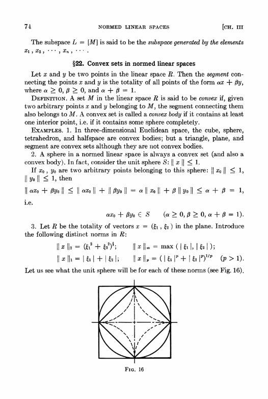
NORMED LINEAR SPACES [CR. III
The subspace L = [M] is said to be the subspace generated by the elements Xl , X2, ••• , X n , ••• •
§22. Convex sets in normed linear spaces
Let X and y be two points in the linear space R. Then the segment connecting the points x and y is the totality of all points of the form ax + {3y, where a ~ 0, {3 ~ 0, and a + {3 = 1.
DEFINITION. A set M in the linear space R is said to be convex if, given two arbitrary points x and y belonging to M, the segment connecting them also belongs to M. A convex set is called a convex body if it contains at least one interior point, i.e. if it contains some sphere completely.
ExAMPLES. 1. In three-dimensional Euclidean space, the cube, sphere, tetrahedron, and halfspace are convex bodies; but a triangle, plane, and segment are convex sets although they are not convex bodies.
2. A sphere in a normed linear space is always a convex set (and also a convex body). In fact, consider the unit sphere S: II x " ::; 1.
If Xo , Yo are two arbitrary points belonging to this sphere: II Xo II ::; 1, II Yo II ::; 1, then
II aXo + {3yo II ::; II aXo II + 1\ {3yo 1\ = a II XO II + {3 1\ Yo 1\ ::; a + {3 1,
I.e.
axo + {3yo E S (a ~ 0, {3 ~ 0, a + (3 = 1).
3. Let R be the totality of vectors x = (~l, ~2 ) in the plane. Introduce the following distinct norms in R:
1\ X 112 = (~/ + ~22)!; 1\ x 1100 = max ( I ~ll, I ~21 ); II x III = I ~l I + I ~21; II x lip = ( I ~l IP + I ~2 IP)l/P (p > 1).
Let us see what the unit sphere will be for each of these norms (see Fig. 16).
FIG. 16

§22] COKVEX SETS IN KORMED LINEAR SPACES 75
In the case II x Ib it is a circle of radius 1, in the case II x II", it is a square with vertices (±1, ±1), in the case II x III it is a square with vertices (0, 1), (1,0), (-1,0), (0, -1). If we consider the unit sphere corresponding to the norm II x lip, and let p increase from 1 to ~, then this" sphere" deforms in a continuous manner from the square corresponding to II x III to the square corresponding to II x II", . Had we set
(1) II x lip = (I ~l IP + I ~2 IP)l/P
for p < 1, then the set II x lip:::; 1 would not have been convex (for example, for p = 2/3 it would be the interior of an astroid). This is another expression of the fact that for p < 1 the "norm" (1) does not satisfy Condition :3 in the definition of a norm.
4. Let us consider a somewhat more complicated example. Let <I> be the set of points x = (6, ~2, ••• , ~n, ... ) in l2 which satisfy the condition
L~~l ~nV :::; 1.
This is a convex set in l2 which is not a convex body. In fact, if x, y E <I> and z = ax + {3y, where a, {3 ~ 0 and a + {3 = ], then by virtue of the Schwarz inequality (Chapter II),
L~=l n2(a~n + {3'r/n)2 = a2 L~=l n2~n2 + 2a{3 L~~l n2~n'r/n + {32 L~~l n2'r/n2
:::; a2 L~=l n2~n2 + 2a{3 (L~=l n2~n2)!(L~=1 n2'r/n2)! + {32 L~=l n2'r/n2
= [a(L n2~n2)l + {3(L n2'r/n2)!]2 :::; (a + {3/ = 1.
We shall show that <I> contains no sphere. <I> is symmetric with respect to the origin of coordinates; hence, if <I> contained some sphere S', it would also contain the sphere S" which is symmetric to S' with respect to the origin. Then <1>, being convex, would contain all segments connecting points of the spheres S' and S", and consequently it would also contain a sphere S of the same radius as that of S', with the center of S at the origin. But if <I> contained some sphere of radius r with center at the origin, then on every ray emanating from zero there would lie a segment belonging entirely to <1>. However, on the ray defined by the vector (1, 1/2, 1/3, ... , l/n, ... ) there obviously is no point except zero which belongs to <1>.
EXERCISES. 1. Prove that the set <I> is compact. Prove that no compact convex set in l2 can be a convex body.
2. Prove that <I> is not contained in any subspace distinct from all of l2 . 3. Prove that the fundamental parallelopiped in l2 (see Example 3, §16)
is a convex set but not a convex body. We shall now establish the following simple properties of convex sets. THEOREM 1. The closure of a convex set is a convex set. Proof. Let M be a convex set, [M] its closure and let x, y be two arbitrary

7{i XORMED LINEAR SPACES [CII. 1ll
points in [M]. Further, let E be an arbitrary positive number. Points a, b can be found in M such that p(a, x) < E and p(b, y) < E. Then p(ax + (Jy, aa + (Jb) < E for arbitrary nonnegative a and (J such that a + (J = 1, and the point aa + (Jb belongs to M since M is convex. Since E > 0 is arbitrary, it follows that ax + (Jy E [M], i. e. [M] is convex also.
THEOREM 2. The intersection of an arbitrary number of convex sets is a convex set.
Proof. Let M = n",.i1f '" , where all M '" are convex sets. Further, let x and y be two arbitrary points in 1If. These points x and y belong to all .i1f '" . Then the segment connecting the points x and y belongs to each M", and consequently it also belongs to M. Thus, M is in fact convex.
Since the intersection of closed sets is always closed, it follows that the intersection of an arbitrary number of closed convex sets is a closed convex set.
Let A. be an arbitrary subset of a normed linear space. We define the convex closure of the set A to be the smallest closed convex set containing A.
The convex closure of any set can obviously be obtained as the intersection of all closed convex sets which contain the given set.
Consider the following important example of convex closure. Let Xl, X2, ... , Xn+l be points in a normed linear space. We shall say that these n + 1 points are in general position if no three of them lie on one straight line, no four of them lie in one plane, and so forth; in general, no k + 1 of these points lie in a subspace of dimension less than k. The convex closure of the points Xl , X2, . . . ,X,,+l which are in general position is called an n-dimensional simplex and the points Xl , X2, ... , X,,+l themselves are called the vertices of the simplex. A zero-dimensional simplex consists of a single point. One-, two-, and three-dimensional simplexes are, respectively, a segment, triangle, tetrahedron.
If the points Xl , X2, ... , X,,+l are in general position, then any k + 1 of them (k < n) also arc in general position and consequently they generate a k-dimensional simplex, called a k-dimensional face of the given n-dimensional simplex. For example, the tetrahedron with the vertices el , e2 , ea ,
e. has four two-dimensional faces defined respectively by the triples of vertices (e2, ea, e.), (el , ea, e4), (el , e2 , e.), (el , e2 , ea); six one-dimensional faces; and four zero-dimensional faces.
THEOREM 3. A simplex with the vertices Xl , X2, ... , X"+1 is the totality of all points which can be represented in the form
(2) ~n+l 1 ,,-,k-l ak = .
Proof. In fact, it is easy to verify that the totality of points of the form (2) represents a closed convex set which contains the points Xl , X2, ... , Xn+1 . On the other hand, every convex set which contains the points Xl, X2 ,
§23j LINEAR FUNCTIONALS 77
... , Xn+l must also contain points of the form (2), and consequently these points form the smallest closed convex set containing the points Xl, X2 , ... ,Xn+l.
§23. Linear functionals
DEFINITION 1. A numerical function f(x) defined on a normed linear space R will be called a functional. A functional f(x) is said to be linear if
f(ax + (3y) = af(x) + (3f(y),
where X, Y E R and a, (3 are arbitrary numbers. A functional f(x) is said to be continuous if for arbitrary E > 0 a 8 > 0
can be found such that the inequality
I f(XI) - f(X2) I < E
holds whenever
II Xl - x211 < 8.
In the sequel we shall consider only continuous functionals (in particular continuous linear functionals) and for brevity we shall omit the word " continuous".
We shall establish some properties of linear functionals which follow almost directly from the definition.
THEOREM 1. If the linear functionalf(x) is continuous at some point Xo E R, then it is continuous everywhere in R.
Proof. In fact, let the linear functional f(x) be continuous at the point X = Xo • This is equivalent to the fact that f(xn ) ~ f(Xo) when x .. ~ Xo •
Further, let Yn ~ y. Then
f(Yn) = f(Yn - Y + Xo + Y - Xo) = f(Yn - Y + xo) + f(y) - f(xo).
But y .. - Y + Xo ~ Xo. Consequently, by assumption, f(Yn - Y + Xo) ~ f(xo). Thus,
f(Yn) ~ f(xo) + f(y) - f(Xo) = f(y)·
A functional f(x) is said to be bounded if there exists a constant N such that
(1) I f(x) I < N II X II for all X E R.
THEOREM 2. For linear functionals the conditions of continuity and boundedness are equivalent.
Proof. We assume that the linear functional f(x) is not bounded. Then for

78 NORMED LINEAR SPACES [CH. III
arbitrary natural number n we can find an element Xn E R such that If(xn ) I > nil Xn II. We shall set Yn = xnl(n II Xn II). Then II Yn II = lin, i.e. y" ~ O. But at the same time
I f(y,,) I = I f(xnln II Xn II) I = (lin II Xn II> I f(xn) I > 1.
COlltlequently, the fUllctional f(x) is not continuous at the point x = O. Now let N be a number which satisfies Condition (1). Then for an arbi
trary sequence ~r" ~ 0 we have:
i.e. f(x) is continuous at the point x = 0 and consequently at all the remaining points also. This completes the proof of the theorem.
DFWINITIO~ 2. The quantity
Ilf Ii = sup {If(x) 1/11 x II; ~v ~ 0)
is called the norm of the linear functional f(x). EXAMPLES OF LINEAR FUNCTIONALS ON VARIOUS SPACES. 1. Let R n be
Euclidean n-space and let a be a fixed nonzero vector in Rn. For arbitrary x E R n we setf(x) = (x, a), where (x, a) is the scalar product of the vectors ;r and a. It is clear that f(x) is a linear functional. In fact,
f(a:c + (jy) = (ax + (jy, a) = a(x, a) + (j(y, a) = af(x) + (jf(y).
Further, by virtue of Schwarz's inequality
(2) If(x) I = I (x, a) I:::; II x 1111 a II·
Consequently, the functional f(x) is bounded and is therefore continuous. From (2) we find
If(x)1/1I;c II :::; II all·
Since the right member of this inequality does not depend on x, we have
sup I f(x) 1/11 x II :::; II a II,
i.e. II f II :::; II a II· But, setting x = a we obtain:
I f(a) I = (a, a) = II a 11 2, i.e. (I f(a) 1I1I a II> = II a II· Therefore II f II = II a II·
If a is zero, then f is the zero linear functional. Hence II f II this case also.
2. The integraJ
I = { x(t) dt
II a II in
§23] LINEAR FUNCTIONAl,!'; 79
(x(t) is a continuous function on [a, b]) represents a linearfullctional on the space era, b]. Its norm equals b - a. In fact,
I I I = I t .l:(t) dt I :s; max I :l:(t) I (b - a),
where equality holds when x = constant. 3. Now let us consider a more general example. Let Yo(t) be a fixed con
tinuous function on fa, b]. We set, for arbitrary function x(t) E era, b],
f(x) = { x(t)yo(t) dt.
This expression represents a linear functional on era, b] because
f(ax + (3y) = t (ax(t) + (3y(t»yo(t) dt
= a t x(t)yo(t) dt + (3 t y(t)yo(t) dt = af(x) + (3f(y)·
This functional is bounded. In fact,
I f(x) I = I t x(t)yo(t) dt I :s; II x II t I yo(t) I dt.
Thus, the functional f(x) is linear and bounded and consequently it is continuous also. It is possible to show that its norm is exactly equal to
t I yo(t) I dt.
4. We now consider on the same space era, b] a linear functional of another type, namely, we set
c5 tox(t) = x(to),
i.e. the value of the functional c5 to for the function x(t) is equal to the mluE' of this function at the fixed point to. This functional is frequently encountered, for example, in quantum mechanics whE're it is usually written in the form
b
c5 tox(t) = L x(t)c5(t - to) dt,
where c5(t) is the "function" equal to zero everywhere except at the point t = 0 and such that its integral equals unity (the Dirac c5-function). The c5-function can be thought of as the limit, in some sense, of a sequence of functions ~n(t) each of which assumes the value zero outside some En-neighborhood (En ---+ 0 as n ---+ 00) of the point f = 0 and such that the integral of the limiting function equals 1.
80 NORMED LINEAR SPACES [CH. III
5. In the space l2 we can define a linear functional as in R n by choosing in l2 some fixed element a = (aI, a2, ... , an, ... ) and setting
(3)
Series (3) converges for arbitrary x E l2 and
(4) I L'::-l xnan I ~ (L'::=l xn 2)1(L'::_1 an2)l = II x 1111 a II. Inequality (4) transforms into the identity L'::=l an2 == L'::-l an2 for
x = a and consequently II f II = II a II. Geometric interpretation of a linear functional. Let f(x) be a linear func
tional on the space R. We shall assume f(x) is not identically zero. The set L, of those elements x in R which satisfy the condition f(x) = 0 form a subspace. In fact, if x, y E L" then
f(ax + (jy) = af(x) + (jf(y) = 0,
Le. ax + (jy E L f • Further, if Xn ~ x and Xn E L" then by virtue of the continuity of the functional f,
f(x) = limn-+oof(xn) = o. DEFINITION 3. We say that the subspace L of the Banach space R has
index (or deficiency) s if: 1) R contains s linearly independent elements Xl , X2, ... , x. which do not belong to L with the property that every element x E R can be represented in the form
y E L;
and 2) it is impossible to find a smaller number of elements Xi which possess the indicated properties.
In the case of a finite-dimensional space R the index plus the dimension of the subspace L is equal to the dimension of the whole space.
THEOREM 3. Letf(x) ~ 0 be a given functional. The subspace L, has index equal to unity, i.e. an arbitrary element y E R can be represented in the form
(5) y = XXo + x,
where x E L" Xo ~ L, . Proof. Since Xo ~ L" we have f(:to) ¢ o. If we set X = f(y)/f(xo) and
x = y - {f(y)/f(xo) }xo, then y = XXo + x, where
f(x) = fey) - (f(y)/f(xo))f(xo) = o. If the element Xo is fixed, then the element y can be represented in the
form (5) uniquely. This is easily proved by assuming the contrary. In fact, let
y = XXo + x,
y = X'xo + X'j

§24] THE CONJUGATE SPACE 81
then
(>' - >.')xo = (x' - x).
If >. - >" = 0, then obviously, x - x' = O. But if >. - >" ~ 0, then Xo = (x' - x)/(>' - >") E L, , which contradicts the condition that Xo Ef L,.
Conversely, given a subspace L of R of index 1, L defines a continuous linear functional f which vanishes precisely on L. Indeed, let Xo Ef L. Then for any x E R, x = y + >,xo , with y E L, XO Ef L. Letf(x) = >.. It is easily seen that f satisfies the above requirements. If f, g are two such linear functionals defined by L, then f(x) = ag(x) for all x E R, a a scalar. This follows because the index of L in R is 1.
We shall now consider the totality "AI, of elements in R which satisfy the condition f(x) = 1. "AI, can be represented in the form "AI, = L, + Xo, where Xo is a fixed element such that f(xo) = 1 and L, is the totality of elements which satisfy the condition f(x) = O. In analogy with the finitedimensional case it is natural to call "AI, a hyperplane in the space R. It is easy to verify that the hyperplanesf(x) = 1 and Ip(x) = 1 coincide if, and only if, the functionals f and Ip coincide. Thus, it is possible to establish a one-to-one correspondence between all functionals defined on R and all hyperplanes in R which do not pass through the origin of coordinates.
We shall now find the distance from the hyperplane f(x) = 1 to the origin. It is equal to
d = inf {II x II; f(x) = 1}.
For all x such that f(x) = 1 we have
1 ~ IIf 1111 x II, i.e. II x II ~ 1/11 f II ;
therefore d > 1/11 f II. Further, since for arbitrary E > 0 an element x satisfying the condition f(x) = 1 can be found such that
1 > (II f II - e) II X II, it follows that
d = inf {II x II < 1/(llfll - E);f(x) = II. Consequently,
d = 1/11 f II,
i.e. the norm of the linear functional f(x) equals the reciprocal of the magnitude of the distance of the hyperplane f(x) = 1 from the origin of coordinates.
§24. The conjugate space
It is possible to define the operations of addition and mUltiplication by a scalar for linear functionals. Let fl and f2 be two linear functionals on a

82 NORMED LINEAR SPACES [CH. III
nonned linear space R. Their sum is a linear functionp.l f = fl + f2 such that f(x) = fl(X) + /2(x) for arbitrary x E R.
The product of a linear functionalfl by a number a is a functionalf = afl such that
f(x) = a/I(x)
for arbitrary x E R. It is easy to verify that the operations of addition and mUltiplication by
a scalar of functionals so defined satisfy all the axioms of a linear space. Moreover, the definition we gave above of the norm of a linear functional satisfies all the requirements found in the definition of a nonned linear space. In fact,
1) II f II > 0 for arbitrary f t= 0,
2) II af II = I a I II f II, 3) II fl + f2 II = sup {I fl(X) + /2(x) 1/11 x II}
~ sup {(I /I(x) I + 1/2(x) Dill X II} ~ sup {I/I(x) 1111 x II} + sup {1/2(x) 1111 X II} = II /I II + II /2 II·
Thus, the totality of all linear functionals on a nonned space R itself represents a normed linear space; it is called the conjugate space of Rand is denoted by R.
THEOREM 1. The conjugate space is always complete. Proof. Let {f .. } be a fundamental sequence of linear functionals. By the
definition of a fundamental sequence, for every E > 0 there exists an N such that II fn - fm II < E for all n, m > N. Then for arbitrary x E R,
I fn(x) - fm(x) I ~ II fn - fm II II x II < E II x II, i.e. for arbitrary x E R the numerical sequence fn(x) converges.
If we set
f(x) = limn .... f,,(x),
then f(x) represents a linear functional. In fact,
1) f(ax + ~y) = lim ...... fn(ax + ~y) = limn .... [afn(x) + ~fn(Y)] = af(x) + ~f(y).
2) Choose N so that II fn - fn+p II < 1 for all n > N. Then
II fn+p II < "f" " + 1
for all p. Consequently, I f,,+p(x) I ~ (II f .. II + 1) II x II·
§2-!] THE CONJUGATE SPACg 83
Passing to the limit as p ~ 00, we obtain
limp _ oo I fn+p(x) I = I f(x) I :::; (II fn II + 1) II x II,
i.e. the functional f(x) is bounded. We shall now prove that the functional f is the limit of the sequence fl , f2, ... ,fn, .... By the definition of the norm, for every E > 0 there exists an element x. such that
II fn - f II :::; {(I fn(x.) - f(x.) Dill x. III + E/2
= I fn(x./II x. II) - f(x./1I x. ID I + E/2;
since
f(x./1I x. ID = limn_oofn(x./1I x. II), it is possible to find an nO(E) such that for n > no
I fn(x./1I x. ID - f(x./1I x. ID I < E/2,
so that for n > no the inequality
IIfn - f II < E
is fulfilled. This completes the proof of the theorem. Let us emphasize once more that this theorem is valid independently of
whether the initial space R is complete or not. EXAMPLES. 1. Let the space E be finite-dimensional with basis el , e2, ... ,
en . Then the functional f(x) is expressible in the form
(1)
where x = Li-l Xiei and h = f(ei). Thus, the functional is defined by the n numbers II, ... ,fn which are
the values of f on the basis vectors. The space which is the conjugate of the finite-dimensional space is also fir"iite-dimellsional and has the same dimension.
The explicit form assumed by the norm in the conjugate space depends on the choice of norm in E.
a) Let II x II = (L xl)!. We have already shown that then
II f II = (L fl)t, i.e. the conjugate of an Euclidean space is itself Euclidean.
b) Let II x II = sup. I Xi I. Then
I f(x) I = I Lf.Xi I :::; (L I fi D sup. I Xi 1,= (L I fi D II x II·
From this it follows that
Ilfll:::; Llhl·

84 NORMED LINEAR SPACES
The norm II I II cannot be less than L I Ii I since if we set
r +1 if Ii > 0,
Xi = 1-1 if Ii < 0,
l 0 if fi = 0,
then the following equ,ality is vaJid:
II(x) I = L I Ii I = (L Ifi [) II X II·
[CH. III
c) If II:r II = (L I Xi nl/p, p > 1, then II I II = (L I Ii Iq)l/q, where
lip + 11q = 1. This follows from the Holder inequality
I L Iixi I ::; (L I Xi IP)I/P(L I Ii Iq)l/q and from the fact that the equality sign is attained [for Ii = (sgn Xi) (Xiy-Ij.
2. Let us consider the space c consisting of sequences X = (Xl, X2, ••• ,
;:fn , ••• ) which are such that Xn -+ 0 as n -+ 00, where II X II = supn Xn •
If a functional in the space c is expressible by means of the formula
(2)
then it has norm
II I II = L~l I Ji I· The inequality II I II ::; Li:.l I Ii I is obvious. On the other hand, if
L~l I Ii I = 0;, then for every ~ > 0 it is possible to find an N such that Lf=l I Ii I > a - ~.
We now set
Xn =
Then
+1 if In > O} -1 ~f In < 0 n::; N.
o If In = 0
Oifn>N
II(x) I = L~=l I In I > a - ~,
whence it follows that II I II = a. We shall prove that all functionals in the space c have the form (2).
We shall set
en = (0, 0, ... , 1, 0, ... ),
i.e. en denotes the sequence in which the n-th entry is unity and the remaining are zeros.

§24] THE CONJUGATE SPACE 85
Let the functional f(x) be given; we denote fee,,) by j" . If
(3) x = (Xl, X2, ... , X" , 0, ... ),
then
X = Xlel + X~2 + '" + x"e" and f(x) = }2i=diXi.
The sum }2':=1 I f" I is < 00 for every bounded linear functional. If }2':-1 I f" I were = 00, then for every H it would be possible to find an N such that
}2!=1 I f" I > H.
We construct the element X in the following way:
1 iff" > O} -1 if f" < 0 n::; N.
x" = Oiff=O
Oifn>N
The norm of such an element is equal to unity, and
I f(x) I = }2f-d''Xi = }2f=1 I fi I > H = H II X II, which contradicts the assumption concerning the boundedness of the functional.
The set of elements of the form (3) is everywhere dense in the space c. Therefore the continuous linear functional is uniquely defined by its values on this set. Thus, for every X
f(x) = }2~-1 fiX; .
The space which is conjugate to the space c consists of sequences
(ft, h, ... , f", ... ) satisfying the condition }2~1 I f" I < 00.
3. Let the space consist of sequences
x = (Xl, X2, .. , , x,,, ... ), }2':'..1 I Xi I < 00
with norm II X II = }2':=1 I x" I· It can be proved that the space conjugate to this space is the space of
bounded sequences
f = (fl, h, ... ,f", ... )
with norm II f II = sup" I f" I· In all the examples of finite-dimensional spaces introduced above, the
space which is conjugate to the conjugate space coincides with the initial

80 ~OHMED LINEAR SPACES [c1I. III
spacc. This is ahmys so in the finite-dimensional case. However, as Examples 2 and :3 show, in the infinite-dimensional case the space conjugate to the conjugate space may not coincide with the ,initial space.
We consider ('ases w}](,11 this coincidence holds also in infinite-dimensional space.
4. The spaec 12 consists of sequences
, xn , •.. ),
\yith L~I :/.'/ < co and norm 11 x II = (L~=I :r/)!. All functiona!s in the spaee 12 have t.he form
f(x) = L~=d;x,.
We shall prove this assertion. To each functional there is set into correspondence the sequence fl , f2 ,
... , fn, ... of its values on the elements CI, C2, ••• , en, ... defined exactly as in Example 2, above.
If the functional is bounded, then L~lf/ < OC. We shalI assume the contrary, i.e. we shall assume that for every H t.here exists an N such that
Lf=lf/ = U ~ H.
If \ye apply the functional under consideratioll to the element
.r = (fr, f2, ... ,fN , 0, ... ), Ilx I! = Td ~, ,
we obt.ain
f(x) = Lf=lfl = u ~ HI II x II,
contrary to the assumption that the functional is bounded. Since the functional f is linear, its values on the elements of the form
x = (;rl, X2, .•• , ;rn , 0, ... ) are easily found; on all other elements of the space the values of f are found from continuity considerat.ions and we always haY('
f(x) = L~If,.:r;.
The norm of the functional f equals (L~lfN. This is established with the aid of the Schwarz inequality .
. 1. The space Ip is the space of alI sequences of the form
:1' = (XI, X2, ... , X n , ••• ), (L~I X/)I/P < co, II x II = (L~=I X/)I/P.
The conjugate space of lp is the space lq ,where l/p + l/q = 1. The proof is analogous to the preceding proof. Hint: Use HOlder's inequality.
§26. Extension of linear functionals
THEOREM (HAHK-BANACH). Every linear functional f(x) defined on a linear subspace G of a normed linear space E can be extended to the entire
§25] EXTENSION OF LINEAR FUNCTIONALS 87
space with preservation of norm, i.e. it is possible to construct a linear functional F(x) such that
1) F(x) = f(x), x E G,
2) II F /IE = II f 110 .
Proof. The theorem will be proved for a separable space E, although in actuality it is valid also in spaces which are not separable.
First, we shall extend the functional to the linear subspace G1 obtained by adding to G some element Xo EE G. An arbitrary element of this subspace is uniquely representable in the form
y = txo + x,
If the functional sought exists, then
x E G.
F(y) = tF(xo) + f(x)
or, if we :;et -F(xo) = c, then F(y) = f(x) - ct. In order that the norm of the functional be not increased when it is
continued it is necessary to find a c such that the inequality
(1) If(x) - ct I :::; I! f II II x + txo II be fulfilled for all x E G.
If we denote the element xlt by z Cz E G), the inequality (1) can be rewritten
IfCz) - c I :::; II f II II z + Xo II·
This inequality is equivalent to the following inequalities:
-Ilf 1111 z + XO II :::; fez) - c :::; Ilf IIII z + Xo II,
or, what amounts to the same thing,
fez) + I! f I! II z + Xo II 2: c 2: fCz) - Ilf II /I z + Xo II,
for all z E G. We shall prove that such a number c always exists. To do this we shall show that for arbitrary elements z', z" E G we always have
(2) f(z") + II f II II z" + Xo II 2: fez') - II f II II z' + Xo II· But this follows directly from the obvious inequality
fez') - f(z") :::; II f II II z' - z" II = II f II II z' + Xo - (z" + xo) II ~ II f II II z' + Xo II + II filii z" + Xo /I.
We introduce the notation:
c' = inf lJ(z) + II f II II z + Xo II; z E GJ,
c" = sup lJ(z) - /I f II II z + Xo II; z E GJ.
88 NORMED LINEAR SPACES [CR. III
It follows from inequality (2) that clf ::; c/. We take an arbitrary c such that clf ::; c ::; c/. We set
Fl(x) = f(x) - ct
for the elements of the subspace Gl = {G U xo} . We obtain the linear functional Fl , where II Fl II ,= II f II·
The separable space E contains a denumerable everywhere dense set x, • X2. ••• , xn , ••• • We shall construct the linear subspaces
Gl = {G U xo},
G2 = {Gl U xd,
and define the functional F on them as follows: we construct functionals F n which coincide with F n-l on Gn- l and which have norm equal to II f II. Thus, we obtain the functional F defined on a set which is everywhere dense in E. At the remaining points of E the functional is defined by continuity: if x = limn ..... Xn , then F(x) = limn ..... F(xn). The inequality I F(x) I ::; II filII x II is valid since
I F(x) I = limn ..... I F(xn) I ::; limn ..... II filii Xn II = II f 1111 x II· This completes the proof of the theorem on the extension of a functional. COROLLARY. Let Xo be an arbitrary nonzero element in R and let M be an
arbitrary positive number. Then there exists a linear functional f(x) in R such that
II f II = M and f(xo) = II f II II Xo II· In fact, if we set f(txo) = tM II Xo II, we obtain a linear functional with norm equal to M which is defined on the one-dimensional subspace of elements of the form txo and then, by the Hahn-Banach theorem, we can extend it to all of R without increasing the norm. The geometric interpretation of this fact is the following: in a Banach space through every point Xo there can be drawn a hyperplane which is tangent to the sphere II x II = II Xo II.
§26. The second conjugate space
Inasmuch as the totality R of linear functionals on a normed linear space R itself represents a normed linear space it is possible to speak of the space It of linear functionals on R, i.e. of the second conjugate space with respect to R, and so forth. We note first of all that every element in R defines a linear functional in R. In fact, let
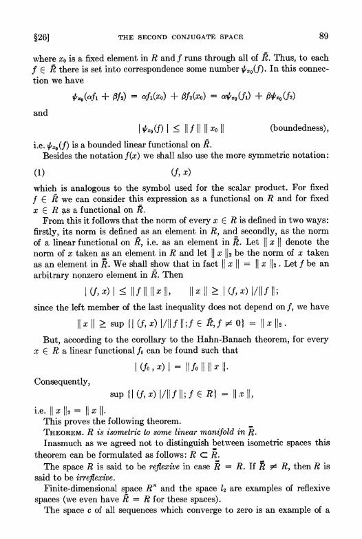
§26] THE SECOND CONJUGATE SPACE 89
where Xo is a fixed element in Rand f runs through all of R. Thus, to each fER there is set into correspondence some number 1/;zo(f). In this connection we have
and
l1/;zo (f) I :::; II f II II Xo II (boundedness) ,
i.e.1/;xo(f) is a bounded linear functional on R. Besides the notation f(x) we shall also use the more symmetric notation:
(1) (f, x)
which is analogous to the symbol used for the scalar product. For fixed fER we can consider this expression as a functional on R and for fixed x E R :;tS a functional on R.
From this it follows that the norm of every x E R is defined in two ways: firstly, its norm is defined as an element in R, and secondly, as the norm of a linear functional on R, i.e. as an element in R. Let II x II denote the norm of x taken as an element in R and let II x 112 be the norm of x taken as an element in R. We shall show that in fact II x II = II x 112. Let f be an arbitrary nonzero element in R. Then
I (f, x) I :::; II filii x II, II x II ~ I (f, x) 1111 f II;
since the left member of the last inequality does not depend on f, we have
II x II ~ sup II (f, x) 1/IIf II;f E R;f ~ O} = II X 112.
But, according to the corollary to the Hahn-Banach theorem, for every x ERa linear functional fo can be found such that
I (fo, x) I = II fo II II x II·
Consequently,
sup II (j, x) 1/IIf II; fER} II x II, i.e·llxI12= Ilxll·
This proves the following theorem. THEOREM. R is isometric to some linear manifold in'R. Inasmuch as we agreed not to distinguish between isometric spaces this
theorem can be formulated as follows: R c R. The space R is said to be reflexive in case R = R. If R ~ R, then R is
said to be irreflexive. Finite-dimensional space R n and the space l2 are examples of reflexive
spaces (we even have R = R for these spaces). The space c of all sequences which converge to zero is an example of a

90 XORMED LINEAR SPACES [CH. III
complete irreflexive space. In fact, above (§24, Examples 2 and 3) we proved that the conjugate space of the space c is the space l of numerical sequences (Xl, X2, '" , Xn , ... ) which satisfy the condition L:~~l I Xn I < 00, to which in turn the space m of all bounded sequences is conjugate. The spaces c and m are not isometric. This follows from the fact that c is separable and m is not. Thus, c is irreflexive.
The space C[a, b] of continuous functions on a closed interval [a, b] is also irreflexive. However, we shall not stop to prove this assertion. (The following stronger assertion can also be proved: No normed linear space exists for which C[a, b] is the conjugate space.)
A. I. Plessner established that for an arbitrary normed space R there exist only two possibilities: either the space R is reflexive, i.e. R = R R"" = ... . R = Re = ... . or the spaces R R R= '" are all distinct , , , , , .
The space lp(p > 1) is an example of a reflexive space (since lp = lq, where lip + 1/q = 1, we have lp = lq = lp).
§27. Weak convergence
The concept of so-called weak convergence of elements in a normed linear space plays an important role in many questions of analysis.
DEFINITION. A sequence {xnl of elements in a normed linear space R converges weakly to the element X if
1) The norms of the elements Xn are uniformly bounded: II Xn II :::; lVI, and
2) f(xn) -+ f(x) for every fER. (It can be shown that Condition 1 follows from 2; we shall not carry out this proof.)
Condition 2 can be weakened slightly; namely, the following theorem is true.
THEOREM 1. The sequence I Xn I converges weakly to the element x if 1) II Xn 11 :::; lVI, and 2) f(xn) -+ f(x) for every .f E ~,where ~ is a set whose lineal' hull is
everywhere dense in R. Proof. It follows from the conditions of the theorem and the definition
of a linear functional that if tp is a linear combination of elements in ~ then tp(Xn) -+ tp(x).
N ow let tp be an arbitrary linear functional on R and let {tpk I be a sequence of functionals which converges to tp, each of which is a linear combination of elements in ~. We shall show that tp(xn) -+ tp(x). Let M be such that II Xn II :::; M (n = 1,2, ... ) and II X II :::; M.
Let us evaluate the difference Itp(xn) - tp(x) I. Since tpk -+ tp, given an arbitrary E > 0 a K can be found such that for an k > K,
IItp - tpk 11 < E;
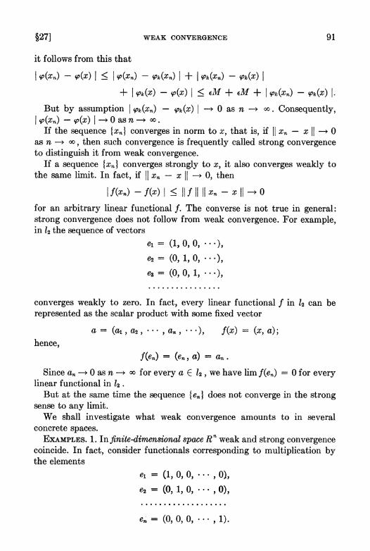
§27] WEAK CONVERGENCE 91
it follows from this that
I 'P(xn) - 'P(x) I ~ I 'P(xn) - 'Pk(Xn) I + I 'Pk(Xn) - 'Pk(X) I + I 'Pk(X) - 'P(X) I ~ EM + EM + I 'Pk(Xn) - 'Pk(X) I·
But by assumption I 'Pk(Xn) - 'Pk(X) I ~ ° as n ~ 0Ci. Consequently, I 'P(xn) - 'P(x) I ~ ° as n ~ 0Ci.
If the sequence {Xn} converges in norm to x, that is, if II Xn - x II ~ ° as n ~ 0Ci, then such convergence is frequently called strong convergence to distinguish it from weak convergence.
If a sequence {Xn} converges strongly to x, it also converges weakly to the same limit. In fact, if II Xn - x II ~ 0, then
I f(xn) - f(x) I ~ II filii Xn - x II ~ ° for an arbitrary linear functional f. The converse is not true in general: strong convergence does not follow from weak convergence. For example, in l2 the sequence of vectors
el = (1, 0, 0, ... ),
e2 = (0, 1, 0, ... ),
ea = (0, 0, 1, ... ),
converges weakly to zero. In fact, every linear functional f in l2 can be represented as the scalar product with some fixed vector
a = (al' ~, ... , an, ... ), f(x) = (x, a);
hence,
Since an ~ ° as n ~ 0Ci for every a E l2, we have lim f(en) = ° for every linear functional in l2 .
But at the same time the sequence {en} does not converge in the strong sense to any limit.
We shall investigate what weak convergence amounts to in several concrete spaces.
EXAMPLES. 1. Infinite-dimensional space R n weak and strong convergence coincide. In fact, consider functionals corresponding to multiplication by the elements
el (1, 0, 0, ... , 0),
e2 (0, 1, 0, ... , 0),
e'; = (0, 0, 0, ... , 1).

92 NORMED LINEAR SPACES [CH. III
If I Xk) converges weakly to X, then
(Xk, ei) = Xk (i) ~ X(i) (i = 1, 2, ... , n),
i.e. the first coordinates of the vectors Xk tend to the first coordinate of the vector x, their second coordinates tend to the second coordinate of the vector x, and so forth. But then
( ) I ~n «i) (i»)2)t 0 p Xk, X = L.,i-l Xk - X ~,
i.e. IXk) converges strongly to x. Since strong convergence always implies' weak convergence, our assertion is proved.
2. Weak convergence in l2. Here we can take for the set A, linear combinations of whose elements are everywhere dense in l2, the totality of vectors
el = (1, 0, 0, ... ),
e2 = (0, 1, 0, ... ),
e3 = (0, 0, 1, ... ),
If x = (~l, ~, ... , ~n, ... ) is an arbitrary vector in l2 , then the values assumed at x by the corresponding linear functionals are equal to (x, en) = ~'" i.e. to the coordinates of the vector x. Consequently, weak convergence of the sequence Ix,,) in l2 means that the numerical sequence of the k-th coordinates of these vectors (k = 1,2, ... ) converges. We saw above that this convergence does not coincide with strong convergence in l2 •
3. Weak convergence in the space of continuous functions. Let C[a, b] be the space of continuous functions defined on the closed interval [a, b]. It ('an be shown that the totality A of all linear functionals 8to , each of which is defined as the value of the function at some fixed point to (see Example 4, §23) satisfies the conditions of Theorem 1, i.e. linear combinations of these functionals are everywhere dense in era, b]. For each such functional 8to , the condition 8tox,,(t) ~ 8tox(t) is equivalent to the condition Xn(tO) ~ x(to).
Thus, weak convergence of a sequence of continuous functions means that this sequence is a) uniformly bounded and b) convergent at every point.
It is clear that this convergence does not coincide with convergence in norm in C[a, b], i.e. it does not coincide with uniform convergence of continuous functions. (Give a suitable example!)
§28. Weak convergence of linear functionals
We can introduce the concept of weak convergence of linear functionals as analogous to the concept of weak convergence of elements of a normed linear space R.

§28] WK-I.K CO)<VERGENCl'J OF LINEAR FU)<CTIONALS 93
DEFINITION. A sequence Ifn} of linear functionals converges weakly to the linear functional f if
1) "fn" are uniformly bounded; i.e. "fn II :::; M, and 2) fn(x) ~ f(x) for every element x E R.
(This is usually called weak* convergence.-Trans.) 'Veak convergence of linear functionals possesses properties which are
analogous to properties stated above of weak convergence of elements, namely strong convergence (i.e. convergence in norm) of linear functionals implies their weak convergence, and it is sufficient to require the fulfillment of the condition fn(x) ~ f(x) not of all x E R, but only for a set of elements linear combinations of which are everywhere dense in R.
We shall consider one important example of weak convergence of linear functionals. Above (§23, Example 4), we spoke of the fact that the "a-function", i.e. the functional on era, b], which assigns to every continuous function its value at the point zero, can "in some sense" be considered as the limit of "ordinary" functions, each of which assumes the value zero outside some small neighborhood of zero and has an integral equal to 1. [We assume that the point t = 0 belongs to the interval (a, b). Of course, one can take any other point instead of t = 0.] Now we can state this assertion precisely. Let {'Pn(t)} be a sequence of continuous functions satisfying the following conditions:
(1) 1) 'Pn(t) = 0 for I t I > lin,
2) t 'Pn(t) dt = 1.
Then for an arbitrary continuous function x(t) defined on the closed interval [a, b], we have
Ib I1/n 'Pn(t)X(t) dt = 'Pn(t)X(t) dt ~ x(O) as n ~ 00.
a -lin
In fact, by the mean-value theorem,
11/" llln 'Pn(t)x(t) dt = X(~n) 'P,,(t) dt = X(~n),
-lIn -lin -lin :::;~" :::; lin;
when n ~ 00, ~n ~ 0 and x(~n) ~ x(O). The expression
t 'Pn(t)X(t) dt
represents a linear functional on the space of continuous functions. Thus, the result we obtained can be formulated as follows: the a-function is the limit of the sequence (1) in the sense of weak convergence of linear functionals.

94 XORMED LIXEAR SP.\CES [CH. III
The following theorem plays an important role in various applications of the concept of weak convergence of linear functionals.
ThEOREM 1. If the normed linear space R is separable, then an arbitrary bounded sequence of linear funcUonols on R ronta-ins a weakly con vl'rgen f sUbsequence.
Proof. Choose in R a denumerable everywhere dense set
{Xl , X2, ... , X n , ••• }.
If {fn} is a bounded (in norm) sequence of linear functionals on R, then
fl(Xl), f2(Xl), ... , fn(Xl), ...
is a bounded numerical sequence. Therefore we can select from {fn} a subsequence
J/, fl, ... , fn',
such that the numerical sequence
J/(xl),N(xl),
converges. Furthermore, from the subsequence {fn'} we can select a subsequence
such that
fl"(x2),N'(x2), ...
converges, and so forth. Thus, we obtain a system of sequences
f/, fl, ... , tn', "',
each 01 which is a subsequence of the one preceding. Then taking the "di-agonal" subsequence fl', f2", fa"', ... , we obtain a sequence of linear func-tionals such that J/(xn), f2"(Xn), ... converges for all n. But then J/(x), fl'(x), ... also converges for arbitrary x E R. This completes the proof of the theorem.
The last theorem suggests the following question. Is it possible in the space fl., conjugate to a separable space, to int.roduce a metric so that the bounded subsets of the space fl. become compact with respect to this new metric? In other words, is it possible to introduce a metric in R so that convergence in the sense of this metric in fl. coincides with weak convergence of elements in fl. considered as linear functionals. Such a metric can in fact be introduced in fl..
Let {x n } be a denumerable everywhere dense set in R. Set
(2) p(fl , M = L'::=l I fl(Xn) - MXn) 1/2n II :l~n II

§29] LINEAR OPERATORS 95
for any two elements f1 ,!2 E R. This series converges since its n-th term does not exceed (II h II + II f211)/2n. The quantity (2) possesses all the properties of a distance. In fact, the first two axioms are obviously satisfied. We shall verify the triangle axiom.
Since
I h(xn) - fa(xn) I = I f1(X n) - Nxn ) + f2(Xn ) - fa(x n) I ~ I f1(Xn) - f2(Xn ) I + I !2(xn) - fa(xn) I,
we have
P(f1 ,fa) ~ p(f1 ,f2) + p(f2, fa).
Direct verification shows that convergence in the sense of this metric is in fact equivalent to weak convergence in R.
Now Theorem 1 can be formulated in the following manner. THEOREM 1'. In a space R, which is the conjugate of a separahle space,
with metric (2), every bounded subset is compact.
§29. Linear operators
1. Dejinition of a linear operator. Boundedness and continuity. Let Rand R' be two Banach spaces whose elements are denoted respec
tively by x and y. Let a rule be given according to which to each x in some set X ~ R there is assigned some element y in the space R'. Then we say t.hat an operator y = Ax with range of values in R' has been defined on the set X.
DEFINITION 1. An operator A is said to be linear if the equality
A (a1x1 + a2X2) = a1Ax1 + a~x2 is satisfied for any two elements Xl , X2 E X and arbitrary real numbers a1, a2.
DEFINITION 2. An operator A is said to be bounded if there exists a constant M such that
II A x II ~ M II x II for all x E X.
DEFINITON 3. An operator A is said to be continuous if for arbitrary E > 0 there exists a number ~ > 0 such that the inequality
II x' - x" liB < ~ (x', x" E X)
implies that
II Ax' - Ax" liB' < E.
Only linear operators will be considered in the sequel. If the space R' is the real line, the operator y = A (x) is a functional, and the formulated

96 NORMED LINEAR SPACES [CR. III
definitions of linearity, continuity and boundedness go over into the corresponding definitions introduced in §23 for functionals.
The following theorem is a generalization of Theorem 1, §23. THEoREM 1. Continuity is equivalent to boundedness for a linear operator. Proof. 1. Assume the operator A is bounded. The inequality II x' - x" II <
~ implies that
(1) II Ax' - Ax" II = II A (x' - x") II :::; M II x' - x" II :::; M~, where M is the constant occurring in the definition of boundedness. If we take ~ < ElM, inequality (1) yields II Ax' - Ax" II < E, i.e. the operator A is continuous.
2. Assume now that the operato~ A is continuous. We shall prove that A is bounded by contradiction. We assume that A is not bounded. Then there exists a sequence
(2) Xl , X2, '" , x"' ...
such that
II Ax" II > n II x" II· Set z" = x1./n II x" II; it is obvious that II z" II
n ~ 00. Consider the sequence
Az .. = Ax .. ln II x" II
lin, i.e. z" ~ 0 as
which is the map of the sequence {z,,} under A. The norm of each element Az" is not less than 1:
II Az" II = II Ax .. IIln II x" II ~ n II x" III nil x" II = 1.
Since for every linear operator, A (0) = 0, and lim" ... ,. z .. = 0, we obtain a contradiction of our hypothesis that the operator is continuous. Consequently, the operator A must be bounded.
ExAMPLE. The general form of a linear operator mapping a finite-dimensional space into a finite-dimensional space. Given an n-dimensional space R" with basis el , e2, .. , , e" , every point of this space can be represented in the form x = Ei-l x.e •.
A linear operator A maps R" into the finite-dimensional space R m with the basis el', el, .. , , em'.
Let us consider the representation with respect to this basis of the images of the basis vectors of the space R":
Aei = Ei!-l aije/.
Now let y = Ax,
y = Ax = Ei-l x.Aei = Ei-l Xi Ei!-l aije/ = Ei!-l dje/,

§29] LINEAR OPERATORS 97
where
(3)
It is clear from formula (3) that to determine the operator A it is sufficient to give the coefficient matrix with entries aij •
A linear operator cannot map a finite-dimensional space into a space of greater dimension since all linear relations among the elements are preserved for their images.
2. Norm of an operator. Sum and product of operator8. Product of an operator by a 8calar.
DEFINITION 4. Let A be a bounded linear operator. This means that there exist numbers M such that
(4) II Ax II < M IIx II for all x E X. The norm II A II of the operator A is the greatest lower bound of the numbers M which satisfy condition (4). It follows from the definition of the norm of an operator that II Ax II ::; II A II II x II. But if M < II A II, then there exists an element x such that II Ax II > M II xii.
ThEOREM 2. If A i8 an arbitrary linear operator, then
IIAII = sup {IIAxll; IIxll = I} = sup {IiAx II/II x II; IIxll ¢ OJ.
Proof. Introduce the notation
a = sup {II Ax II; IIxll = I} = sup {II Ax II/II x II; IIxll ¢ OJ.
We shall first prove that II A II ~ a.Sincea = sup{ II Ax II/!Ix II; Ilx II ¢ OJ, for arbitrary E > 0 there exists an element Xl not zero such that II AXI II/II Xl II > a - E or II AXI II > (a - E) II Xl II, which implies that a - E < II A II and hence that II A II ~ a because E is arbitrary.
The inequality cannot hold. In fact, if we let II A II - a = E, then a < II A II - E/2. But this implies that the following inequalities hold for an arbitrary point x:
II Ax II/II x II ::; a < II A II - E/2,
or
II Ax II ::; (II A II - E/2) II x II, i.e. II A II is not the greatest lower bound of those M for which II Ax II ::; M II x II. It is clear from this contradiction that II A II = a.
In the sequel we shall make use of the above expression for the norm of an operator as equivalent to the original definition of the norm.
DEFINITION 5. Let, Al and A2 be two given continuous linear operators which transform the Banach space E into the Banach space E I . The 8um
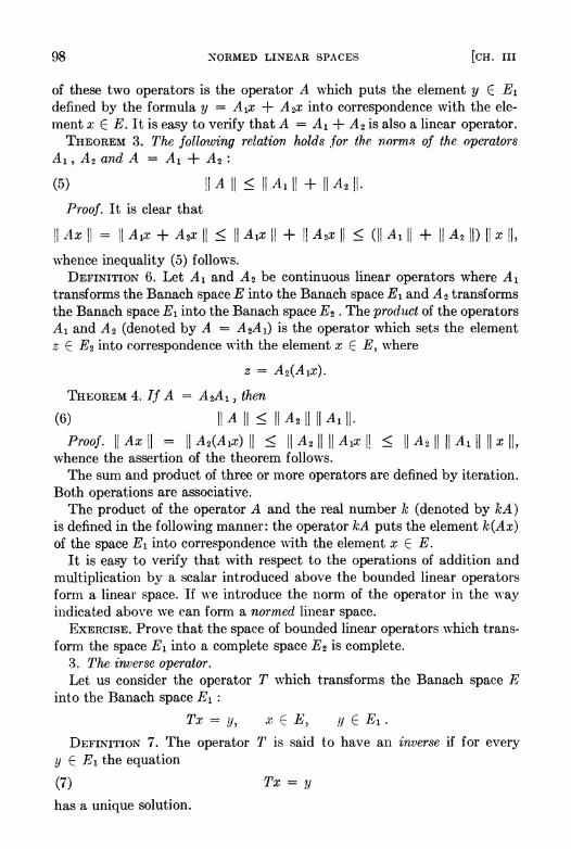
98 XORMED LINEAR SPACES [CH. III
of these two operators is the operator A which puts the element y E E1 defined by the formula y = A 1x + A 2x into correspondence with the element x E E. It is easy to verify that A = A1 + A2 is also a linear operator.
THEOREM 3. The following relation holds for the norm,.~ of the operators A1, A2 and A A1 + A2 :
(5)
Proof. It is clear that
II Ax II = II A 1x + A2X II ~ II A 1x II + I! A 2x II ~ (II A1 II + II A2 II) II x II, whence inequality (5) follows.
DEFINITION 6. Let A1 and A2 be continuous linear operators where A1 transforms the Banach space E into the Banach space E1 and A2 transforms the Banach space E1 into the Banach space E2 . The product of the operators A1 and A2 (denoted by A = A 2A1) is the operator which sets the element z E E2 into correspondence with the element x E E, where
z = A 2(A 1x).
l1moREM 4. l.f A = A~l. then
(6) II A II ~ II A2 1111 A1 II· Proof. II Ax II = II A2(A 1x) II ~ II A21111 A1x I! ~ II A2 1111 A1 1111 x II.
whence the assertion of the theorem follows. The sum and product of three or more operators are defined by iteration.
Both operations are associative. The product of the operator A and the real number k (denoted by kA)
is defined in the following manner: the operator kA puts the element k(Ax) of the space E1 into correspondence with the element x E E.
It is easy to verify that with respect to the operations of addition and multiplication by a scalar introduced above the bounded linear operators form a linear space. If we introduce the norm of the operator in the way indicated above we can form a normed linear space.
EXERCISE. Prove that the space of bounded linear operators which transform the space E1 into a complete space E2 is complete.
3. The inverse operator. Let us consider the operator T which transforms the Banach space E
into the Banach space E1 :
Tx = y, x E E, !J E E1 .
DEFINITION 7. The operator T is said to have an inverse if for every y E E1 the equation
(7) Tx = 1/
has a unique solution.

§29] LINEAR OPERATORS 99
To each Y E El we can put into correspondence the solution of equation (7). The operator which realizes this correspondence is said to be the inverse of T and is denoted by T- l •
THEOREM 5. The operator T- l which is the inverse of the linear operator l' is also linear.
Proof. To prove the linearity of 1'-1 it is sufficient to verify that the equality
1'-1(alYI + a2Y2) = aIT-IYl + a21'- IY2
is valid. Denote 1'Xl by Yl and TX2 by Y2 . Since T is linear, we have
(8)
By the definition of the inverse operator,
whence, multiplying these equations by al and a2 respectively, and adding, we obtain:
aIT-IYl + a2T-IY2 = alXl + a2X2 .
On the other hand, from (8) and from the definition of the inverse operator it follows that
alXl + a2X2 = T-l(al Yl + a2Y2)
which together with the preceding equalities yields
1'1(alYI + a2Y2) = aIT-IYl + a2T-IY2 .
THEOREM 6. If T is a bounded linear operator whose inverse T-l exists, then T-l is bounded.
We shall need the following two lemmas in the proof of this theorem. LEMMA 1. Let M be an everywhere dense set in the Banach space E.
Then an arbitrary element Y E E, Y ~ 0, can be developed in the series
Y = Yl + Y2 + ... + Yn + ... , where Yk E M and II Yk II ::s; 3 II Y 11/2".
Proof. We construct the sequence of elements Yk in the following way: we choose Yl so that
(9) II Y - Yl II ::s; II Y 11/2. This is possible because inequality (9) defines a sphere of radius II Y 11/2 with center at the point y, whose interior must contain an element of M (since M is everywhere dense in E) . We choose Y2 E M such that II Y - Yl - Y2 II ::s; II Y 11/4, Y3 such that II Y - Yl - Y2 - Y3 II ::s; II Y 11/8, and in general, Yn such that II Y - Yl - ... - lin II ::s; II Y 11/2n.

100 NORMED LINEAR SPACES [CR. III
Such a choice is always possible because M is everywhere dense in B. By construction of the elements Yk ,
!I Y - L:-l Yk II --> 0 as n --> x,
i.e. the series L~1 Yk converges to y. To evaluate the norms of the elementl:> Yk we proceed as follo·ws:
II Yl II = II Yl - Y + Y II ~ II Yl - Y I! + II Y II = :3 II y 11/2, !I Y2 II = II Y2 + Yl - Y - Yl + y II
~ II Y - Yl - Y2 II + II y - Yl II ~ 3 II Y 11/4. Finally, we obtain
II Yn II = II Yn + Yn-l + ... + Yl - Y + Y - YI - '" - Yn-l II ~ II Y - Yl - ... - Yn II + II Y - Yl - .,. - Yn-l !I = 3 II Y 11/2n.
This proves Lemma 1. LEMMA 2. If the Banach space E is the sum of a denumerable number of
sets: E = U:=I M n , then at least one of these sets is dense in some sphere. Proof. Without loss of generality, we can assume that
Ml !:: M2 !:: M3 !:: ....
We shall assume that all the sets Mi are nowhere dense, i.e. that in the interior of every sphere there exists another sphere which does not contain a single point of Mk , k = 1,2, ....
Take an arbitrary sphere So ; in it there exists a sphere SI which does not contain a single point of MI ; in SI there exists a sphere S2 which does not contain a single point of M2 ; and so forth. We obtain a sequence of nested spheres which can be chosen so that the radius of the sphere Sn converges to zero as n --> 00. In a Banach space such spheres have a common point. This point is an element of E but it does not belong to any of the sets 111 n •
This contradicts the hypothesis of the lemma and proves Lemma 2. Proof of Theorem 6. In the space El let us consider the sets Mk , where
Mk is the set of all Y for which the inequality II T-1y II ~ k II Y II holds. Every element of El is contained in some M k , i.e. El = U:=1 Mn. By
Lemma 2, at least one of the M n is dense in some sphere So . In the interior of the sphere So let us consider the spherical shell P consisting of the points z for which
{3 < II z - Yo II < a,
where
o < (3 < a, Yo E lVI" .

§29] LINEAR OPERATORS 101
If we translate the spherical shell P so that its center coincides with the origin of coordinates, we obtain the spherical shell Po.
We shall show that some set M" is dense in Po. Consider z E Pj then z - Yo E Po . Furthermore, let z EM" . By virtue of the choice of z and 1/0 we obtain:
II T-1(z - Yo) II ::; II r-1z II + II r-Iyo II ::; n(1I z II + II Yo II) ::; n(1I z - yo II + 2 II Yo II)
= n II z - yo II [1 + 2 II Yo II/liz - yo II ] ::; n II z - Yo II (1 + 2 II yo 11//3)· The quantity n(1 + 211 Yo 11//3) does not depend on z. Denote n(1 +
211 yo 11//3) by N. Then by definition z - yo E MN and MN is dense in Po because MN is obtained from M", as was Po from P, by means of a translation by yo and M" is dense in P. Consider an arbitrary element y in E 1 •
It is always possible to choose X so that (3 < II Xy II < a. For Xy we can construct a sequence Yk E MN which converges to Xy. Then the sequence (1/X)Yk converges to y. (It is obvious that if Yk E M N , then (I/X)Yk E M N
for arbitrary realI/X.) We have proved that for arbitrary y E El a sequence of elements of MN
can be found which converges to y, i.e. that M N is everywhere dense in El . Consider y E EI j by Lemma 1, y can be developed in a series of elements
inMN:
y = Yl + Y2 + ... + y" + ... , where II y" II < 3 II y 11/2".
Consider in the space E the series formed from the inverse images of the Yk , i.e. from Xk = r-1Yk :
Lk..l Xk = Xl + X2 + ... + X" + .... This series converges to some element x since the following inequality
holds: II x" II = II r-Iy" II ::; Nil Yn II < 3N II y 11/2" and consequently, II X II ::; Lk..l IIxk II ::; 3N II y II L':=1 (!)" = a II y II N.
By virtue of the convergence of the series L':=1 x" and the continuity of '1' we can apply '1' to the series. We obtain:
Tx = TXl + TX2 + ... = Yl + Y2 + ... = y,
whence:1: = '1'-11/. We have
II x II = II 'l'-ly II ::; 3N II y Ii and since this estimate is valid for arbitrary y, it follows that r-l is bounded.
THEOREM 7. An operator which closely approximates an operator whose inverse exists has an inverse, i.e. if To is a linear operator which has an in-
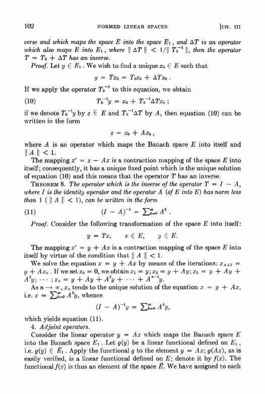
102 NORMED LINEAR SPACES [CH. III
verse and which maps the space E into the space El , and !1T is an operator which also maps E into E l , where II !1T" < 1/11 TO- l II, then the operator T = To + !1T has an inverse.
Proof. Let y E EJ . We wish to find a unique Xo E E such that
!J = Txo = Toxo + !1Txo .
If we apply the operator TO- l to this equation, 've obtain
(10) To-ly = Xo + To-I!1Txo ;
if we denote To-Iy by z E E and To- I!1T by A, then equation (10) can be written in the form
z = Xo + Axo,
where A is an operator which maps the Banach space E into itself and
"A" < 1. The mapping x' = z - Ax is a contraction mapping of the space E into itself; consequently, it has a unique fixed point which is the unique solution of equation (10) and this means that the operator T has an inverse.
THEOREM 8. The operator which is the inverse of the operator T = I - A, where I is the identity operator and the operator A (of E into E) has norm less than 1 ( " A II < 1), can be written in the form
(11)
Proof. Consider the following transformation of the space E into itself:
y = Tx, x E E, y E E.
The mapping x' = y + Ax is a contraction mapping of the space E into itself by virtue of the condition that " A " < 1.
'We solve the equation x = y + Ax by means of the iterations: X n +! =
y + A:rn . If we set Xo = 0, we obtain Xl = y; X2 = Y + Ay; Xa = JJ + Ay + A 2y; ... ;xn =y+Ay+A2y+ '" + An-Iy.
As n ~ oc, Xn tends to the unique solution of the equation :1' = y + Ax, i.e. x = L:'o Aky, whence
(I - A)-Iy = L:'o A ky,
which yields equation (11). 4. Adjoint operators. Consider the linear operator y = Ax which maps the Banach space E
into the Banach space EI .. Let g(y) be a linear functional defined on EI , i.e. g(y) E EI . Apply the functional g to the element y = Ax; g(Ax), as is easily verified, is a linear functional defined on E; denote it by f(x). The functionalf(x) is thus an element of the space E. We have assigned to each

§29] LINEAR OPERATORS 103
functional g E El a functional fEE, i.e. we have obtained an operator which maps El into E. This operator is called the adjoint operator of the operator A and is denoted by A * or by f = A *g.
If we use the notation (f, x) for the functional f(x) , we obtain (g, Ax) = (f, :r), or (g, Ax) = (A *g, x). This relation can be taken for the definition of the adjoint operator.
EXAMPLE. The expression for the adjoint operator in finite-dimensional space. Euclidean n-space En is mapped by the operator A. into Euclidean m-space Em. The operator A is given by the matrix (aij).
The mapping y = Ax can be written in the form of the system
The operator f(x) can be written in the form
f(x) = 2:i=1 fjxj .
The equalities
i = 1,2, ... ,m.
f(x) = g(Ax) = 2:'::"1 giYi = 2:7-1 2:;-1 giaijXj = 2:;:"1 l·j 2:7:'1 gia;,
imply that fj = 2:;=1 giaij . Since f = A *g, it follows that the 'operator A * is given by the transpose of the matrix for the operator A.
We shall now list the basic properties of adjoint operators. 1. The adjoint operator of the sum of two linear operators is equal to th('
sum of the adjoint operators:
(A + B)* = A * + B*.
Letfr = A*g,f2 = B*g,orfl(x) = g(Ax),/2{x) = g(Bx); then (/1 + /2) (x) = g(Ax + Bx) = g[(A + B)x], whence (A + B)* = A* + B*.
2. The adjoint operator of the operator kA, where k is a scalar multiplier, is equal to the adjoint operator of A, mUltiplied by k:
(kA)* = kA*.
The verification of this property is elementary and is left to the reader. :1. J* = J, i.e. the adjoint of the identity operator on E is the identity
operator on E. THEOREM 9. The operator A-*, the adjoint of a linear operator A which
maps the Banach space E into the Banach space E 1 , is also linear and II A* II = IIA II·
Proof. The linearity of the operator A * is obvious. We shall prove the equality of the norms. By virtue of the properties of the norm' of a,n operator we ha,'e:
I f(x) I = I g(Ax) i ::; II g 1111 ..1.1: II ::; II g 1111 A 1111 :r II,

104 NORMED LINEAR SPACES [CR. III
whence II f II :::; II A II II g II or II A *g II :::; II A II II g II and consequently,
(12) II A * II :::; II A II·
Let x E E and form yo = Ax/II Ax II E El ; it is clear that II Yo II = 1. From the corollary to the Hahn-Banach theorem, there exists a functional g such that II g II = 1 and g(yo) = 1, i.e. g(Ax) = II Ax II.
From the inequalities II Ax !I = I (g, Ax) I = I (A *g, x) I :::; II A *g 1111 x II :::; II A * II II g II II x II = il A * II II x II we obtain II A II :::; II A * II which, combined with inequality (12), yields II A II = II A * II.

ADDENDUM TO CHAPTER ITI
Generalized Functions
In 3. number of cases in analysis and in its various applications, for example in theoretical physics, the need arises to introduce various "generalized" functions in addition to the "ordinary" functions. A typical example of this is the well-known t5-function which we have already mentioned above (§23, Example 4).
'Ne wish to emphasize, however, that these concepts, which are discussed briefly in this addendum, did not in any sense originate in an attempt to generalize the concepts of analysis merely for the sake of generalizing. Rather, they were suggested by perfectly concrete problems. Moreover, essentially t.he same concepts were used by physicist.s for quite Home time before they attracted t.he attent.ion of mathemat.icians.
The method of int.roducing generalized functions which we shall use below originat.ed in the work of S. L. Sobolev, published in 1935-36. Later, these ideas were .developed in a somewhat. extended form by L. Schwartz.
Consider on the real line the set D of funct.ions 'P(x) each of which vanishes out.side some interval (where for each 'P there is a corresponding int.erval) and has derivat.ives of all orders. The elements of D can be added and mult.iplied by a scalar in t.he usual way. Thus, D is a linear space. We shall not. int.roduce a norm int.o this space; however, in D one can define in a natural way t.he convergence of a sequence of elements. We shall say that 'Pn ~ 'P if: 1) there exists an interval in the exterior of which all 'Pn and 'P are equal to zero and 2) the sequence of derivatives 'Pn (k) of order k (k = 0,1, 2, ... ) (where t.he derivat.ive of order zero is understood to be as usual the function it.self) converges uniformly t.o 'P(k) on t.his interval. The fact t.hat this concept. of convergence is not. connect.ed with any nonn does not give rise to any inconveniences.
We now introduce the concept. of generalized function. DEFINITION 1. A generalized function (with values on the real line
- 'X) < t < 'Xl) is any linear funct.ional 1'('P) defined on the space D. Thus, 1'('P) sat.isfies t.he following condit.ions:
1. 1'(0l'P1 + (3f1'2) = Ol1'('Pl) + (31'('P2); 2. If 'P,. ~ 'P (in the sense indicat.ed above), then T('Pn) ~ T('P). 'Ve now consider several examples. 1. Let. f(t) be an arbitrary cont.inuous funct.ion of t. Then, since every
function 'P(t) E D vanishes outside some finite interval, the int.egral
(1)
exist.s for all 'P E D. The expression (1) represents a linear funct.ional on
105

106 ADDENDUM TO CHAP,]'I-:R III [CH. III
D (it is left to the reader to verify that Conditions 1 and 2 of Definition 1 are actually fulfilled), i.e. (1) represents a generalized function. Thus, every "ordinary" continuous function is at the same time a generalized function also.
In this connection, two distinct continuous functions will define distinct functionals on D, i.e. they will represent distinct generalized functions. Obviously, it is sufficient to show that every continuous function J(t) which is not identically zero defines a linear functional which is not equal to zero, i.e. to show that there is a function fI'(t) E D for which
L: J(t)fI'(t) dt ~ O.
Since J(t) ¢ 0, an interval (a, fJ) can be found on which J(t) is different from zero and consequently keeps the same sign (for instance, positive). Let us consider the function
This function is positive on the interval (a, fJ); it assumes the value zero at t = a, fJ and this is true of its derivatives of all orders. Consequently, the function fI'(a,/n(t) which is equal to e-1 /(t-a)2 'e-1/(t-P)2 on the interval (a, fJ) and is zero outside this interval, has continuous derivativeH of all orders, i.e. it belongs to D. Furthermore,
L: J(t)fI'(a,p)(t) dt = £P J(t)fI'(a,p)(t) dt > 0,
since the function under the integral sign is positive. 2. We now set
(2) T(fI') = fI'(O).
Formula (2) defines a linear functional on D, i.e. a generalized function. This is none other than the t5-function which we have already mentioned above. (In §23 we considered the l5-function as a functional defined on the space of all continuous functions. The advantages of the point of view adopted here will be manifest in the sequel.)
3. Set T(fI') = -fI"(O).
This generalized function is called the derivative of the t5-function and is denoted by 15'. (A more general definition of the derivative of a generalized function will be given below.)
It is sometimes convenient to denote the generalized function, as in the case of an ordinary function, by the symbol J(t) and say that the linear functional T is "defined" by oome generalized function J(t). The value T(fI') of a linear functional T for each function fI' E D in this context. is more
ADDENDUM GENERALIZED FUNCTIONS 107
conveniently written in the form of a "scalar product" (j, q». If f(t) is a "proper" function,
(f, q» = L: !(t)q>(t) dt.
Frequently, especially in physics books, such an integral notation is used also for generalized functions, for example, we find:
L: t5(t)q>(t) dt = q>(O);
however, it is necessary to remember here that such an integral is only a symbolic representation of the value of the corresponding functional and that it has no other meaning.
We shall now introduce the concept of the limit of a sequence of generallized functions.
DEFINITION 2. The sequence {Tn I is said to converge to the generalized function T if Tn(q» ~ T(q» uniformly on every "bounded" set in D. In this connection, the set {q>l cD is said to be bounded if: 1) there exists a finite interval outside of which all the q> of this set equal zero and 2) it is possible to choose constants Mo , Ml ,M2 , ••• such that
Ill' I < Mo ; Ill" I < lV[l ; Ill''' I < M2 ; ...
for allq> E {q> I. It is easily verified that in the sense of this definition the t5-function is the
limit, for example, of such a sequence of "proper" functions:
lnl 2 for -lin < t < lin, !n(t) =
o for all other values of t.
In exactly the same way it is easy to construct a sequence of "proper" functions converging in the indicated sense to the generalized function 15'. In general, it can be proved that every generalized function is the limit of some sequence of linear functionals defined by "proper" functions.
We shall now formulate the definition of the derivative of a generalized function.
We consider first of all the linear functional T defined by means of a differentiable function:
T(q» = L: !(t)q>(t) dt.
It is natural to call the functional defined by means of the formula
T'(q» = ~~ (q» = L: !'(t)q>(t) dt
the derivative T' of T.

108 ADDENDUM TO CHAPTER III [CH. III
Making use of the formula for integration by parts and taking into consideration the fact that every function q;(t) is differentiable and equal to zero in the exterior of some finite interval, we can rewrite the last expression in the form
T' (q;) = - L: f(t)q;' (t) dt
in which the derivativef'(t) is no longer present in any way. This discussion brings us to the following definition. DEFINITION 3. Let T be a generalized function. Its derivative T' is a
functional defined by the formula
T'(q;) = - T(q;').
It is clear that T' has meaning for all q; E D and represents a generalized function.
Derivatives of the second, third and higher orders are defined analogously.
The validity of the following assertions follows directly from the definition.
THEOREM 1. Every generalized function has derivatives of all orders. THEOREM 2. If the sequence {T,,} converges to the generalized function T
(in the sense of Definition 2), then the sequence of derivatives {T ,,'} converges to T'. In other words: every convergent series of generalized functions can be differentiated term by term any number of times.
It is now clear that the functional ~' (see Example 3) which we called the derivative of the ~-function is in reality the derivative of ~(t) in the sense of Definition 3.
REMARK. The concept of the derivative of a generalized function can be introduced in a somewhat different way. Namely, we define the translation T" of the functional T (where h is an arbitrary number) by setting
T,,(q;(t)) = T(q;(t - h))
(for example, ~,,(q;) = q;( -h), ~,,'(q;) = -q;'(-h), and so forth). Then it is not difficult to verify that the limit
lim1&-.o [(T" - T)/h]
exists and is equal to the derivative T' of the functional T. 4. If the functional T(q;) is defined by means of a differentiable function
f(t), then the functional T' is defined by the functionf'(t), i.e. the generalized derivative of a function coincides with its ordinary derivative if the latter exists.
5. Let T be defined by the function

ADDENDUM
Then
and
i.e. T' is the c5-function.
GENERALIZED FUNCTIONS
11 for t ~ 0, f(t) =
o for t < O.
109
6. If f(t) is a piecewise continuous function having a derivative at all points of continuity, its generalized derivative at points of continuity coincides with its ordinary derivative and at each point of discontinuity t = to it is equal to the c5-function c5(t - to) multiplied by the magnitude of the jump of the function at this point.
7. If
(3) f(t) = L:'::=1 (sin nt)/n,
then the generalized derivative of f(t) equals
L:'::=1 cos nt = - t + 11" L:~--oo c5(t - 2k1l").
We emphasize that the series on the left in the last equation converges in the sense of convergence for generalized functions (Definition 2). Series (3) can be differentiated term by term any number of times.
The last example shows that the concept of generalized function allows us to assign a perfectly definite meaning to the sum of a series which diverges in the ordinary sense. The same remark applies also to many divergent integrals. This situation is frequently encountered in theoretical physics where in each individual case special methods are used to give a definite meaning to a divergent series or to a divergent integral.
In an analogous way, we can introduce generalized functions of several independent variables. To do this, it is merely necessary to take as the initial space D the space of all functions of n variables which are differentiable an infinite number of times and each of which vanishes outside some sphere. All the concepts introduced above carryover automatically to this case. It is easy to verify that every generalized function of several independent variables has partial derivatives of all orders and that the result of differentiating with respect to several variables does not depend on the order of differentiation.

Chapter IV
LINEAR OPERATOR EQUATIONS
§30. Spectrum of an operator. Resolvents
Throughout this entire chapter we shall consider bounded linear operators which map a (generally speaking complex) Banach space E into itself. An operator adjoint to an operator of the type indicated will, obviously, map the conjugate space E into itself.
In the study of linear operators in finite-dimensional space an important role is played by the concepts of characteristic vector and characteristic value. In the case of n-dimensional space the concept of the characteristic value of an operator can be introduced by means of the following equivalent methods:
1) The number A is said to be a characteristic value of the operator A if there exists a nonzero vector x (characteristic vector) such that Ax = AX.
2) The number A is said to be a characteristic value of the operator A if it is a root of the characteristic equation
Det I A - AI I = o. The first of these definitions carries over without any changes to the
case of infinite-dimensional space, i.e. it can be considered as the definition of characteristic values of an operator in infinite-dimensional space.
The second of the definitions formulated above does not carryover directly to the infinite-dimensional case since the concept of determinant does not have meaning in infinite-dimensional space. However, this second definition can be changed in form in the following manner. The fact that the determinant of the matrix A - AI is zero is equivalent to the fact that this matrix has no inverse, i.e. we can say that the characteristic values A are those numbers for which the inverse of the operator A - AI does not exist. Taking this as our point of departure we introduce the following definition.
The totality of those values A for which the inverse of the operator A - AI does not exist is called the spectrum of the operator A. The values of A for which the operator A - AI has an inverse are said to be regular; thus, the spectrum consists of all nonregular points. In this connection, the operator R-,.. = (A - AI)-l itself is called the resolvent of the operator A. In n-dimensional space the concepts of characteristic value and nonregular, or singular, point coincide. In the general case, as the example to be introduced below will show, this is no longer the situation. The spectrum necessarily contains all the characteristic values but it may contain, besides these, other num-
110

§30] SPECTRUM OF AN OPERATOR. RESOLVENTS 111
bers also. The set of characteristic values is called the point spectrum of the operator A. The remaining part of the spectrum is called the continuous spectrum. (This is not the usual terminology. The remaining part of the spectrum consists of two parts: 1) Those values of X for which A - >..I has an unbounded inverse with domain dense in E form the continuous spectrum. 2) The remainder of the spectrum, consisting of those values of X for which A - >..I has an inverse whose domain is not dense in E, is called the residual spectrum.-Trans.)
If the point X is regular, i.e. if the inverse of the operator A - >..I exists, then for sufficiently small ~ the operator A - (X + ~)I also has an inverse (Theorem 7, §29), i.e. the point X + ~ is regular also. Thus, the regular points form an open set. Consequently the spectrum, which is its complement, is a closed set.
THEOREM 1. 'l'he inverse of the operator A - >..I exists for arbitrary X for which I X I > II A II·
Proof. Since we obviously have
i1 - >..I = - X (I - ~ A ),
then
R" = (A - XI)-I = -(1/X) (I - A/2)-1 = -(I/X) L~o Ak/Xk.
This series converges for II A/X II < 1 (see Theorem 8, §29), i.e. the operator A - >..I has an inverse. In other words, the spectrum of the operator A is contained in a circle of radius II A II with center at zero.
EXAMPLE. Let us consider in the space C the operator A defined by the formula
A (x(t)) = p.(t)x(t),
where p.(t) is a fixed continuous function. We have
(A - Xl)x(t) = (p.(t) - X)x(t),
whence
(A - XI)-lx(t) = /1/[p.(t) - X]}x(t).
The spectrum of the operator A under consideration consists of all X for which p.(t) - X is zero for some t lying between 0 and 1, i.e. the spectrum is the totality of all values of the function p.(t). For example, if p.(t) = t, then the spectrum is the closed interval [0, 1]; in this case characteristic values a.re absent, i.e. the operator defined as multiplication by t is an example of an operator with a purely continuous spectrum.
(1) Every linear operator, defined in a Banach space which has at least
112 LINEAR OPERATOR EQUATIONS [CR. IV
one nonzero element, has a nonvoid spectrum. Operators exist for which the spectrum consists of a single point (for example, the operator defined as multiplication by a scalar).
(2) Theorem 1 can be sharpened in the following way. Let r = inf II An IIl/n; then the spectrum of the operator A lies entirely in a circle with radius r and center at zero.
(3) The resolvent operators R,. and Rx corresponding to the points p.
and X are commutative and satisfy the relation
R,. - Rx = (p. - X)R,.Rx
which is easily verified by multiplying both sides of this equality by (A - XI) (A - p.J). From this it follows that the derivative of Rx with respect to X, i.e.
liml1x ... o (Rx+l1x - Rx)/I1X,
exists and is equal to Rx2•
§31. Completely continuous operators
DEFINITION. An operator A which maps a Banach space E into itself is said to be completely continuous if it maps an arbitrary bounded set into a compact set.
In finite-dimensional space every bounded linear operator is completely continuous since it maps an arbitrary bounded set into a bounded set and in finite-dimensional space every bounded set is compact.
But in the case of infin!te-dimensional space there always exist operators which are bounded (i.e. continuous) but which are not completely continuous; such, for example, is the identity operator in infinite-dimensional space.
An extensive class of completely continuous operators y = Ax in the space C[a, b] can be written in the form
(1) y(s) = { K(s, t)x(t) dt.
THEOREM 1. Formula (1) defines a completely continuous operator in the space C[a, b] if the function K(s, t) is bounded on the square a :::; s :::; b, a :::; t :::; b and all points of discontinuity of the function K (s, t) lie on a finite number of curves
k = 1,2 .... ,n, where the f{Jk are continuous functions.
REMARK. The distribution of points of discontinuity on the straight lines s = constant is essential here. For example, for a = 0, b = 1, the

§31)
kernel
COMPLETELY CONTINUOUS OPERATORS
(1 for s < !, K(s, t) = 1
lO for s ~ !
113
has for points of discontinuity all the points of the square with s = !. In this case transformation (1) maps the function x(t) = 1 into a discontinuous function.
Proof of Theorem 1. We note that under the conditions of the theorem, integral (1) exists for arbitrary s in the closed interval a ~ s ~ b. Let M =
sup I K(s, t) I on the square a ~ s ~ b, a ~ t ~ b. Denote 'by G the set of points (s, t) for which I t - ~k(S) I < ~/12Mn holds for arbitrary k =
1,2, ... , n; denote by F the complement of G with respect to the square a ~ s ~ b, a ~ t ~ b. Since F is closed and K(s, t) is continuous on F, there exists a 0 such that for points (s', t), (s", t) in F for which I s' .- s" I < 0 the inequality
I K(s', t) - K(s", t) I < ~/3(b - a)
holds. Now let s' and s" be such that Is' - s" I < o. Then
I y(s') - y(s") I ~ t I K(s', t) - K(s", t) II x(t) I dt ·a
can be evaluated by integrating over the sum of the intervals
I t - ~k(S') I < ~/12Mn, I t - ~k(S") I < ~/12Mn
(denote this sum by A) and over the complement B of A with respect to the closed interval [a, b]. The length of A does not exceed ~/3M. Therefore
L I K(s', t) - K(s", t) II x(t) I dt ~ (2~/3) II x II .
The integral over B, obviously, may be estimated by
fa I K(s', t) - K(s", t) II x(t) I dt ~ (~/3) II x II .
Therefore,
I y(s') - y(s") I ~ ~ II x II·
We have proved the continuity of y(s) and the equicontinuity of the functions y(s) corresponding to the functions x(t) with bounded norm. The uniform boundedness of y(s) corresponding to the xU) with bounded norm

114 LINEAR OPERATOR EQUATIONS [CH. IV
follows from the inequalities
I y(S) I :::; t I K(s, t) I I X(t) I dt :::; M(b - a) II x Ii .
The Volterra Operator. If we assume that K(s, t) = 0 for t > s, then the operator (1) takes on the form
(2) y(s) = { K(s, t)x(t) dt.
We shall assume the function K(s, t) to be continuous for t :::; s. The validity of the hypothesis of Theorem 1 is easily verified for such a kernel. Consequently this operator is completely continuous.
We shall now establish several properties of completely continuous operators.
THEOREM 2. If {An} is a sequence of completely continuous operators on a Banach space E which converges in norm to an operator A, then the operator A is completely continuous.
Proof. Let us consider an arbitrary bounded sequence of elements in E: Xl , X2, ... ,Xn , . .. ; II Xn II < c. It is necessary to prove that the sequence {Axn } contains a convergent subsequence.
The operator Al is completely continuous and therefore we can select a convergent subsequence from the sequence {A IXn}. Let
(3) X (1) n ,
be the inverse images of the members of this convergent subsequence. We apply the operator A2 to each member of the subsequence (3). Since A2 is completely continuous, we can again select such a convergent subsequence from the sequence {A2Xn (1)}, the inverse images of whose terms are, say,
Xl(2), X2(2), ... ,Xn(2\ .,.
We apply the operator A3 to this sequence {Xn (2)} and then in an analo-gous manner select a subsequence Xl (3), X2 (3), Xn (3), •.• , and so on.
We now form the diagonal sequence (1) (2) (n)
Xl ,X2 ,'" Xn
Each of the operators AI, A2, ... , An, ... transforms this sequence into a convergent sequence. If we show that the operator A also transforms this sequence into a convergent sequence, then this will also establish the complete continuity of the operator A. Let us evaluate the norm of the difference AXn (n) - A_xm (m):
II AXn (n) - AXm (m) II :::; II AXn (n) - Akxn (n) II + II Akxn(n) - Akxm(>n) II + II Akxm(m) - Axm(m) II
:::; II A - Ak II (II Xn (n) II + II Xm (m) II) + II Akxn (n) - Akxm (m) II.

§31] COMPLETELY CONTINUOUS OPERATORS 115
We choose k so that II A - Ak II < E/(2c) and N such that the relation
II A~.xn (n) - AkXm (m) II < E/2
holds for arbitrary n > Nand m > N. (This is possible because the sequence IAkxn(n)} converges.) Then II Axn(n) - Axm(m) II < E, i.e. the sequence II AXn (n) II is fundamental.
Since the space E is complete, this sequence converges; this proves the theorem.
THEOREM 3. The adjoint operator of a completely continuous operator is completely continuous.
Proof. Let the operator A map the Banach space E into itself. Then the operator A *, adj oint to A, maps the space E into itself. Inasmuch as an arbitrary bounded set can be enclosed in a sphere, the theorem will be proved if we prove that the image of the sphere S belonging to the space E (i.e. the set A * S) is compact. It is obviously sufficient to carry out the proof for the case of the unit sphere.
We introduce into the space E the auxiliary metric obtained by setting for any two functionals g', gil in E,
(4) p(g', gil) = sup II g'(y) - g"(y) I; yEAS}.
Since the operator A is completely continuous by hypothesis, the image AS of the unit sphere S is compact in the space E. If YEAS, then II y II ::;; II A II. Consequently if g E S, then I g(y) I ::;; II g 1111 y II ::;; II A II, i.e. the functionals g(y) E S are uniformly bounded in the sense of metric (4).
Further, we have
I g(y') - g(y") I ::;; II g II II y' - y" II ::;; II y' - y" II,
i.e. the functionals g(y) E S are equicontinuous. In accordance with Arzela's theorem, §17, this means that the set S is compact in the sense of metric (4). But since
II A *g' - A *g" II ::;; sup II g'(Ax) - g"(Ax) I; xES},
the compactness of the set S in the sense of metric (4) implies the compactness of the set A * S in the sense of the original metric of the space E.
THEOREM 4. If A is a completely continuous operator and B is a bounded operator, then the operators AB and BA are also completely continuous.
Proof. If M is a bounded set in E, then the set BM is also bounded. Consequently, the set ABM is compact and this means that the operator AB is completely continuous. Further, if M is bounded, then AM is compact; but then in virtue of the continuity of B, the set BAM is also compact. This completes the proof of the theorem.
COROLLARY. A completely continuous operator A cannot have a bounded inverse in an infinite-dimensional space E.

116 LINEAR OPERATOR EQUATIONS [CR. IV
In fact, in the contrary case the identity operator I = AA -1 would be completely continuous in E, which is impossible.
We shall now study the spectrum of a completely continuous operator. THEoREM 5. Every completely continuous operator A in the Banach space E
has for arbitrary p > 0 only a finite number of linearly independent characteristic vectors which correspond to the characteristic values whose absolute values are greater than p.
Proof. Let us assume that this is not the situation, i.e. let us assume that there exists an infinite number of linearly independent characteristic vectors x" (n = 1, 2, ... ), satisfying the condition
(5) IX"I > p> 0, (n = 1,2, ... ).
Consider in E the subspace El generated by the vectors x". In this subspace the operator A has a bounded inverse. In fact, vectors of the form
(6)
are everywhere dense in El . For these vectors,
Ax = CX1X1Xl + CX2X2X2 + ... + CXkXkXk
and consequently,
(7) A -IX = (CXl/X1)Xl + (CX2/X2)X2 + ... + (CXk/X,.)X,.
and II A-Ix II ~ (l/p) II x II.
Consequently the operator A -\ defined for vectors of the form (6) by means of formula (7), can be extended by continuity (and consequently with preservation of norm) to all of El . The operator A, being completely continuous in E, is completely continuous in El also. But according to the corollary to the preceding theorem a completely continuous operator cannot have a bounded inverse in infinite-dimensional space. The contradiction thus obtained proves the theorem. It follows from this theorem that every nonzero characteristic value of a completely continuous operator has only finite multiplicity and these characteristic values form a bounded set which cannot have a single limit point distinct from the origin of coordinates. We have thus obtained a characterization of the point spectrum of a completely continuous operator. It will follow from the results of the next section that a completely continuous operator cannot have a continuous spectrum.
§32. Ljnear operator equations. The Fredholm theorems
In this section we shall consider equations of the form
(1) y = x - Ax,

§32] LINEAR OPERATOR EQUATIONS. FREDHOLM'S THEOREMS 117
where A is a completely continuous operator which maps a Banach space E into itself. We shall show that for such equations a number of theorems are valid which are analogous to the known theorems for systems of linear algebraic equations. First of all the corresponding theory was developed by Fredholm for integral equations of the form
(2) ((J(t) = f(t) + { K(s, t)({J(s) ds,
where f(t) and K(s, t) are given continuous functions. It was established in the preceding section that the Fredholm operator
yet) = { K(s, t)x(s) ds
is completely continuous; thus, equation (1) actually is a generalization of the Fredholm integral equation (2).
THEOREM 1. Let A be a completely continuous operator which maps the Banach space E into itself. If the equation y = x - Ax is solvable for arbitrary y, then the equation x - Ax = 0 has no solutions distinct from the zero solution.
Proof. Let us assume the contrary: suppose there exists an element Xl ~ 0 such that Xl - AXI = TXI = o. Those elements X for which Tx = 0 form a linear subspace EI of the space E. Let us denote by En the subspace consisting of the elements which satisfy the condition Tnx = o.
It is clear that the subspaces En form a nondecreasing subsequence
EI ~ E2 C ... C En C ....
We shall show that the equality sign cannot hold at any point of this chain of inclusion relations. In fact, since by assumption Xl ~ 0 and the equation y = Tx is solvable for arbitrary y, we can find a sequence of elements distinct from zero Xl , X2, ... , Xn , ... , such that
TX2 = Xl
TXn = Xn-l
The element Xn belongs to the subspace En for each n but it does not belong to the subspace En_I. In fact,
Tnxn = Tn-Ix,,_l = ... = TXI = 0,
but

118 LINEAR OPERATOR EQUATIONS [CR. IV
All the subspaces En are linear and closed; therefore for arbitrary n there exists an element Yn+l E E n+l such that
II Yn+l II = 1 and P(Yn+l, En) 2: t, where P(Yn+l , En) denotes the distance from Yn+l to the space En , i.e.
P(Yn+l, En) = inf {II Yn+l - X II; X E En}.
[In fact, if we let p(Xn+l , En) = a, then we can find an element x E En such that II Xn+l - X II < 2a; at the same time we clearly have P(Xn+l -x, En) = P(Xn+l, En) = a. We can then set Yn+l = (Xn+l - x)/II Xn+l - X II.] Consider the sequence {Ayk\ . We have (assuming p > q):
II Ayp - AYq II = II yp - (Yq + Typ - TYq) II 2: t, since yq + Typ - Tyq E Ep_l • It is clear from this that the sequence {Ayd cannot contain any convergent subsequence, which contradicts the complete continuity of the operator A. The contradiction thus obtained proves the theorem.
COROLLARY 1. If the equation y = X - Ax is solvable for arbitrary y, then it has a unique solution for each y, i.e. the operator I - A has an inverse in this case.
In fact, if the equation y = x - Ax had two distinct solutions for some y, say Xl and X2 , then the equation x - Ax = 0 would have a nonzero solution Xl - X2, which contradicts Theorem 1.
In the sequel it is convenient to consider together with the equation y = x - Ax the equation h = f - A *f which is adjoint to it, where A * is the adjoint of A and h, f are elements of the Banach space it, the conjugate of E.
For the adjoint equation we can formulate the following result. COROLLARY 2. If the equation h = f - A *f is solvable for all h, then the
equation f - A *f = 0 has only the zero solution. This assertion is obtained from Theorem 1 if we recall that the operator
adjoint to a completely continuous operator is completely continuous (Theorem 2, §31) and a space conjugate to a Banach space is itself a Banach space.
THEOREM 2. A necessary and sufficient condition that the equation y ::; x - Ax be solvable is that the following condition be fulfilled: fey) = 0 for all f for which f - A *f = o.
Proof. 1. If we assume the equation y = x - Ax is solvable, then fey) = f(x) - f(Ax) = f(x) - A *f(x) , i.e. fey) = 0 for all f which satisfy the condition f - A *f = O.
2. Now letf(y) equal zero for allf which satisfy the equationf - A *f = O. For each of these functionals f we shall consider the set L, of elements for

§32] LINEAR OPERATOR EQUATIONS. FREDIIOU\f'S THJ<JOREMS 119
which f takes on the value zero. Then our assertion is equivalent to the fact that the set nLr consist.s only of the element.s of the form x - A:r, i.e. it is necessary for us to prove that an element Yl which cannot be represented in the form x - Ax cannot be contained in nLr . To do this we shall show that for such an element 1/1 we can construct a functional II which satisfies the conditions
II - A*ft = O.
These conditions are equivalent to the following:
fl(X - Ax) = 0 for all x.
In fact,
(fl - A *fl) (x) = ft(x) - A *ft(x) = fl(X) - fl(Ax) = ft(x - Ax).
Let Go be the subspace consisting of all elements of the form x - Ax. Consider the subspace I Go , Yl} , i.e. the set of elements of the form z + aYI , z E Go, and define t.he linear functional fl on this subspace by setting
fl(Z + aYl) = a.
Extending this functional to the whole space E (which is possible by virtue of the Hahn-Banach theorem) we do obtain a linear functional satisfying the required condit.ions. This completes the proof of the theorem.
COROLLARY. If the equation f - A *f = 0 does not have nonzero solutions, then the equation x - Ax = y is solvable for all y.
We shall now establish the analogue of Theorem 2 for the adjoint equation.
THEOREM 3. A necessary and sufficient condition that the equation
(3) h=f-A*f
be solvable is that h(x) = 0 for all x for which x - Ax = O. Proof. 1. If the equation h = f - A ~f is solvable, then
h(x) = f(x) - A *I(x) = f(x - Ax),
i.e. h(x) = 0 if x - Ax = O. 2. Now let h(x) = 0 for all x which satisfy the equation x - Ax = O.
We shall show that equation (3) is solvable. We shall construct the functionalI on the set F of all elements of the form 11 = :l~ - Ax by setting
(4) f(Tx) = h(x).
This equation in fact defines a linear functional. li'irst of all we note that the value of the functional I is defined uniquely for each y because if TXl = TX2, then h(Xl) = h(X2). It is easy to verify the linearity of the func-

120 LINEAR OPERATOR EQUATIOKS [CH. IV
tional (4). This functional can be extended to the whole space E. We obtain
f(Tx) = T*f(x) = h(x),
i.e. this functional is a solution of equation (3). COROLLARY. If the equation x - Ax = 0 has no nonzero solutions, then
the equation f - A *f = h is solvable for all h. The following theorem is the converse of Theorem 1. ThEOREM 4. If the equation x - Ax = 0 has x = 0 for its only solution,
then the equation x - Ax = y has a solution for all y. Proof. If the equation x - Ax = 0 has only one solution, then by virtue
of the corollary to the preceding theorem the equation f - A *f = h is solvable for all h. Then, by Theorem 1, Corollary 2, the equationf - A *f = o has only the zero solution. Hence the Corollary to Theorem 2 implies t.he solvability of the equation y = x - Ax for arbitrary y.
Theorems 1 and 4 show that for the equation
(1) y = x - Ax
only the following two cases are possible: 1) Equation (1) haR a unique solution for each y, i.e. the operator I-A.
has an inverse. 2) The equation x - Ax = 0 has a nonzero solution, i.e. the number
>. = 1 is a characteristic value for the operator A. It is clear that all the results obtained above for the equation y = x - Ax
carryover automatically also to the equation y = x - >.Ax, where>. is an arbitrary number. (For such an equation the adjoint equation will be h = f - XA *f.) It follows that either the operator I - >.A has an inverse or that the number 1/>. is a characteristic value of the operator A. In other words, in the case of a completely continuous operator, an arbitrary number is either a regular point or a characteristic value, i.e. a completely continuous operator has only a point spectrum. The point spectrum of a completely eontinuous operator was studied in the preceding section (Theorem 5).
ThEOREM 5. The dimension n of the space N whose elements are the solutions of the equation x - Aa: = 0 is equal to the dimension of the subspace N* whose elements are the solutions of the equation.f - A *f = O.
Proof. We note first that in virtue of the complete continuity of the operators A and A *, the subspaces Nand N* are finite-dimensional. Let {Xl, X2, •• , , x n } be a basis for the subspace N and let Ifl' f2, ... ,f.} be a basis for the subspace N*. According to the Hahn-Banach theorem on the extension of a linear functional, n funet.ionals ~l , ~2, ••• , ~n can be constructed which satisfy the conditions
11 for i = j, ~j(Xi) =
o for i ~ j.

§32] LINK~R OPERATOR EQUATIONS. I!'REDHOLM'S THEOREMS 121
We now consider the functionals 11 , J2, ... , f. and construet for each of them the corresponding subspace Li , defined by the condition 1;(:1:) = O. Since the functionals Ii are linearly independent, the corresponding :>ets Li are distinct; and since each of the subspaces Li has iudex 1, a relation of the form L j C Li is likewise impossible.
Let us consider the sets
L2 n L3 n ... n L. '" L1 n L2 n ... n L. = ill1 ;zE O.
The set Mi consists of those elements which belong to all L j , except Li . It is clear that the sets Mi are disjoint. Since all the functionals 11 , h, ... , I. , except Ii , assume the value zero on JlI i and since M i is a linear manifold, it is possible to choose a point Zi in each Mi to satisfy the following conditions:
(5) 11 for i = j, I -(Zi) =
1 0 for i ;zE j.
Mter these auxiliary constructions we pa~s directly to the proof of the assertion of the theorem.
We assume first that P > n. We construct the operator
R(x) = Ax + L:;:"1 fPj(x)Zj .
This operator is completely continuous since it is the sum of a finite number of completely continuous operators. Further, let us consider the operator
W(x) = x - R(x) = ;r - A:t~ - L:i =1 fPj(X)Zj .
We shall show that if W(xo) = 0, then Xo = O. Let us apply the functional Ii to W(xo):
(6) j;(W(xo)) = li(TxO) - L:;:"1 fPj(XO)li(Zj) = li(TxO) - fPi(XO).
Since, by hypothesis, Ii satisfies the equation T*li = O,li(Tx) = 0 for all x (i = 1,2, ... , p). Besides,li(W(xo)) = 0 since, by assumption, TVxo = O. Therefore from (6) it follows that
(7) li = 1, 2, ... , It).
But then the equation Wxo = 0 implies that Txo = 0, i.e. :ro E N; since the elements Xl , X2, ••• , Xn form a basis in N, we have
:l~o = 0!1X1 + 0!2X2 + ... + O!nXn •

122 LINEAR OPERATOR EQUATIONS [CH. IV
If we apply the functional Vii to this equation and make use of equations (7), we see that (Xi = Vii (XO) • This and (7) imply that Xo = O. We have shown that the equation Wx = 0 has only the zero solution. From this it follows (Theorem 4) that the equation Wx = y is solvable for all y and, in particular, for y = Zn+l .
Let x be a solution of the equation W x = Zn+l. Then, on the one hand, it follows from the fact that T*fn+l = 0 and from (5) that
fn+l(Wx) = fn+l(Tx) - fn+l[Li-l Vli(X)Zi] = OJ
on the other hand, according to (5), that
f n+l (Zn+l) = 1.
The contradiction thus obtained proves that 11 ::; n. Let us now assume that n > 11. We construct the operator W* by setting
(8) W*f = T*f - L~=l f(Zi)Vli .
We shall prove that if W*f = 0, thenf = o. We have
(T*f)Xi = 0 (i = 1, 2, ... , n)
for all f since Xi E N. Therefore, if W*f = 0, applying both sides of (8) to Xi , we obtain:
(9) Lk=t!(Zk)Vlk(Xi) = f(Zi) = 0 (i = 1,2, ... , 11).
Thus, the equation W*f = 0 reduces to T*f = 0, i.e. f E N*. Consequently, f can be written in the form
f = flt/l + 1M2 + ... + fli .. If we apply both sides of this equation to the element Zi we see that
fli = f(Zi). From this and (9) it follows that f = O. This implies that the equation W*f = g is solvable for all g.
Let f be such that W*f = VI.+1 . Then, on the one hand,
(W*f) (X.+l) = (T*f) (X.+l) - L~=l f(Zi)VI.(X.+l) = 0,
and on the other,
VI.+1 (X.+l) = 1.
We have thus arrived at a contradiction, which proves that n ::; 11. So finally, n = 11. This completes the proof of the theorem.
LIST OF SYMBOLS Page Page
E ................................. 1 EE ................................. 1
C[a, b). .......................... 17 CZ[a, b) ........................... 19

SYMBOLS. DEFINITIONS. THEOREMS
s:: ........................... . (J •......................•........• u ... . n .............................. . A""-B .. . AAB .... . ~o .. c ............... . m ............... . p(x, y) .............. .
R = (X, p). . ........ . R ...... .............. .
Page 1 1 1 2 2 :3
10 10 10 16 16 17
Ro"............. .......... 17 Rp...... ..................... 20 C................................. 18
Page S(Xo ,r) .. , ..................... " 23 S[Xo, rJ ........... , .. .... .. .. . .. . 23 O(x, E)...... . ... . .. . .. .... . . .. .. 23 [MJ..... ........................... 2:J J~~......... . .......... M [(xo). .... . ........... 64 II X II ......... · ....... ·........... 71 ~ ............................... . ~ ............................... .
c ........... , .................... . m .......... ................. . II X lip .... · R ........... ................ . R... ............ .. ...... . T-1 ........... . ........... .
A* .............. .
18 22 72 72 74 82 88 99
103
LIST OF DEFINITIONS Page
Equivalence of sets. . . . . . . . . . . . . . . . . . . . . . . . . . . . . . . . . . . . . . . . . . . . . . . . . . . . . . . . . 7 Metric space. . . . . . . . . . . . . . . . . . . . . . . . . . . . . . . . . . . . . . . . . . . . . . . . . . . . . . . . . . . 16 Complete space. . . . . . . . . . . . . . . . . . . . . . . . . . . . . . . . . . . . . . . . . . . . . . . . . . . . . . . . . . 37 Completion of a space. . . . . . . . . . . . . . . . . . . . . . . . . . . . . . . . . . . . . . . . . . . . . . . . . . . . . . . 39 Linear space. . . . . . . .,. . . . . . . . . . . . . . . . . . . . . . . . . . . . . . . . . . . . . . . . . . . . .. . . . . . 71 Linear manifold.. . . " . . . . . . . . . . . . . . . . . . . . . . . . . . . . . . . . . . . . . . . . . . . . . . . . . . . . 73 Subspace ..... , . . . . . . . . . ................ . . . . . . . . . . . . . . . . . . . . . . . . . . . . . . . . . . . . . 73 Convex set and convex body. . . .. . . . . . . . . . . . . . . . . . . . . . . . . . . . . . . . . . . . . . . . . . . . . 74 Functional and linear functional. . . . . . . . . . . . . . . . . . . . . . . . . . . . . . . . . . . . . . . . . . . . . 77 Norm of a linear functional. . . . . . . . . . . . . . . . . . . . . . . . . . . . . . . . . . . . . . . . . . . . . . . . . 78 Index of a subspace of a Banach space. .. . . . . . . . . . . . . . . . . . . . . . . . . . . . . . . . . . . . . 80 Weakly convergent sequence of elements ........... " . . . .. .. ... .. ............. 90 Weakly convergent sequence of linear functionals .. . . . . . . . . . . . . . . . . . . . . . . . . . . 93 Linear operator.. . . . . . . . . . . . . . . . . . . . . . . . . . . . . . . . . . . . . . . . . . . . . . . . . . . . . . . . . . . . . 95 Bounded operator.. . . . . . . . . . . . . . . . . . . . . . . . . . . . . . . . . . . . . . . . . . . . . . . . . . . . . . . . . . . 95 Continuous operator.. . . . . . . . . . . . . . . . . . . . . . . . . . . . . . . . . . . . . . . . . . . . . . . . . . . . . . . . 95 Norm of a bounded linear operator.. . . . . . . . . . . . . . . . . . . . . . . . . . . . . . . . . . . . . . . . . . 97 Sum of continuous linear operators.. . . . . . . . . . . . . . . . . . . . . . . . . . . . . . . . . . . . . . . . . . 97 Product of continuous linear operators. . . . . . . . . . . . . . . . . . . . . . . . . . . . . . . . . . . . . . . 98 Inverse of an operator. . . . . . . . . . . . . . . . . . . . . . . . . . . . . . . . . . . . . . . . . . . . . . . . . . . . . .. 98 Generalized function ......................................................... 105 Convergence of a sequence of generalized functions .................... '" ... , 107 Derivative of a generalized function .......................................... 108 Completely continuous operator .............................................. 112
LIST OF THEOREMS CHAPTER I
§2 Theorem 10. . ........................................................... . §2 Theorem 20 ••.••.•.•••••••••••••••••••.••.•.•••••••••••••••••••••••••••••
Page
5 5

124 'fHEOREMS
Page §2 'l'heorem 3° . . . . . . . . . . . . . . . . . . . . . . . . . . . . . . . . . . . . . . . . . . . . . . . . . . . . . . . . . 6 §4 Theorem (N ondenumerability of the set of real numbers). . . . .. ............. 8 §5 Theorem (Cnrrliunlit~· of the Ret of all subsets of II lie!) . .. ............. 10 §7 Theorem 1.. . . . . . . . . . . . . . . . . . . . . . . . . . . . . . . . . . . . . . . . . . . . . . . . . . . . . . . . . . . . . .. 14 §7 Theorem 2. . . . . . . . . . . . . . . . . . . . . . . . . . . . . . . . . . . . . . . . . . . . . . . . . . . . . . . . . . . . . . .. 14 §7 Theorem 3. . . . . . .. . . . . . . . . . .. . . . . . . . . . .. . . . . . . . . . . . . . . . . . . .. . . . . . . ... . . . .. 14
CIl,~PTER H
§9 Theorem 1.. . . . . . . . . . . . . . . . . . . . . . . . . . . . . . . . . . . . . . . . . . . . . . . . . . . . . . . . . . . . . . .. 23 §9 Theorem 2. . . . . . . . . . . . . . . . . . . . . . . . . . . . . . . . . . . . . . . . . . . . . . . . . . . . . . . . . . . . . . .. 23 §\J Theorem 3. . . . . . . . . . . . . . . . . . . . . . . . . . . . . . . . . . . . . . . . . . . . . . . . . . . . . . . . . . . . . . .. 23 §9 Theorem 4. . . . . . . . . . . . . . . . . . . . . . . . . . . . . . . . . . . . . . . . . . . . . . . . . . . . . . . . . . . . . . .. 24 §9 Theorem 5. . . . . . . . . . . . . . . . . . . . . . . . . . . . . . . . . . . . . . . . . . . . . . . . . . . . . . . . . . . . . . .. 25 §10 Theorem 1. . . . . . . . . . . . . . . . . . . . . . . . . . . . . . . . . . . . . . . . . . . . . . . . . . . . . . . . . . . . . .. 27 §10 Theorem 2. . . . . . . . . . . . . . . . . . . . . . . . . . . . . . . . . . . . . . . . . . . . . . . . . . . . . . . . . . . . . .. 27 §10 Theorem l' .... . .. . .. .. .. .. .. .. . . . .. . . . . . . . .. .. .. . . .. . ... . . . . .. .. ... . .. ... 28 §10 Theorem 3. . . . . . . . . . . . . . . . . . . . . . . . . . . . . . . . . . . . . . . . . . . . . . . . . . . . . . . . . . . . . .. 28 §10 Theorem 4 ............................................................... 28 §1O TheOI·em 5. . . . . . . . . . . . . . . . . . . . . . . . . . . . . . . . . . . . . . . . . . . . . . . . . . . . . . . . . . . . . .. 29 §1l Theorem 1. . . . . . . . . . . . . . . . . . . . . . . . . . . . . . . . . . . . . . . . . . . . . . . . . . . . . . . . . . . . . .. 31 §12 Theorem 1. . . . . . . . . . . . . . . . . . . . . . . . . . . . . . . . . . . . . . . . . . . . . . . . . . . . . . . . . . . . . .. 34 §12 Theorem 2. . . . . . . . . . . . . . . . . . . . . . . . . . . . . . . . . . . . . . . . . . . . . . . . . . . . . . . . . . . . . .. 34 §12 Theorem 3 . . . . . . . . . . . . . . . . . . . . . . . . . . . . . . . . . . . . . . . . . . . . . . . . . . . . . . . . . . . . . .. 35 §13 Theorem 1. . . . . . . . . . . . . . . . . . . . . . . . . . . . . . . . . . . . . . . . . . . . . . . . . . . . . . . . . . . . . .. 39 §13 Theorem 2. . . . . . . . . . . . . . . . . . . . . . . . . . . . . . . . . . . . . . . . . . . . . . . . . . . . . . . . . . . . . .. 40 §14 Theorem (Prilleiple of contraction mappings) . . . . . . . . . . . . . . . . . . . . . . .. . . . .. 43 §16 Theorem 1. . . . . . . . . . . . . . . . . . . . . . . . . . . . . . . . . . . . . . . . . . . . . . . . . . . . . . . . . . . . . .. 52 §16 Theorem 2. . . . . . . . . . . . . . . . . . . . . . . . . . . . . . . . . . . . . . . . . . . . . . . . . . . . . . . . . . .. . .. 53 §17 Theorem 1 (Arzela)...................................................... 54 §17 Theorem 2 (Peano).. . . . .. . . . . . . . . . . . . . . . . . . . . . . . . . . . . . . . . . . . . . .. .. . . .. .. . 56 §18 Theorem 1. . . . . . . . . . . . . . . . . . . . . . . . . . . . . . . . . . . . . . . . . . . . . . . . . . . . . . . . . . . . . . . 58 §18 Theorem 2. . . . . . . . . . . . . . . . . . . . . . . . . . . . . . . . . . . . . . . . . . . . . . . . . . . . . . . . . . . . . . . 58 §18 Theorem 3.. .. . . . . ... .. .. .. .. .. .. .. . . . . . .. . ... .. .. .. .. .. .. .. . .... ... ..... l.i8 §18 Theorem 4. . . . . . . .. . . . .. .. . ...... .. . . . . . . . .. . . . .. .. . ...... .. . ....... .. ... 58 §18 Theorem 5. . .. . . . . . . ... .. . . . . .. .. .. . . .. . . . . . . ... .. . . . . .. .. .. .. .. . ........ 59 §18 Theorem 6. . . . . . . .. . . .. ....... ... . .. . . . . . . .. . . .. ....... ... . .............. 60 §18 Theorem 7. . . ... . . . .. ... . .... .... .. . . . ... . . . .. ... . .... .... .. . ............ 61 §19 Theorem 1. . . . . . . . . . . . . . . . . . . . . . . . . . . . . . . . . . . . . . . . . . . . . . . . . . . . . . . . . . . . . .. 63 §19 Theorem 2. . . . . . . . . . . . . . . . . . . . . . . . . . . . . . . . . . . . . . . . . . . . . . . . . . . . . . . . . . . . . .. 63 §19 Theorem 3. . . . . . . .. . . . .. .. . ...... .. . . . . . . . .. . . . .. .. . ...... .. . ....... .. ... 63 §19 Theorem 2a. .. . . . . . . ... .. . . . . .. .. .. . . .. . . . . . . ... .. . . . . .. .. .. .. .. . ........ 1:6 §19 Theorem 3a. . . . . . .. . . .. ....... ... . .. . . . . . . .. . . .. ....... ... . .............. 66 §19 Theorem 4 (Arzela's t.heorem for contiuuous functions defined on an arbitrary
compact urn) . . . . . . . . . . . . . . . . . . . . . . . . . . . . . . . . . . . . . . . . . . . . . . . . .. 66 §20 Theorem 1. . . . . . . . . . . . . . . . . . . . . . . . . . . . . . . . . . . . . . . . . . . . . . . . . . . .. 69 §20 Theorem 2. . . . . .. . . . . . . . . . . ... . . . . . . . . . .. . .. .. . . .. . . . . . . .. .. .. . . .. .. .. ... 69 §20 Theorem 3. . . . . . . . . . . . . . . . . . . . . . . . . . . . . . . . . . . . . . . . . . . . . . . . . . . . . . .. 70
CHAPTER III
§22 Theorem 1 .. . ..................................................... m §22 Theorem 2 .............................................................. . 76
THEOREMS. BASIC LITERATURE 125
~T~oc~3 ............................................................... ro ~T~oc~I ............................................................... n §23 Theorem 2 .... " .. . . .. .. . ... .. . .. . .. . ... . .. .. . . .. .. . . . .. .. .. . .. .. . .. ... .. 77 ~T~oc~3 ............................................................... ~ §24 Theorem 1. . . . . . . . . . . . . . . . . . . . . . . . . . . . . . . . . . . . . . . . . . . . . . . . . . . . . . . . . . . . . .. 82 §25 Theorem (Hahn-Banach) ......... , ......... , ... , ................... , .. '" 86 ~T~~ml ............................................................... 00 pT~oc~I ............................................................... M §28 Theorem 1' ............................................................. " 95 §29 Theorem 1. . . . . . . . . . . . . . . . . . . . . . . . . . . . . . . . . . . . . . . . . . . . . . . . . . . . . . . . . . . . . .. 96 .T~oc~2 ............................................................... ~ §29 Theorem 3. . . . . . . . . . . . . . . . . . . . . . . . . . . . . . . . . . . . . . . . . . . . . . . . . . . . . . . . . . . . . .. 98 §29 Theorem 4. . . . . . . . . . . . . . . . . . . . . . . . . . . . . . . . . . . . . . . . . . . . . . . . . . . . . . . . . . . . . .. 98 §29 Theorem 5 .......... " ... , ..... , ......... , .. .. . . . . .. .. .. .. .. . .. .... ...... 99 §29 Theorem 6. . . . . . . . . . . . . . . . . . . . . . . . . . . . . . . . . . . . . . . . . . . . . . . . . . . . . . . . . . . . . .. 99 §29 Theorem 7.. . . . . . . . . . . . . . . . . . . . . . . . . . . . . . . . . . . . . . . . . . . . . . . . . . . . . . . . . . . . .. 101 §29 Theorem 8 ....... , " ....... , ............................................. 102 §29 Theorem 9 .................................. " ., ......................... 103
ADDENDUM TO CHAPTER III
Theorem 1. ................................................................ " 108 Theorem 2. . . . . . . . . . . . . . . . . . . . . . . . . . . . . . . . . . . . . . . . . . . . . . . . . . . . . . . . . . . . . . . . . .. 108
CHAPTER IV
§30 Theorem 1. . . . . . . . . . . . . . . . . . . . . . . . . . . . . . . . . . . . . . . . . . . . . . . . . . . . . . . . . . . . . .. 111 §31 Theorem 1. . . . . . . . . . . . . . . . . . . . . . . . . . . . . . . . . . . . . . . . . . . . . . . . . . . . . . . . . . . . . .. 112 §31 Theorem 2 ................... , ......................... , ................. 114 §31 Theorem 3. . . . . . . . . . . . . . . . . . . . . . . . . . . . . . . . . . . . . . . . . . . . . . . . . . . . . . . . . . . . . .. 115 §31 Theorem 4 ......... , ...... " ... , ......................................... 115 §31 Theorem 5 ........... " ......................... " ....................... 116 §32 Theorem 1. . . . . . . . . . . . . . . . . . . . . . . . . . . . . . . . . . . . . . . . . . . . . . . . . . . . . . . . . . . . . .. 117 §32 Theorem 2. . . . . . . . . . . . . . . . . . . . . . . . . . . . . . . . . . . . . . . . . . . . . . . . . . . . . . . . . . . . . .. 118 §32 Theorem 3 ....... , ., ., ........... , .................. " ................... 119 §32 Theorem 4 ..................................... " ... , ...... , .. " ......... 120 §32 Theorem 5 ............................................................... 120
BASIC LITERATURE ALEKSANDROV, P. S.
Introduction to the General Theory of Set8 and Function8, Moscow-Leningrad, Gosudarstv. Izdat. Tehn.-Teor. Lit., 1948.
BANACH, S.
TMorie de8 Op~ration8 Lin~aire8, Warsaw, 1932 (Monografje Matematyczne, Vol. I).
FRAENKEL, A. A.
Ab8tract Set Theory, Amsterdam, North-Holland, 1953. Einleitung in die Mengenlehre, New York, Dover, 1946.
GRAVES, L. M. The Theory of Function8 of Real Variable8, 2nd edition, New York, McGraw-Hill,
1956. HALL, D. W. AND SPENCER, G. L.
Elementary Topology, New York, Wiley, 1955.

126 BASIC LITERATURE
HAUSDORFF, F. Mengenlehre, 3rd edition, New York, Dover, 1944.
HILLE, E. Functional Analysis and Semi-Groups, New York, AMS ColI. Pub., Vol. XXXI,
1948. JEFFERY, R. L.
The Theory of Functions of a Real Variable, Toronto, University of Toronto Press, 1951.
KAMKE, E. Theory of Sets, New York, Dover, 1950.
KANTOROVICH, L. V. Functional Analysis and Applied Mathematics, Los Angeles, National Bureau of
Standards, 1952. KELLEY, J. L.
General Topology, New York, Van Nostrand, 1955. KURATOWSKI, K.
Introduction to the Theory of Sets and Topology, Warsaw, 1955 (Biblioteka Matematyczna).
LOVITT, W. V. Linear Integral Equations, New York, Dover, 1950.
LYUSTERNIK, L. A. AND SOBOLEV, V. I. The Elements of Functional Analysis, Moscow-Leningrad, Gosudarstv. Izdat.
Tehn.-Teor. Lit., 1951. NATANSON, I. P.
Theory of Functions of a Real Variable, New York, Ungar, 1955. NEWMAN, M. H. A.
Elements of the Topology of Plane Sets of Points, 2nd edition, Cambridge, 1951. RIEsz, F. AND Sz.-NAGY, B.
Functional Analysis, New York, Ungar, 1955. SIERPINSKI, W.
General Topology, Toronto, University of Toronto Press, 1952. SILOV, G. E.
Introduction to the Theory of Linear Spaces, Moscow-Leningrad, Gosudarstv. Izdat Tehn.-Teor. Lit., 1952.
WILDER, R. L.
Introduction to the Foundations of Mathematics, New York, Wiley, 1952. ZAANEN, A. C.
Linear Analysis, New York, Interscience, 1953.

INDEX Adjoint - operator 103 - equation 118 Arzela!s theorem 54
Banach space 71 Basis 28 Bounded - functional 77 - linear operator 95 - variation 65 B-space, see Banach space
Cantor set 32 Cardinal number 9 - - of a denumerable set IO - - of the continuum IO Center of a sphere 23 Characteristic value of an operator 10 Closed - interval 26 - set 26 - sphere 23 Closure of a set 2il Compact 51 - in itself 58 - metric space, see Compactum - sets in a metric space 51 Compactum 58 Complement of a set 3 Complete - inverse image 13 - metric space 37 Completely continuous operator 112 Completion of a space 39 Conjugate space 82 Connected space 29 Contact point 23 Continuous - curve in a metric space 67 - functional 63, 77 - linear operator 95 - mapping 33, 34, 36 - spectrum of an operator 111 Contraction mapping 43 Convergence - of a sequence of points 24 - of a sequence of linear functionals 93 -, \yeak 90
127
Convex -- body 74 -- closure 76 - set in a normed linear space 74 Countable set 28 Covering 29 -, closed 29 -, open 29 Curves 68 -- of finite length 69
Deficiency, see Index Denumerability 6 Denumerable set 4, 7 Derivative of a generalized function
106, 108 Diagonal method 6 Difference of sets 2 Dirac function 79, 106 Distance - between sets 26 -- function 16 - to a set 26 Domain of definition of a function la Element of a set 1 .-neighhorhood 23 .-net 51 Equicontinuity 54 Equivalence -- of sets 7 - relation 12 Equivalent - functions 68 -- metrics 30 - sequences 40 -- sets 7 Euclidean n-space 17 Euler polygonal arc 56 Everywhere dense set 2.5 Extension of a linear functional 86 ff.
Face, see k-dimensional fape Finite - intersection property 5S - set 4 Fredholm - integral equation -HI - theorems Il7 If.

128
Function 13 -, general concept of 1~ Functional 62, 7i -, bounded i7 --, continuous 63,7i -, geometric interpretation of a 80 -, linear 77 Functions 13 -, continuous 34 -, equivalent 68 -, generalized 105 ff. - of bounded variation 6.5 -, real 62 -, semicontinuous 64 Fundamental sequence 36
General position of points 76 Generalized function 105 Greatest lower bound 66
Hahn-Banach theorem 86 Hausdorff - separation axiom 31 - space 31 Height of a rational number .5 Holder's inequality 20, 22 Homeomorphic spaces 35 Homeomorphism 35 Hyperplane 81
Image 13 Index 80 Infinite set 4, 8 Interior point 27 Intersection of set.R 2 Inverse 99 - image 13 - operator 98 Irreflexive space 89 Isolated point 24 Isometric spaces 36
k-dimensional face 76 Kernel 49
Least upper bound 66 Length of a curve 65, 6!l I_imit -, lower 64 - of a sequence 24 - point 24 -. upper 64
INDEX
Linear - functional 7i - manifold 73 - operator 95 - operator equation 116 fT. - space 71 Lipschitz condition 29, 43 Lower limit 64
Mapping 13 -, continuous 33, 34, 36 -, contraction 43 -, homeomorphic 35 - into 14 -, isometric 36 - of sets 13 - onto 14 Metric - space 16 Metrizable space 31 Minkowski's inequality 20,22
n-dimensional simplex 76 Nondenumerable set I)
Norm 71 - of a functional 78 - of an operator 97 N ormed linear space 71, 98
One-to-one correspondence 4 Open - set 27 - sphere 23 Operations on setR 1 ff. Operator 95 -, adjoint 103 --, bounded 95 -, continuous 95 -, inverse 98 -, linear 95 Oscillation 64
Partition into classes 11 Peano's theorem 56 Picard's theorem 4i Plessner 90 Point spectrum of an operator III Polygonal arc 56 Potency, see Cardinal number Power, see Cardinal number

Product of operator::! 98 Proper subset 1
Quadratic metric 19
Radius of a sphere 23 Range of variation of a function 13 Real functions in metric spaces 62 ff. Rectifiable curves 69 Reflexive space 89 Reflexivity 12 Regular point 110 Residual spectrum 111 Resolvent 110
Schwartz 105 Schwarz inequality 17, 19 Second - conjugate space 88 - countability axiom 28 Segment 74 Semi continuous function 64 Set 1 -, Cantor 32 -, closed 26 -, compact 51 -, compact in itself 58 -, convex 74 -, dense 25 -, denumerable 4, 7 -, derived 26 -, everywhere dense 25 -, finite 4 -, infinite 4, 8 -, open 27 -, nondenumerable 5 -, totally bounded 51 -, void 1 Simplex 76 Space -, complete 37 -, conjugate 82 -, connected 29 -, Hausdorff 31 -, linear 71 -, metric 16 --, n-dimensional R" (Euclidean) 17 -, n-dimensional Ro n 17 -, n-dimensional Rp" 20 -, normed 71
D1DEX 129
- of continuous function::; C 18 - of continuous functions C[a, b) 17,72 - of continuous functions C2[a, b) 19, 72 -- of continuous functions with quad-
ratic metric 19 -- of real numbers Rl 16, 72 - of sequences c 72 - of sequences l2 18, 72 - of sequences lp 22 - of sequences 1/1. 72 -, reflexive 89 -, separable 25 -, topological 30 - with countable basis 28 Spectrum -, continuous 111 - of an operator 110 -, point 111 -, residual 111 Subset 1 -, proper 1 Subspace 73 Sum - of operators 97 - of sets 1,2 Symmetric difference of "eta :2 Symmetry 12 System of sets with finite intersection
property 58
Theorem on nested spheres :39 Topological space 30 Total - boundedness 51 - variation 64 Totally bounded set 51 Transitivity 12
Uniform bounded ness of n family of functions 54
Union 1 Upper limit 64
Variation, see Total variation Vertices of a simplex 76 Volterra -- integral equation 50 --- operator 114
Weak convergence 90,93 Weak* convergence 93


![[a. Kolmogorov, S. Fomin] Introductory Real Analys(BookZZ.org)](https://static.fdocuments.in/doc/165x107/55cf85b1550346484b90a0d2/a-kolmogorov-s-fomin-introductory-real-analysbookzzorg.jpg)


![[a. N. Kolmogorov, S. v. Fomin] Elementos de La Te(BookFi.org)](https://static.fdocuments.in/doc/165x107/55cf9000550346703ba2335b/a-n-kolmogorov-s-v-fomin-elementos-de-la-tebookfiorg.jpg)


