Kolmogorov complexity version of Slepian-Wolf coding
49
Kolmogorov complexity version of Slepian-Wolf coding Marius Zimand Towson University STOC 2017, Montreal Marius Zimand (Towson University) Kolmogorov Slepian-Wolf 2017 1 / 17
Transcript of Kolmogorov complexity version of Slepian-Wolf coding

Kolmogorov complexity version of Slepian-Wolf coding
Marius Zimand
Towson University
STOC 2017, Montreal
Marius Zimand (Towson University) Kolmogorov Slepian-Wolf 2017 1 / 17

This work in a sentence
When we compress correlated pieces of data,
Distributed Compression = Centralized Compression
and this is true even for a very general definition of correlation based onKolmogorov complexity.
Marius Zimand (Towson University) Kolmogorov Slepian-Wolf 2017 2 / 17

Distributed compression: a simple example
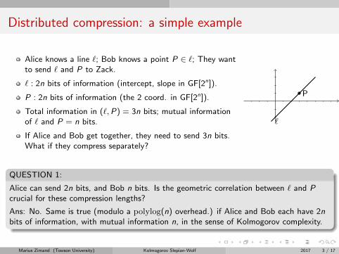
Alice knows a line `; Bob knows a point P ∈ `; They wantto send ` and P to Zack.
` : 2n bits of information (intercept, slope in GF[2n]).
P : 2n bits of information (the 2 coord. in GF[2n]).
Total information in (`,P) = 3n bits; mutual informationof ` and P = n bits.
If Alice and Bob get together, they need to send 3n bits.What if they compress separately?
`
P
Marius Zimand (Towson University) Kolmogorov Slepian-Wolf 2017 3 / 17
Distributed compression: a simple example
Alice knows a line `; Bob knows a point P ∈ `; They wantto send ` and P to Zack.
` : 2n bits of information (intercept, slope in GF[2n]).
P : 2n bits of information (the 2 coord. in GF[2n]).
Total information in (`,P) = 3n bits; mutual informationof ` and P = n bits.
If Alice and Bob get together, they need to send 3n bits.What if they compress separately?
`
P
QUESTION 1:
Alice can send 2n bits, and Bob n bits. Is the geometric correlation between ` and Pcrucial for these compression lengths?
Ans: No. Same is true (modulo a polylog(n) overhead.) if Alice and Bob each have 2nbits of information, with mutual information n, in the sense of Kolmogorov complexity.
Marius Zimand (Towson University) Kolmogorov Slepian-Wolf 2017 3 / 17

Distributed compression: a simple example
Alice knows a line `; Bob knows a point P ∈ `; They wantto send ` and P to Zack.
` : 2n bits of information (intercept, slope in GF[2n]).
P : 2n bits of information (the 2 coord. in GF[2n]).
Total information in (`,P) = 3n bits; mutual informationof ` and P = n bits.
If Alice and Bob get together, they need to send 3n bits.What if they compress separately?
`
P
QUESTION 2:
Can Alice send 1.5n bits, and Bob 1.5n bits? Can Alice send 1.74n bits, and Bob 1.26nbits?
Ans: Yes and Yes (modulo a polylog(n) overhead.)
Marius Zimand (Towson University) Kolmogorov Slepian-Wolf 2017 3 / 17

IT vs. AIT
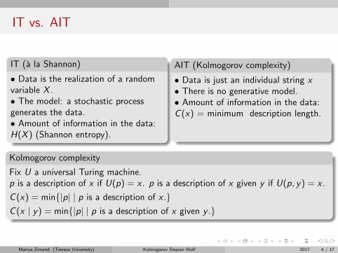
IT (a la Shannon)
• Data is the realization of a randomvariable X .• The model: a stochastic processgenerates the data.• Amount of information in the data:H(X ) (Shannon entropy).
AIT (Kolmogorov complexity)
• Data is just an individual string x• There is no generative model.• Amount of information in the data:C (x) = minimum description length.
0000000000000000
101101000110010
Kolmogorov complexity
Fix U a universal Turing machine.p is a description of x if U(p) = x . p is a description of x given y if U(p, y) = x .
C (x) = min{|p| | p is a description of x .}C (x | y) = min{|p| | p is a description of x given y .}
Marius Zimand (Towson University) Kolmogorov Slepian-Wolf 2017 4 / 17

IT vs. AIT
IT (a la Shannon)
• Data is the realization of a randomvariable X .• The model: a stochastic processgenerates the data.• Amount of information in the data:H(X ) (Shannon entropy).
AIT (Kolmogorov complexity)
• Data is just an individual string x• There is no generative model.• Amount of information in the data:C (x) = minimum description length.
0000000000000000
101101000110010
Kolmogorov complexity
Fix U a universal Turing machine.p is a description of x if U(p) = x . p is a description of x given y if U(p, y) = x .
C (x) = min{|p| | p is a description of x .}C (x | y) = min{|p| | p is a description of x given y .}
Marius Zimand (Towson University) Kolmogorov Slepian-Wolf 2017 4 / 17
Distributed compression (IT view): Slepian-Wolf Theorem
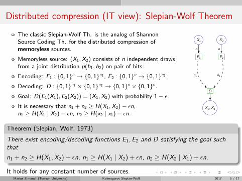
The classic Slepian-Wolf Th. is the analog of ShannonSource Coding Th. for the distributed compression ofmemoryless sources.
Memoryless source: (X1,X2) consists of n independent drawsfrom a joint distribution p(b1, b2) on pair of bits.
Encoding: E1 : {0, 1}n → {0, 1}n1 , E2 : {0, 1}n → {0, 1}n2 .Decoding: D : {0, 1}n1 × {0, 1}n2 → {0, 1}n × {0, 1}n.Goal: D(E1(X1),E2(X2)) = (X1,X2) with probability 1− ε.It is necessary that n1 + n2 ≥ H(X1,X2)− εn,n1 ≥ H(X1 | X2)− εn, n2 ≥ H(x2 | x1)− εn.
X2X1
E2E1
D
X1,X2
nn
n2n1
Theorem (Slepian, Wolf, 1973)
There exist encoding/decoding functions E1,E2 and D satisfying the goal suchthat
n1 + n2 ≥ H(X1,X2) + εn, n1 ≥ H(X1 | X2) + εn, n2 ≥ H(X2 | X1) + εn.
It holds for any constant number of sources.Marius Zimand (Towson University) Kolmogorov Slepian-Wolf 2017 5 / 17
Slepian-Wolf Th.: Some comments
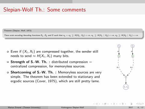
Theorem (Slepian, Wolf, 1973)
There exist encoding/decoding functions E1, E2 and D such that n1 + n2 ≥ H(X1, X2) + εn, n1 ≥ H(X1 | X2) + εn, n2 ≥ H(X2 | X1) + εn.
Even if (X1,X2) are compressed together, the sender stillneeds to send ≈ H(X1,X2) many bits.
Strength of S.-W. Th. : distributed compression =centralized compression, for memoryless sources.
Shortcoming of S.-W. Th. : Memoryless sources are verysimple. The theorem has been extended to stationary andergodic sources (Cover, 1975), which are still pretty lame.
X2X1
E2E1
D
X1, X2
nn
n2n1
Marius Zimand (Towson University) Kolmogorov Slepian-Wolf 2017 6 / 17

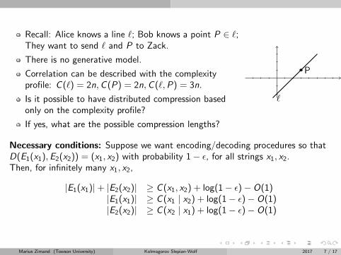
Recall: Alice knows a line `; Bob knows a point P ∈ `;They want to send ` and P to Zack.
There is no generative model.
Correlation can be described with the complexityprofile: C (`) = 2n,C (P) = 2n,C (`,P) = 3n.
Is it possible to have distributed compression basedonly on the complexity profile?
If yes, what are the possible compression lengths?
`
P
Necessary conditions: Suppose we want encoding/decoding procedures so thatD(E1(x1),E2(x2)) = (x1, x2) with probability 1− ε, for all strings x1, x2.Then, for infinitely many x1, x2,
|E1(x1)|+ |E2(x2)| ≥ C (x1, x2) + log(1− ε)− O(1)|E1(x1)| ≥ C (x1 | x2) + log(1− ε)− O(1)|E2(x2)| ≥ C (x2 | x1) + log(1− ε)− O(1)
Marius Zimand (Towson University) Kolmogorov Slepian-Wolf 2017 7 / 17

MAIN RESULT: Kolmogorov complexity version of theSlepian-Wolf Theorem
Theorem
There exist probabilistic poly.-time algorithms E1,E2
and algorithm D such that for all integers n1, n2 andn-bit strings x1, x2,if n1 + n2 ≥ C (x1, x2), n1 ≥ C (x1 | x2),n2 ≥ C (x2 | x1),
then
Ei on input (xi , ni ) outputs a string pi of lengthni + O(log3 n), for i = 1, 2,
D on input (p1, p2) outputs (x1, x2) withprobability 1− 1/n.
x2x1
E2E1
D
x1, x2
nn
n2n1
There is an analogous version for any constant number of sources.
Marius Zimand (Towson University) Kolmogorov Slepian-Wolf 2017 8 / 17

Some comments
Compression takes polynomial time. Decompression is slower than anycomputable function. This is unavoidable at this level of optimality(compression at close to minimum description length).
If we use time/space-bounded Kolmogorov complexity, decompression issomewhat better. For the line/point example, decompression is in linearspace.
Compression for individual strings is also done by Lempel-Ziv algorithms.They compress optimally for finite-state procedures. We compress at close tominimum description length.
At the high level, the proof follows the approach from a paper of AndreiRomashchenko (2005). Technical machinery is different.
The classical S.-W. Th. can be obtained from the Kolmogorov complexityversion (because if X is memoryless, H(X )− cε
√n ≤ C (X ) ≤ H(X ) + cε
√n
with prob. 1− ε).
The O(log3 n) overhead can be reduced to O(log n), but compression is nolonger in polynomial time.
Marius Zimand (Towson University) Kolmogorov Slepian-Wolf 2017 9 / 17

Proof sketch
Marius Zimand (Towson University) Kolmogorov Slepian-Wolf 2017 10 / 17

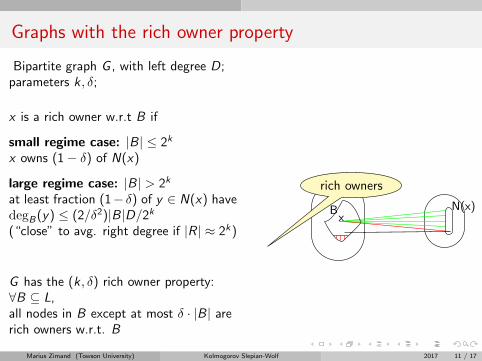
Graphs with the rich owner property
Bipartite graph G , with left degree D;parameters k , δ;
x is a rich owner w.r.t B if
small regime case: |B| ≤ 2k
x owns (1− δ) of N(x)
large regime case: |B| > 2k
at least fraction (1− δ) of y ∈ N(x) havedegB(y) ≤ (2/δ2)|B|D/2k
(“close” to avg. right degree if |R| ≈ 2k)
G has the (k, δ) rich owner property:∀B ⊆ L,all nodes in B except at most δ · |B| arerich owners w.r.t. B
xN(x)
x ’s neighbors
xN(x)B
xN(x)B
rich owners
poor owners
Marius Zimand (Towson University) Kolmogorov Slepian-Wolf 2017 11 / 17
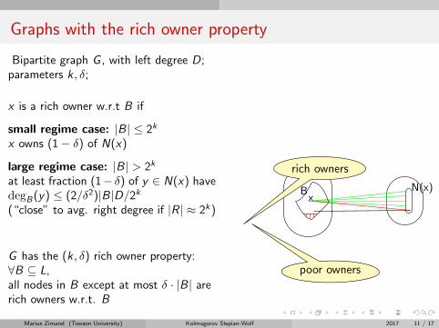
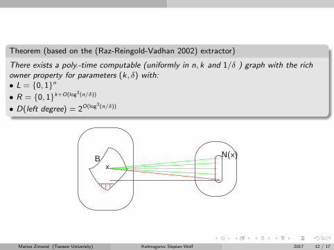
Theorem (based on the (Raz-Reingold-Vadhan 2002) extractor)
There exists a poly.-time computable (uniformly in n, k and 1/δ ) graph with the richowner property for parameters (k, δ) with:• L = {0, 1}n
• R = {0, 1}k+O(log3(n/δ))
• D(left degree) = 2O(log3(n/δ))
x
N(x)B
Marius Zimand (Towson University) Kolmogorov Slepian-Wolf 2017 12 / 17

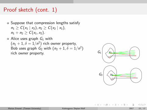
Proof sketch (cont. 1)
Suppose that compression lengths satisfyn1 ≥ C (x1 | x2), n2 ≥ C (x2 | x1),n1 + n2 ≥ C (x1, x2).
Alice uses graph G1 with(n1 + 1, δ = 1/n2) rich owner property,Bob uses graph G2 with (n2 + 1, δ = 1/n2)rich owner property.
Compression: Alice chooses p1 a randomneighbor of x1, Bob chooses p2 a randomneighbor of x2.
Decompression: Zack needs toreconstruct x1, x2 from p1, p2.
Idea: For i = 1, 2, find Bi in the “smallregime”, containing xi as a rich owner.Then with prob 1− δ, xi owns pi , so frompi we can reconstruct xi .
G1 x1
G2 x2
G1 x1 p1
G2 x2 p2
Marius Zimand (Towson University) Kolmogorov Slepian-Wolf 2017 13 / 17

Decompression - 1
Assume first that the decompressorknows the complexity profileC (x1),C (x2),C (x1, x2).
Case 1 (easy case): C (x2) ≤ n2.
Take B2 = {x | C (x) ≤ C (x2)}. B2 is inthe “small regime,” x2 is rich owner.
So, with prob 1− δ, x2 owns p2, so itcan be reconstructed from p2.
Take B1 = {x | C (x | x2) ≤ C (x1 | x2)}.B1 is in the “small regime,”, x1 is a richowner.
So, with prob 1− δ, x1 owns p1, so itcan be reconstructed from p1.
G1 x1 p1B1
G2 x2 p2B2
Marius Zimand (Towson University) Kolmogorov Slepian-Wolf 2017 14 / 17

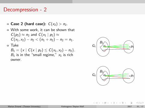
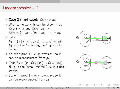
Decompression - 2
Case 2 (hard case): C (x2) > n2.
With some work, it can be shown thatC (p2) ≈ n2 and C (x1 | p2) ≈C (x1, x2)− n2 < (n1 + n2)− n2 = n1.
TakeB1 = {x | C (x | p2) ≤ C (x1, x2)− n2}.B1 is in the “small regime,” x1 is richowner.
So, with prob 1− δ, x1 owns p1, so itcan be reconstructed from p1.
Take B2 = {x | C (x | x1) ≤ C (x1 | x2)}.B2 is in the “small regime,”, x2 is a richowner.
So, with prob 1− δ, x2 owns p2, so itcan be reconstructed from p2.
G1 x1 p1B1
G2 x2 p2B2
Marius Zimand (Towson University) Kolmogorov Slepian-Wolf 2017 15 / 17

Decompression - 3
How to lift the assumption that the decompressor knows the complexityprofile C (x1),C (x2),C (x1, x2).
Try in parallel all possibilities for C (x1),C (x2),C (x1, x2). We run thedecompressor for each one till it finds the first neighbors of p1 and p2 in thecorresponding Bi -sets (Note: some may never find any neighbors).
For the right guess of the profile, p1 and p2 have unique neighbors in theBi -sets, and they are x1 and x2.
Using extra hashing, we can isolate x1 and x2 from the strings produced bythe parallel procedures with incorrect guesses. Cost of hashing: O(log n) bits,because there are O(n3) parallel procedures.
Marius Zimand (Towson University) Kolmogorov Slepian-Wolf 2017 16 / 17

Merci beaucoup.
Marius Zimand (Towson University) Kolmogorov Slepian-Wolf 2017 17 / 17


![Robust Distributed Source Coding with Arbitrary Number of ...jiaeee.com/article-1-151-fa.pdf · Distributed Source Coding (DSC) was introduced by Slepian and Wolf [1]. Multiterminal](https://static.fdocuments.in/doc/165x107/5e791557408573071a74159f/robust-distributed-source-coding-with-arbitrary-number-of-distributed-source.jpg)
![A generalised Quantum-Slepian Wolf - AQIS Confaqis-conf.org/2017/wp-content/uploads/2017/09/D5_05_5A01...The coding problem of Slepian and Wolf [1973] Quantum case: Techniques Conclusion](https://static.fdocuments.in/doc/165x107/5f2acad53361504ab60208bd/a-generalised-quantum-slepian-wolf-aqis-confaqis-conforg2017wp-contentuploads201709d5055a01.jpg)