Koller & Friedman Chapters (handed out): Chapter 11 (short...
84
1 Bayesian Networks – Structure Learning (cont.) Machine Learning – 10701/15781 Carlos Guestrin Carnegie Mellon University April 3 rd , 2006 Koller & Friedman Chapters (handed out): Chapter 11 (short) Chapter 12: 12.1, 12.2, 12.3 (covered in the beginning of semester) 12.4 (Learning parameters for BNs) Chapter 13: 13.1, 13.3.1, 13.4.1, 13.4.3 (basic structure learning) Learning BN tutorial (class website): ftp://ftp.research.microsoft.com/pub/tr/tr-95-06.pdf TAN paper (class website): http://www.cs.huji.ac.il/~nir/Abstracts/FrGG1.html
Transcript of Koller & Friedman Chapters (handed out): Chapter 11 (short...

1
Bayesian Networks –Structure Learning (cont.)
Machine Learning – 10701/15781Carlos GuestrinCarnegie Mellon University
April 3rd, 2006
Koller & Friedman Chapters (handed out):Chapter 11 (short)Chapter 12: 12.1, 12.2, 12.3 (covered in the beginning of semester)
12.4 (Learning parameters for BNs)Chapter 13: 13.1, 13.3.1, 13.4.1, 13.4.3 (basic structure learning)
Learning BN tutorial (class website):ftp://ftp.research.microsoft.com/pub/tr/tr-95-06.pdf
TAN paper (class website):http://www.cs.huji.ac.il/~nir/Abstracts/FrGG1.html
2
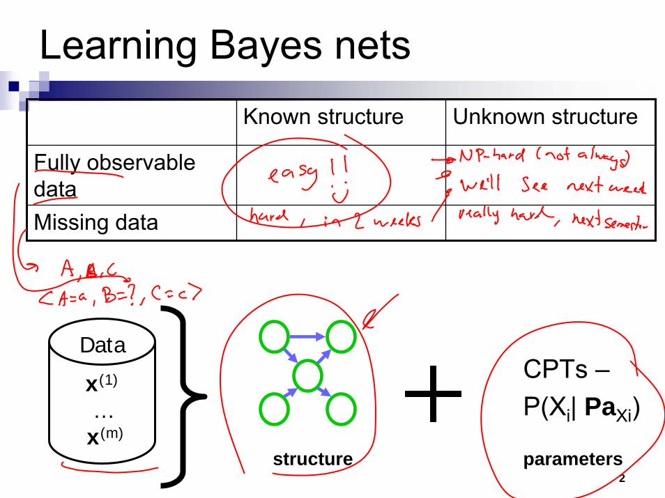
Learning Bayes netsKnown structure Unknown structure
Fully observable dataMissing data
x(1)
…x(m)
Data
structure parameters
CPTs –P(Xi| PaXi)
3
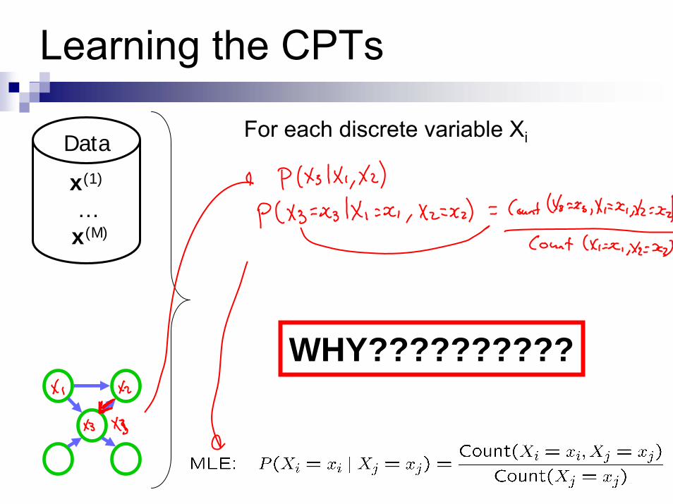
Learning the CPTs
x(1)
…x(M)
DataFor each discrete variable Xi
WHY??????????

4
Information-theoretic interpretation of maximum likelihood
Given structure, log likelihood of data:
Flu Allergy
Sinus
Headache Nose

5
Maximum likelihood (ML) for learning BN structure
Data
<x1(1),…,xn
(1)>…
<x1(M),…,xn
(M)>
Flu Allergy
Sinus
Headache Nose
Possible structures Score structureLearn parametersusing ML

6
Information-theoretic interpretation of maximum likelihood 2
Given structure, log likelihood of data:
Flu Allergy
Sinus
Headache Nose

7
Information-theoretic interpretation of maximum likelihood 3
Given structure, log likelihood of data:
Flu Allergy
Sinus
Headache Nose

8
Mutual information → Independence tests
Statistically difficult task!Intuitive approach: Mutual information
Mutual information and independence:Xi and Xj independent if and only if I(Xi,Xj)=0
Conditional mutual information:

9
Decomposable score
Log data likelihood

10
Scoring a tree 1: equivalent trees

11
Scoring a tree 2: similar trees

12
Chow-Liu tree learning algorithm 1
For each pair of variables Xi,XjCompute empirical distribution:
Compute mutual information:
Define a graphNodes X1,…,Xn
Edge (i,j) gets weight

13
Chow-Liu tree learning algorithm 2
Optimal tree BNCompute maximum weight spanning treeDirections in BN: pick any node as root, breadth-first-search defines directions

14
Can we extend Chow-Liu 1
Tree augmented naïve Bayes (TAN) [Friedman et al. ’97]
Naïve Bayes model overcounts, because correlation between features not consideredSame as Chow-Liu, but score edges with:
15
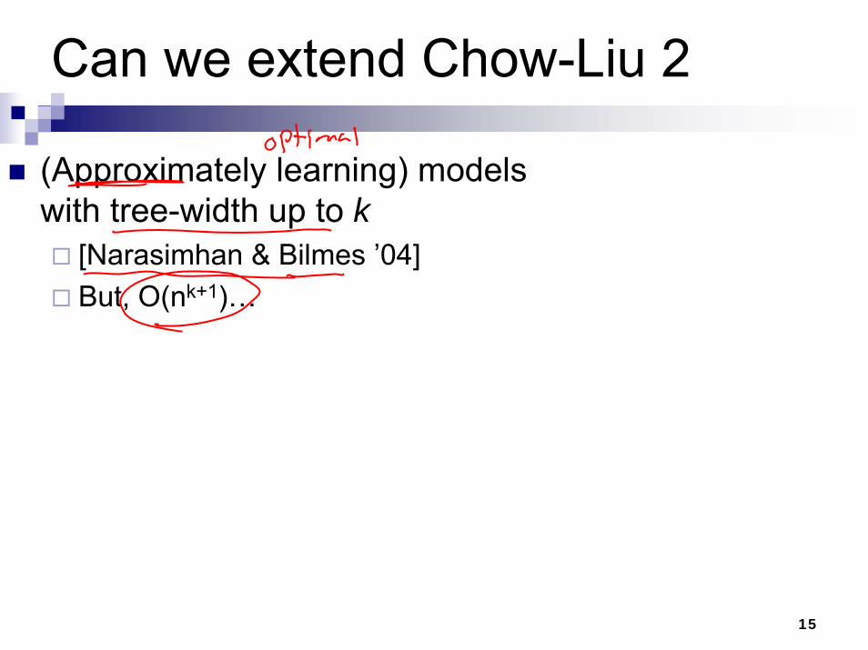
Can we extend Chow-Liu 2
(Approximately learning) models with tree-width up to k
[Narasimhan & Bilmes ’04]But, O(nk+1)…

16
Scoring general graphical models –Model selection problemWhat’s the best structure?
Data
<x_1^{(1)},…,x_n^{(1)}>…
<x_1^{(m)},…,x_n^{(m)}>
Flu Allergy
Sinus
Headache Nose
The more edges, the fewer independence assumptions,the higher the likelihood of the data, but will overfit…

17
Maximum likelihood overfits!
Information never hurts:
Adding a parent always increases score!!!

18
Bayesian score avoids overfitting
Given a structure, distribution over parameters
Difficult integral: use Bayes information criterion (BIC) approximation (equivalent as M→∞)
Note: regularize with MDL scoreBest BN under BIC still NP-hard

19
How many graphs are there?

20
Structure learning for general graphs
In a tree, a node only has one parent
Theorem:The problem of learning a BN structure with at most dparents is NP-hard for any (fixed) d≥2
Most structure learning approaches use heuristicsExploit score decomposition(Quickly) Describe two heuristics that exploit decomposition in different ways

21
Learn BN structure using local search
Score using BICLocal search,possible moves:• Add edge• Delete edge• Invert edge
Starting from Chow-Liu tree

22
What you need to know about learning BNsLearning BNs
Maximum likelihood or MAP learns parametersDecomposable scoreBest tree (Chow-Liu)Best TANOther BNs, usually local search with BIC score

23
Unsupervised learning or Clustering –K-meansGaussian mixture modelsMachine Learning – 10701/15781Carlos GuestrinCarnegie Mellon University
April 3rd, 2006

24
Some Data
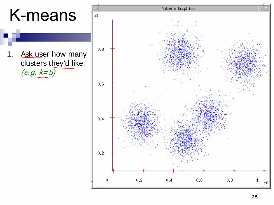
K-means
25
1. Ask user how many clusters they’d like. (e.g. k=5)

26
K-means
1. Ask user how many clusters they’d like. (e.g. k=5)
2. Randomly guess k cluster Center locations

27
K-means
1. Ask user how many clusters they’d like. (e.g. k=5)
2. Randomly guess k cluster Center locations
3. Each datapoint finds out which Center it’s closest to. (Thus each Center “owns”a set of datapoints)

28
K-means
1. Ask user how many clusters they’d like. (e.g. k=5)
2. Randomly guess k cluster Center locations
3. Each datapoint finds out which Center it’s closest to.
4. Each Center finds the centroid of the points it owns

29
K-means
1. Ask user how many clusters they’d like. (e.g. k=5)
2. Randomly guess k cluster Center locations
3. Each datapoint finds out which Center it’s closest to.
4. Each Center finds the centroid of the points it owns…
5. …and jumps there
6. …Repeat until terminated!
30
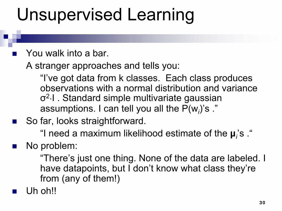
Unsupervised Learning
You walk into a bar.A stranger approaches and tells you:
“I’ve got data from k classes. Each class produces observations with a normal distribution and variance σ2·I . Standard simple multivariate gaussian assumptions. I can tell you all the P(wi)’s .”
So far, looks straightforward.“I need a maximum likelihood estimate of the µi’s .“
No problem:“There’s just one thing. None of the data are labeled. I have datapoints, but I don’t know what class they’re from (any of them!)
Uh oh!!

31
Gaussian Bayes Classifier Reminder
)()()|()|(
xxx
piyPiypiyP ==
==
( ) ( )
)(21exp
||||)2(1
)|(2/12/
x
µxΣµxΣx
p
piyP
iikiT
iki
m ⎥⎦⎤
⎢⎣⎡ −−−
==π
How do we deal with that?

32
Predicting wealth from age

33
Predicting wealth from age

34
Learning modelyear , mpg ---> maker
⎟⎟⎟⎟⎟
⎠
⎞
⎜⎜⎜⎜⎜
⎝
⎛
=
mmm
m
m
221
222
12
11212
σσσ
σσσσσσ
L
MOMM
L
L
Σ

35
General: O(m2)parameters
⎟⎟⎟⎟⎟
⎠
⎞
⎜⎜⎜⎜⎜
⎝
⎛
=
mmm
m
m
221
222
12
11212
σσσ
σσσσσσ
L
MOMM
L
L
Σ

36
Aligned: O(m)parameters
⎟⎟⎟⎟⎟⎟⎟⎟
⎠
⎞
⎜⎜⎜⎜⎜⎜⎜⎜
⎝
⎛
=
−
m
m
2
12
32
22
12
00000000
000000000000
σσ
σσ
σ
L
L
MMOMMM
L
L
L
Σ

37
Aligned: O(m)parameters
⎟⎟⎟⎟⎟⎟⎟⎟
⎠
⎞
⎜⎜⎜⎜⎜⎜⎜⎜
⎝
⎛
=
−
m
m
2
12
32
22
12
00000000
000000000000
σσ
σσ
σ
L
L
MMOMMM
L
L
L
Σ

38
Spherical: O(1)cov parameters
⎟⎟⎟⎟⎟⎟⎟⎟
⎠
⎞
⎜⎜⎜⎜⎜⎜⎜⎜
⎝
⎛
=
2
2
2
2
2
00000000
000000000000
σσ
σσ
σ
L
L
MMOMMM
L
L
L
Σ

39
Spherical: O(1)cov parameters
⎟⎟⎟⎟⎟⎟⎟⎟
⎠
⎞
⎜⎜⎜⎜⎜⎜⎜⎜
⎝
⎛
=
2
2
2
2
2
00000000
000000000000
σσ
σσ
σ
L
L
MMOMMM
L
L
L
Σ

40
Next… back to Density Estimation
What if we want to do density estimation with multimodal or clumpy data?
41
The GMM assumption
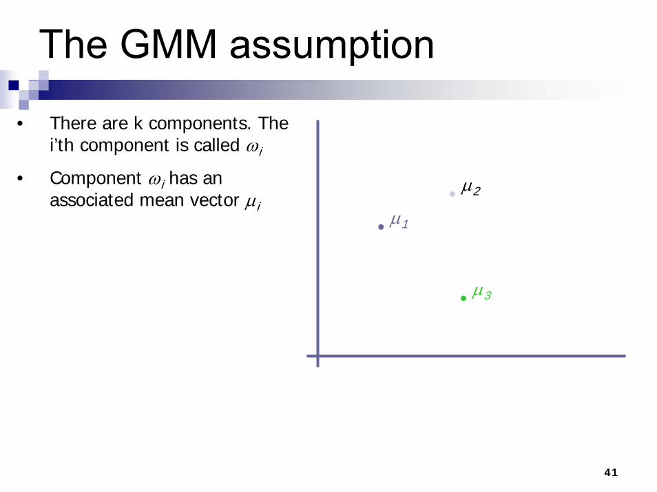
• There are k components. The i’th component is called ωi
• Component ωi has an associated mean vector µi
µ1
µ2
µ3

42
The GMM assumption
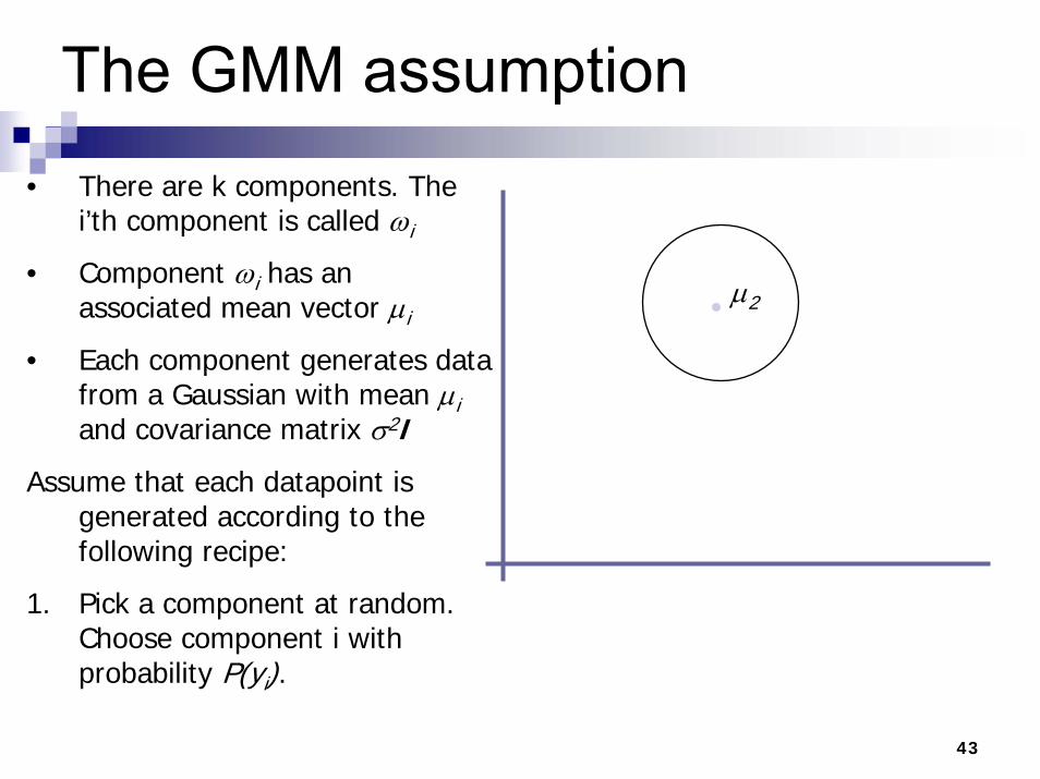
• There are k components. The i’th component is called ωi
• Component ωi has an associated mean vector µi
• Each component generates data from a Gaussian with mean µi and covariance matrix σ2I
Assume that each datapoint is generated according to the following recipe:
µ1
µ2
µ3
43
The GMM assumption• There are k components. The
i’th component is called ωi
• Component ωi has an associated mean vector µi
• Each component generates data from a Gaussian with mean µi and covariance matrix σ2I
Assume that each datapoint is generated according to the following recipe:
1. Pick a component at random. Choose component i with probability P(yi).
µ2

44
The GMM assumption• There are k components. The
i’th component is called ωi
• Component ωi has an associated mean vector µi
• Each component generates data from a Gaussian with mean µi and covariance matrix σ2I
Assume that each datapoint is generated according to the following recipe:
1. Pick a component at random. Choose component i with probability P(yi).
2. Datapoint ~ N(µi, σ2I )
µ2
x

45
The General GMM assumption
µ1
µ2
µ3
• There are k components. The i’th component is called ωi
• Component ωi has an associated mean vector µi
• Each component generates data from a Gaussian with mean µi and covariance matrix Σi
Assume that each datapoint is generated according to the following recipe:
1. Pick a component at random. Choose component i with probability P(yi).
2. Datapoint ~ N(µi, Σi )

46
Unsupervised Learning:not as hard as it looks
Sometimes easy
Sometimes impossible
and sometimes in between
IN CASE YOU’RE WONDERING WHAT THESE DIAGRAMS ARE, THEY SHOW 2-d UNLABELED DATA (XVECTORS) DISTRIBUTED IN 2-d SPACE. THE TOP ONE HAS THREE VERY CLEAR GAUSSIAN CENTERS

47
Computing likelihoods in supervised learning caseWe have y1,x1 , y2,x2 , … yN,xN
Learn P(y1) P(y2) .. P(yk)Learn σ, µ1,…, µk
By MLE: P(y1,x1 , y2,x2 , … yN,xN |µi, … µk , σ)

48
Computing likelihoods in unsupervised caseWe have x1 , x2 , … xN
We know P(y1) P(y2) .. P(yk)We know σ
P(x|yi, µi, … µk) = Prob that an observation from class yiwould have value x given class means µ1… µx
Can we write an expression for that?

49
likelihoods in unsupervised case
We have x1 x2 … xnWe have P(y1) .. P(yk). We have σ.We can define, for any x , P(x|yi , µ1, µ2 .. µk)
Can we define P(x | µ1, µ2 .. µk) ?
Can we define P(x1, x1, .. xn | µ1, µ2 .. µk) ?
[YES, IF WE ASSUME THE X1’S WERE DRAWN INDEPENDENTLY]

50
Unsupervised Learning:Mediumly Good NewsWe now have a procedure s.t. if you give me a guess at µ1, µ2 .. µk,
I can tell you the prob of the unlabeled data given those µ‘s.
Suppose x‘s are 1-dimensional.
There are two classes; w1 and w2
P(y1) = 1/3 P(y2) = 2/3 σ = 1 .
There are 25 unlabeled datapoints
x1 = 0.608x2 = -1.590x3 = 0.235x4 = 3.949
:x25 = -0.712
(From Duda and Hart)

51
Duda & Hart’s ExampleWe can graph the
prob. dist. function of data given our µ1 and µ2estimates.
We can also graph the true function from which the data was randomly generated.
• They are close. Good.
• The 2nd solution tries to put the “2/3” hump where the “1/3” hump should go, and vice versa.
• In this example unsupervised is almost as good as supervised. If the x1 .. x25 are given the class which was used to learn them, then the results are (µ1=-2.176, µ2=1.684). Unsupervised got (µ1=-2.13, µ2=1.668).

52
Graph of log P(x1, x2 .. x25 | µ1, µ2 )
against µ1 (→) and µ2 (↑)
Max likelihood = (µ1 =-2.13, µ2 =1.668)
Local minimum, but very close to global at (µ1 =2.085, µ2 =-1.257)*
* corresponds to switching y1 with y2.
Duda & Hart’s Example
µ1
µ2

53
Finding the max likelihood µ1,µ2..µk
We can compute P( data | µ1,µ2..µk)How do we find the µi‘s which give max. likelihood?
The normal max likelihood trick:Set ∂ log Prob (….) = 0
∂ µi
and solve for µi‘s.# Here you get non-linear non-analytically-solvable equations
Use gradient descentSlow but doable
Use a much faster, cuter, and recently very popular method…

54
Expectation Maximalization

55
The E.M. Algorithm
We’ll get back to unsupervised learning soon.But now we’ll look at an even simpler case with hidden information.The EM algorithm
Can do trivial things, such as the contents of the next few slides.An excellent way of doing our unsupervised learning problem, as we’ll see.Many, many other uses, including inference of Hidden Markov Models (future lecture).
DETOUR

56
Silly ExampleLet events be “grades in a class”
w1 = Gets an A P(A) = ½w2 = Gets a B P(B) = µw3 = Gets a C P(C) = 2µw4 = Gets a D P(D) = ½-3µ
(Note 0 ≤ µ ≤1/6)Assume we want to estimate µ from data. In a given class there were
a A’sb B’sc C’sd D’s
What’s the maximum likelihood estimate of µ given a,b,c,d ?

57
Silly Example
Let events be “grades in a class”w1 = Gets an A P(A) = ½w2 = Gets a B P(B) = µw3 = Gets a C P(C) = 2µw4 = Gets a D P(D) = ½-3µ
(Note 0 ≤ µ ≤1/6)Assume we want to estimate µ from data. In a given class there were
a A’sb B’sc C’sd D’s
What’s the maximum likelihood estimate of µ given a,b,c,d ?

58
Trivial StatisticsP(A) = ½ P(B) = µ P(C) = 2µ P(D) = ½-3µP( a,b,c,d | µ) = K(½)a(µ)b(2µ)c(½-3µ)d
log P( a,b,c,d | µ) = log K + alog ½ + blog µ + clog 2µ + dlog (½-3µ)
( )
101µ likeMax
got class if So6
µ likemax Gives
0µ32/1
3µ2
2µµ
LogP
0µ
LogP SET µ, LIKE MAX FOR
=
+++
=
=−
−+=∂
∂
=∂
∂
dcbcb
dcb
A B C D
14 6 9 10
Boring, but true!

59
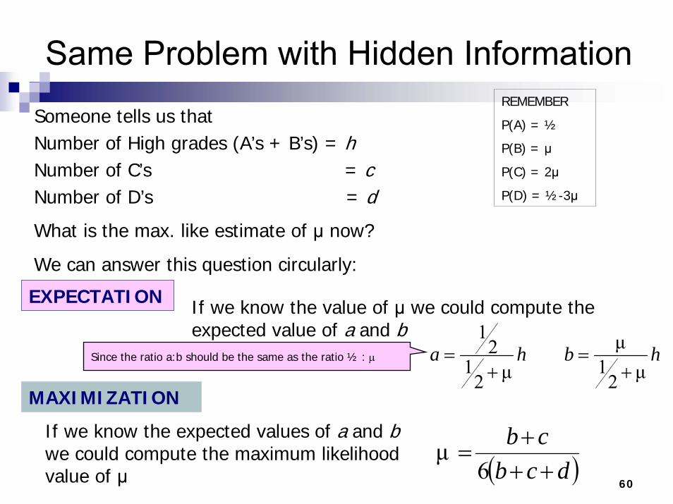
Same Problem with Hidden InformationREMEMBER
P(A) = ½
P(B) = µ
P(C) = 2µ
P(D) = ½-3µ
Someone tells us thatNumber of High grades (A’s + B’s) = hNumber of C’s = cNumber of D’s = d
What is the max. like estimate of µ now?
60
Same Problem with Hidden InformationREMEMBER
P(A) = ½
P(B) = µ
P(C) = 2µ
P(D) = ½-3µ
Someone tells us thatNumber of High grades (A’s + B’s) = hNumber of C’s = cNumber of D’s = d
What is the max. like estimate of µ now?
We can answer this question circularly:
hbhaµ2
1µ
µ21
21
+=
+=
EXPECTATION
MAXIMIZATION
If we know the value of µ we could compute the expected value of a and b
Since the ratio a:b should be the same as the ratio ½ : µ
If we know the expected values of a and bwe could compute the maximum likelihood value of µ ( )dcb
cb++
+=
6 µ

61
E.M. for our Trivial Problem REMEMBER
P(A) = ½
P(B) = µ
P(C) = 2µ
P(D) = ½-3µWe begin with a guess for µWe iterate between EXPECTATION and MAXIMALIZATION to improve ourestimates of µ and a and b.
Define µ(t) the estimate of µ on the t’th iterationb(t) the estimate of b on t’th iteration
[ ]
( )( )( )
( )tbdctb
ctbt
tbt
htb
given µ ofest likemax 6
)1(µ
)(µ|)(µ2
1µ(t) )(
guess initial )0(µ
=++
+=+
Ε=+
=
=
E-step
M-step
Continue iterating until converged.Good news: Converging to local optimum is assured.Bad news: I said “local” optimum.

62
E.M. ConvergenceConvergence proof based on fact that Prob(data | µ) must increase or remain same between each iteration [NOT OBVIOUS]
But it can never exceed 1 [OBVIOUS]
So it must therefore converge [OBVIOUS]
In our example, suppose we had
h = 20c = 10d = 10
µ(0) = 0
t µ(t) b(t)
0 0 0
1 0.0833 2.857
2 0.0937 3.158
3 0.0947 3.185
4 0.0948 3.187
5 0.0948 3.187
6 0.0948 3.187
Convergence is generally linear: error decreases by a constant factor each time step.

63
Back to Unsupervised Learning of GMMs
Remember:We have unlabeled data x1 x2 … xRWe know there are k classesWe know P(y1) P(y2) P(y3) … P(yk)We don’t know µ1 µ2 .. µk
We can write P( data | µ1…. µk)
( )
( )
( ) ( )
( ) ( )∏∑
∏∑
∏
= =
= =
=
⎟⎠⎞
⎜⎝⎛ −−=
=
=
=
R
i
k
jjji
R
i
k
jjkji
R
iki
kR
yx
ywx
x
xx
1 1
22
1 11
11
11
Pµσ21expK
Pµ...µ,p
µ...µp
µ...µ...p

64
E.M. for GMMs
( )
( )
( )∑
∑
=
==
=∂∂
R
ikij
i
R
ikij
j
ki
xyP
xxyP
11
11
1
µ...µ,
µ...µ, µ
j, eachfor ,likelihoodFor Max " :into thisrnsalgebra tucrazy n' wild'Some
0µ...µdataobPrlogµ
know welikelihoodFor Max
This is n nonlinear equations in µj’s.”
…I feel an EM experience coming on!!
If, for each xi we knew that for each wj the prob that µj was in class yj isP(yj|xi,µ1…µk) Then… we would easily compute µj.
If we knew each µj then we could easily compute P(yj|xi,µ1…µk) for each yjand xi.
See
http://www.cs.cmu.edu/~awm/doc/gmm-algebra.pdf
65
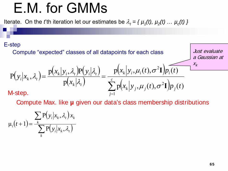
E.M. for GMMsIterate. On the t’th iteration let our estimates be λt = { µ1(t), µ2(t) … µc(t) }
E-stepCompute “expected” classes of all datapoints for each class
( ) ( ) ( )( )
( )( )∑
=
== c
jjjjk
iiik
tk
titiktki
tptyx
tptyxx
yyxxy
1
2
2
)(),(,p
)(),(,pp
P,p,P
I
I
σµ
σµλ
λλλ
M-step. Compute Max. like µ given our data’s class membership distributions
( )( )( )∑
∑=+
ktki
kk
tki
i xy
xxyt
λ
λ
,P
,P1µ
Just evaluate a Gaussian at xk

66
E.M. Convergence
This algorithm is REALLY USED. And in high dimensional state spaces, too. E.G. Vector Quantization for Speech Data
• Your lecturer will (unless out of time) give you a nice intuitive explanation of why this rule works.
• As with all EM procedures, convergence to a local optimum guaranteed.

E.M. for General GMMs
67
Iterate. On the t’th iteration let our estimates be
λt = { µ1(t), µ2(t) … µc(t), Σ1(t), Σ2(t) … Σc(t), p1(t), p2(t) … pc(t) }
E-stepCompute “expected” classes of all datapoints for each class
( ) ( ) ( )( )
( )( )∑
=
Σ
Σ== c
jjjjjk
iiiik
tk
titiktki
tpttyx
tpttyxx
yyxxy
1
)()(),(,p
)()(),(,pp
P,p,P
µ
µλ
λλλ
M-step. Compute Max. like µ given our data’s class membership distributions
pi(t) is shorthand for estimate of P(yi)on t’th iteration
( )( )( )∑
∑=+
ktki
kk
tki
i xy
xxyt
λ
λ
,P
,P1µ ( )
( ) ( )[ ] ( )[ ]
( )∑∑ +−+−
=+Σ
ktki
Tikik
ktki
i xy
txtxxyt
λ
µµλ
,P
11 ,P1
( )( )
R
xytp k
tki
i
∑=+
λ,P1 R = #records
Just evaluate a Gaussian at xk

68
Advance apologies: in Black and White this example will be
incomprehensible
Gaussian Mixture Example: Start

69
After first iteration

70
After 2nd iteration

71
After 3rd iteration

72
After 4th iteration

73
After 5th iteration

74
After 6th iteration

75
After 20th iteration
76
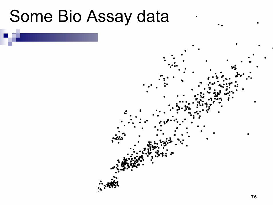
Some Bio Assay data

77
GMM clustering of the assay data

78
Resulting Density Estimator

79
Three classes of assay(each learned with it’s own mixture model)

80
Resulting Bayes Classifier

81
Resulting Bayes Classifier, using posterior probabilities to alert about ambiguity and anomalousness
Yellow means anomalous
Cyan means ambiguous

82
Final Comments
Remember, E.M. can get stuck in local minima, and empirically it DOES.Our unsupervised learning example assumed P(yi)’s known, and variances fixed and known. Easy to relax this.It’s possible to do Bayesian unsupervised learning instead of max. likelihood.
83
What you should know
How to “learn” maximum likelihood parameters (locally max. like.) in the case of unlabeled data.Be happy with this kind of probabilistic analysis.Understand the two examples of E.M. given in these notes.

84
Acknowledgements
K-means & Gaussian mixture models presentation derived from excellent tutorial by Andrew Moore:
http://www.autonlab.org/tutorials/K-means Applet:
http://www.elet.polimi.it/upload/matteucc/Clustering/tutorial_html/AppletKM.html
Gaussian mixture models Applet:http://www.neurosci.aist.go.jp/%7Eakaho/MixtureEM.html