Knowledge Diffusion in the Workplace∗

Kyle Herkenhoff Jeremy Lise Guido Menzio Gordon Phillips

July 14, 2018

Preliminary

Abstract

We develop a theory of teams to measure the way knowledge diffuses across work-

ers. We build a frictional sorting framework with production complementarities which

allows for workers to influence each other’s knowledge. We estimate the model using

matched employer-employee data for the U.S. Our estimates imply strong peer effects.

With strong peer effects, both the decentralized economy and planner optimally pair

low human capital workers with high human capital workers. We show that at least

16% of measured “mismatch” (pairing high and low types) in the U.S. economy is

due to peer effects. Lastly, peer effects and worker mobility are equally important

determinants of output, with each factor accounting for roughly 1/6 of U.S. GDP.

∗Herkenhoff: University of Minnesota. Lise: University of Minnesota. Menzio: University of Penn-

sylvania, & NBER. Phillips: Dartmouth College, University of Maryland, & NBER. We thank seminar

participants at Aarhus, Atlanta Fed, Carnegie-Mellon, FGV, IIES, Oslo, SAET, SaM, San Francisco Fed,

and the SED. We are especially indebted to Carlos Henrique Leite Corseuil for his help and comments. Any

opinions and conclusions expressed herein are those of the author(s) and do not necessarily represent the

views of the U.S. Census Bureau. All results have been reviewed to ensure that no confidential information

is disclosed. This research uses data from the Census Bureau’s Longitudinal Employer Household Dynamics

Program, which was partially supported by the following National Science Foundation Grants SES-9978093,

SES-0339191 and ITR-0427889; National Institute on Aging Grant AG018854; and grants from the Alfred

P. Sloan Foundation.

1

1 Introduction

How does knowledge diffuse across workers? In this paper, we develop a model which allows

us to estimate the importance of peer effects and worker mobility for knowledge diffusion.

By doing so, we contribute to a fast and growing literature on knowledge diffusion (inter

alia Jovanovic and Rob [1989], Eeckhout and Jovanovic [2002], Luttmer [2014], Lucas and

Moll [2014], Perla and Tonetti [2014], Heggedal, Moen, and Preugschat [2017]), and the

relatively large existing literature on peer effects (inter alia Mas and Moretti [2009], Nix

[2015], Cornelissen, Dustmann, and Schonberg [2016]).

Our theoretic contribution is to develop a model of teams with peer effects and on-the-job

search. We build on a relatively small class of existing sorting models with dynamic types

(e.g. Anderson and Smith [2010], Chade and Eeckhout [2013], Lentz and Roys [2015], Lise

and Postel-Vinay [2015], and Herkenhoff, Phillips, and Cohen-Cole [2016]) by introducing

dynamic types that evolve as a function of coworker characteristics in a search environment.

The firm ‘type’ is no longer an exogenous draw from a distribution as it is commonly modeled

in the frictional assignment literature (inter alia Shimer and Smith [2000], Hagedorn, Law,

and Manovskii [2012]), but instead it is an evolving function of the set of coworkers. In our

framework, workers spread knowledge through two channels: (i) through interactions with

existing team members, or (ii) job transitions in which a worker leaves for another firm,

either directly through on-the-job search or indirectly through a spell of unemployment, and

the worker transfers whatever knowledge they have to new coworkers.

Our quantitative contribution is to estimate the sources of knowledge diffusion using

the structure of our model and matched employer-employee data from the Longitudinal

Employer-Household Dynamics (LEHD) database. The main challenge when estimating

peer effects in our model is that existing empirical methods, such as those in Nix [2015]

and Cornelissen et al. [2016], impose fixed-type assumptions that are inconsistent with our

model assumptions. Likewise, many methods used to estimate the degree of sorting such as

Abowd, Kramarz, and Margolis [1999], Hagedorn et al. [2012], Bonhomme, Lamadon, and

Manresa [2014], and Borovickova and Shimer [2017] rely on fixed type assumptions.

We estimate the degree of learning and sorting by using the structure of our model in

conjunction with the LEHD. Our approach is to indirectly infer the model’s sorting and

learning parameters from three moments in the LEHD, that, when viewed through the lens

of our model, directly inform sorting and learning. The first moment exploits the fact that

learning has unique predictions about job mobility and the wages of coworkers. Through the

2

lens of the model, the worker’s wage is a noisy proxy of an individual’s type and the coworker’s

wage is a noisy proxy of the coworker’s type. With strong production complementarity and

no learning, the further a worker’s wage is from their coworker’s wage, the more likely they

are to switch employers in search of a better match. With strong learning and no production

complementarity, the further a worker’s wage is from their coworker’s wage, the less likely

they are to switch employers because they are either learning or teaching their coworker.

The second moment we use to disentangle learning and sorting is based on the correlation

between an individual’s wage and their previous coworkers’ wages. To parse out sticky-wages,

built-up rents, and other forces which drive a wedge between a worker’s type and their true

productivity, we focus on individuals who separate, experience a spell of unemployment, and

then find a new job. We refer to this as an ‘EUE’ transition. As sorting improves, coworker

wages become a stronger predictor of the worker’s type, and thus coworker wages become

better predictors of future individual wages. As learning improves, the same is true. Our

last moment is the share of wage variance that is between firms. Since there are multiple

workers at a firm in our model, our framework has a concept of within-firm and between-firm

wage variance. As production complementarities increase, between-firm wage variance grows

relative to within-firm wage variance. Conversely, as learning becomes more important, the

within-firm wage variance share grows. The fact that learning and sorting move two of our

moments in opposing directions and one of our moments in the same direction allows us to

pin down both the level and relative importance of peer effects and worker complementarity.

Our estimated parameters imply very strong degrees of both skill complementarity and

peer effects. We then use the estimated model to measure the relative importance of peer

effects and worker mobility for U.S. output. Our first finding is that eliminating peer effects

would lower output by 16.3%, even though standard measures of sorting improve. Without

learning, fewer workers reach the highest skill level since low-type workers can no longer learn

from their more-skilled peers. When learning is shutdown there are no incentives to generate

schools (a school is a pairing of a low and high type worker), and so more same-type matches

arise in equilibrium. As a side-effect, sorting improves. Sorting, measured by the Spearman

rank correlation coefficient, increases by 25% when learning is eliminated, going from .4 to .5.

Our estimates imply that learning accounts for at least 16% of measured ‘mismatch.’ This

is not to say that learning is actually causing any mismatch by incentivizing pairings of high

and low-type workers (e.g. forming schools). We demonstrate that the planner’s solution

features 38% of individuals in schools, 4 percentage points more than in the decentralized

economy.

3

Eliminating endogenous reallocation of workers between jobs, but still allowing workers to

learn from each other, also reduces output by 15.7%. There are two mechanisms generating

this result: (i) fewer teams are formed since workers can no longer search for productive

partners on-the-job, and (ii) with fewer teams, human capital diffuses more slowly. The net

effect is that worker mobility explains roughly 1/6 of U.S. GDP, while shutting down both

worker mobility and learning simultaneously reduces output by nearly 1/3.

Lastly, the decentralized equilibrium is inefficient. Firms are not fully compensated

for educating workers. Because wages are determined via Nash-Bargaining and Bertrand

competition as in Cahuc et al. [2006], firms only receive a fraction of the social surplus they

generate by educating their workers. As a result, there are too few schools in the decentralized

equilibrium relative to the social planner’s problem. By generating more schools, we find

that the social planner’s allocation would increase output by 4 percentage points.

The paper proceeds as follows. Section 2 discusses the related literature in more detail.

Section 3 includes the model. Section 4 describes the calibration. Section 5 illustrates the

main knowledge diffusion decomposition, and Section 6 compares the decentralized economy

the to planner’s solution. Section 7 concludes.

2 Related Literature

Our model contributes to the literature on sorting with dynamic types (e.g. see the survey

of sorting models in Chade, Eeckhout, and Smith [2017]). Anderson and Smith [2010] and

Anderson [2015] consider frictionless assignment models with partner-dependent dynamic

types. Related work by Jovanovic [2014] extends Anderson and Smith [2010] to allow for

growth. In frictional sorting models, an equally sparse set of papers allow for one-sided

dynamic types, including Chade and Eeckhout [2013], Lentz and Roys [2015] and Lise and

Postel-Vinay [2015]. Lentz and Roys [2015] develop a search and matching model in which

firms can invest in worker training; thus, the worker type fluctuates over time and is de-

termined by the firm’s choices. Lise and Postel-Vinay [2015] allow firms to influence the

vector of worker skills. Recent work by Herkenhoff et al. [2016] allows worker human capital

and firm capital to fluctuate over the course of a match, but the firm investment choice

does not affect the worker’s human capital. Lastly, Heggedal et al. [2017] model firm in-

novation choices in the presence of worker mobility in a two-period economy. Their focus

is on theoretically characterizing welfare gains and losses from various innovation-related

4

interventions in the decentralized economy. Our paper also relates to the theoretic literature

on knowledge diffusion through interaction, (e.g. Jovanovic and Rob [1989], Eeckhout and

Jovanovic [2002], Luttmer [2014], Lucas and Moll [2014], Perla and Tonetti [2014], Chiu

et al. [2017]) and a growing literature that models knowledge diffusion through trade, (e.g.

Monge-Naranjo [2012], Buera and Oberfield [2016]). Relative to these existing frameworks,

our contribution is to build a frictional sorting model with peer affects and job-to-job flows.

In terms of empirics, Stoyanov and Zubanov [2012] and Serafinelli [2015] provide recent

summaries of the empirical literature on worker mobility and firm productivity. These stud-

ies, as well as the majority of other papers in this literature, find that poaching high-wage

workers has a large positive impact on firm productivity, although the mechanisms are not

well understood.1 In the peer-effects literature, recent work by Cornelissen et al. [2016] and

Nix [2015] rely on long panel dimensions of administrative data to disentangle worker traits,

such as ability, from coworker peer-effects.2 Both Cornelissen et al. [2016] and Nix [2015] find

significant, but relatively small, coworker influence on future wages. Lastly, recent empirical

work by Brooks, Donovan, and Johnson [2017] measured large degrees of knowledge diffusion

through a randomized controlled trial in which they matched experienced entrepreneurs with

inexperienced entrepreneurs. Our contribution complements this existing body of empirical

work by measuring peer effects in a framework with dynamic types.

3 Theoretical Framework

In this section, we develop a model of worker transitions and diffusion of knowledge. The

model is an extension of Postel-Vinay and Robin [2002], Cahuc, Postel-Vinay, and Robin

[2006], and Lise and Postel-Vinay [2015].

3.1 Environment

We consider a labor market populated by a continuum of workers of measure 1 and by a

continuum of firms of measure F > 0. Every worker maximizes the present value of their

1A growing finance literature that measures the determinants of startups, including the role of non-compete clauses which limit the knowledge that can be transferred between employers (e.g. Babina [2015]).Our work is also related to the largely theoretic work of Chatterjee and Rossi-Hansberg [2012] on knowledgediffusion through spinoffs.

2A large literature summarized in Mas and Moretti [2009] measures peer effects in very specific settings,such as checkout employees at grocery stores.

5

Figure 1: Timing of events.

income, discounted at the factor β ∈ (0, 1). Workers are heterogeneous with respect to

their human capital. Let H = {h1, . . . , hN} denote human capital, where 0 < h1 < h2 <

. . . hN , and let k ∈ N = {1, . . . , N} be the corresponding index of the worker’s human

capital. Human capital determines the worker’s contribution to output when employed and

the worker’s income when unemployed. Moreover, the human capital of a worker determines

how much can be learned from a coworker of type l ∈ H, as well as how much the coworker

may learn from the worker.

Every firm maximizes the present value of its profits, discounted at the factor β. Every

firm operates the same production function. If the firm has no workers, it produces no

output. If the firm employs only one worker of type k, it produces f(k, 0) units of output.

If the firm employs a worker of type k and a worker of type l, it produces f(k, l) units of

output, with f(k, l) = f(l, k). For the sake of simplicity, we assume that the firm can employ

at most two workers. For the quantitative analysis in Section 4, we specialize the production

function f to be CES, e.g. f(k, l) = (h1ρ

k +h1ρ

l )ρ. If ρ > 1 then f(k, l) is supermodular, if ρ = 1

then workers are perfect substitutes, and if ρ < 1 the production function is submodular.

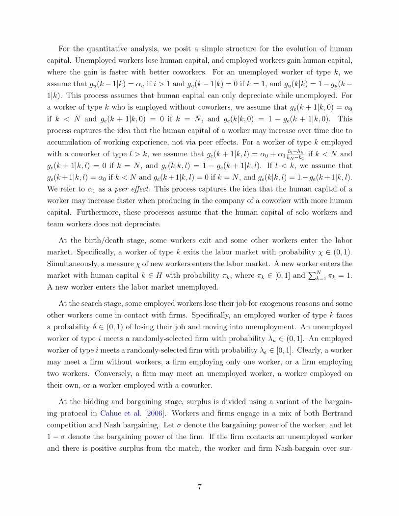
Time is discrete and continues forever. Each period is divided into five stages: learning,

births/deaths, search, bidding and bargaining, dismissal and production. Figure 1 illustrates

the timing of events within a period.

At the learning stage, the human capital of a worker of type k evolves according to a law of

motion that depends on the employment status of the worker as well as the human capital of

coworkers. Specifically, if the worker is unemployed, the worker’s human capital transitions

from k to k+ with probability gu(k+ | k), with gu(k+ | k) ∈ (0, 1) and∑

k+∈H gu(k+ | k) = 1.

If the worker is employed without a coworker, the worker’s human capital transitions from k

to k+ with probability ge(k+ | k), with ge(k+ | k) ∈ (0, 1) and∑

k+∈H ge(k+ | k) = 1. Finally,

if the worker is employed with a coworker of type l, the worker’s human capital transitions

from k to k+ with probability ge(k+ | k, l), with ge(k+ | k, l) ∈ (0, 1) and∑

k+∈H ge(k+ |k, l) = 1.

6

For the quantitative analysis, we posit a simple structure for the evolution of human

capital. Unemployed workers lose human capital, and employed workers gain human capital,

where the gain is faster with better coworkers. For an unemployed worker of type k, we

assume that gu(k− 1|k) = αu if i > 1 and gu(k− 1|k) = 0 if k = 1, and gu(k|k) = 1− gu(k−1|k). This process assumes that human capital can only depreciate while unemployed. For

a worker of type k who is employed without coworkers, we assume that ge(k + 1|k, 0) = α0

if k < N and ge(k + 1|k, 0) = 0 if k = N , and ge(k|k, 0) = 1 − ge(k + 1|k, 0). This

process captures the idea that the human capital of a worker may increase over time due to

accumulation of working experience, not via peer effects. For a worker of type k employed

with a coworker of type l > k, we assume that ge(k + 1|k, l) = α0 + α1hl−hkhN−h1

if k < N and

ge(k + 1|k, l) = 0 if k = N , and ge(k|k, l) = 1 − ge(k + 1|k, l). If l < k, we assume that

ge(k+ 1|k, l) = α0 if k < N and ge(k+ 1|k, l) = 0 if k = N , and ge(k|k, l) = 1− ge(k+ 1|k, l).We refer to α1 as a peer effect. This process captures the idea that the human capital of a

worker may increase faster when producing in the company of a coworker with more human

capital. Furthermore, these processes assume that the human capital of solo workers and

team workers does not depreciate.

At the birth/death stage, some workers exit and some other workers enter the labor

market. Specifically, a worker of type k exits the labor market with probability χ ∈ (0, 1).

Simultaneously, a measure χ of new workers enters the labor market. A new worker enters the

market with human capital k ∈ H with probability πk, where πk ∈ [0, 1] and∑N

k=1 πk = 1.

A new worker enters the labor market unemployed.

At the search stage, some employed workers lose their job for exogenous reasons and some

other workers come in contact with firms. Specifically, an employed worker of type k faces

a probability δ ∈ (0, 1) of losing their job and moving into unemployment. An unemployed

worker of type i meets a randomly-selected firm with probability λu ∈ (0, 1]. An employed

worker of type i meets a randomly-selected firm with probability λe ∈ [0, 1]. Clearly, a worker

may meet a firm without workers, a firm employing only one worker, or a firm employing

two workers. Conversely, a firm may meet an unemployed worker, a worker employed on

their own, or a worker employed with a coworker.

At the bidding and bargaining stage, surplus is divided using a variant of the bargain-

ing protocol in Cahuc et al. [2006]. Workers and firms engage in a mix of both Bertrand

competition and Nash bargaining. Let σ denote the bargaining power of the worker, and let

1 − σ denote the bargaining power of the firm. If the firm contacts an unemployed worker

and there is positive surplus from the match, the worker and firm Nash-bargain over sur-

7

plus. If the firm (henceforth, the poacher) contacts an employed worker, the poacher and

the current employer (henceforth, the incumbent) engage in Bertrand competition. If the

poacher’s value of hiring the employee is greater than the incumbent’s value of hiring the

employee, the worker moves to the poacher. The poacher and employee then Nash bargain

over surplus using the highest bid from Bertrand competition as the outside option of the

worker. Otherwise, the worker stays with the incumbent, and potentially renegotiates the

split of surplus. Note that if the poacher has two employees, it must dismiss one of them

if it succeeds in hiring the worker. During Bertrand competition, we assume that both the

incumbent and poacher observe each other’s fundamental states (i.e. how many workers each

employs and of what type), but not the offers. Therefore, bids can only be contingent on

the fundamental state and not on offers.

At the dismissal stage, the firm may separate from any of its employees. At the production

stage, firms and workers produce, workers receive their income and firms receive their profits.

Specifically, an employed worker of type k who does not have a coworker produces f(k, 0)

units of output and receives the income that is specified by the employment contract. An

employed worker of type k and a coworker of type l produce f(k, l) units of output. The

worker of type k receives the income that is specified by the employment contract. An

unemployed worker of type k receives an income of b(k), which the reader may interpret

as the value of home production, as an unemployment benefit, or as a combination of the

two. For the quantitative analysis, we assume that b(k) = φhk, with φ ∈ (0, 1). That is, the

income of an unemployed worker of type k is a fraction φ of the worker’s human capital.

We assume that employment contracts are complete. That is, an employment con-

tract specifies the worker’s employment probability contingent on the entire history of the

firm-worker match (e.g., the worker’s type, the worker’s contact with a poaching firm, the

coworker’s type, the coworker’s contact with another firm, and the firm’s contact with an-

other worker), the worker’s wage conditional on the history of the match, as well as the offers

that the firm makes to other workers. We assume that an employment contract must satisfy

the worker’s participation constraint. The constraint requires that, in all contingencies in

which the contract specifies the worker to be employed at the production stage, the life-

time utility of the contract to the worker must be greater than the value of unemployment.

Furthermore, in all contingencies in which the worker receives an offer from a poacher and

the contract specifies that the worker stays with the incumbent, the lifetime utility of the

contract to the worker must be greater than the expected value of the poacher’s offer. The

contract need not satisfy the firm’s participation constraint because the firm can commit to

8

participate.

3.2 Definition of Equilibrium

In order to define an equilibrium, we need to introduce some notation. We denote as U(k)

the lifetime utility of a worker of type k who is unemployed. We denote as Π0 the lifetime

profit of a firm that has no employees. We denote as V1(k) the sum of the lifetime profit

of a firm and the lifetime utility of a worker of type k who are matched together. We refer

to V1(k) as the joint value of a match between a firm and a worker of type k. We denote

as V2(k, l) the sum of the lifetime profit of a firm, the lifetime utility of a worker of type k,

and the lifetime utility of a worker of type l who are matched together. We refer to V2(k, l)

as the joint value of a match between a firm and a team of workers of type (k, l). The

value functions U(k), V1(k) and V2(k, l) are all evaluated at the beginning of the production

stage. We also find it useful to denote as V1(k) and as V2(k, l) the joint values of firm-worker

matches evaluated at the beginning of the dismissal stage.

We measure the distribution of workers across types and employment states at the be-

ginning of the search stage. We denote as uk the measure of workers of type k who are

unemployed at the beginning of the search stage. We denote as ek,0 the measure of workers

of type k who are employed without a coworker at the beginning of the search stage. Finally,

we denote as ek,l the measure of workers of type k who are employed with a coworker of type

l at the beginning of the search stage.

We restrict attention to equilibria with the following bidding and bargaining protocol.

Consider a poaching firm contacting an unemployed worker of type i. Let vP denote the

marginal value of the worker at the firm, where vP is equal to V1(k)−Π0 if the firm has no

employees, V2(k, i) − V1(k) if the firm has an employee of type k, max{V2(k, i), V2(i, l)} −V2(k, l) if the firm has two employees of type k and l. If vP > U(i), the firm and worker

Nash-bargain over surplus. If vP ≤ U(i), no match is formed.

Now, consider a firm contacting a worker of type i who is already employed. The marginal

value of the worker at the poaching firm is vP . Let vI denote the marginal value of the worker

at the incumbent, where vI is equal to V1(i) − Π0 if the worker is the only employee of the

incumbent and V2(i, j)− V1(j) if the incumbent also employs a worker of type j. There are

three cases. If vP > vI , the worker moves the poaching firm, and they Nash-bargain over the

division of surplus. The worker’s outside option is vI which is the most the incumbent firm is

9

willing to bid for the worker under Bertrand competition. Therefore, Nash bargaining yields

a value to the worker of vI +σ[vP − vI ]. If vP = vI , the poacher and the incumbent both bid

vI and the worker stays with the incumbent. If vP < vI , the poacher bids vP , the incumbent

offers a continuation value greater than vP , and the worker stays with the incumbent.

At the dismissal stage, the firm decides which workers to dismiss. Consider the case of a

firm with one type k employee. If the firm retains the employee, the joint continuation value

is V1(k). If the firm dismisses the employee, the continuation value to the firm is Π0 and the

continuation value to the worker is U(k). Therefore, the joint value V1(k) of a firm and an

employee of type k at the beginning of the dismissal stage is such that

V1(k) = max{V1(k),Π0 + U(k)}. (1)

Consider a firm with two employees, one of type k and one of type l. If the firm retains

both employees, the joint continuation value is V2(k, l). If the firm retains the k employee

and dismisses the l employee, the joint continuation value of the firm and the k employee is

V1(k) and the continuation value of the l employee is U(l). Similarly, if the firm retains the

l employee and dismisses the k employee, the joint continuation value to the firm and the l

employee is V1(l) and the continuation value of the k employee is U(k). Finally, if the firm

dismisses both employees, the continuation value of the firm is Π0, the continuation value

of the k worker is U(k) and the continuation value of the l worker is U(l). The joint value

V2(k, l) of a firm, an employee of type k and an employee of type l at the beginning of the

dismissal stage is such that

V2(k, l) = max{V2(k, l), V1(k) + U(l), V1(l) + U(k),Π0 + U(k) + U(l)}. (2)

The value Π0 of a firm without employees at the beginning of the production stage is

such that

Π0 =f(0, 0) + β[ N∑i=1

λuuiF

(1− σ) max{V1(i)− U(i)− Π0, 0}

+N∑i=1

N∑j=1

λeei,jF

(1− σ) max{V1(i)− [V2(i, j)− V1(j)]− Π0, 0}+ Π0

].

(3)

The flow profit of the firm is 0. In the next period, the firm contacts an unemployed worker

10

of type i with probability λuui/F . If there is positive surplus from the match, the firm hires

the worker and the firm’s continuation profit is a share (1− σ) of surplus, V1(i)−U(i)−Π0.

With probability λeei,0/F , the firm contacts a worker of type i who is currently employed

without a coworker. In this case, the incumbent keeps the worker since the employee has the

same marginal product at both the incumbent and poaching firm. Finally, with probability

λeei,j/F , the firm contacts a worker of type i who is employed with a worker of type j.

Suppose the worker’s marginal product at the poaching firm, V1(i) − Π0, is greater than

the worker’s marginal product at the incumbent, V2(i, j) − V1(j). Then through Bertrand

competition, the worker’s outside option is their marginal product at the incumbent firm,

V2(i, j)−V1(j). The firm hires the worker and they Nash-bargain over the division of surplus.

The firm’s continuation profit is a share (1−σ) of the surplus, V2(k+, i)−(V1(i)−Π0)−V1(k+).

If the worker’s marginal product is smaller at the poaching firm, then the poacher does not

hire the worker.

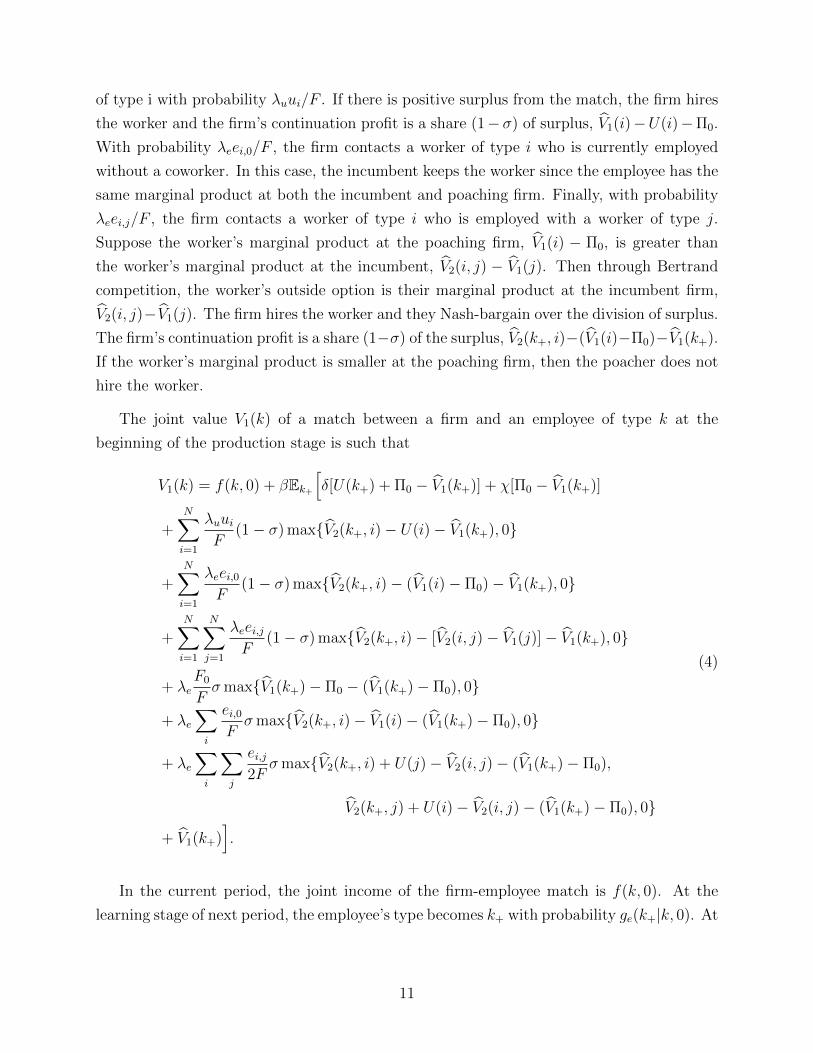
The joint value V1(k) of a match between a firm and an employee of type k at the

beginning of the production stage is such that

V1(k) = f(k, 0) + βEk+

[δ[U(k+) + Π0 − V1(k+)] + χ[Π0 − V1(k+)]

+N∑i=1

λuuiF

(1− σ) max{V2(k+, i)− U(i)− V1(k+), 0}

+N∑i=1

λeei,0F

(1− σ) max{V2(k+, i)− (V1(i)− Π0)− V1(k+), 0}

+N∑i=1

N∑j=1

λeei,jF

(1− σ) max{V2(k+, i)− [V2(i, j)− V1(j)]− V1(k+), 0}

+ λeF0

Fσmax{V1(k+)− Π0 − (V1(k+)− Π0), 0}

+ λe∑i

ei,0Fσmax{V2(k+, i)− V1(i)− (V1(k+)− Π0), 0}

+ λe∑i

∑j

ei,j2F

σmax{V2(k+, i) + U(j)− V2(i, j)− (V1(k+)− Π0),

V2(k+, j) + U(i)− V2(i, j)− (V1(k+)− Π0), 0}

+ V1(k+)].

(4)

In the current period, the joint income of the firm-employee match is f(k, 0). At the

learning stage of next period, the employee’s type becomes k+ with probability ge(k+|k, 0). At

11

the search stage of next period, the firm and the employee separate for exogenous reasons with

probability δ. In this case, the continuation value of the match is U(k+)+Π0. Likewise, with

probability χ, the worker dies. With probability λuui/F , the firm contacts an unemployed

worker of type i. In this case, the joint value of matching is V2(k+, i), the worker’s outside

option is U(i), and the firm’s outside option is V1(k). Thus, the surplus of the match is

V2(k+, i)−U(i)− V1(k+). If positive, the firm obtains a share (1− σ) of the surplus and the

worker is hired out of unemployment. With probability λeei,0/F , the firm contacts a worker

of type i who is employed without a coworker. In this case, the joint value of matching is

V2(k+, i), the outside option of the worker is (V1(i)−Π0), and the outside option of the firm

is Π0. Therefore, the surplus of the match is V2(k+, i) − (V1(i) − Π0) − V1(k+), and if its

positive the firm adds the type i worker to form a team. Lastly, with probability λeei,j/F ,

the firm contacts a worker of type i who is employed with a coworker of type j. In this case,

the joint value of matching is V2(k+, i), the outside option of the worker is V2(i, j) − V1(j),

and the outside option of the firm is Π0. If surplus is positive, the firm poaches i and forms

a team.

At the search stage, the employee may come into contact with a poacher. The employee

contacts a poacher without workers with probability λeF0/F , a poacher with a worker of

type i with probability λeei,0/F , and a poacher with a team of workers of type (i, j) with

probability λeei,j/(2F ). When the employee comes into contact with a poacher, the continu-

ation value of the match is unuchanged if the marginal value of the employee is higher at the

incumbent than at the poacher. If the marginal value of the employee is higher at the poacher

than at the incumbent, the match dissolves and the employee is hired by the poacher. When

the worker is poached, the outside option of the worker is their current marginal product,

(V1(k+) − Π0). The marginal product of the worker at the poacher is V1(k+) − Π0 at the

poacher with zero employees, V2(k+, i)− V1(i) at the poacher with one type i employee, and

max{V2(k+, i)+U(j)− V2(i, j), V2(k+, j)+U(i)− V2(i, j)} at the poacher with an (i, j) team.

The worker and poacher then Nash-bargain. Thus, the joint worker-firm team capture σ,

the worker’s share, of the surplus generated from the move.

The joint value V2(k, l) of a match between a firm, an employee of type k and an employee

of type l at the beginning of the production stage is such that

12

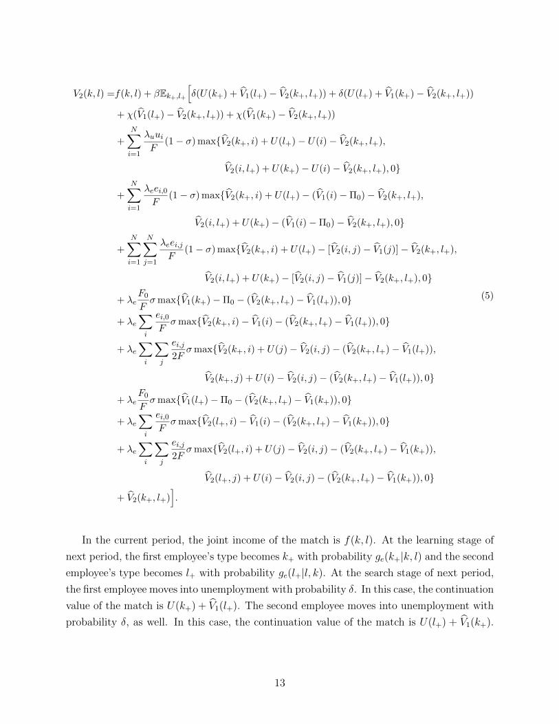
V2(k, l) =f(k, l) + βEk+,l+

[δ(U(k+) + V1(l+)− V2(k+, l+)) + δ(U(l+) + V1(k+)− V2(k+, l+))

+ χ(V1(l+)− V2(k+, l+)) + χ(V1(k+)− V2(k+, l+))

+

N∑i=1

λuuiF

(1− σ) max{V2(k+, i) + U(l+)− U(i)− V2(k+, l+),

V2(i, l+) + U(k+)− U(i)− V2(k+, l+), 0}

+N∑i=1

λeei,0F

(1− σ) max{V2(k+, i) + U(l+)− (V1(i)−Π0)− V2(k+, l+),

V2(i, l+) + U(k+)− (V1(i)−Π0)− V2(k+, l+), 0}

+N∑i=1

N∑j=1

λeei,jF

(1− σ) max{V2(k+, i) + U(l+)− [V2(i, j)− V1(j)]− V2(k+, l+),

V2(i, l+) + U(k+)− [V2(i, j)− V1(j)]− V2(k+, l+), 0}

+ λeF0

Fσmax{V1(k+)−Π0 − (V2(k+, l+)− V1(l+)), 0}

+ λe∑i

ei,0Fσmax{V2(k+, i)− V1(i)− (V2(k+, l+)− V1(l+)), 0}

+ λe∑i

∑j

ei,j2F

σmax{V2(k+, i) + U(j)− V2(i, j)− (V2(k+, l+)− V1(l+)),

V2(k+, j) + U(i)− V2(i, j)− (V2(k+, l+)− V1(l+)), 0}

+ λeF0

Fσmax{V1(l+)−Π0 − (V2(k+, l+)− V1(k+)), 0}

+ λe∑i

ei,0Fσmax{V2(l+, i)− V1(i)− (V2(k+, l+)− V1(k+)), 0}

+ λe∑i

∑j

ei,j2F

σmax{V2(l+, i) + U(j)− V2(i, j)− (V2(k+, l+)− V1(k+)),

V2(l+, j) + U(i)− V2(i, j)− (V2(k+, l+)− V1(k+)), 0}

+ V2(k+, l+)].

(5)

In the current period, the joint income of the match is f(k, l). At the learning stage of

next period, the first employee’s type becomes k+ with probability ge(k+|k, l) and the second

employee’s type becomes l+ with probability ge(l+|l, k). At the search stage of next period,

the first employee moves into unemployment with probability δ. In this case, the continuation

value of the match is U(k+) + V1(l+). The second employee moves into unemployment with

probability δ, as well. In this case, the continuation value of the match is U(l+) + V1(k+).

13

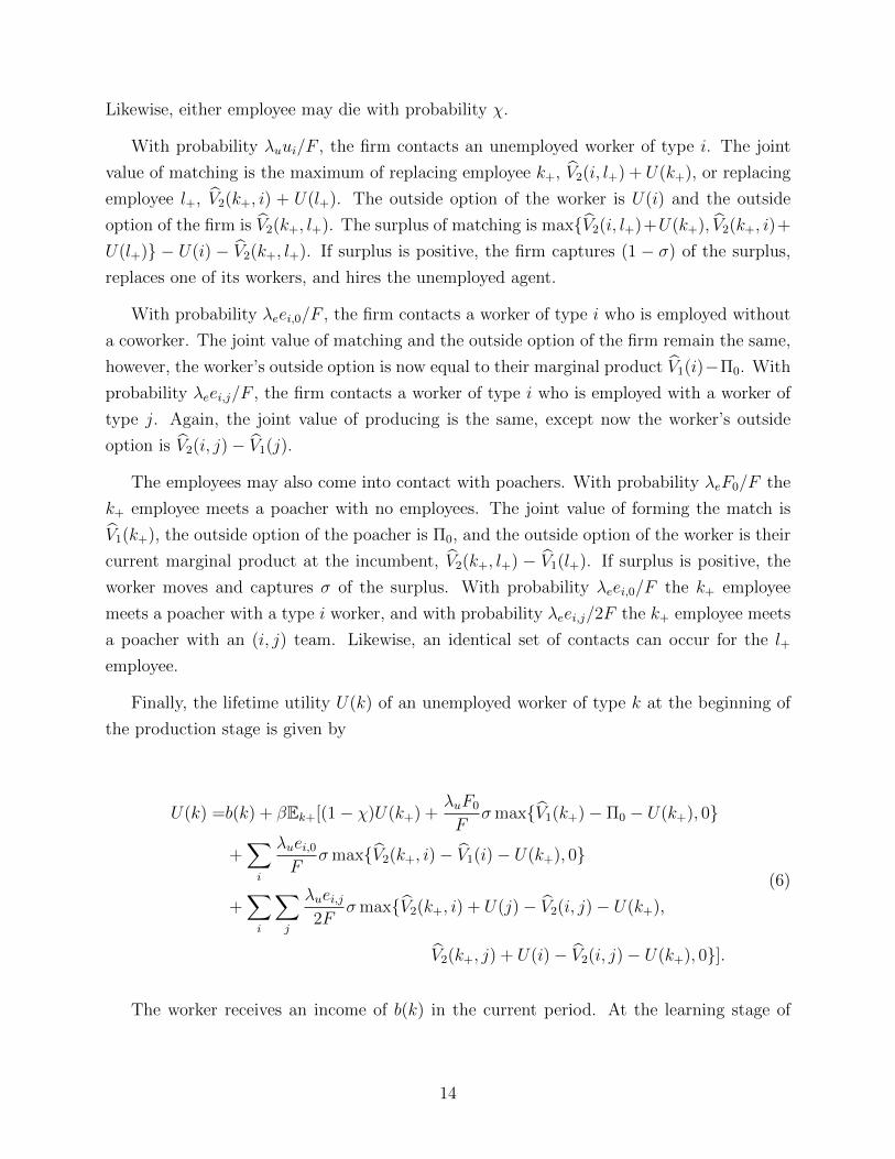
Likewise, either employee may die with probability χ.

With probability λuui/F , the firm contacts an unemployed worker of type i. The joint

value of matching is the maximum of replacing employee k+, V2(i, l+) + U(k+), or replacing

employee l+, V2(k+, i) + U(l+). The outside option of the worker is U(i) and the outside

option of the firm is V2(k+, l+). The surplus of matching is max{V2(i, l+)+U(k+), V2(k+, i)+

U(l+)} − U(i) − V2(k+, l+). If surplus is positive, the firm captures (1 − σ) of the surplus,

replaces one of its workers, and hires the unemployed agent.

With probability λeei,0/F , the firm contacts a worker of type i who is employed without

a coworker. The joint value of matching and the outside option of the firm remain the same,

however, the worker’s outside option is now equal to their marginal product V1(i)−Π0. With

probability λeei,j/F , the firm contacts a worker of type i who is employed with a worker of

type j. Again, the joint value of producing is the same, except now the worker’s outside

option is V2(i, j)− V1(j).

The employees may also come into contact with poachers. With probability λeF0/F the

k+ employee meets a poacher with no employees. The joint value of forming the match is

V1(k+), the outside option of the poacher is Π0, and the outside option of the worker is their

current marginal product at the incumbent, V2(k+, l+) − V1(l+). If surplus is positive, the

worker moves and captures σ of the surplus. With probability λeei,0/F the k+ employee

meets a poacher with a type i worker, and with probability λeei,j/2F the k+ employee meets

a poacher with an (i, j) team. Likewise, an identical set of contacts can occur for the l+

employee.

Finally, the lifetime utility U(k) of an unemployed worker of type k at the beginning of

the production stage is given by

U(k) =b(k) + βEk+[(1− χ)U(k+) +λuF0

Fσmax{V1(k+)− Π0 − U(k+), 0}

+∑i

λuei,0F

σmax{V2(k+, i)− V1(i)− U(k+), 0}

+∑i

∑j

λuei,j2F

σmax{V2(k+, i) + U(j)− V2(i, j)− U(k+),

V2(k+, j) + U(i)− V2(i, j)− U(k+), 0}].

(6)

The worker receives an income of b(k) in the current period. At the learning stage of

14

next period, the worker’s type becomes k+ with probability gu(k+|k). With probability χ the

employee dies. At the search stage, the worker does not contact any firm with probability

1 − λu. In this case, the worker’s continuation value is U(k+). With probability λuF0/F ,

the unemployed worker contacts a firm with zero employees, with probability λuei,0/F the

unemployed worker contacts a firm with a type i employee, and with λuei,j/2F the unem-

ployed worker contacts a firm with an (i, j) team. In each case, the worker obtains a share

σ of the surplus if a match is consummated.

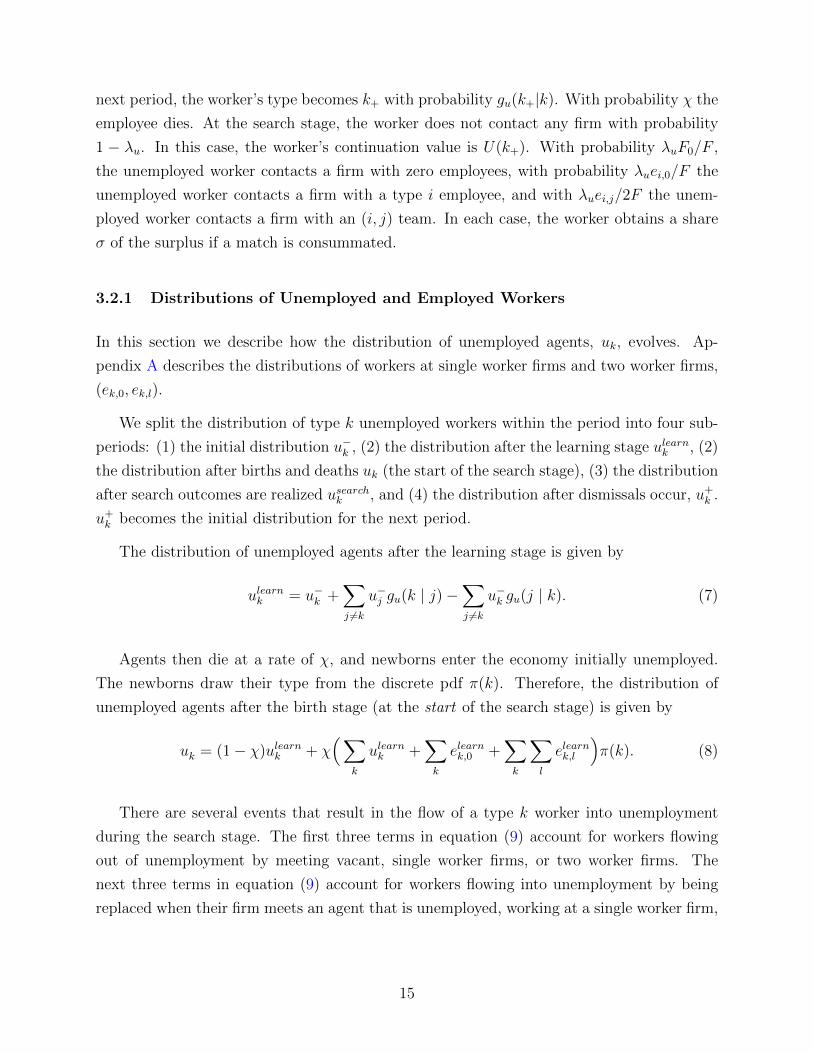
3.2.1 Distributions of Unemployed and Employed Workers

In this section we describe how the distribution of unemployed agents, uk, evolves. Ap-

pendix A describes the distributions of workers at single worker firms and two worker firms,

(ek,0, ek,l).

We split the distribution of type k unemployed workers within the period into four sub-

periods: (1) the initial distribution u−k , (2) the distribution after the learning stage ulearnk , (2)

the distribution after births and deaths uk (the start of the search stage), (3) the distribution

after search outcomes are realized usearchk , and (4) the distribution after dismissals occur, u+k .

u+k becomes the initial distribution for the next period.

The distribution of unemployed agents after the learning stage is given by

ulearnk = u−k +∑j 6=k

u−j gu(k | j)−∑j 6=k

u−k gu(j | k). (7)

Agents then die at a rate of χ, and newborns enter the economy initially unemployed.

The newborns draw their type from the discrete pdf π(k). Therefore, the distribution of

unemployed agents after the birth stage (at the start of the search stage) is given by

uk = (1− χ)ulearnk + χ(∑

k

ulearnk +∑k

elearnk,0 +∑k

∑l

elearnk,l

)π(k). (8)

There are several events that result in the flow of a type k worker into unemployment

during the search stage. The first three terms in equation (9) account for workers flowing

out of unemployment by meeting vacant, single worker firms, or two worker firms. The

next three terms in equation (9) account for workers flowing into unemployment by being

replaced when their firm meets an agent that is unemployed, working at a single worker firm,

15

or working at a two worker firm. The last line of equation (9) accounts for exogenous layoffs.

usearchk = uk − ukλuF0

FI(V1(k)−Π0 − U(k) > 0)

− uk∑i

λuei,0

FI(V2(k, i)− U(k)− V1(i) > 0)

− uk∑i

∑j

(λuei,j

2FI(max{V2(k, j) + U(i)− U(k)− V2(i, j), V2(i, k) + U(j)− U(k)− V2(i, j)} > 0))

+∑i

ek,lλuuiF

I(max{V2(k, i) + U(l)− U(i)− V2(k, l), V2(i, l) + U(k)− U(i)− V2(k, l)} > 0)

× I(V2(i, l) + U(k)− U(i)− V2(k, l) > V2(k, i) + U(l)− U(i)− V2(k, l))

+∑i

ek,lλeei,0

FI(max{V2(k, i) + U(l)− (V1(i)−Π0)− V2(k, l), V2(i, l) + U(k)− (V1(i)−Π0)− V2(k, l)} > 0)

× I(V2(i, l) + U(k)− (V1(i)−Π0)− V2(k, l) > V2(k, i) + U(l)− (V1(i)−Π0)− V2(k, l))

+∑i

∑j

ek,lλeei,j

FI(max{V2(k, i) + U(l)− (V2(i, j)− V1(j))− V2(k, l), V2(i, l) + U(k)− (V2(i, j)− V1(j))− V2(k, l)} > 0)

× I(V2(i, l) + U(k)− (V2(i, j)− V1(j))− V2(k, l) > V2(k, i) + U(l)− (V2(i, j)− V1(j))− V2(k, l))

+ δ(ek,0 +

∑i

ek,i

)(9)

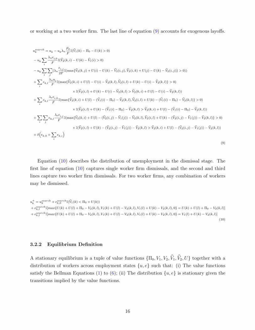
Equation (10) describes the distribution of unemployment in the dismissal stage. The

first line of equation (10) captures single worker firm dismissals, and the second and third

lines capture two worker firm dismissals. For two worker firms, any combination of workers

may be dismissed.

u+k = usearchk + esearchk,0 I(V1(k) < Π0 + U(k))

+ esearchk,l I[max{U(k) + U(l) + Π0 − V2(k, l), V1(k) + U(l)− V2(k, l), V1(l) + U(k)− V2(k, l), 0} = U(k) + U(l) + Π0 − V2(k, l)]

+ esearchk,l I[max{U(k) + U(l) + Π0 − V2(k, l), V1(k) + U(l)− V2(k, l), V1(l) + U(k)− V2(k, l), 0} = V1(l) + U(k)− V2(k, l)]

(10)

3.2.2 Equilibrium Definition

A stationary equilibrium is a tuple of value functions {Π0, V1, V2, V1, V2, U} together with a

distribution of workers across employment states {u, e} such that: (i) The value functions

satisfy the Bellman Equations (1) to (6); (ii) The distribution {u, e} is stationary given the

transitions implied by the value functions.

16

3.3 Wage determination

We assume promised values are delivered using a fixed wage. The wage changes only if the

worker receives an outside offer, a coworker is added, a coworker is lost, or the promised

value of the worker exceeds the worker’s marginal product.

Let vW denote the current promised value to the worker. There are three cases to consider.

Suppose the worker contacts a poaching firm where vP < vW . Then the contact does not

generate a wage change. Suppose the worker meets a poaching firm where vW < vP < vI .

The worker stays with the incumbent and triggers Bertrand competition. The worker receives

a new constant wage which delivers a promised value equal to vP . Suppose the worker meets

a poaching firm where vI < vP . The worker switches employers. The worker’s outside option

is to trigger Bertrand competition which yields, vI . The worker then Nash-bargains over the

remaining surplus generated with the poaching firm. The worker receives a new constant

wage which delivers the promised value of vI + σ[vP − vI ].

To facilitate exposition, we introduce some additional notation. Let the value of obtaining

an outside offer to an employee from a poacher with marginal product vP be

A(vP , vI) = min{vP , vI + σmax{vP − vI , 0}}.

17

The value function of a type k worker being paid w is given by,

W1(k,w) = w + βEk+[δU(k+)

+ λeF0

Fmax{min{W1(k+, w), V1(k+)−Π0}, U(k+), A

(V1(k+)−Π0, V1(k+)−Π0

)}

+∑i

λeei,0F

max{

min{W1(k+, w), V1(k+)−Π0}, U(k+), A(V2(k+, i)− V1(i), V1(k+)−Π0

)}+∑i

∑j

λeei,j2F

max{

min{W1(k+, w), V1(k+)−Π0}, U(k+),

A(

max{V2(k+, i) + U(j)− V2(i, j), V2(k+, j) + U(i)− V2(i, j)}, V1(k+)−Π0

)}+

N∑i=1

λuuiF

I(V2(k+, i)− U(i) > V1(k+)) max{min{W2(k+, i, w), V2(k+, i)− V1(i)}, U(k+)}

+

N∑i=1

λeei,0F

I(V2(k+, i)− (V1(i)−Π0) > V1(k+)) max{min{W2(k+, i, w), V2(k+, i)− V1(i)}, U(k+)}

+N∑i=1

N∑j=1

λeei,jF

I(V2(k+, i)− [V2(i, j)− V1(j)] > V1(k+)) max{min{W2(k+, i, w), V2(k+, i)− V1(i)}, U(k+)}]

+ (1− δ − λe − χ−H(k)) max{min{W1(k+, w), V1(k+)−Π0}, U(k+)}

With probability H(k), a coworker is added:

H(k) =

N∑i=1

λuuiF

I(V2(k+, i)− U(i) > V1(k+))

+

N∑i=1

λeei,0F

I(V2(k+, i)− (V1(i)−Π0) > V1(k+))

+

N∑i=1

N∑j=1

λeei,jF

I(V2(k+, i)− [V2(i, j)− V1(j)] > V1(k+))

The value function of a type k worker being paid w while matched with a type l coworker

is given by,

18

W2(k, l, w) = w + βEk+,l+ [(δ +R(k+, l+))U(k+) + P (k+, l+) max{min{W1(k+, w), V1(k+)−Π0}, U(k+)}

+ λeF0

Fmax

{min{W2(k+, l+, w), V2(k+, l+)− V1(l+)}, U(k+), A

(V1(k+)−Π0, V2(k+, l+)− V1(l+)

)}+∑i

λeei,0F

max

{min{W2(k+, l+, w), V2(k+, l+)− V1(l+)}, U(k+), A

(V2(k+, i)− V1(i), V2(k+, l+)− V1(l+)

)}

+∑i

∑j

λeei,j2F

max

{min{W2(k+, l+, w), V2(k+, l+)− V1(l+)}, U(k+),

A(

max{V2(k+, i) + U(j)− V2(i, j), V2(k+, j) + U(i)− V2(i, j)}, V2(k+, l+)− V1(l+))}

+

N∑i=1

λuuiF

I(V2(k+, i) + U(l+)− U(i) > V2(k+, l+)) max{min{W2(k+, i, w), V2(k+, i)− V1(i)}, U(k+)}

+

N∑i=1

λeei,0F

I(V2(k+, i) + U(l+)− (V1(i)−Π0) > V2(k+, l+)) max{min{W2(k+, i, w), V2(k+, i)− V1(i)}, U(k+)}

+

N∑i=1

N∑j=1

λeei,jF

I(V2(k+, i) + U(l+)− [V2(i, j)− V1(j)] > V2(k+, l+)) max{min{W2(k+, i, w), V2(k+, i)− V1(i)}, U(k+)}]

+ (1− δ − λe − χ−R(k+, l+)− P (k+, l+)−Q(k+, l+)) max{min{W2(k+, l+, w), V2(k+, l+)− V1(l+)}, U(k+)}

The probability a type k worker is replaced in a (k, l) team is given by,

R(k, l) =∑i

λuuiF

I(max{V2(k, i) + U(l)− U(i)− V2(k, l), V2(i, l) + U(k)− U(i)− V2(k, l)} > 0)

× I(V2(i, l) + U(k)− U(i)− V2(k, l) > V2(k, i) + U(l)− U(i)− V2(k, l))

+∑i

λeei,0F

I(max{V2(k, i) + U(l)− (V1(i)−Π0)− V2(k, l), V2(i, l) + U(k)− (V1(i)−Π0)− V2(k, l)} > 0)

× I(V2(i, l) + U(k)− (V1(i)−Π0)− V2(k, l) > V2(k, i) + U(l)− (V1(i)−Π0)− V2(k, l))

+∑i

∑j

λeei,jF

I(max{V2(k, i) + U(l)− (V2(i, j)− V1(j))− V2(k, l), V2(i, l) + U(k)− (V2(i, j)− V1(j))− V2(k, l)} > 0)

× I(V2(i, l) + U(k)− (V2(i, j)− V1(j))− V2(k, l) > V2(k, i) + U(l)− (V2(i, j)− V1(j))− V2(k, l))

19

With probability P (k, l) the type l coworker leaves the firm:

P (k, l) = λeF0

FI(V1(l)− (V2(k, l)− V1(k))−Π0 > 0) +

∑i

λeei,0F

I(V2(l, i)− (V2(k, l)− V1(k))− V1(i) > 0)

+∑i

∑j

λeei,j2F

I(max{V2(l, i) + U(j)− (V2(k, l)− V1(k))− V2(i, j),

V2(l, j) + U(i)− (V2(k, l)− V1(k))− V2(i, j)} > 0)

With probability Q(k, l) the type l coworker is replaced:

Q(k, l) =

N∑i=1

λuuiF

I(V2(k, i) + U(l)− U(i) > V2(k, l)) +

N∑i=1

λeei,0F

I(V2(k, i) + U(l+)− (V1(i)−Π0) > V2(k, l))

+

N∑i=1

N∑j=1

λeei,jF

I(V2(k, i) + U(l)− [V2(i, j)− V1(j)] > V2(k, l))

20

4 Calibration

The model is calibrated so that one period is one month. The death rate, χ, is .003% per

month, corresponding to a 30 year working life. The discount factor is set to β = .9816,

which corresponds to a discount rate of 25% per annum.3 The production function is given

by f(k, l) = (h1ρ

k +h1ρ

l )ρ. ρ controls the degree of complementarity between types. We discuss

the estimation of ρ in more detail below.

We assume there are N = 7 types. We assume productive abilities are evenly spaced

between h1 and h7. We normalize h1 to equal 1 and we estimate h7 to match the p90/p10

wage ratio in the pooled 2000-2016 Current Population Survey Merged Outgoing Rotation

Groups (henceforth, the CPS).

The bargaining weight of the unemployed workers, σ, is estimated to match the ratio of

the average wage of job finders to the average wage of employed individuals in the CPS. We

estimate home production φ to match the 16% decline in consumption after 6 months of

unemployment reported by Browning and Crossley [2001].

For newborns, we assume that the type-distribution of newborns is a discrete truncated

normal distribution over the productive abilities, {h1, . . . , h7}, with mean mnew and variance

vnew. We parameterize the mean and variance parameters to target (i) the mean wage of

22-24 year old individuals to the average wage of employed individuals in the CPS, and (ii)

the p90 to p10 wage ratio for this subgroup in the CPS.

We normalize the measure of firms, F, to a unit mass, and the parameters that govern

the unemployed job contact rate, the employed job contact rate, and the job destruction

rate, {λu, λe, δ}, are set to target the job finding rate, the job-to-job transition rate, and the

unemployment rate as measured in the CPS.

We estimate the rate of human capital depreciation among the unemployed, αu, to match

the negative relationship between the job finding hazard and unemployment in the CPS. We

estimate the rate of human capital appreciation for solo workers, α0, to match the lifecycle

profile of wages in the CPS.

The production complementarity parameter, ρ, and the learning parameter for teams,

α1, are estimated jointly to match three sets of moments: (i) job flows as function of the

coworker-worker wage gap, (ii) the relationship between future wages and prior coworker

3This large discount rate allows us to avoid negative wages.

21

wage for EUE transitioners, and (iii) the share of wage variance that is between firms.

The first set of moments exploit the fact that learning has unique predictions about job-

to-job flows and the relative wage of a worker and their coworker. Through the lens of the

model, the worker’s wage is a noisy proxy of an individual’s type and the coworker’s wage

is a noisy proxy of the coworker’s type. With strong production complementarity and no

learning, the further a worker’s wage is from their coworker’s wage, the more likely they are

to switch employers in search of a better match. With strong learning and no production

complementarity, the further a worker’s wage is from their coworker’s wage, the less likely

they are to switch employers because they are either learning or teaching their coworker.

The second set of moments we use to disentangle learning and sorting are based on

the correlation between an individual’s wage and their old coworkers’ wages. To parse out

sticky-wages, built-up rents, and other forces which drive a wedge between a worker’s type

and their true productivity, we focus on individuals who separate, experience a spell of

unemployment, and then find a new job. We refer to this as an ‘EUE’ transition. As

sorting improves, coworker wages become a stronger predictor of the worker’s type, and thus

coworker wages become better predictors of future individual wages. As learning improves,

coworkers also become a stronger determinanet of future individual wages. The fact that

both learning and sorting move this moment in the same direction allows us to pin down the

level of sorting and learning.

And our last moment is the share of wage variance that is between firms. Since there

are multiple workers at a firm in our model, our framework has a concept of within-firm and

between-firm wage variance. As production complementarities increase, between-firm wage

variance grows relative to within-firm wage variance. As learning becomes more important,

within-firm wage variance share grows. Let V (wi,t) denote total wage variance, let wi,t denote

individual i’s wage at date t, let wfi,t denote the average wage of firm f where individual i

works at time t, and let wt denote the economy wide average wage at date t. We decompose

wage variance as follows,

V (wi,t) =1

N

N∑i=1

(wi,t − wfi,t)2

︸ ︷︷ ︸within

+1

N

N∑i=1

(wfi,t − wt)2

︸ ︷︷ ︸between

According to Spletzer [2014], 50.3% of cross-sectional earnings variance is across firms in the

LEHD.

22

We describe our estimation of the job-to-job flow moments in Section 4.1 and the worker-

coworker wage moments in 4.2.

4.1 Job mobility and the coworker-worker wage gap

To estimate job mobility as a function of coworker and worker wages, we use a 10% random

sample from the Longitudinal Employer-Household Dynamics database between 2001 and

2008.4 We restrict our sample to prime-age (24-65) males at single-unit firms with between

2 and 250 employees. We also require individuals in our sample to be employed throughout

the previous year at the same primary employer.5 We define a job-to-job transition from year

t to t + 1 if the individual switches primary employers without a spell of non-employment

(earning $1k or less in a quarter).

Let i index individuals and let t index years. Let JJi,t+1 be a dummy for a job-to-job

transition between t and t+1. Let wi,t denote log real annual earnings of individual i (which

we will refer to as an individual’s wage in the LEHD) at his/her primary employer in year

t.6 Let w−i,t denote the log real average annual wage of the coworkers of an individual at

his/her primary employer in year t, excluding individual i. We refer to w−i,t − wi,t) as the

‘wage gap.’ We estimate the following specifications separately for those above the average

wage at their firm (wi,t > w−i,t) and those below (wi,t < w−i,t):

JJi,t+1 = β0 + γt + β1wi,t + β2(w−i,t − wi,t) + ΓXi,t + εi,t (11)

Our regression controls, Xi,t, include firm size, state dummies, 1-digit sic dummies, race

dummies, education dummies, quadratics in age and tenure, as well as year fixed effects. All

standard errors are clustered at the SEIN level.

Table 1 provides summary statistics in our main sample.7 The annual job-to-job transi-

tion rate is 3.6% per annum. The average age of an individual in our sample is 41, and they

4The LEHD database is a matched employer-employee dataset that covers 95% of U.S. private sectorjobs. The LEHD includes data on earnings, worker demographic characteristics, firm identifiers, and firmcharacteristics. Our data covers 2001 through 2008 for 11 states: California, Illinois, Indiana, Maryland,Nevada, New Jersey, Oregon, Rhode Island, Texas, Virginia, and Washington.

5We count individuals as employed if they earn $1k or more from an employer in a given quarter. Wecount individuals as non-employed if they earn less than $1k in a given quarter. The primary employer isthe employer that pays the worker the most.

6All variables which are not bounded above are winsorized at the 1% level. Nominal variables are deflatedusing the CPI.

7For disclosure purposes, we were required to round the sample size to the nearest thousand.

23

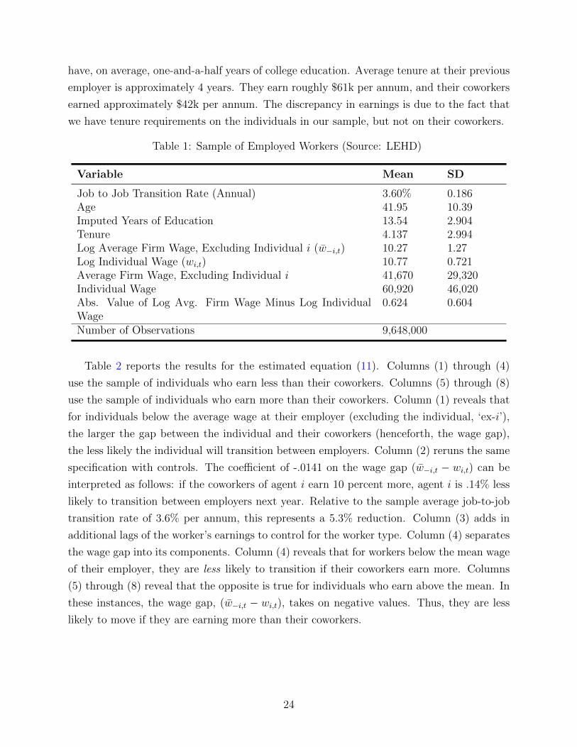
have, on average, one-and-a-half years of college education. Average tenure at their previous

employer is approximately 4 years. They earn roughly $61k per annum, and their coworkers

earned approximately $42k per annum. The discrepancy in earnings is due to the fact that

we have tenure requirements on the individuals in our sample, but not on their coworkers.

Table 1: Sample of Employed Workers (Source: LEHD)

Variable Mean SD

Job to Job Transition Rate (Annual) 3.60% 0.186Age 41.95 10.39Imputed Years of Education 13.54 2.904Tenure 4.137 2.994Log Average Firm Wage, Excluding Individual i (w−i,t) 10.27 1.27Log Individual Wage (wi,t) 10.77 0.721Average Firm Wage, Excluding Individual i 41,670 29,320Individual Wage 60,920 46,020Abs. Value of Log Avg. Firm Wage Minus Log IndividualWage

0.624 0.604

Number of Observations 9,648,000

Table 2 reports the results for the estimated equation (11). Columns (1) through (4)

use the sample of individuals who earn less than their coworkers. Columns (5) through (8)

use the sample of individuals who earn more than their coworkers. Column (1) reveals that

for individuals below the average wage at their employer (excluding the individual, ‘ex-i’),

the larger the gap between the individual and their coworkers (henceforth, the wage gap),

the less likely the individual will transition between employers. Column (2) reruns the same

specification with controls. The coefficient of -.0141 on the wage gap (w−i,t − wi,t) can be

interpreted as follows: if the coworkers of agent i earn 10 percent more, agent i is .14% less

likely to transition between employers next year. Relative to the sample average job-to-job

transition rate of 3.6% per annum, this represents a 5.3% reduction. Column (3) adds in

additional lags of the worker’s earnings to control for the worker type. Column (4) separates

the wage gap into its components. Column (4) reveals that for workers below the mean wage

of their employer, they are less likely to transition if their coworkers earn more. Columns

(5) through (8) reveal that the opposite is true for individuals who earn above the mean. In

these instances, the wage gap, (w−i,t − wi,t), takes on negative values. Thus, they are less

likely to move if they are earning more than their coworkers.

24

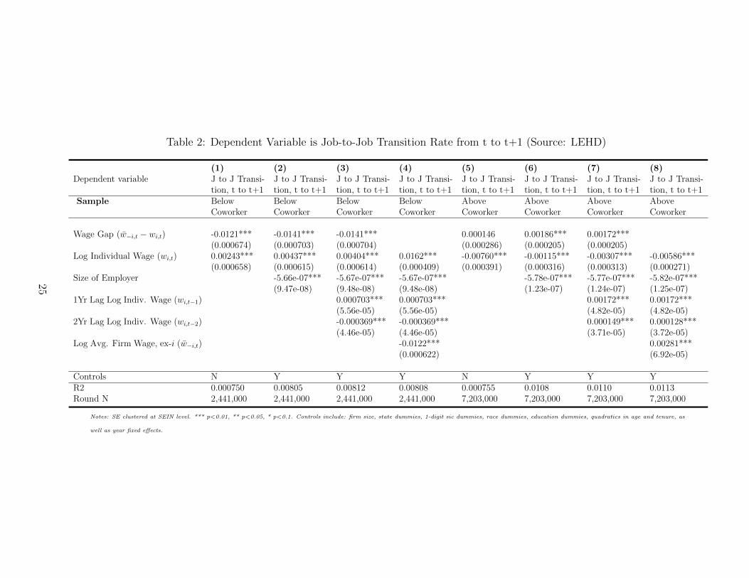
Table 2: Dependent Variable is Job-to-Job Transition Rate from t to t+1 (Source: LEHD)

(1) (2) (3) (4) (5) (6) (7) (8)Dependent variable J to J Transi-

tion, t to t+1J to J Transi-tion, t to t+1

J to J Transi-tion, t to t+1

J to J Transi-tion, t to t+1

J to J Transi-tion, t to t+1

J to J Transi-tion, t to t+1

J to J Transi-tion, t to t+1

J to J Transi-tion, t to t+1

Sample BelowCoworker

BelowCoworker

BelowCoworker

BelowCoworker

AboveCoworker

AboveCoworker

AboveCoworker

AboveCoworker

Wage Gap (w−i,t − wi,t) -0.0121*** -0.0141*** -0.0141*** 0.000146 0.00186*** 0.00172***(0.000674) (0.000703) (0.000704) (0.000286) (0.000205) (0.000205)

Log Individual Wage (wi,t) 0.00243*** 0.00437*** 0.00404*** 0.0162*** -0.00760*** -0.00115*** -0.00307*** -0.00586***(0.000658) (0.000615) (0.000614) (0.000409) (0.000391) (0.000316) (0.000313) (0.000271)

Size of Employer -5.66e-07*** -5.67e-07*** -5.67e-07*** -5.78e-07*** -5.77e-07*** -5.82e-07***(9.47e-08) (9.48e-08) (9.48e-08) (1.23e-07) (1.24e-07) (1.25e-07)

1Yr Lag Log Indiv. Wage (wi,t−1) 0.000703*** 0.000703*** 0.00172*** 0.00172***(5.56e-05) (5.56e-05) (4.82e-05) (4.82e-05)

2Yr Lag Log Indiv. Wage (wi,t−2) -0.000369*** -0.000369*** 0.000149*** 0.000128***(4.46e-05) (4.46e-05) (3.71e-05) (3.72e-05)

Log Avg. Firm Wage, ex-i (w−i,t) -0.0122*** 0.00281***(0.000622) (6.92e-05)

Controls N Y Y Y N Y Y YR2 0.000750 0.00805 0.00812 0.00808 0.000755 0.0108 0.0110 0.0113Round N 2,441,000 2,441,000 2,441,000 2,441,000 7,203,000 7,203,000 7,203,000 7,203,000

Notes: SE clustered at SEIN level. *** p<0.01, ** p<0.05, * p<0.1. Controls include: firm size, state dummies, 1-digit sic dummies, race dummies, education dummies, quadratics in age and tenure, as

well as year fixed effects.

25

4.2 Wages and past coworkers

We measure the correlation of future wages and past coworker wages by focusing on individ-

uals who transition between employers through a spell of unemployment (‘EUE’ transitions).

Through the lens of our model, this type of job transition parses out wage stickiness and

built-up rents, and so wages out of unemployment are a better proxy of the worker’s hu-

man capital. The relationship between prior coworker wages and future individual wages

reflect both sorting and learning. As sorting increases, coworker wages become a better

proxy of worker type and therefore become more correlated with future individual wages.

As learning increases, coworker wages become more correlated with future individual wages

via knowledge diffusion.

We identify EUE transitions in the data as those who have at least 1 year of tenure in year

t at their primary employer, spend at least one quarter non-employed in year t+1 (defined as

earning less than $1k in the quarter), and then obtain a job at a different primary employer

in year t+2. Let i index people who make an EUE transition and let t index years. The

dependent variable of interest is individual i’s log annual earnings in year t+2, wi,t+2. We

regress that on their own log wage prior to the unemployment spell, wi,t, as well as the log

real average annual wage of the coworkers, w−i,t. We estimate the following specifications:

wi,t+2 = β0 + γt + β1wi,t + β2w−i,t + ΓXi,t + εi,t (12)

Our regression controls, Xi,t, include firm size, state dummies, 1-digit sic dummies, race

dummies, education dummies, quadratics in age and tenure, as well as year fixed effects.

Table 3 provides summary statistics for our sample of EUE job transitioners prior to

their unemployment spell (date t). The average age of an individual in our sample is 38,

and they have, on average, one year of college education. Average tenure at their previous

employer is approximately 3 years. They earn roughly $39k per annum, and their coworkers

earn approximately $30k per annum. As before, the discrepancy in earnings is due to the

fact that we have a tenure requirement on the individuals in our sample, but not on their

coworkers.

Table 4 includes the results from estimating equation 12 for our sample of EUE transition-

ers. Columns (1) through (3) restrict the sample to those who earn less than their coworkers

at their previous firm in year t. Column (1) includes no controls. The point estimate im-

plies that across all workers who experienced an EUE transition between t and t+2, a 10%

26

Table 3: Summary Statistics of EUE Transitioners (Source: LEHD)

Variable Mean SD

Age 38.2 9.5Imputed Years of Education 13.0 2.9Tenure 2.9 2.3Log Average Firm Wage, Excluding Individual i (w−i,t) 10.0 0.8Log Individual Wage (wi,t) 10.4 0.7Average Firm Wage, Excluding Individual i 30,436 21,743Individual Wage 39,365 28,267Number of observations 55000

greater coworker wage prior to the unemployment spell is associated with a 1.34% greater

individual wage coming out of the unemployment spell. Column (2) includes controls, and

the point estimate implies that a 10% greater coworker wage prior to the unemployment

spell is associated with a 1.25% greater individual wage coming out of the unemployment

spell. Column (3) adds additional lags of the worker’s wage as a better proxy for the worker’s

type, and the point estimate does not change. Columns (4) through (6) restrict the sample

to those who earn more than their coworkers at their previous firm in year t, and we see a

much more muted relationship. The point estimates in Column (5) imply that a 10% greater

coworker wage prior to the unemployment spell is associated with a .16% greater individual

wage coming out of the unemployment spell.

What is consistent across all specifications is that prior firm size is negatively related to

future wages. We view this as suggestive evidence that our results are not being driven by

network effects.

27

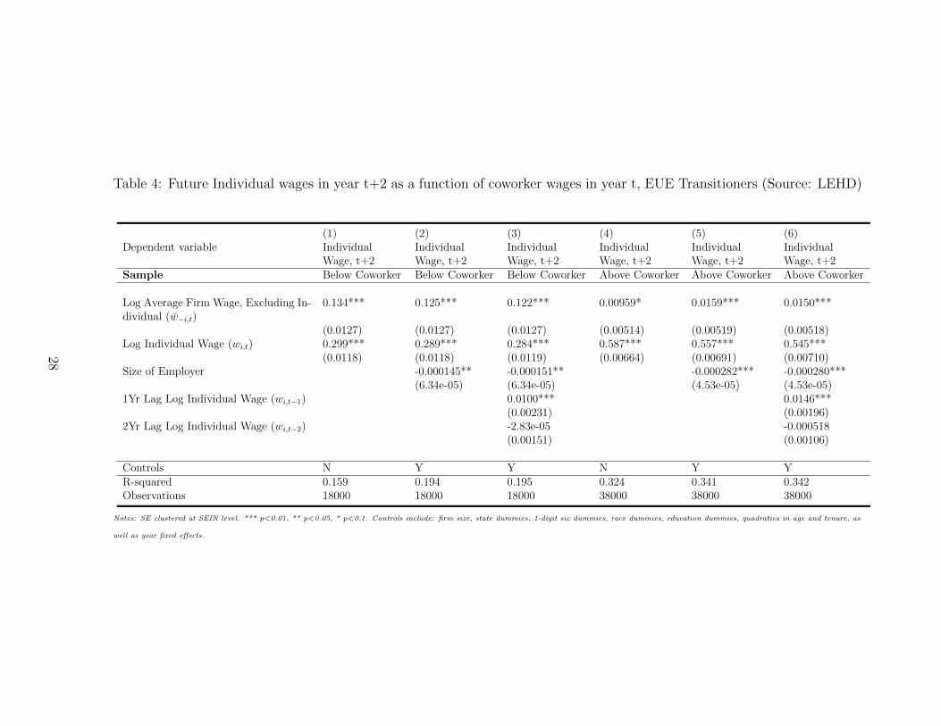
Table 4: Future Individual wages in year t+2 as a function of coworker wages in year t, EUE Transitioners (Source: LEHD)

(1) (2) (3) (4) (5) (6)Dependent variable Individual

Wage, t+2IndividualWage, t+2

IndividualWage, t+2

IndividualWage, t+2

IndividualWage, t+2

IndividualWage, t+2

Sample Below Coworker Below Coworker Below Coworker Above Coworker Above Coworker Above Coworker

Log Average Firm Wage, Excluding In-dividual (w−i,t)

0.134*** 0.125*** 0.122*** 0.00959* 0.0159*** 0.0150***

(0.0127) (0.0127) (0.0127) (0.00514) (0.00519) (0.00518)Log Individual Wage (wi,t) 0.299*** 0.289*** 0.284*** 0.587*** 0.557*** 0.545***

(0.0118) (0.0118) (0.0119) (0.00664) (0.00691) (0.00710)Size of Employer -0.000145** -0.000151** -0.000282*** -0.000280***

(6.34e-05) (6.34e-05) (4.53e-05) (4.53e-05)1Yr Lag Log Individual Wage (wi,t−1) 0.0100*** 0.0146***

(0.00231) (0.00196)2Yr Lag Log Individual Wage (wi,t−2) -2.83e-05 -0.000518

(0.00151) (0.00106)

Controls N Y Y N Y YR-squared 0.159 0.194 0.195 0.324 0.341 0.342Observations 18000 18000 18000 38000 38000 38000

Notes: SE clustered at SEIN level. *** p<0.01, ** p<0.05, * p<0.1. Controls include: firm size, state dummies, 1-digit sic dummies, race dummies, education dummies, quadratics in age and tenure, as

well as year fixed effects.

28

Appendix D includes additional robustness checks and reruns our specifications on Brazil-

ian data.8 We conduct several exercises: (i) we specify coworker wages within a firm and

2-digit occupation, (ii) we follow workers over a 4 year horizon and show that the effects

remain stable, (iii) we isolate industry switchers and we find point estimates that are similar

for industry switchers, (iv) we compare our results to other regressions in the peer-effects

literature including Nix [2015], and (v) we look at different summary measures of the firm’s

workforce, including the different deciles of the coworker wage distribution.

4.3 Model Fit

Table 5 summarizes the model’s fit relative to the targeted moments. The model is over-

identified, and manages to perform well at matching almost all of the targeted moments.

While all of the parameters were estimated jointly, the first 7 rows include the moments

that discipline the learning and sorting parameters most directly, and the model does well

at replicating those 7 moments. The model requires a large degree worker complementarity,

ρ = 1.96, to match the share of total wage variance that is between-firms. The model

also requires reasonably strong learning parameters to match the correlation of job-to-job

mobility and the coworker-worker wage gap as well as match the correlation of lagged worker

wages and future wages for EUE transitioners. The learning parameter α1 = .035 governs

the rate at which less-skilled workers learn from more skilled coworkers. Our estimates imply

that if the lowest skilled worker is paired with the highest skilled worker, the lowest skilled

worker will move up to the next rung of the human capital ladder once every 2 years.

Our estimates for the rate at which solo employed workers learn, α0 = .007, implies that

once every 12 years, the worker will move up to the next rung of the human capital ladder.

The rate of dislearning among the unemployed, αu = .15, is much faster. The unemployed

fall one rung on the human capital ladder once every 6 months. While this parameter affects

several moments, it is primarily identified from the job finding hazard. Even with such

a large dislearning parameter, the model struggles to generate the observed decline in job

finding rates.

The model does well at matching flows into and out of unemployment, as well as between

jobs. The model is also capable of generating the levels of wage dispersion observed in the

data, and it is also capable of matching relative wages of the young. However, it understates

the wages of job finders.

8All RAIS results contained in this paper were run on IPEA servers in accordance with MTE guidelines.

29

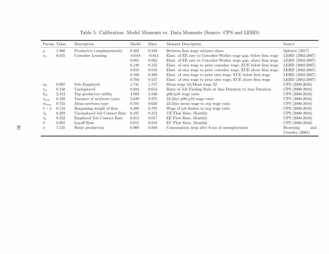
Table 5: Calibration: Model Moments vs. Data Moments (Source: CPS and LEHD)

Param. Value Description Model Data Moment Description Source

ρ 1.966 Productive complementarity 0.482 0.503 Between firm wage variance share Splezter (2017)α1 0.035 Coworker Learning -0.018 -0.014 Elast. of EE rate to Coworker-Worker wage gap, below firm wage LEHD (2002-2007)

0.001 0.002 Elast. of EE rate to Coworker-Worker wage gap, above firm wage LEHD (2002-2007)0.120 0.125 Elast. of own wage to prior coworker wage, EUE below firm wage LEHD (2002-2007)0.018 0.016 Elast. of own wage to prior coworker wage, EUE above firm wage LEHD (2002-2007)0.100 0.289 Elast. of own wage to prior own wage, EUE below firm wage LEHD (2002-2007)0.704 0.557 Elast. of own wage to prior own wage, EUE above firm wage LEHD (2002-2007)

α0 0.007 Solo Employed 1.741 1.717 Mean wage 54/Mean wage 22 CPS (2000-2016)αu 0.150 Unemployed 0.934 0.654 Ratio of Job Finding Rate at 3mo Duration to 1mo Duration CPS (2000-2016)hN 2.412 Top productive ability 4.093 4.546 p90/p10 wage ratio CPS (2000-2016)vnew 0.338 Variance of newborn types 2.639 2.975 22-24yo p90/p10 wage ratio CPS (2000-2016)mnew 0.745 Mean newborn type 0.591 0.620 22-24yo mean wage to avg wage ratio CPS (2000-2016)1− σ 0.118 Bargaining weight of firm 0.486 0.795 Wage of job finders to avg wage ratio CPS (2000-2016)λu 0.293 Unemployed Job Contact Rate 0.197 0.212 UE Flow Rate, Monthly CPS (2000-2016)λe 0.352 Employed Job Contact Rate 0.015 0.017 EE Flow Rate, Monthly CPS (2000-2016)δ 0.007 Layoff Rate 0.011 0.010 EU Flow Rate, Monthly CPS (2000-2016)φ 1.135 Home production 0.900 0.840 Consumption drop after 6 mo of unemployment Browning and

Crossley (2001)

30

4.4 Steady State Distribution of Workers

Figure 2 plots the estimated newborn type distribution and the population type distribution.

Roughly 60% of workers are born as the lowest type, but via learning, as solo employed or

team workers, the fraction of the population that is the lowest type drops to 21.1%. Almost

no workers are born as the highest type, however, through learning, 18.3% of the population

reaches the highest type.

Figure 4 is a contour map of the team distribution. The distribution features many

high-low pairings (schools), many (1,1) teams, and many (7,7) teams. Figure 5 is the corre-

sponding joint pdf. Since there are disproportionately more low-type workers in the economy,

most pairs are formed between low-type workers. Roughly 4.4% of all teams are composed

solely of the lowest type, i.e. (1,1) teams. To understand these sorting patterns, Figure 9

illustrates the hiring policy functions for teams. Type 1 agents are not hired out of unem-

ployment by any team. Type 2 agents displace type 1 agents from teams. Type 3 agents

displace type 1 and type 2 agents from teams. A consequence of learning is that the highest-

productivity team, (7,7), may actually be dissolved in order to pair a lower type agent with

one of the type 7s. This is the case with type 3 agents who are hired by (7,7) teams. The

relative strength of learning and sorting determines how likely a lower-type agent will split

up a pairing of the highest types. Type 4 agents similarly displace type 1, 2, and 3 agents

from teams. Due to learning, type 4 agents will also break up (6,6), (6,7) and (7,7) teams.

Figure 3 illustrates the job flow patterns that arise in steady state. Lowest type individ-

uals have the hardest time obtaining employment, are the most likely to be laid off, and are

also the most likely to switch employers. The highest type individuals are the exact opposite.

To provide more detail on which teams are generating job flows, Figure 8 is a contour map

of the team separation rate. Similar to Figure 9, the greatest separation rates occur among

all teams that have a type 1 worker. These teams are split whenever their firm contacts a

non-type-1 worker. Along the diagonal, separation rates are high, which simply reflects the

fact that learning is a very strong force in the model. Learning is strong enough to disband

(6,6) and (7,7) teams.

Figure 6 plots the distribution of workers across teams. Figure 6 reveals that the lowest

type workers are disproportionately unemployed and working by themselves. As the skill

level rises, the fraction of workers unemployed drops, and the fraction of workers on high-skill

teams rises non-monotonically. The highest type 7 individuals are much more likely to be

paired with a type 5 or type 6 than a fellow type 7. Again, this simply reflects the fact that

31

there are large returns to learning.

To formalize these graphical measures of sorting, Table 6 shows that the Spearman rank

correlation coefficient among worker types is .477, which is consistent with strong worker

complementarity estimates from studies which use different frameworks (e.g. Bonhomme

et al. [2014] and Borovickova and Shimer [2017]). While there is strong sorting, there are

still a large number of workers in ‘schools.’ If we classify a school as a pairing of two workers

who differ by 1 type or more, then approximately 34% of the population is in a school. Figure

7 plots the measure of schools, and nearly 50% of type 1 individuals are being ‘mentored’

by a higher-ranking team member. As we discuss in Section 6, the wage setting mechanism

disincentivizes firms from educating workers by generating a gap between the private and

social returns to learning.

32

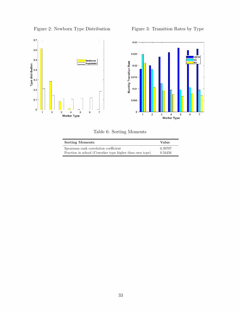
Figure 2: Newborn Type Distribution Figure 3: Transition Rates by Type

Table 6: Sorting Moments

Sorting Moments Value

Spearman rank correlation coefficient 0.39707Fraction in school (Coworker type higher than own type) 0.34456

33

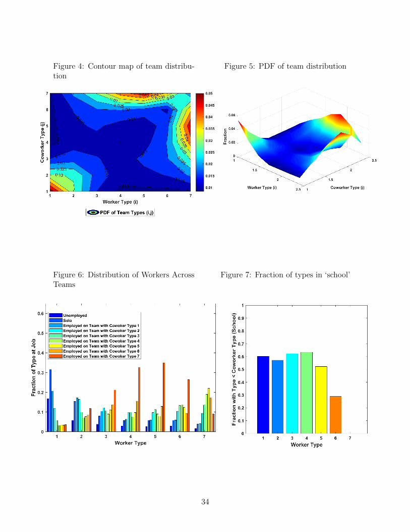
Figure 4: Contour map of team distribu-tion

Figure 5: PDF of team distribution

Figure 6: Distribution of Workers AcrossTeams

Figure 7: Fraction of types in ‘school’

34

Figure 8: Separation Rate by Teams Figure 9: Team hiring policy function

35

5 Sources of Knowledge Diffusion

In this section, we use the calibrated model to understand the determinants of knowledge

diffusion. Table 7 includes results from three counterfactuals, (i) inhibiting all forms of

coworker learning (α1 = 0), but still allowing for worker mobility (λe > 0), (ii) inhibiting

worker mobility (λe = 0), but still allowing for coworker learning (α1 > 0), and (iii) shutting

down both worker mobility and coworker learning (λe = 0, α1 > 0).

Column (1) of Table 7 includes output, sorting, and key moments related to learning

for the baseline U.S. economy. Column (2) of Table 7 shows that if we inhibit all forms of

coworker learning (α1 = 0), but still allowing for worker mobility (λe > 0), output drops by

16.3 percentage points. This implies that coworker learning accounts for 1/6 of U.S. GDP.

When coworker learning is eliminated in Column (2), inequality, measured by the p90

to p10 wage ratio, decreases enormously as the fraction of individuals of the highest type

drops from 18% to 6%. The fraction of high types plummets because high types are no

longer disseminating their knowledge and training lower types. As a consequence, sorting,

measured by the Spearman rank correlation coefficient, increases by 25% when learning is

eliminated, going from .4 to .5. If one minus the spearman rank is interpreted as an index

of ‘mismatch,’ our estimates imply that learning accounts for at least 16% (=.1/(1-.4)) of

measured ‘mismatch.’ This is not to say that learning is actually generating any mismatch.

We will demonstrate in the Planner’s solution that the U.S. allocation of workers to firms is

close to efficient, given the estimated search frictions and learning parameters.

The final three rows of Column (2) include three moments we use to measure sorting

and knowledge diffusion. The counterfactual elimination of coworker learning in Column (2)

implies both (i) an improvement of sorting (an equilibrium result), and (ii) a decline of learn-

ing (by construction, α1 = 0). Regarding the first moment, increased sorting and decreased

learning both serve to augment the share of between-firm wage variance, which increases

by 4 percentage points. The second moment is the correlation of prior coworker wages and

future individual wages among EUE transitioners. Increased sorting and decreased learning

push this moment in opposite directions. Better sorting makes prior coworker wages a bet-

ter predictor of future wages, whereas reduced learning trends to decrease the importance

of prior coworker wages for individual wages. Ultimately, increased sorting dominates and

prior coworker wages become better predictors of future wages of EUE transitioners. Lastly,

low-wage individuals who are paired with high wage individuals are now more likely to switch

employers since they are not learning. This drives the increased sorting.

36

Column (3) shows that relative to the baseline economy, disallowing on-the-job mobility

lowers output by 15.7 percentage points. This implies that mobility is also accountable

for approximately 1/6 of U.S. GDP. With a very strong degree of worker complementarity,

much of the losses from worker mobility are generated by weaker sorting. The Spearman rank

correlation coefficient drops by close to 25%. The share of between firm variance increases

because there are simply twice as many solo workers (with only one wage at the firm),

increasing from 12% to 22%.

Lastly, Column (4) illustrates the turning off both learning and worker mobility would

reduce output by 29%. Despite strong interactions between learning and mobility in the

theory, the impact of jointly eliminating peer effects and mobility is roughly additive. These

three counterfactuals imply that learning and worker mobility both account for 1/3 of U.S.

GDP and are approximately equally important determinants of U.S. output.

Table 7: Relative Importance of Mobility vs. Learning for Knowledge Diffusion and Output

(1) (2) (3) (4)Baseline No Learning

(α1 = 0)No Mobility(λe = 0)

No Mobility andNo Learning

Output 5.81 4.86 4.90 4.08Percent output loss relative to baseline -16.3% -15.7% -29.8%

Wage Dispersion 4.09 3.35 1.65 1.26Spearman rank correlation coefficient 0.40 0.50 0.31 0.28Measure of Solo Employed Workers 0.13 0.12 0.22 0.08

Share of wage variance between firms 0.48 0.52 0.61 0.57Elasticity of own wage with respect to pastcoworker wage, below coworker

0.12 0.20 0.19 0.30

Elasticity of Job to Job transition rate with respectto wage gap (Coworker wage minus individual),below coworker

-0.02 -0.01 0.00 0.00

5.1 Role of Skill Complementarity for Learning and School For-

mation

Figure 10 illustrates the team distribution under the assumption of no production comple-

mentarities between workers, i.e. ρ = 1. The value of a high-type worker is now greater if

that high-type worker is matched with a low-type worker; the high-type worker’s production

is undistorted by their partner’s type, and the the high-type worker will educate the low-type

worker. This discrepancy of types within a team is what we call a school. Once the low-type

37

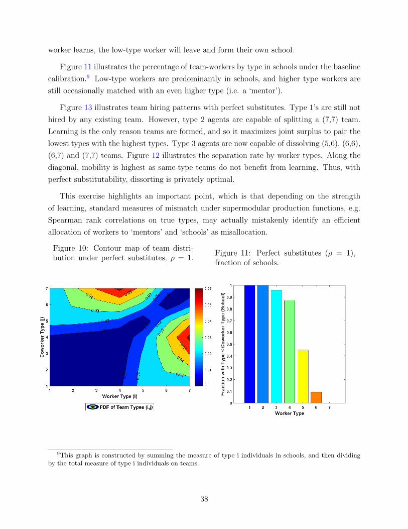
worker learns, the low-type worker will leave and form their own school.

Figure 11 illustrates the percentage of team-workers by type in schools under the baseline

calibration.9 Low-type workers are predominantly in schools, and higher type workers are

still occasionally matched with an even higher type (i.e. a ‘mentor’).

Figure 13 illustrates team hiring patterns with perfect substitutes. Type 1’s are still not

hired by any existing team. However, type 2 agents are capable of splitting a (7,7) team.

Learning is the only reason teams are formed, and so it maximizes joint surplus to pair the

lowest types with the highest types. Type 3 agents are now capable of dissolving (5,6), (6,6),

(6,7) and (7,7) teams. Figure 12 illustrates the separation rate by worker types. Along the

diagonal, mobility is highest as same-type teams do not benefit from learning. Thus, with

perfect substitutability, dissorting is privately optimal.

This exercise highlights an important point, which is that depending on the strength

of learning, standard measures of mismatch under supermodular production functions, e.g.

Spearman rank correlations on true types, may actually mistakenly identify an efficient

allocation of workers to ‘mentors’ and ‘schools’ as misallocation.

Figure 10: Contour map of team distri-bution under perfect substitutes, ρ = 1.

Figure 11: Perfect substitutes (ρ = 1),fraction of schools.

9This graph is constructed by summing the measure of type i individuals in schools, and then dividingby the total measure of type i individuals on teams.

38

Figure 12: Contour map of separationrates with perfect substitutes, ρ = 1.

Figure 13: Team hiring policy functionunder perfect substitutes, ρ = 1.

39

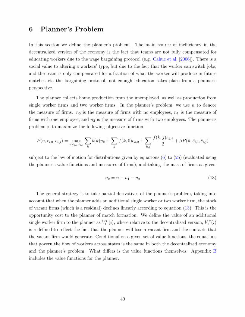
6 Planner’s Problem

In this section we define the planner’s problem. The main source of inefficiency in the

decentralized version of the economy is the fact that teams are not fully compensated for

educating workers due to the wage bargaining protocol (e.g. Cahuc et al. [2006]). There is a

social value to altering a workers’ type, but due to the fact that the worker can switch jobs,

and the team is only compensated for a fraction of what the worker will produce in future

matches via the bargaining protocol, not enough education takes place from a planner’s

perspective.

The planner collects home production from the unemployed, as well as production from

single worker firms and two worker firms. In the planner’s problem, we use n to denote

the measure of firms. n0 is the measure of firms with no employees, n1 is the measure of

firms with one employee, and n2 is the measure of firms with two employees. The planner’s

problem is to maximize the following objective function,

P (u, ei,0, ei,j) = maxu,ei,0,ei,j

∑k

b(k)uk +∑k

f(k, 0)ek,0 +∑k,j

f(k, j)ek,j2

+ βP (u, ei,0, ei,j)

subject to the law of motion for distributions given by equations (6) to (25) (evaluated using

the planner’s value functions and measures of firms), and taking the mass of firms as given

n0 = n− n1 − n2 (13)

The general strategy is to take partial derivatives of the planner’s problem, taking into

account that when the planner adds an additional single worker or two worker firm, the stock

of vacant firms (which is a residual) declines linearly according to equation (13). This is the

opportunity cost to the planner of match formation. We define the value of an additional

single worker firm to the planner as V P1 (i), where relative to the decentralized version, V P

1 (i)

is redefined to reflect the fact that the planner will lose a vacant firm and the contacts that

the vacant firm would generate. Conditional on a given set of value functions, the equations

that govern the flow of workers across states is the same in both the decentralized economy

and the planner’s problem. What differs is the value functions themselves. Appendix B

includes the value functions for the planner.

40

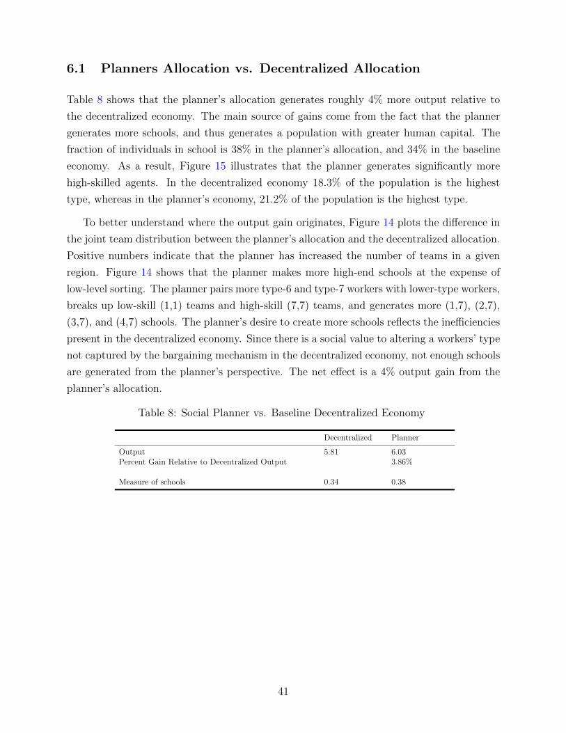
6.1 Planners Allocation vs. Decentralized Allocation

Table 8 shows that the planner’s allocation generates roughly 4% more output relative to

the decentralized economy. The main source of gains come from the fact that the planner

generates more schools, and thus generates a population with greater human capital. The

fraction of individuals in school is 38% in the planner’s allocation, and 34% in the baseline

economy. As a result, Figure 15 illustrates that the planner generates significantly more

high-skilled agents. In the decentralized economy 18.3% of the population is the highest

type, whereas in the planner’s economy, 21.2% of the population is the highest type.

To better understand where the output gain originates, Figure 14 plots the difference in

the joint team distribution between the planner’s allocation and the decentralized allocation.

Positive numbers indicate that the planner has increased the number of teams in a given

region. Figure 14 shows that the planner makes more high-end schools at the expense of

low-level sorting. The planner pairs more type-6 and type-7 workers with lower-type workers,

breaks up low-skill (1,1) teams and high-skill (7,7) teams, and generates more (1,7), (2,7),

(3,7), and (4,7) schools. The planner’s desire to create more schools reflects the inefficiencies

present in the decentralized economy. Since there is a social value to altering a workers’ type

not captured by the bargaining mechanism in the decentralized economy, not enough schools

are generated from the planner’s perspective. The net effect is a 4% output gain from the

planner’s allocation.

Table 8: Social Planner vs. Baseline Decentralized Economy

Decentralized Planner

Output 5.81 6.03Percent Gain Relative to Decentralized Output 3.86%

Measure of schools 0.34 0.38

41

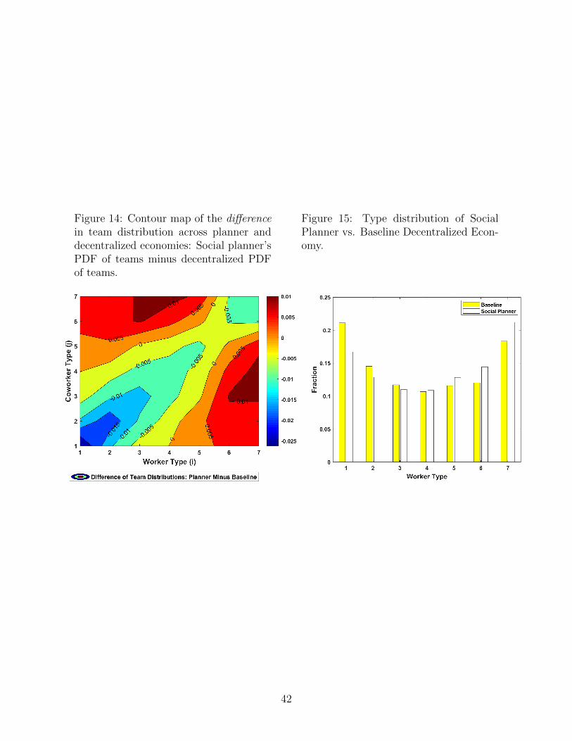
Figure 14: Contour map of the differencein team distribution across planner anddecentralized economies: Social planner’sPDF of teams minus decentralized PDFof teams.

Figure 15: Type distribution of SocialPlanner vs. Baseline Decentralized Econ-omy.

42

7 Conclusion

What role do peer effects, job transitions, and worker complementarities play in the diffusion

of knowledge throughout the US economy? To answer this question, we develop a theory

of teams to measure the way knowledge diffuses within and across firms. Our theoretic

contribution is to extend the frictional sorting framework of Shimer and Smith [2000] to

allow for workers within a firm to influence each other’s knowledge. Workers can search

on-the-job and leave their team to start a new team, carrying some of their knowledge with

them. In contrast to standard sorting models, a firm’s type is no longer exogenous; it is

coworker human capital.

Our quantitative contribution is to estimate peer effects and worker complementarity

using the structure of our model and data from the Longitudinal Employer-Household Dy-

namics (LEHD) database. We indirectly infer the model’s sorting and learning parameters

from three moments in the LEHD, that, when viewed through the lens of our model, directly

inform sorting and learning. Using this methodology, we estimate strong skill complemen-

tarity and strong peer effects.

We then use the estimated model to measure the relative importance of peer effects

and worker mobility for U.S. output. We do so by running counterfactuals that shutdown

learning from coworkers and shutdown job-to-job mobility. Our main finding is that peer-

effects explain roughly 1/6 of GDP in the U.S. while worker mobility explains roughly 1/6

of GDP in the U.S. Thus worker mobility and learning are equally important determinants

of output in the U.S.

Our estimates also imply that learning accounts for at least 16% of measured ‘mismatch,’

which we define be a pairing of a high-type and low-type worker. However, this is not to

say that learning is actually causing any true mismatch; in fact, the planner’s problem

features even more pairings of high and low-type workers (what we also call schools). The

planner’s solution features 38% of individuals in schools, 4% more than in the decentralized

economy, and the planner also manages to produce 4% more than the baseline economy.

With learning, standard measures of sorting are misleading because they do not take into

account the dynamic benefits of coworker interaction.

43

A Expressions for Distributions of Unemployed and

Employed Workers

Similar to the Bellman equations, we split the distribution of type k unemployed workers

within the period into four subperiods: (1) the initial distribution u−k , (2) the distribution

after the learning stage ulearnk , (2) the distribution after births and deaths uk (the start of

the search stage), (3) the distribution after search outcomes are realized usearchk , and (4)

the distribution after dismissals occur, u+k . u+

k becomes the initial distribution for the next

period, u−k . An equilibrium is a fixed point of this mapping.

A.1 Learning

After dismissal, production occurs, and then types are realized according to the function g,

which takes as inputs the agent’s type and the coworker’s type (if an agent is unemployed,

the coworker type is denoted ‘u’, if an agent is employed alone, the coworker type is denoted

‘0’, and if an agent is employed with a coworker of type j, then the coworker type is simply

‘j’). Let u−j denote the mass of unemployed agents at the start of the period. Let e−k0and

e−i,j be similarly defined. The evolution of types for the unemployed is therefore given by,

ulearnk = u−k +∑j 6=k

u−j gu(k | j)−∑j 6=k

u−k gu(j | k) (14)

The evolution of types for agents at single worker firms is therefore given by,

elearnk,0 = e−k,0 +∑j 6=k

e−j,0g0(k | j)−∑j 6=k

e−k,0g0(j | k) (15)

The evolution of types for workers at two worker firms is therefore given by,

elearnk,l = e−k,l +∑

(i,j)6=(k,l)

e−i,jgj(k | i)gi(l | j)−∑

(i,j) 6=(k,l)

e−k,lgl(i | k)gk(j | l) (16)

44

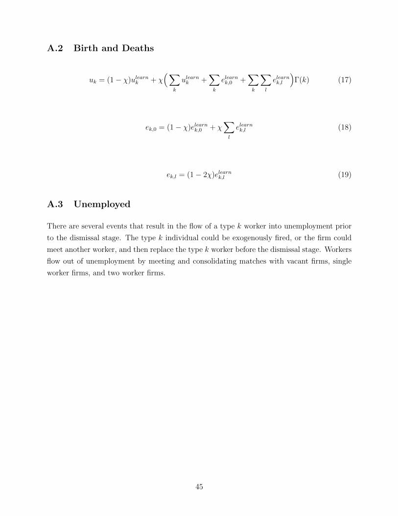
A.2 Birth and Deaths

uk = (1− χ)ulearnk + χ(∑

k

ulearnk +∑k

elearnk,0 +∑k

∑l

elearnk,l

)Γ(k) (17)

ek,0 = (1− χ)elearnk,0 + χ∑l

elearnk,l (18)

ek,l = (1− 2χ)elearnk,l (19)

A.3 Unemployed

There are several events that result in the flow of a type k worker into unemployment prior

to the dismissal stage. The type k individual could be exogenously fired, or the firm could

meet another worker, and then replace the type k worker before the dismissal stage. Workers

flow out of unemployment by meeting and consolidating matches with vacant firms, single

worker firms, and two worker firms.

45

usearchk =uk − ukλuF0

FI(V1(k)−Π0 − U(k) > 0)

− uk∑i

λuei,0

FI(V2(k, i)− U(k)− V1(i) > 0)

− uk∑i

∑j

(λuei,j

2FI(max{V2(k, j) + U(i)− U(k)− V2(i, j), V2(i, k) + U(j)− U(k)− V2(i, j)} > 0))

︸ ︷︷ ︸worker meets firm (i,j) and is hired

+∑i

ek,lλuuiF

I(max{V2(k, i) + U(l)− U(i)− V2(k, l), V2(i, l) + U(k)− U(i)− V2(k, l)} > 0)︸ ︷︷ ︸firm (k,l) meets unemployed and hires

× I(V2(i, l) + U(k)− U(i)− V2(k, l) > V2(k, i) + U(l)− U(i)− V2(k, l))︸ ︷︷ ︸firm replaces k

+∑i

ek,lλeei,0

FI(max{V2(k, i) + U(l)− (V1(i)−Π0)− V2(k, l), V2(i, l) + U(k)− (V1(i)−Π0)− V2(k, l)} > 0)︸ ︷︷ ︸

firm (k,l) meets solo and hires

× I(V2(i, l) + U(k)− (V1(i)−Π0)− V2(k, l) > V2(k, i) + U(l)− (V1(i)−Π0)− V2(k, l))︸ ︷︷ ︸firm replaces k

+∑i

∑j

ek,lλeei,j

FI(max{V2(k, i) + U(l)− (V2(i, j)− V1(j))− V2(k, l), V2(i, l) + U(k)− (V2(i, j)− V1(j))− V2(k, l)} > 0)︸ ︷︷ ︸

firm (k,l) meets agent i in (i,j) match

× I(V2(i, l) + U(k)− (V2(i, j)− V1(j))− V2(k, l) > V2(k, i) + U(l)− (V2(i, j)− V1(j))− V2(k, l))︸ ︷︷ ︸firm replaces k

+ δ(ek,0 +

∑i

ek,i

)(20)

A.4 Solo Employed

The flow equation for single worker firms incorporates many events; flows out include normal

exogenous layoffs, team formation, and on-the-job-search. Flows in include exogenous layoffs

(of one member of a two worker firm), new hires, and poaching from teams.

46

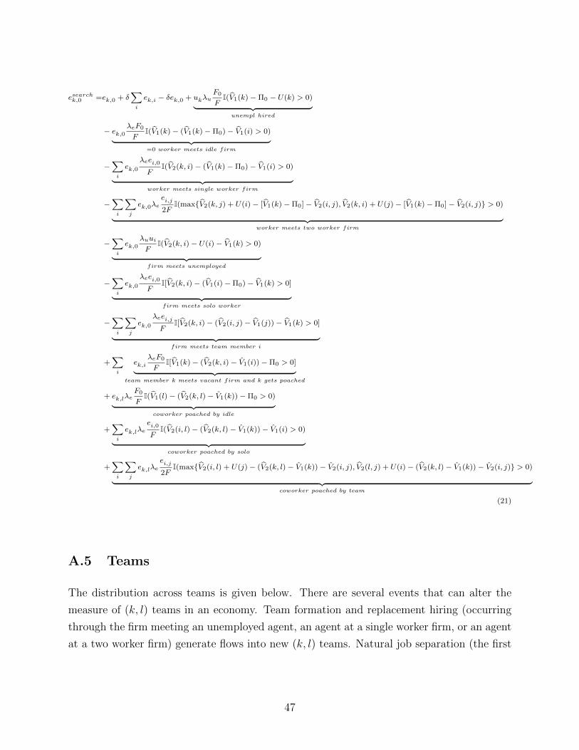
esearchk,0 =ek,0 + δ∑i

ek,i − δek,0 + ukλuF0

FI(V1(k)−Π0 − U(k) > 0)︸ ︷︷ ︸unempl hired

− ek,0λeF0

FI(V1(k)− (V1(k)−Π0)− V1(i) > 0)︸ ︷︷ ︸=0 worker meets idle firm

−∑i

ek,0λeei,0

FI(V2(k, i)− (V1(k)−Π0)− V1(i) > 0)︸ ︷︷ ︸

worker meets single worker firm

−∑i

∑j

ek,0λeei,j

2FI(max{V2(k, j) + U(i)− [V1(k)−Π0]− V2(i, j), V2(k, i) + U(j)− [V1(k)−Π0]− V2(i, j)} > 0)

︸ ︷︷ ︸worker meets two worker firm

−∑i

ek,0λuui

FI(V2(k, i)− U(i)− V1(k) > 0)︸ ︷︷ ︸

firm meets unemployed

−∑i

ek,0λeei,0

FI[V2(k, i)− (V1(i)−Π0)− V1(k) > 0]︸ ︷︷ ︸firm meets solo worker

−∑i

∑j

ek,0λeei,j

FI[V2(k, i)− (V2(i, j)− V1(j))− V1(k) > 0]

︸ ︷︷ ︸firm meets team member i

+∑i

ek,iλeF0

FI[V1(k)− (V2(k, i)− V1(i))−Π0 > 0]︸ ︷︷ ︸

team member k meets vacant firm and k gets poached

+ ek,lλeF0

FI(V1(l)− (V2(k, l)− V1(k))−Π0 > 0)︸ ︷︷ ︸coworker poached by idle

+∑i

ek,lλeei,0

FI(V2(i, l)− (V2(k, l)− V1(k))− V1(i) > 0)︸ ︷︷ ︸coworker poached by solo

+∑i

∑j

ek,lλeei,j

2FI(max{V2(i, l) + U(j)− (V2(k, l)− V1(k))− V2(i, j), V2(l, j) + U(i)− (V2(k, l)− V1(k))− V2(i, j)} > 0)

︸ ︷︷ ︸coworker poached by team

(21)

A.5 Teams

The distribution across teams is given below. There are several events that can alter the

measure of (k, l) teams in an economy. Team formation and replacement hiring (occurring

through the firm meeting an unemployed agent, an agent at a single worker firm, or an agent

at a two worker firm) generate flows into new (k, l) teams. Natural job separation (the first

47

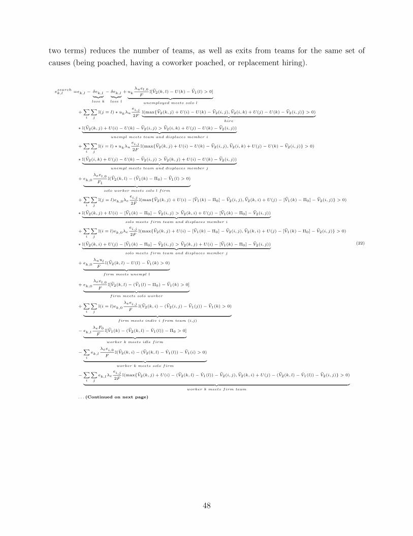
two terms) reduces the number of teams, as well as exits from teams for the same set of

causes (being poached, having a coworker poached, or replacement hiring).

esearchk,l =ek,l − δek,l︸ ︷︷ ︸

lose k

− δek,l︸ ︷︷ ︸lose l

+uk

λuel,0

FI[V2(k, l)− U(k)− V1(l) > 0]︸ ︷︷ ︸

unemployed meets solo l

+∑i

∑j

I(j = l) ∗ ukλu

ei,j

2FI(max{V2(k, j) + U(i)− U(k)− V2(i, j), V2(i, k) + U(j)− U(k)− V2(i, j)} > 0)︸ ︷︷ ︸

hire

∗ I(V2(k, j) + U(i)− U(k)− V2(i, j) > V2(i, k) + U(j)− U(k)− V2(i, j))︸ ︷︷ ︸unempl meets team and displaces member i

+∑i

∑j

I(i = l) ∗ ukλu

ei,j

2FI(max{V2(k, j) + U(i)− U(k)− V2(i, j), V2(i, k) + U(j)− U(k)− V2(i, j)} > 0)

∗ I(V2(i, k) + U(j)− U(k)− V2(i, j) > V2(k, j) + U(i)− U(k)− V2(i, j))︸ ︷︷ ︸unempl meets team and displaces member j

+ ek,0

λeel,0

F1

I(V2(k, l)− (V1(k)− Π0)− V1(l) > 0)︸ ︷︷ ︸solo worker meets solo l firm

+∑i

∑j

I(j = l)ek,0λe

ei,j

2FI(max{V2(k, j) + U(i)− [V1(k)− Π0]− V2(i, j), V2(k, i) + U(j)− [V1(k)− Π0]− V2(i, j)} > 0)

∗ I(V2(k, j) + U(i)− [V1(k)− Π0]− V2(i, j) > V2(k, i) + U(j)− [V1(k)− Π0]− V2(i, j))︸ ︷︷ ︸solo meets firm team and displaces member i

+∑i

∑j

I(i = l)ek,0λe

ei,j

2FI(max{V2(k, j) + U(i)− [V1(k)− Π0]− V2(i, j), V2(k, i) + U(j)− [V1(k)− Π0]− V2(i, j)} > 0)

∗ I(V2(k, i) + U(j)− [V1(k)− Π0]− V2(i, j) > V2(k, j) + U(i)− [V1(k)− Π0]− V2(i, j))︸ ︷︷ ︸solo meets firm team and displaces member j

+ ek,0

λuul

FI(V2(k, l)− U(l)− V1(k) > 0)︸ ︷︷ ︸

firm meets unempl l

+ ek,0

λeel,0

FI[V2(k, l)− (V1(l)− Π0)− V1(k) > 0]︸ ︷︷ ︸firm meets solo worker

+∑i

∑j

I(i = l)ek,0

λeei,j

FI(V2(k, i)− (V2(i, j)− V1(j))− V1(k) > 0)

︸ ︷︷ ︸firm meets indiv i from team (i,j)

− ek,l

λeF0

FI[V1(k)− (V2(k, l)− V1(l))− Π0 > 0]︸ ︷︷ ︸worker k meets idle firm

−∑i

ek,l

λeei,0

FI(V2(k, i)− (V2(k, l)− V1(l))− V1(i) > 0)

︸ ︷︷ ︸worker k meets solo firm

−∑i

∑j

ek,lλe

ei,j

2FI(max{V2(k, j) + U(i)− (V2(k, l)− V1(l))− V2(i, j), V2(k, i) + U(j)− (V2(k, l)− V1(l))− V2(i, j)} > 0)

︸ ︷︷ ︸worker k meets firm team

. . . (Continued on next page)

(22)

48

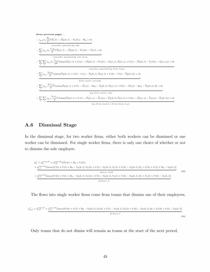
(from previous page) . . .

− ek,lλeF0

FI(V1(l)− (V2(k, l)− V1(k))− Π0 > 0)︸ ︷︷ ︸coworker poached by idle

−∑i

ek,lλe

ei,0

FI(V2(i, l)− (V2(k, l)− V1(k))− V1(i) > 0)

︸ ︷︷ ︸coworker poached by solo firm

−∑i

∑j

ek,lλe

ei,j

2FI(max{V2(i, l) + U(j)− (V2(k, l)− V1(k))− V2(i, j), V2(l, j) + U(i)− (V2(k, l)− V1(k))− V2(i, j)} > 0)

︸ ︷︷ ︸coworker poached by firm team

−∑i

ek,l

λuui

FI(max{V2(k, i) + U(l)− U(i)− V2(k, l), V2(i, l) + U(k)− U(i)− V2(k, l)} > 0)

︸ ︷︷ ︸firm meets unempl

−∑i

ek,l

λeei,0

FI(max{V2(k, i) + U(l)− (V1(i)− Π0)− V2(k, l), V2(i, l) + U(k)− (V1(i)− Π0)− V2(k, l), 0} > 0)

︸ ︷︷ ︸my firm meets solo

−∑i

∑j

ek,l

λeei,j

FI(max{V2(k, i) + U(l)− (V2(i, j)− V1(j))− V2(k, l), V2(i, l) + U(k)− (V2(i, j)− V1(j))− V2(k, l)} > 0)︸ ︷︷ ︸

my firm meets i from team (i,j)

A.6 Dismissal Stage

In the dismissal stage, for two worker firms, either both workers can be dismissed or one

worker can be dismissed. For single worker firms, there is only one choice of whether or not

to dismiss the sole employee.

u+k = u

searchk + e

searchk,0 I(V1(k) < Π0 + U(k))

+ esearchk,l I[max{U(k) + U(l) + Π0 − V2(k, l), V1(k) + U(l)− V2(k, l), V1(l) + U(k)− V2(k, l), 0} = U(k) + U(l) + Π0 − V2(k, l)]︸ ︷︷ ︸

dimiss both

+ esearchk,l I[max{U(k) + U(l) + Π0 − V2(k, l), V1(k) + U(l)− V2(k, l), V1(l) + U(k)− V2(k, l), 0} = V1(l) + U(k)− V2(k, l)]︸ ︷︷ ︸

dismiss k

(23)

The flows into single worker firms come from teams that dismiss one of their employees,

e+k,0 = e

searchk,0 + e

searchk,l I[max{U(k) + U(l) + Π0 − V2(k, l), V1(k) + U(l)− V2(k, l), V1(l) + U(k)− V2(k, l), 0} = V1(k) + U(l)− V2(k, l)]︸ ︷︷ ︸

dismiss l

(24)

Only teams that do not dimiss will remain as teams at the start of the next period,

49

e+k,l = e

searchk,l + e

searchk,l I[max{U(k) + U(l) + Π0 − V2(k, l), V1(k) + U(l)− V2(k, l), V1(l) + U(k)− V2(k, l), 0} = 0]︸ ︷︷ ︸

no dismissal

(25)

The values u+k , e+

k,0, and e+k,l become next period’s starting values u−k , e−k,0, and e−k,l,

respectively. An equilibrium is a fixed point of this mapping.

B Planner’s Problem

This section includes the planner’s continuation values for both single-worker firms and two-

worker firms net of the opportunity cost of creating those jobs (the opportunity cost is the

value of the contacts forfeited by losing a vacant firm), as well as the planner’s continuation

value for the unemployed. The opportunity cost of creating a match includes the forfeited

contacts of a vacant firm:

Planners Opportunity Cost of Match =∑i

λuuin

max{V P1 (i)− UP (i), 0}

+∑i

λeei,0n

max{V P1 (i)− V P

1 (i), 0}+∑i

∑j

λeei,jn

max{V P1 (i) + V P

1 (j)− V P2 (i, j), 0}

The value of an unemployed worker to the planner is,

UP (k) = b(k) + βEk+

[UP (k+)

+ λun0

nmax{V P

1 (k+)− UP (k+), 0}

+ λu∑i

ei,0n

max{V P2 (k+, i)− V P

1 (i)− UP (k+), 0}

+ λu∑i

∑j

ei,j2n

max{V P2 (k+, i) + U(j)− V P

2 (i, j)− UP (k+),

V P2 (k+, j) + UP (i)− V P

2 (i, j)− UP (k+), 0}]

50

The joint value of an additional single worker firm to the planner is,

V P1 (k) = f(k, 0) + βEk+{V P

1 (k+)

+ λen0n

max{V P1 (k+)− V P

1 (k+), 0}

+ λe∑i

ei,0n

max{V P2 (k+, i)− V P

1 (i)− V P1 (k+), 0}

+ λe∑i

∑j

ei,j2n

max{V P2 (k+, i) + UP (j)− V P

2 (i, j)− V P1 (k+), V P

2 (k+, j) + UP (i)− V P2 (i, j)− V P

1 (k+), 0}

+∑i

λuuin

max{V P2 (i, k+)− UP (i)− V P

1 (k+), 0}

+∑i

λeei,0n

max{V P2 (i, k+)− V P

1 (i)− V P1 (k+), 0}

+∑i

∑j

λeei,jn

max{V P2 (i, k+) + V P

1 (j)− V P2 (i, j)− V P

1 (k+), 0}

−∑i

λuuin

max{V P1 (i)− UP (i), 0} −

∑i

λeei,0n

max{V P1 (i)− V P

1 (i), 0} −∑i

∑j

λeei,jn

max{V P1 (i) + V P

1 (j)− V P2 (i, j), 0}︸ ︷︷ ︸

opportunity cost to planner

+ δ(UP (k)− V P1 (k))}

51

The joint value of a two worker firm to the planner is,

V P2 (k, l) = f(k, l) + βEk+,l+{VP1 (k+, l+)

+ λen0

nmax{V P1 (k+) + V P1 (l+)− V P2 (k+, l+), 0}

+ λe∑i

ei,0

nmax{V P2 (k+, i) + V P1 (l+)− V P2 (k+, l+)− V P1 (i), 0}

+ λe∑i

∑j

ei,j

2nmax{V P2 (k+, i) + V P1 (l+) + UP (j)− V P2 (k+, l+)− V P2 (i, j), V P2 (k+, j) + V P1 (l+) + UP (i)− V P2 (k+, l+)− V P2 (i, j), 0}

︸ ︷︷ ︸k meets (i,j) team

+ λen0

nmax{V P1 (l+) + V P1 (k+)− V P2 (k+, l+), 0}

+∑i

λeei,0

nmax{V P2 (l+, i) + V P1 (k+)− V P2 (k+, l+)− V P1 (i), 0}

+∑i

∑j

λeei,j

2nmax{V P2 (l+, i) + V P1 (k+) + UP (j)− V P2 (k+, l+)− V P2 (i, j), V P2 (l+, j) + V P1 (k+) + UP (i)− V P2 (k+, l+)− V P2 (i, j), 0}

︸ ︷︷ ︸l meets (i,j) team

+∑i

λuui

nmax{V P2 (k+, i) + UP (l+)− UP (i)− V P2 (k+, l+), V P2 (i, l+) + UP (k+)− UP (i)− V P2 (k+, l+), 0}

+∑i

λeei,0

nmax{V P2 (k+, i) + UP (l+)− V P1 (i)− V P2 (k+, l+), V P2 (i, l+) + UP (k+)− V P1 (i)− V P2 (k+, l+), 0}

+∑i

∑j

λeei,j

nmax{V P2 (k+, i) + UP (l+)− (V P2 (i, j)− V P1 (j))− V P2 (k+, l+), V P2 (i, l+) + UP (k+)− (V P2 (i, j)− V P1 (j))− V P2 (k+, l+), 0}

−∑i

λuui

nmax{V P1 (i)− UP (i), 0}

−∑i

λeei,0

nmax{V P1 (i)− V P1 (i), 0}

−∑i

∑j

λeei,j

nmax{V P1 (i) + V P1 (j)− V P2 (i, j), 0}

+ δ(V P1 (k+) + UP (l+)− V P2 (k+, l+))

+ δ(V P1 (l+) + UP (k+)− V P2 (k+, l+))}

C Data Appendix

Our unit of observation is a State Employment Identification Number (SEIN), and we focus

on single-unit firms within a state, meaning that the firm only had one physical plant location

in that state and it thus corresponds to the SEIN in the LEHD database. We identify primary

employers as the SEINs which pay the individual the most in a given year. Coworker wages

are measured as the quarter 4 wage bill net of an individual’s own wage divided by the

number of employees in quarter 4 at the SEIN.

To be in our base dataset, one must have worked at least 260 hours (one quarter, part-

52

time) at least once between 1998 and 2008. These are similar restrictions used in Guvenen

et al. [2015]. Our variables are deflated by the BLS CPI, and we winsorize the top 1% of all

continuous variables. We define an individual to be full-year employed if they earn above

$1,000 in each quarter of the year. We define an individual to be non-employed in a given

quarter if they earn less than $1,000. Our results are not sensitive to this cutoff.

Individuals are in the sample if they work at single-unit firm (meaning all the workers are

working in the same physical area) with between 2 and 250 employees, are prime-age, and are

male. The sample covers 2001 to 2008, but based on the forward lags of the variables used,

the last cohort used for job transitions is 2006, with outcomes measured in 2008. An EUE

transition is defined as a full-year of employment in year t, one quarter of non-employment

in year t+1, and full-year employment in year t+2.

D Data Description: Brazilian Data

In this section, we verify our results on Brazilian data. We conduct several important

robustness checks: (i) we specify coworker wages within an occupation, (ii) we follow workers

over a 4 year horizon, (iii) we isolate industry switchers, (iv) we compare our results to

standard methods, and (v) we look at learning based on different summary measures of the

firm’s workforce, including the different deciles of the coworker wage distribution.10

We use the RAIS database from Brazil, which is an annual census of the universe of formal

firms, including the establishments of those firms, both public and private, in Brazil.11 We

use a sample of this data from the state of Bahia in Brazil which includes approximately 37

million person-year observations. Bahia is the fourth largest state in Brazil with a population

of approximately 15 million individuals. Our sample of data spans 1998 to 2010.

Unlike the US administrative data (such as the LEHD), RAIS includes occupation data.12

We are therefore able to isolate coworkers within a given firm and 2-digit occupation code. We

10All RAIS results contained in this paper were run on IPEA servers in accordance with MTE guidelines.11In English RAIS roughly stands for Annual Relation of Social Information (RAIS). For more discussion

of the data, see Araujo [2014] and Engbom and Moser [2016].12Brazil’s occupational classification system is called the CBO (Classificacao Brasileira de Ocupacoes), and

is discussed at length in Muendler et al. [2004]. The CBO is more detailed than international occupationclassifications, and Muendler et al. [2004] maps the CBO into the international standard classification ISCO(International Standard Classification of Occupations). As Muendler et al. [2004] describe, “At the finestlevel, CBO-94 defines an individual occupation as a category that unifies jobs which are fundamentallysimilar with regard to their ‘content’ and ‘skill requirements.”’

53

believe the jobs that are being carried out within these establishment level 2-digit occupation

bins have similar skill requirements.

Another advantage of the Brazilian data is that we observe the reason for job transition

(retirement, transfer, fired, quit). We are therefore able to condition on the worker being

fired.

D.1 Empirical Approach: Brazilian Data

Our empirical approach follows Section 4.2. We therefore focus on the following sample:

Prime age (24 to 65) males with at least 1 year of tenure who must have positive earnings

in year t and t+2 from different primary employers (the primary employer is simply the

establishment that paid the worker the most in a given year); moreover, they must be fired

and switch primary employers in year t+1 and have at least one quarter of non-employment

in year t+1. We require that they have at least one coworker within the establishment,

within the same 2-digit occupation. We further condition on the individuals earning at least

100 real per month (in 2010 real), in order to get rid of workers who are earning below the

minimum wage and likely to be in the informal sector.

All variables are winsorized at the top 1%, and nominal variables are deflated using the

Brazilian CPI. Let wi,t denote an individual’s raw average monthly wage at his/her primary

employer at date t. Our main outcome of interest is the log of this wage, wi,t = ln(wi,t).

Furthermore, define w−i,t as the raw average monthly wage of the coworkers of an individual

at his/her primary employer at date t within the same 2-digit occupation. Let w−i,t =

ln(w−i,t) denote the log of this variable.

D.2 Estimation Equation: Brazilian Data

Let i index people and t index years. Let Yi,t+2 be the dependent variable of interest, e.g. the

individual i’s log average monthly wage year t+2 or the log average monthly wage of workers

in a given occupation at individual i’s primary employer in year t+2. The primary employer

is defined as the employer that paid the worker the most in a given year. We estimate the

following specifications on the Brazilian data:

Yi,t+2 = β0 + γt + β1wi,t + β2w−i,t + ΓXi,t + εi,t

54

D.3 Baseline Specifications: Brazilian Data

Table 9 illustrates the impact of coworker wages, within the same establishment and same

2-digit occupation, on the subsequent wages of an individual after a spell of non-employment.

The independent covariates are measured as of date t, and the outcome variable is an in-

dividual’s log average monthly wage at their new employer at date t+2. Each specification

includes fixed effects for contract type, year, sector (1 digit), occupation (2 digit), as well as

quadratics in age and tenure.

Column (1) reveals a strong correlation between coworker wages and an individual’s

future wages for EUE transitioners. This coefficient is about two and a half times smaller

than the same coefficient in the LEHD data. If an individual’s coworkers earn 10% more,

the individual will earn, on average, a .16% greater wage upon reemployment. Column (2)

restricts the sample to EUE transitioners who were initially below the mean wage, within

their occupation at their establishment. Consistent with the LEHD, the effects of coworker

wages are roughly two times as large as the population average effect. Column (4) focuses

on workers above the mean wage, and the effect is indiscernible from zero.

To check whether we are measuring general versus industry-specific or establishment-

specific forms of human capital, Column (4) focuses on those who switch 1-digit sectors in

their EUE transition.13 Column (4) reveals that the elasticity of future wage with respect

to coworker wages is quite stable, even among industry switchers. This suggests that our

measures of peer-effects are capturing general human capital accumulation, as opposed to

other forms of human capital accumulation.

As another test of whether we are measuring human capital or some other short-term

characteristic of the prior employer, Table 10 repeats our regressions with different horizons

ranging from 1 year after job loss (reemployed at t+2, lost job at t+1), to 4 years after job

loss, (reemployed at t+5, lost job at t+1). Column (1) includes the 1 year horizon, Column

(2) is the 2 year horizon, Column (3) is the 3 year horizon, and Column (4) is the 4 year

horizon. Table 10 reveals a fairly stable impact of coworker wages on future individual wages.

The impact of coworker wages on future individual wages remains significant 4 years after

13These sectors include: 1 ”Metal & Mineral Manufacturing”; 2 ”Machinery & Eletronics Manufacturing”3 ”Others Manufacturing”; 4 ”Chemical Manufacturing”; 5 ”Textile Manufacturing”; 6 ”Food & DrinkManufacturing” 7 ”Construction” ; 8 ”Retail Trade”; 9 ”Wholesale Trade” ; 10 ”Finance & InsuranceServices” ; 11 ”Real State Services” ; 12 ”Traffic & Technical Services” ; 13 ”Accommodation & FoodServices”; 14 ”Health & Social Services” ; 15 ”Educational Services” ; 16 ”Government” ; 17 ”Agriculture,etc”

55

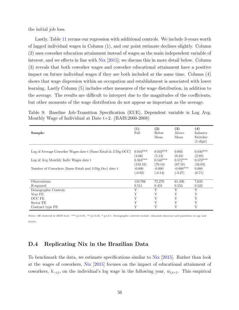
the initial job loss.

Lastly, Table 11 reruns our regression with additional controls. We include 3-years worth

of lagged individual wages in Column (1), and our point estimate declines slightly. Column

(2) uses coworker education attainment instead of wages as the main independent variable of

interest, and we effects in line with Nix [2015]; we discuss this in more detail below. Column

(3) reveals that both coworker wages and coworker educational attainment have a positive

impact on future individual wages if they are both included at the same time. Column (4)

shows that wage dispersion within an occupation and establishment is associated with lower

learning. Lastly Column (5) includes other measures of the wage distribution, in addition to

the average. The results are difficult to interpret due to the magnitudes of the coefficients,

but other moments of the wage distribution do not appear as important as the average.

Table 9: Baseline Job-Transition Specification (EUE). Dependent variable is Log Avg.Monthly Wage of Individual at Date t+2. (RAIS:2000-2008)

(1) (2) (3) (4)Sample: Full Below

MeanAboveMean

IndustrySwitcher(1-digit)

Log of Average Coworker Wages date t (Same Estab & 2-Dig OCC) 0.016*** 0.032*** 0.003 0.046***(4.06) (5.13) (0.34) (2.88)

Log of Avg Monthly Indiv Wages date t 0.563*** 0.543*** 0.572*** 0.573***(133.10) (70.14) (67.55) (34.03)

Number of Coworkers (Same Estab and 2-Dig Occ) date t -0.000 -0.000 -0.000*** 0.000(-0.92) (-0.14) (-3.27) (0.71)

Observations 133,706 72,270 61,436 7,633R-squared 0.511 0.455 0.553 0.522Demographic Controls Y Y Y YYear FE Y Y Y YOCC FE Y Y Y YSector FE Y Y Y YContract type FE Y Y Y Y

Notes: SE clustered at SEIN level. *** p<0.01, ** p<0.05, * p<0.1. Demographic controls include: education dummies and quadratics in age and

tenure.

D.4 Replicating Nix in the Brazilian Data

To benchmark the data, we estimate specifications similar to Nix [2015]. Rather than look

at the wages of coworkers, Nix [2015] focuses on the impact of educational attainment of

coworkers, h−i,t, on the individual’s log wage in the following year, wi,t+1. This empirical

56

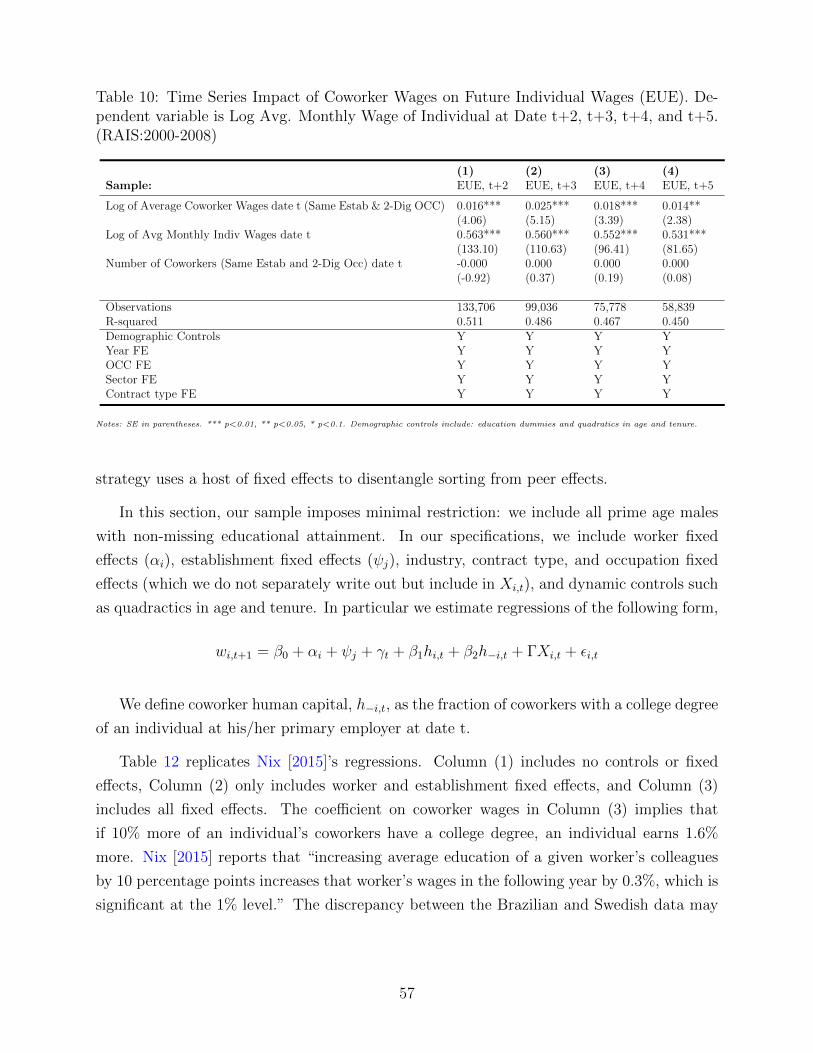
Table 10: Time Series Impact of Coworker Wages on Future Individual Wages (EUE). De-pendent variable is Log Avg. Monthly Wage of Individual at Date t+2, t+3, t+4, and t+5.(RAIS:2000-2008)

(1) (2) (3) (4)Sample: EUE, t+2 EUE, t+3 EUE, t+4 EUE, t+5

Log of Average Coworker Wages date t (Same Estab & 2-Dig OCC) 0.016*** 0.025*** 0.018*** 0.014**(4.06) (5.15) (3.39) (2.38)

Log of Avg Monthly Indiv Wages date t 0.563*** 0.560*** 0.552*** 0.531***(133.10) (110.63) (96.41) (81.65)

Number of Coworkers (Same Estab and 2-Dig Occ) date t -0.000 0.000 0.000 0.000(-0.92) (0.37) (0.19) (0.08)

Observations 133,706 99,036 75,778 58,839R-squared 0.511 0.486 0.467 0.450Demographic Controls Y Y Y YYear FE Y Y Y YOCC FE Y Y Y YSector FE Y Y Y YContract type FE Y Y Y Y

Notes: SE in parentheses. *** p<0.01, ** p<0.05, * p<0.1. Demographic controls include: education dummies and quadratics in age and tenure.

strategy uses a host of fixed effects to disentangle sorting from peer effects.

In this section, our sample imposes minimal restriction: we include all prime age males

with non-missing educational attainment. In our specifications, we include worker fixed

effects (αi), establishment fixed effects (ψj), industry, contract type, and occupation fixed

effects (which we do not separately write out but include in Xi,t), and dynamic controls such

as quadractics in age and tenure. In particular we estimate regressions of the following form,

wi,t+1 = β0 + αi + ψj + γt + β1hi,t + β2h−i,t + ΓXi,t + εi,t

We define coworker human capital, h−i,t, as the fraction of coworkers with a college degree

of an individual at his/her primary employer at date t.

Table 12 replicates Nix [2015]’s regressions. Column (1) includes no controls or fixed

effects, Column (2) only includes worker and establishment fixed effects, and Column (3)

includes all fixed effects. The coefficient on coworker wages in Column (3) implies that

if 10% more of an individual’s coworkers have a college degree, an individual earns 1.6%

more. Nix [2015] reports that “increasing average education of a given worker’s colleagues

by 10 percentage points increases that worker’s wages in the following year by 0.3%, which is

significant at the 1% level.” The discrepancy between the Brazilian and Swedish data may

57

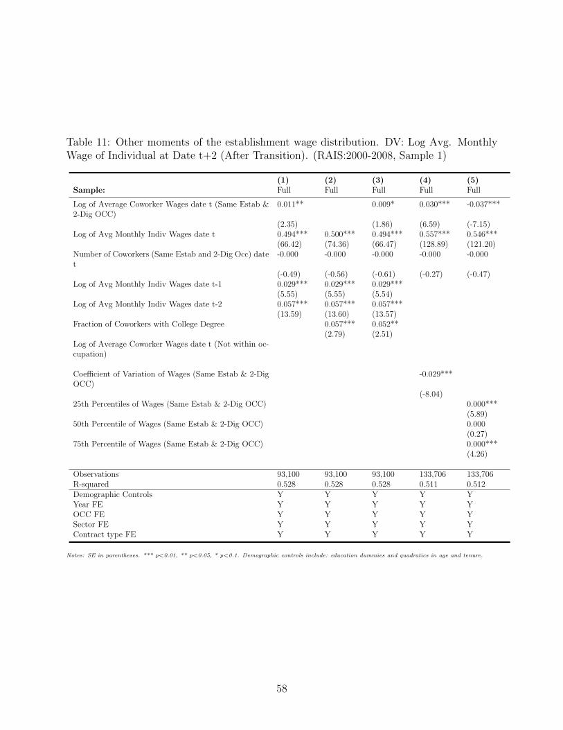
Table 11: Other moments of the establishment wage distribution. DV: Log Avg. MonthlyWage of Individual at Date t+2 (After Transition). (RAIS:2000-2008, Sample 1)

(1) (2) (3) (4) (5)Sample: Full Full Full Full Full

Log of Average Coworker Wages date t (Same Estab &2-Dig OCC)

0.011** 0.009* 0.030*** -0.037***

(2.35) (1.86) (6.59) (-7.15)Log of Avg Monthly Indiv Wages date t 0.494*** 0.500*** 0.494*** 0.557*** 0.546***

(66.42) (74.36) (66.47) (128.89) (121.20)Number of Coworkers (Same Estab and 2-Dig Occ) datet

-0.000 -0.000 -0.000 -0.000 -0.000

(-0.49) (-0.56) (-0.61) (-0.27) (-0.47)Log of Avg Monthly Indiv Wages date t-1 0.029*** 0.029*** 0.029***

(5.55) (5.55) (5.54)Log of Avg Monthly Indiv Wages date t-2 0.057*** 0.057*** 0.057***

(13.59) (13.60) (13.57)Fraction of Coworkers with College Degree 0.057*** 0.052**

(2.79) (2.51)Log of Average Coworker Wages date t (Not within oc-cupation)

Coefficient of Variation of Wages (Same Estab & 2-DigOCC)

-0.029***

(-8.04)25th Percentiles of Wages (Same Estab & 2-Dig OCC) 0.000***

(5.89)50th Percentile of Wages (Same Estab & 2-Dig OCC) 0.000

(0.27)75th Percentile of Wages (Same Estab & 2-Dig OCC) 0.000***

(4.26)

Observations 93,100 93,100 93,100 133,706 133,706R-squared 0.528 0.528 0.528 0.511 0.512Demographic Controls Y Y Y Y YYear FE Y Y Y Y YOCC FE Y Y Y Y YSector FE Y Y Y Y YContract type FE Y Y Y Y Y

Notes: SE in parentheses. *** p<0.01, ** p<0.05, * p<0.1. Demographic controls include: education dummies and quadratics in age and tenure.

58

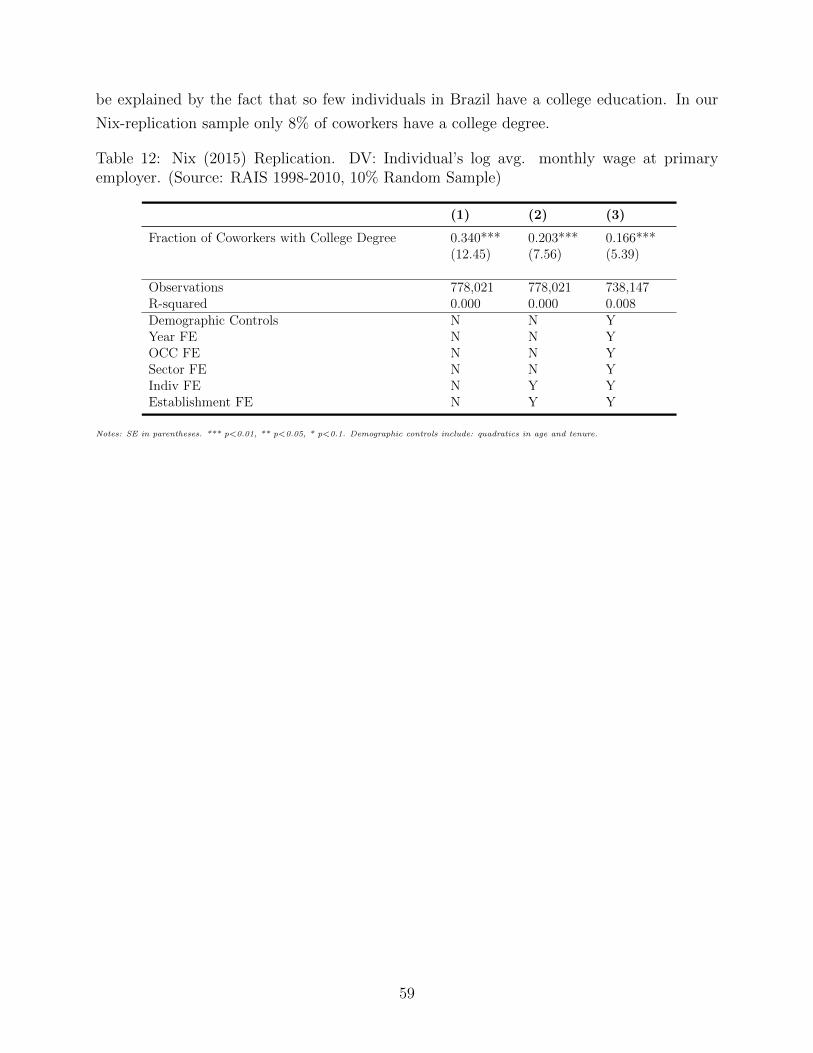
be explained by the fact that so few individuals in Brazil have a college education. In our

Nix-replication sample only 8% of coworkers have a college degree.

Table 12: Nix (2015) Replication. DV: Individual’s log avg. monthly wage at primaryemployer. (Source: RAIS 1998-2010, 10% Random Sample)

(1) (2) (3)

Fraction of Coworkers with College Degree 0.340*** 0.203*** 0.166***(12.45) (7.56) (5.39)

Observations 778,021 778,021 738,147R-squared 0.000 0.000 0.008Demographic Controls N N YYear FE N N YOCC FE N N YSector FE N N YIndiv FE N Y YEstablishment FE N Y Y

Notes: SE in parentheses. *** p<0.01, ** p<0.05, * p<0.1. Demographic controls include: quadratics in age and tenure.

59

References

John M Abowd, Francis Kramarz, and David N Margolis. High wage workers and high wage

firms. Econometrica, 67(2):251–333, 1999.

Axel Anderson. A dynamic generalization of becker’s assortative matching result. Journal

of Economic Theory, 159:290–310, 2015.

Axel Anderson and Lones Smith. Dynamic matching and evolving reputations. The Review

of Economic Studies, 77(1):3–29, 2010.

Ana Luisa Pessoa Araujo. Wage inequality and job stability. 2014.

Tania Babina. Destructive creation at work: How financial distress spurs entrepreneurship.

2015.

Stephane Bonhomme, Thibaut Lamadon, and Elena Manresa. A distributional framework

for matched employer employee data. 2014.

Katarna Borovickova and Robert Shimer. High wage workers work for high wage firms.

Manuscript, 2017.

Wyatt Brooks, Kevin Donovan, and Terence R Johnson. Mentors or teachers? microenter-

prise training in kenya. Manuscript, 2017.

Martin Browning and Thomas F Crossley. Unemployment insurance benefit levels and con-

sumption changes. Journal of Public Economics, 80(1):1–23, 2001.

Francisco J Buera and Ezra Oberfield. The global diffusion of ideas. Technical report,

National Bureau of Economic Research, 2016.

Pierre Cahuc, Fabien Postel-Vinay, and Jean-Marc Robin. Wage bargaining with on-the-job

search: Theory and evidence. Econometrica, 74(2):323–364, 2006.

Hector Chade and Jan Eeckhout. Stochastic sorting. In 2013 Meeting Papers, number 1222.

Society for Economic Dynamics, 2013.

Hector Chade, Jan Eeckhout, and Lones Smith. Sorting through search and matching models

in economics. Journal of Economic Literature, 55(2):493–544, 2017.

Satyajit Chatterjee and Esteban Rossi-Hansberg. Spinoffs and the market for ideas. Inter-

national Economic Review, 53(1):53–93, 2012.

60

Jonathan Chiu, Cesaire Meh, and Randall Wright. Innovation and growth with financial,

and other, frictions. International Economic Review, 58(1):95–125, 2017.

Thomas Cornelissen, Christian Dustmann, and Uta Schonberg. Peer effects in the workplace.

American Economic Review, 2016.

Jan Eeckhout and Boyan Jovanovic. Knowledge spillovers and inequality. American Eco-

nomic Review, 92(5):1290–1307, 2002.

Niklas Engbom and Christian Moser. Earnings inequality and the minimum wage: Evidence

from brazil. 2016.

Fatih Guvenen, Fatih Karahan, Serdar Ozkan, and Jae Song. What do data on millions

of us workers reveal about life-cycle earnings risk? Technical report, National Bureau of

Economic Research, 2015.

Marcus Hagedorn, Tzuo Hann Law, and Iourii Manovskii. Identifying equilibrium models of

labor market sorting. Technical report, National Bureau of Economic Research, 2012.

Tom-Reiel Heggedal, Espen R Moen, and Edgar Preugschat. Productivity spillovers through

labor mobility in search equilibrium. Journal of Economic Theory, 169:551–602, 2017.

Kyle Herkenhoff, Gordon Phillips, and Ethan Cohen-Cole. How credit constraints impact job

finding rates, sorting & aggregate output. Technical report, National Bureau of Economic

Research, 2016.

Boyan Jovanovic. Misallocation and growth. American Economic Review, 104(4):1149–71,

2014.

Boyan Jovanovic and Rafael Rob. The growth and diffusion of knowledge. The Review of

Economic Studies, 56(4):569–582, 1989.

Rasmus Lentz and Nicolas Roys. Training and search on the job. Technical report, National

Bureau of Economic Research, 2015.

Jeremy Lise and Fabien Postel-Vinay. Multidimensional skills, sorting, and human capital

accumulation. (Working Paper), 2015.

Robert E Lucas and Benjamin Moll. Knowledge growth and the allocation of time. Journal

of Political Economy, 122(1):1–51, 2014.

61

Erzo G.J. Luttmer. An assignment model of knowledge diffusion and income inequality.

Federal Reserve Bank of Minneapolis Research Department Staff Report, 715, 2014.

Alexandre Mas and Enrico Moretti. Peers at work. The American economic review, 99(1):

112–145, 2009.

Alexander Monge-Naranjo. Foreign firms and the diffusion of knowledge. 2012.

Marc-Andreas Muendler, Jennifer Poole, Garey Ramey, and Tamara Wajnberg. Job con-

cordances for brazil: Mapping the classificacao brasileira de ocupacoes (cbo) to the in-

ternational standard classification of occupations (isco-88). University of California, San

Diego, unpublished manuscript, 2004.

Emily Nix. Learning spillovers in the firm. Technical report, mimeo, 2015.

Jesse Perla and Christopher Tonetti. Equilibrium imitation and growth. Journal of Political

Economy, 122(1):52–76, 2014.

Fabien Postel-Vinay and Jean-Marc Robin. Equilibrium wage dispersion with worker and

employer heterogeneity. Econometrica, 70(6):2295–2350, 2002.

Michel Serafinelli. Good firms, worker flows and local productivity. Technical report, Uni-

versity of Toronto, Department of Economics, 2015.

Robert Shimer and Lones Smith. Assortative matching and search. Econometrica, 68(2):

343–369, 2000.

James R Spletzer. Inequality statistics from the lehd. In June 2014 FESAC meetings,

http://www. census. gov/fesac/pdf/2014-06-13/Spletzer Background. pdf, 2014.

Andrey Stoyanov and Nikolay Zubanov. Productivity spillovers across firms through worker

mobility. American Economic Journal: Applied Economics, 4(2):168–98, 2012.

62