Knowledge Capital and U.S. State-level Differences in ...

Knowledge Capital and U.S. State-level Differences in Labor Productivity

Sabrina Wulff Pabilonia, Ph.D. U.S. Bureau of Labor Statistics

2 Massachusetts Ave., NE, Rm. 2180 Washington, DC 20212

Email: [email protected]

Susan Fleck, Ph.D. U.S. Bureau of Labor Statistics

2 Massachusetts Ave., NE, Rm. 3955 Washington, DC 20212

Email: [email protected]

Initial Draft: August 2018 This Draft: December 2019

Abstract: Hanushek, Ruhose, and Woessmann used income measures to analyze the impact

of knowledge capital on state-level economic development. Recently published experimental state-level labor productivity measures from the U.S. Bureau of Labor Statistics provide the opportunity to extend their analysis to labor productivity. We find that in 2017, 12 percent of the dispersion in labor productivity levels is attributable to variation in knowledge capital. We also find that over the post-Great Recession period (2009–2017), initial knowledge capital is positively correlated with productivity growth: increasing test scores by one standard deviation is associated with a 1.6-percentage-point-faster average annual productivity growth rate.

JEL codes: I25, I26, J24, R11, R23

Keywords: state productivity, knowledge capital, human capital

Acknowledgements: All views expressed in this paper are those of the authors and do not necessarily reflect the views or policies of the U.S. Bureau of Labor Statistics. We thank Lucy Eldridge, Barbara Fraumeni, Robert Hill, Mike Jadoo, Charlene Kalenkoski, Bhavani Khandrika, Peter Meyer, Jennifer Price, Jay Stewart, Bryan Stuart, and participants at the 2018 International Association for Research in Income and Wealth General Conference, 2018 Southern Economic Association Meetings, and Society of Government Economists Annual Meeting for useful input and comments.

1

I. Introduction

Human capital is an important input in economic growth. Most prior research on the

contribution of human capital to cross-state or cross-country differences in growth has used years

of schooling as a measure of workers’ skills, yet skills clearly encompass more than schooling

attainment. Recently, Hanushek, Ruhose, and Woesmann (2017b) (hereafter HRW) developed a

detailed measure of state-level knowledge capital using a combination of years of schooling and

achievement test scores to capture both the quantity and quality of skill investments. Their

measure accounts for state-level skill differences resulting from differences in families, innate

abilities, health, the quality of schools, etc. for state residents who remain in their state of birth as

well as the skills for those who migrate from other states or countries.

HRW apply this knowledge capital measure in a development accounting framework to

explain state-level GDP per capita differences. They present a model based on an aggregate

Cobb-Douglas production function and use GDP per capita as their measure of labor

productivity. Whereas GDP per capita better measures income, GDP per hour worked is by far a

better measure of labor productivity. GDP per capita is influenced by fertility and mortality rates,

the number of hours worked, labor force participation, and employment rates (Santacreu 2015).

In a cross-country analysis, Santacreu (2015) shows that there are large differences in the relative

position of countries to the United States when using GDP per capita instead of GDP per hour

worked. The decomposition of GDP per capita for the total economy displayed below shows

how labor productivity is related to GDP per capita:

𝐺𝐺𝐺𝐺𝐺𝐺𝐺𝐺𝑃𝑃𝑃𝑃𝑃𝑃𝑃𝑃𝑃𝑃𝑃𝑃𝑃𝑃𝑃𝑃𝑃𝑃

= 𝐺𝐺𝐺𝐺𝐺𝐺

𝐻𝐻𝑃𝑃𝑃𝑃𝐻𝐻𝐻𝐻 𝑤𝑤𝑃𝑃𝐻𝐻𝑤𝑤𝑤𝑤𝑤𝑤∗

𝐻𝐻𝑃𝑃𝑃𝑃𝐻𝐻𝐻𝐻 𝑤𝑤𝑃𝑃𝐻𝐻𝑤𝑤𝑤𝑤𝑤𝑤𝐸𝐸𝐸𝐸𝑃𝑃𝑃𝑃𝑃𝑃𝐸𝐸𝑤𝑤𝑤𝑤 𝑃𝑃𝑤𝑤𝐻𝐻𝐻𝐻𝑃𝑃𝑃𝑃𝐻𝐻

∗𝐸𝐸𝐸𝐸𝑃𝑃𝑃𝑃𝑃𝑃𝐸𝐸𝑤𝑤𝑤𝑤 𝑃𝑃𝑤𝑤𝐻𝐻𝐻𝐻𝑃𝑃𝑃𝑃𝐻𝐻

𝐺𝐺𝑃𝑃𝑃𝑃𝑃𝑃𝑃𝑃𝑃𝑃𝑃𝑃𝑃𝑃𝑃𝑃𝑃𝑃 (1)

Of the three terms on the right-hand side of the equation, the first term — labor productivity —

captures technological change, capital deepening and labor composition; the second term —

2

hours worked per employed person — captures effort, and the final term — the employment-to-

population ratio — reflects both labor force participation and employment rates. It is primarily

through the effect of knowledge skills on the labor productivity term that we expect to see

changes in knowledge skills impacting GDP per capita.

The current paper examines the contribution of knowledge capital to state-level labor

productivity differences. We do so by replacing the outcome variable in HRW’s model, GDP per

capita, with a recently released experimental state-level labor productivity measure by the U.S.

Bureau of Labor Statistics (BLS (2019).1 While HRW’s analyses are based on GDP per capita

for the total economy, the new BLS output per hour worked data series cover the private

nonfarm sector (PNF) and align with official U.S. national-level productivity measures.2 The

state-level output series is constructed using the U.S. Bureau of Economic Analysis’s (BEA)

GDP by state and detailed industry measures. The state-level hours worked series is constructed

following the methodology for BLS national-level productivity measures to the extent possible

with the state-level hours data available.3 The new BLS hours worked series begins in 2007, the

year HRW’s analysis ended. Thus, our analysis begins in 2007 for comparison purposes. We

then provide development accounting estimates for more recent years and examine the

1 This experimental data set can be found at: https://www.bls.gov/lpc/state-productivity.htm. 2 The nonfarm business sector labor productivity measure is a principal federal economic indicator. The experimental state-level data series has slightly different sectoral coverage because it 1) excludes government enterprises and 2) includes nonprofits serving households. Nevertheless, the official U.S measures and sum-of-states measures trend closely (Pabilonia et al. 2019). National productivity measures exclude the general government sector and nonprofits because output measures for these sectors are measured using compensation. Thus, both output and hours for these sectors will trend similarly. The inclusion of these sectors in productivity measures may bias productivity estimates toward zero. Agricultural hours are also difficult to measure at the state level. 3 The hours methodology for national estimates can be found at: https://www.bls.gov/lpc/lprswawhtech.pdf (U.S. Bureau of Labor Statistics 2004).

3

relationship between knowledge capital in 2009 and the growth in output per hour worked over

the post-Great Recession period (2009–2017). Given that our new measure is not a total

economy measure, we slightly modify equation 1 and add two additional terms, a

government/agriculture effect and a private nonfarm sector employment share, in order to show

how GDP per capita is related to output per hour worked in the private nonfarm sector as shown

below in equation 2:

𝐺𝐺𝐺𝐺𝐺𝐺𝐺𝐺𝑃𝑃𝑃𝑃𝑃𝑃𝑃𝑃𝑃𝑃𝑃𝑃𝑃𝑃𝑃𝑃𝑃𝑃


𝑂𝑂𝑃𝑃𝑃𝑃𝑃𝑃𝑃𝑃𝑃𝑃𝑃𝑃𝑃𝑃𝑃𝑃∗

𝑂𝑂𝑃𝑃𝑃𝑃𝑃𝑃𝑃𝑃𝑃𝑃𝑃𝑃𝑃𝑃𝑃𝑃𝐻𝐻𝑃𝑃𝑃𝑃𝐻𝐻𝐻𝐻 𝑤𝑤𝑃𝑃𝐻𝐻𝑤𝑤𝑤𝑤𝑤𝑤𝑃𝑃𝑃𝑃𝑃𝑃

∗𝐻𝐻𝑃𝑃𝑃𝑃𝐻𝐻𝐻𝐻 𝑤𝑤𝑃𝑃𝐻𝐻𝑤𝑤𝑤𝑤𝑤𝑤𝑃𝑃𝑃𝑃𝑃𝑃

𝐸𝐸𝐸𝐸𝑃𝑃𝑃𝑃𝑃𝑃𝐸𝐸𝑤𝑤𝑤𝑤 𝑃𝑃𝑤𝑤𝐻𝐻𝐻𝐻𝑃𝑃𝑃𝑃𝐻𝐻𝑃𝑃𝑃𝑃𝑃𝑃

∗𝐸𝐸𝐸𝐸𝑃𝑃𝑃𝑃𝑃𝑃𝐸𝐸𝑤𝑤𝑤𝑤 𝑃𝑃𝑤𝑤𝐻𝐻𝐻𝐻𝑃𝑃𝑃𝑃𝐻𝐻𝑃𝑃𝑃𝑃𝑃𝑃𝐸𝐸𝐸𝐸𝑃𝑃𝑃𝑃𝑃𝑃𝐸𝐸𝑤𝑤𝑤𝑤 𝑃𝑃𝑤𝑤𝐻𝐻𝐻𝐻𝑃𝑃𝑃𝑃𝐻𝐻


𝐺𝐺𝑃𝑃𝑃𝑃𝑃𝑃𝑃𝑃𝑃𝑃𝑃𝑃𝑃𝑃𝑃𝑃𝑃𝑃 (2)

We find that 10–16 percent of the dispersion in the 2007 state productivity levels and 12

percent of the dispersion in the 2017 state productivity levels is attributable to state-level

variation in knowledge capital. In 2009, knowledge capital explained 8 percent of the dispersion.

In each instance, test scores contribute slightly more than years of schooling to explaining level

differences in state productivity. Over the period 2009–2017, we find a positive relationship

between knowledge capital in 2009 and productivity growth, which can be explained by

differences in state average test scores rather than years of schooling.

Section II describes the state-level labor productivity and knowledge capital measures used.

Section III uses these measures in a developmental accounting framework. Section IV presents

the results from growth regression models that incorporate knowledge capital. Section V

concludes.

II. Data

A. State Labor Productivity

4

Most prior research on state-level labor productivity has used either total population or the

number of employed persons as the labor input whereas this study uses hours worked as the labor

input. Hours worked is the preferable labor input, because it measures time available for

production. In 2007, the BLS began publishing state-level all-employee average weekly hours

paid using data from its establishment survey, the Current Employment Statistics (CES); hours

from a business survey in theory count the hours worked in the state where the production takes

place rather than the place of residence. This new measure made it possible for BLS to construct

the experimental output per hour series where output and hours measures have the same

geographic coverage. Hours paid are converted to hours worked using information on paid leave

from the National Compensation Survey. Hours worked include those worked by wage and

salary workers, unincorporated self-employed workers, and unpaid family workers.

The private nonfarm output measure used in this paper is a real output series constructed

from the all-private industries output measure in the BEA’s GDP by state accounts and removing

output for the farm sector, private households and owner-occupied housing. Although state

prices differ, there are currently no state-level price deflators, so national-level industry price

deflators are used. The base year for real output is 2012. Productivity measured in levels is

constructed as real output divided by hours worked. Productivity growth is the percentage

growth in output minus the percentage growth in hours worked. For more details on the

methodology and construction of the new measure, see Pabilonia et al. (2019).

For comparison’s sake in the developmental accounting analyses, we first calculate results

using the same 47 states considered by HRW. HRW excluded Alaska and Wyoming, where over

27 percent of GDP resulted from extraction activities in 2007; they excluded Delaware because

Delaware is a tax haven for many companies, and finance and insurance accounted for over 35

5

percent of that state’s GDP in 2007. They also exclude the District of Columbia, because it is

difficult to measure the District’s knowledge and physical capital. All other estimates in the

paper are based upon all 50 states.

Summary statistics for the data used in this paper are presented in Table 1. We compare our

findings in 2007 with HRW’s results using GDP per capita. We also estimate models using

productivity data for 2009 and 2017. Figure 1 highlights the dispersion in productivity levels

across states. Between 2007 and 2017, the mean output per hour worked rose from $55.24 to

$60.48. Dispersion across states (as measured by the standard deviation) fell slightly from $10.57

to $10.44 over the same time period. Using an alternative measure of dispersion – the

interquartile range, we find that the state at the 75th percentile of the productivity distribution was

1.19 times more productive than the state at the 25th percentile in 2007, but 1.23 times more

productive in 2017.

B. State Knowledge Capital

We next briefly summarize the state knowledge capital measures, which were developed by

HRW (2017b). Using a Mincer-type earnings function, HRW augment school attainment with

test scores to create a measure of aggregate knowledge capital per worker. Specifically,

knowledge capital h is represented as

ℎ = 𝑤𝑤𝑟𝑟𝑟𝑟+𝑤𝑤𝑤𝑤 (3)

where S is the average years of schooling in a state for the non-enrolled working age population

aged 20–65, T is the average test score for a state’s working age population aged 20–65, r is the

earnings gradient for years of schooling (assumed to be equal to 0.08), and w is the earnings

gradient for test scores (assumed to be equal to 0.17). These gradient values are based upon the

findings from micro-economic literature. For example, Hanushek et al. (2015) and Hanushek and

Zhang (2009) both find r = 0.08 using recent U.S. data and estimating returns across the

6

lifecycle. Hanushek and Zhang (2009) find w = 0.193 using the International Adult Literacy

Survey (IALS), while Hanushek et al. (2015) find w = 0.138 using the 2012 Programme for the

International Assessment of Adult Competencies (PIAAC). In both instances, they estimate the

returns to skills across the lifecycle, although they use tests given at the time earnings are

observed rather than during earlier schooling. In an additional analysis to account for the effects

of skill-biased technological change, HRW allow r to vary based upon the average years of

schooling at the tertiary and non-tertiary levels, where the former is set to 0.157 and the latter is

set to 0.057 based upon results from a standard Mincer wage regression using the 2007 IPUMS

data.

HRW calculate average years of schooling in a state for the working-age population aged 20-

65 not currently enrolled in school using the highest years of schooling completed reported in the

American Community Survey (ACS). We first follow HRW’s data restrictions but then also

calculate years of schooling for the entire working-age population aged 20–65, because we are

interested in the relationship between knowledge capital available for production and

productivity growth, which is important when we examine productivity growth over the post-

recessionary period. In addition, many students work while enrolled in school. We follow

HRW’s methodology for constructing years of schooling by converting degree attainment

reported in the ACS to years of schooling following Jaeger (1999) and assigning GED holders 10

years of schooling.4 Figure 2 shows the distribution of mean years of schooling across states.

The average of the state average years of schooling increases slightly from 13.17 in 2007 to

4 We use the IPUMS-USA data (Ruggles et al. 2019). GED holders are assigned 10 years of schooling because they tend to have relatively weak labor market performance (Heckman, Humphries, and Mader 2011).

7

13.40 in 2017 (Table 1) and, for each state, the average years of schooling in 2017 are greater

than or equal to the average years of schooling in 2007 (see Appendix Table A1).

HRW’s preferred test score measures, which we use here without modification, are based

primarily upon eighth grade mathematics achievement test scores from the National Assessment

of Educational Progress (NAEP) from 1978 to 1992 at the national level and 1992 through 2011

at the state level. State test scores are initially normalized to have a U.S. mean of 500 and

standard deviation of 100 in the year 2011. Their measures account for both selective migration

and heterogeneous fertility. They impute test scores for individual observations in the ACS based

upon state identifiers and educational attainment (university degree or not). Furthermore, HRW

combine data from international achievement tests with population shares of international

migrants based upon their country of origin to adjust for selective migration. They then backcast

state scores from 1978 to 1992 using national trends to obtain the skills of the current working-

age population. HRW’s 2012 test score measures, the latest available, are used as a proxy for the

2017 test scores in the analyses.5 See HRW (2017b) for more details on the construction of the

test score measures and Appendix Table A1 for the schooling data used in this paper.

III. Development Accounting Framework

One goal of this paper is to determine the extent to which productivity-level differences

across U.S. states can be accounted for by state-level knowledge capital differences. Figures 3–8

show scatterplots of the association between log output per hour worked and the schooling

measures in 2007, 2009, and 2017. In 2007, the cross-state correlations are 0.227 between log

5 HRW’s 2012 measures incorporate two additional years of data beyond 2007. Given time constraints and the complexity of replicating their measures, we make the assumption that the 2012 test score measures approximate the 2017 measures if they were to be constructed.

8

output per hour worked and mean years of schooling and 0.216 between log output per hour

worked and test scores (Table 2). These correlations are significantly lower than the correlations

of the knowledge capital components with log GDP per capita in 2007 (0.464 and 0.470

respectively). We note that the correlation between log GDP per capita and log output per hour

worked is 0.882 in 2007. In 2009, the cross-state correlations are 0.266 between log output per

hour worked and mean years of schooling and 0.208 between log output per hour worked and

test scores (Table 3). In 2017, the cross-state correlations are 0.313 between log output per hour

worked and mean years of schooling and 0.339 between log output per hour worked and test

scores (Table 3).

We apply HRW’s development accounting framework in order to provide an indication of

the causal contributions of knowledge capital to labor productivity. This framework is based

upon the following aggregate Cobb-Douglas production function:

𝑌𝑌 = (ℎ𝐿𝐿)1−𝛼𝛼𝐾𝐾𝛼𝛼𝐴𝐴𝜆𝜆 (4)

where Y is output; L is labor input measured as hours worked; h is aggregate knowledge capital

per worker; K is physical capital stock; and 𝐴𝐴𝜆𝜆 represents multi-factor productivity. Assuming

𝜆𝜆 = 1 − 𝛼𝛼 (i.e. Harrod-neutral productivity), then labor productivity, y, can be written as:

𝑌𝑌𝐿𝐿≡ 𝐸𝐸 = ℎ �𝑘𝑘

𝑦𝑦�𝛼𝛼

(1−𝛼𝛼)�𝐴𝐴, (5)

where 𝑤𝑤 ≡ 𝐾𝐾𝐿𝐿 is the capital-labor ratio.

After taking logarithms, we can write the decomposition of the variations in labor

productivity as

𝑣𝑣𝑃𝑃𝐻𝐻(𝑃𝑃𝑃𝑃(𝐸𝐸)) = 𝑐𝑐𝑃𝑃𝑣𝑣(𝑃𝑃𝑃𝑃(𝐸𝐸) , 𝑃𝑃𝑃𝑃(ℎ)) + 𝑐𝑐𝑃𝑃𝑣𝑣 �𝑃𝑃𝑃𝑃(𝐸𝐸) , 𝑃𝑃𝑃𝑃 ��𝑘𝑘𝑦𝑦�𝛼𝛼

(1−𝛼𝛼)�� + 𝑐𝑐𝑃𝑃𝑣𝑣(𝑃𝑃𝑃𝑃(𝐸𝐸) , 𝑃𝑃𝑃𝑃(𝐴𝐴)). (6)

9

We then divide each term in equation 5 by the variance in state-level labor productivity in

order to put each component in terms of its proportional contribution to the variance in state-

level labor productivity:

𝑐𝑐𝑐𝑐𝑐𝑐(𝑙𝑙𝑙𝑙(𝑦𝑦),𝑙𝑙𝑙𝑙(ℎ))𝑐𝑐𝑣𝑣𝑟𝑟(𝑙𝑙𝑙𝑙(𝑦𝑦))

+ 𝑐𝑐𝑐𝑐𝑐𝑐�𝑙𝑙𝑙𝑙(𝑦𝑦),𝑙𝑙𝑙𝑙��𝑘𝑘𝑦𝑦�

𝛼𝛼(1−𝛼𝛼)�

��

𝑐𝑐𝑣𝑣𝑟𝑟(𝑙𝑙𝑙𝑙(𝑦𝑦))+ 𝑐𝑐𝑐𝑐𝑐𝑐(𝑙𝑙𝑙𝑙(𝑦𝑦),𝑙𝑙𝑙𝑙(𝐴𝐴))

𝑐𝑐𝑣𝑣𝑟𝑟(𝑙𝑙𝑙𝑙(𝑦𝑦))= 1. (7)

We estimate only the first covariance term of the decomposition, the contribution of knowledge

capital to the variance in labor productivity, in equation 7.6 Results using our state-level labor

productivity measure, private nonfarm output per hour worked, compared to HRW’s GDP per

capita measure are presented in Table 4.

We find that in 2007 using HRW sample restrictions, 10 percent of the dispersion in state-

level labor productivity results from differences in knowledge capital, with 6 percent coming

from differences in test scores and 4 percent coming from differences in years of schooling (row

2). This is low compared to HRW (row 1), who find that 23 percent of the variation in GDP per

capita in the same year is explained by differences in knowledge capital. To explain the

difference, we can write out an additional covariance decomposition of equation 2. For

simplicity of exposition, we rename the terms in equation 2 as y0-y5:

𝐺𝐺𝐺𝐺𝐺𝐺𝐺𝐺𝑃𝑃𝑃𝑃𝑃𝑃𝑃𝑃𝑃𝑃𝑃𝑃𝑃𝑃𝑃𝑃𝑃𝑃��

𝑦𝑦0


𝑂𝑂𝑃𝑃𝑃𝑃𝑃𝑃𝑃𝑃𝑃𝑃𝑃𝑃𝑃𝑃𝑃𝑃��𝑦𝑦1

∗𝑂𝑂𝑃𝑃𝑃𝑃𝑃𝑃𝑃𝑃𝑃𝑃𝑃𝑃𝑃𝑃𝑃𝑃

𝐻𝐻𝑃𝑃𝑃𝑃𝐻𝐻𝐻𝐻 𝑤𝑤𝑃𝑃𝐻𝐻𝑤𝑤𝑤𝑤𝑤𝑤𝑃𝑃𝑃𝑃𝑃𝑃��𝑦𝑦2

∗𝐻𝐻𝑃𝑃𝑃𝑃𝐻𝐻𝐻𝐻 𝑤𝑤𝑃𝑃𝐻𝐻𝑤𝑤𝑤𝑤𝑤𝑤𝑃𝑃𝑃𝑃𝑃𝑃

𝐸𝐸𝐸𝐸𝑃𝑃𝑃𝑃𝑃𝑃𝐸𝐸𝑤𝑤𝑤𝑤 𝑃𝑃𝑤𝑤𝐻𝐻𝐻𝐻𝑃𝑃𝑃𝑃𝐻𝐻𝑃𝑃𝑃𝑃𝑃𝑃��𝑦𝑦3

∗𝐸𝐸𝐸𝐸𝑃𝑃𝑃𝑃𝑃𝑃𝐸𝐸𝑤𝑤𝑤𝑤 𝑃𝑃𝑤𝑤𝐻𝐻𝐻𝐻𝑃𝑃𝑃𝑃𝐻𝐻𝑃𝑃𝑃𝑃𝑃𝑃𝐸𝐸𝐸𝐸𝑃𝑃𝑃𝑃𝑃𝑃𝐸𝐸𝑤𝑤𝑤𝑤 𝑃𝑃𝑤𝑤𝐻𝐻𝐻𝐻𝑃𝑃𝑃𝑃𝐻𝐻��

𝑦𝑦4


𝐺𝐺𝑃𝑃𝑃𝑃𝑃𝑃𝑃𝑃𝑃𝑃𝑃𝑃𝑃𝑃𝑃𝑃𝑃𝑃��𝑦𝑦5

6 Even though A can be endogenous, Klenow and Rodríquez-Clare (1997) conclude that it is still useful to examine this decomposition because education policies can affect h more than other factors. Therefore, finding that high levels of labor productivity are explained mostly by high levels of h would suggest that differences in education policies are important for explaining state-level differences in labor productivity.

10

The covariance decomposition is then:

𝑐𝑐𝑃𝑃𝑣𝑣(𝑃𝑃𝑃𝑃𝐸𝐸0, 𝑃𝑃𝑃𝑃ℎ)𝑣𝑣𝑃𝑃𝐻𝐻(𝑃𝑃𝑃𝑃𝐸𝐸0)

= 𝑣𝑣𝑃𝑃𝐻𝐻(𝑃𝑃𝑃𝑃𝐸𝐸1)𝑣𝑣𝑃𝑃𝐻𝐻(𝑃𝑃𝑃𝑃𝐸𝐸0)


+ 𝑣𝑣𝑃𝑃𝐻𝐻(𝑃𝑃𝑃𝑃𝐸𝐸2)𝑣𝑣𝑃𝑃𝐻𝐻(𝑃𝑃𝑃𝑃𝐸𝐸0)








(8)

The first term on the left 𝑐𝑐𝑐𝑐𝑐𝑐(𝑙𝑙𝑙𝑙𝑦𝑦0,𝑙𝑙𝑙𝑙ℎ)𝑐𝑐𝑣𝑣𝑟𝑟(𝑙𝑙𝑙𝑙𝑦𝑦0)

is what HRW (2017b) estimate while we estimate

𝑐𝑐𝑐𝑐𝑐𝑐(𝑙𝑙𝑙𝑙𝑦𝑦2,𝑙𝑙𝑙𝑙ℎ)𝑐𝑐𝑣𝑣𝑟𝑟(𝑙𝑙𝑙𝑙𝑦𝑦2)

. In Table 5, we present estimates for the terms in the decomposition for the year

2007 using the latest state GDP per capita measures from BEA, updated in November 2019 (U.S.

Bureau of Economic Analysis 2019). The first covariance (row 1) is very close to the estimate in

HRW (2017b) (0.224 versus 0.228). We find that the contribution of knowledge capital to the

variance in GDP per capita can also be explained to a great extent by the contribution of

knowledge capital to the variance in the employment-to-population ratio (row 11). Interestingly,

the contribution of knowledge capital to the variance in state hours per worker is negative,

indicating they vary in opposite directions.

We next loosen the sample restrictions and extend the analysis to 2017. In row 3 of Table 4,

we expand the sample to include all 50 states. In this sample, only 8 percent of the dispersion in

state-level labor productivity results from differences in knowledge capital, with slightly more

explained by test scores than years of schooling. In 2009 at the trough of the current business

cycle, we find that knowledge capital explains 8 percent of the dispersion in labor productivity.

In row 5, we show that including those enrolled in schooling barely changes our estimates. In

2017, 12 percent of the dispersion in state productivity results from differences in knowledge

11

capital, with 7 percent coming from differences in test scores and 5 percent coming from

differences in years of schooling.

We then compare 2007 estimates where we allow the returns on years of schooling to differ

for tertiary and non-tertiary schooling (rows 7 and 8). HRW (2017b) found that knowledge

capital explains 31 percent of the dispersion in GDP per capita. We find that knowledge capital

explains only 16 percent of the dispersion in labor productivity, with the differences in years of

schooling explaining almost double the differences in test scores (10 percent versus 6 percent).

Next we examine the contribution of knowledge capital to the average log difference in labor

productivity between the top five and bottom five states in the productivity distribution using the

production function (equation 5). The five-state measure below shows the proportional

contribution of the factors and total factor productivity to the average log difference in the top

five and bottom five states:

ln [(Π𝑖𝑖=15 ℎ𝑖𝑖 Π𝑗𝑗=𝑛𝑛−4

𝑛𝑛 ℎ𝑗𝑗� )1/5]

ln [(Π𝑖𝑖=15 𝑦𝑦𝑖𝑖 Π𝑗𝑗=𝑛𝑛−4

𝑛𝑛 𝑦𝑦𝑗𝑗� )1/5]+ ln [(Π𝑖𝑖=1

5 𝑘𝑘𝑖𝑖 Π𝑗𝑗=𝑛𝑛−4𝑛𝑛 𝑘𝑘𝑗𝑗� )1/5]


𝑛𝑛 𝑦𝑦𝑗𝑗� )1/5] + ln [(Π𝑖𝑖=1

5 𝐴𝐴𝑖𝑖 Π𝑗𝑗=𝑛𝑛−4𝑛𝑛 𝐴𝐴𝑗𝑗� )1/5]


𝑛𝑛 𝑦𝑦𝑗𝑗� )1/5] = 1, (9)

where i and j are states ranked according to their output per hour worked, i,…,j,…,n, among the

total of n states.7 The five-state knowledge capital measure, which we estimate, is the first term

in equation 7.

Comparing our results to HRW’s with the same knowledge capital measure for 2007, we

find that the five-state knowledge capital measure accounts for only 5 percent of the difference in

7 In 2007, the top five most productive states of the 47 states HRW examined are Connecticut, New York, New Jersey, Louisiana, and Massachusetts. The least productive states in 2007 are Mississippi, Montana, Maine, Vermont, and Idaho. This ranking differs from the GDP per capita ranking, especially for the least productive states. In 2017, the ranking changed so the top five most productive states are New York, Connecticut, California, Washington, and Massachusetts. The least productive states in 2017 are Arkansas, Vermont, Idaho, Mississippi, and Maine.

12

labor productivity in contrast to 31 percent of the difference in GDP per capita (Table 4). For the

same year, test scores and years of schooling contribute equally to the difference; in the HRW

specification, test scores contribute 55 percent more than years of schooling (19 percent and 12

percent respectively). In 2017, we find that the five-state knowledge capital measure accounts for

10 percent of the difference in labor productivity, but test scores are much more important than

years of schooling (7 percent and 3 percent).

IV. Growth Regression Models

We next examine cross-state differences in labor productivity growth over the post-recession

period (2009–2017). Over this period, the official nonfarm business sector labor productivity

grew on an average annual basis by 0.93 percent. However, we find considerable heterogeneity

across states, with a standard deviation in the growth rate of 0.70 percent and range of 3.7

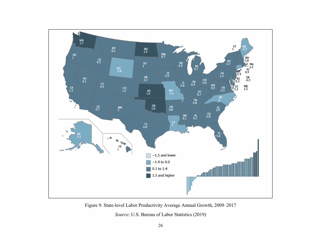
percentage points (Figure 9; Table 1).

Motivated by Hanushek, Ruhose, Woessmann (2017a) (hereafter HRW (2017a)), we

estimate the following productivity growth model that incorporates test scores:

%𝛥𝛥𝐸𝐸𝑠𝑠 = 𝛼𝛼 + 𝛽𝛽1𝑇𝑇𝑠𝑠 + 𝛽𝛽2𝑆𝑆𝑠𝑠 + 𝑋𝑋𝑠𝑠𝛿𝛿 + 𝜀𝜀𝑠𝑠 (10)

where %𝛥𝛥𝐸𝐸𝑠𝑠 is the average annual growth rate in labor productivity in state s between 2009 and

2017, 𝑇𝑇𝑠𝑠 is the average test scores of the working-age population in state s divided by 100 (the

standard deviation) in 2009, 𝑆𝑆𝑠𝑠 is the average years of schooling of the working-age population

in state s in 2009, 𝑋𝑋𝑠𝑠 is a matrix of state-level control variables all measured in 2009 including

the log of initial level of output per hour, the log of physical capital stock per worker, the log of

population density, the percent of each NAICS supersector output in private nonfarm output (the

13

percent manufacturing is omitted), and Census region fixed effects, and 𝜀𝜀𝑠𝑠 is an error term.8 This

analysis is descriptive and not meant to establish causality. However, numerous cross-country

analyses have established that greater knowledge capital leads to greater economic growth

(Hanushek and Woessmann 2012, 2015) even when accounting for endogeneity bias.9

Table 6 presents estimates for five specifications of our productivity growth model to

examine the relationship between knowledge capital and labor productivity growth. The first

three specifications follow HRW, including state-level controls for log of initial level of output

per hour and the log of physical capital stock per worker. The first model uses years of schooling

as the human capital measure. The second model adds test scores as a cognitive skills measure.

The third model includes Census region fixed effects in order to account for differences that are

geographically correlated. In the fourth model, we add the additional state-level controls —

population density and state industrial structure. In the fifth model, the observations are weighted

by the state population in 2009 so that small states do not overly affect the estimates.

In the first specification, we find a statistically significant positive relationship between years

of schooling and productivity growth. In specification two, we find that test scores and

productivity growth have a statistically significant positive relationship, but years of schooling

and productivity growth do not. The R-squared value increases from 0.33 to 0.40 with the

8 The inclusion of these additional controls is motivated in part by Panda (2017). The 2009 capital stock per worker measure is constructed for the private nonfarm sector using methodology outlined by Garofalo and Yamarik (2002) and data from the U.S. Bureau of Economic Analysis (2018b; 2018c). The methodology assumes that each industry has the same capital-output ratio across all states. Capital is the sum of the capital in each industry weighted by the state industry output share. The state population density is from the U.S. Census Bureau (2018). The percent of each NAICS supersector output in private nonfarm output in 2009 is estimated using GDP by state data (U.S. Bureau of Economic Analysis 2018a). The state population data for 2009 was obtained from the U.S. Bureau of Economic Analysis (2019). 9 For example, faster growth could lead states to invest more in education, and higher-skilled migrants could move to high growth states (HRW 2017a).

14

addition of the test scores. In the third specification when we add Census region, the coefficient

on test scores increases from 1.2 to 1.8. In the fourth specification, the R-squared value increases

from 0.43 to 0.68 and we again find a statistically significant positive relationship between test

scores and productivity growth (𝛽𝛽1 = 1.9). In all specifications, we also find the traditional

negative relationship between the initial productivity level in 2009 and subsequent productivity

growth, which is consistent with the literature on state-level productivity convergence (Barro and

Sala-i-Martin 1992; Mankiw, Romer and Weil 1992). In other words, states that are initially

behind in levels grow faster. In addition, we find a positive relationship between population

density and productivity growth. In the final specification (column 5), where the observations are

population weighted, we again find a statistically significant positive relationship between test

scores and productivity growth (𝛽𝛽1 = 1.6) — a one-standard-deviation increase in test scores is

associated with a 1.6-percentage-point-faster average annual productivity growth since the Great

Recession.10

V. Conclusion

There is substantial variation in U.S state-level labor productivity levels and growth rates. In

this paper, we examine the contribution that state-level knowledge capital, a measure based on

not just schooling attainment but also skills, makes to these productivity differences. We

replicate models examined in HRW (2017a; 2017b) but replace their outcome variable, GDP per

capita, with a more refined measure of labor productivity, output per hour worked. Using a

development accounting framework, we find that about 12 percent of the dispersion in state

10 If the sample is restricted to the 47 states used in HRW (2017a; 2017b), 𝛽𝛽1 equals 1.2.

15

productivity in 2017 results from differences in knowledge capital, with 5 percent coming from

differences in years of schooling and 7 percent coming from differences in test scores. Over the

period 2009–2017, we also find a statistically significant positive relationship between test

scores and productivity growth. These findings validate previous research of the importance of

cognitive skills in explaining productivity.

16

References

Barro, Robert and Xavier Sala-i-Martin. 1992. “Convergence.” Journal of Political Economy 100 (2): 223–251.

Garofalo, Gasper A. and Steven Yamarik. 2002. “Regional Convergence: Evidence from a New State-by-State Capital Stock Series.” Review of Economics and Statistics 84 (2): 316–323.

Hanushek, Eric A., Jens Ruhose, and Ludger Woessman. 2017a. “Economic Gains from Educational Reform by US States.” Journal of Human Capital 11 (4): 447–486.

Hanushek, Eric A., Jens Ruhose, and Ludger Woessman. 2017b. “Knowledge Capital and Aggregate Income Differences: Development Accounting for US States.” American Economic Journal: Macroeconomics 9 (4): 184–224, https://doi.org/10.1257/mac.20160255

Hanushek, Eric A., Guido Schwerdt, Simon Wiederhold, and Ludger Woessmann. 2015. “Returns to Skills around the World: Evidence from PIAAC.” European Economic Review 73: 103–30. Hanushek, Eric A., and Ludger Woessmann. 2012. “Do Better Schools Lead to More Growth? Cognitive Skills, Economic Outcomes, and Causation.” Journal of Economic Growth 17 (4): 267–321.

Hanushek, Eric A., and Lei Zhang. 2009. “Quality-Consistent Estimates of International Schooling and Skill Gradients.” Journal of Human Capital 3 (2): 107–43. Heckman, James J., John Eric Humphries, and Nicholas S. Mader. 2011. “The GED.” In Handbook of the Economics of Education, Vol. 3, edited by Eric A. Hanushek, Stephen Machin, and Ludger Woessmann, 423–83. Amsterdam: North-Holland. Jaeger, David A. 1997. “Reconciling the Old and New Census Bureau Education Questions: Recommendations for Researchers.” Journal of Business and Economic Statistics 15 (3): 300–309.

Klenow, Peter J., and Andrés Rodríquez-Clare. 1997. “The Neoclassical Revival in Growth Economics: Has It Gone Too Far?” In NBER Macroeconomics Annual 1997, Vol. 12, edited by Ben S. Bernanke and Julio J. Rotemberg, 73–114. Cambridge: MIT Press. Mankiw, N. Gregory, David Romer, and David N. Weil. 1992. “A Contribution to the Empirics of Economic Growth.” Quarterly Journal of Economics 107 (2): 407–37. Pabilonia, Sabrina Wulff, Michael W. Jadoo, Bhavani Khandrika, Jennifer Price, and James D. Mildenberger. 2019. “BLS Publishes Experimental State-level Labor Productivity Measures.” Monthly Labor Review. Panda, Bibhudutta. 2017. “Schooling and Productivity Growth: Evidence from a Dual Growth Accounting Application to U.S. States.” Journal of Productivity Analysis 48: 193–221.

17

Ruggles, Steven, Katie Genadek, Ronald Goeken, Josiah Grover, and Matthew Sobek. 2019. IPUMS USA: Version 9.0. Minneapolis, MN: IPUMS, 2019. https://doi.org/10.18128/D010.V9.0

Santacreu, Ana Maria. 2015. “Measuring Labor Productivity: Technology and the Labor Supply.” Economic Synopses, Federal Reserve Bank of St. Louis.

U.S. Bureau of Economic Analysis. 2018a. “Regional Economic Accounts, GDP per State.” http://www.bea.gov/regional/downloadzip.cfm (Accessed March 11, 2018).

U.S. Bureau of Economic Analysis. 2018b. “Table 3.1ESI. Current-Cost Net Stock of Private Fixed Assets by Industry.” (Accessed March 21, 2019).

U.S. Bureau of Economic Analysis. 2018c. “Table 3.2ESI. Chain-Type Quantity Indexes for Net Stock of Private Fixed Assets by Industry.” (Accessed March 21, 2019).

U.S. Bureau of Economic Analysis. 2019. “Regional Economic Accounts, GDP per State.” http://www.bea.gov/regional/downloadzip.cfm (Accessed December 9, 2019).

U.S. Bureau of Labor Statistics. 2004. “Construction of Average Weekly Hours for Supervisory and Nonproduction Wage and Salary Workers in Private Nonfarm Establishments.” https://www.bls.gov/lpc/lprswawhtech.pdf U.S. Bureau of Labor Statistics. 2019. “State Productivity.” https://www.bls.gov/lpc/state-productivity.htm (accessed December 3, 2019) U.S. Census Bureau. 2018. “Percent Urban and Rural in 2010 by State.” https://www.census.gov/geo/reference/ua/urban-rural-2010.html (accessed October 23, 2018).

http://www.bea.gov/regional/downloadzip.cfm

http://www.bea.gov/regional/downloadzip.cfm

18

Figure 1. Distribution of Output per Hour Worked of U.S. States, 2007–2017

Notes: Output per hour worked for the private nonfarm sector denoted in 2012 U.S. dollars. Boxplots comprise all 50 U.S. states. The line in the middle reports the output per hour worked for the median state. The interquartile range (IQR) bounds the states that lie between the 25th and 75th percentiles, respectively. The upper and lower whiskers span the lowest and highest quartiles within 1.5 IQR of the nearer quartile. The dots represent outliers (>1.5 IQR).

Source: U.S. Bureau of Labor Statistics (2019)

19

Figure 2. Distribution of Average Years of Schooling of U.S. States, 2007–2017

Source: Ruggles et al. (2019)

20

Figure 3. Years of Schooling and Output per Hour across U.S. States, 2007

Sources: Ruggles et al. (2019); U.S. Bureau of Labor Statistics (2019)

21



22



23

Figure 6. Cognitive Skills and Output per Hour across U.S. States, 2007

Sources: Hanushek, Ruhose, Woessman (2017b); U.S. Bureau of Labor Statistics (2019)

24



25



26

Figure 9. State-level Labor Productivity Average Annual Growth, 2009–2017

Source: U.S. Bureau of Labor Statistics (2019)

27

Table 1. Summary Statistics (N = 50)

Mean Std. dev.

25th

percentile 75th

percentile Min. Max. Output per Hour Worked 2007 ($2012) 55.24 10.57 48.11 57.16 41.55 85.35 Output per Hour Worked 2009 ($2012) 57.74 11.54 50.94 60.58 44.62 97.42 Output per Hour Worked 2017 ($2012) 60.48 10.44 53.40 65.48 43.91 88.53 Years of schooling 2007 (excluding enrolled in school) 13.11 0.334 12.84 13.33 12.52 13.74 Years of schooling 2007 13.17 0.318 12.92 13.38 12.62 13.78 Years of schooling 2009 13.21 0.306 12.92 13.39 12.62 13.79 Years of schooling 2017 13.40 0.294 13.18 13.61 12.87 14.03 Test scores 2007 442.6 21.52 432.48 458.94 381.9 476.5 Test scores 2009 447.0 20.82 437.15 462.32 388.7 480.1 Test scores 2017 (2017 = 2012)1 451.7 20.27 443.15 466.12 393.2 483.7 Ratio of GDP/private nonfarm output 2007 ($2012) 1.28 0.07 1.24 1.31 1.17 1.47 Hours worked per worker 2007 1,676 50.14 1640 1710 1,588 1,815 Private nonfarm sector employment share 2007 0.70 0.03 0.68 0.72 0.62 0.75 Employment-to-population ratio 2007 0.61 0.05 0.58 0.65 0.50 0.74 Average labor productivity growth rate, 2009–2017 (%) 0.630 0.697 0.3 1.0 -1.2 2.5 Log (capital per worker) 2009 ($2012) 9.91 1.03 9.16 10.74 7.71 11.91 % Forestry and Fishing 2009 0.30 0.27 0.12 0.35 0.03 1.02 % Mining 2009 4.06 8.26 0.22 4.05 0.00 40.22 % Construction 2009 5.60 1.33 4.56 6.29 3.62 9.66 % Manufacturing 2009 14.90 5.98 11.05 18.82 3.06 32.00 % Trade, Transportation, and Utilities 2009 21.81 3.12 20.13 24.03 13.05 28.79 % Information 2009 5.19 2.18 3.73 6.15 1.96 12.01 % Financial Activities 2009 24.69 6.71 20.84 27.37 12.85 51.95 % Professional and Business Services 2009 15.20 4.18 12.10 17.47 5.55 28.83 % Education and Health Services 2009 11.72 2.55 9.84 13.04 5.15 17.98 % Leisure and Hospitality 2009 5.01 2.69 3.82 5.22 3.10 20.47 % Other Services 2009 2.76 0.40 2.51 2.94 1.77 3.58 Log (population density) 2009 4.488 1.405 3.76 5.35 0.20 7.08

Notes: Summary statistics are created weighting each state equally. Test scores refer to eighth-grade math scores. 1 Test scores for 2012 are used as a proxy for 2017.

28

Table 2. Correlations, 2007 (N = 50)

Measure Log GDP per capita

Log output per hour worked

Mean years of schooling Test score

Log GDP per capita 1 Log output per hour worked 0.882 1 Mean years of schooling 0.464 0.227 1 Test score 0.470 0.216 0.718 1

29

Table 3. Correlations (N = 50)

Measure Log output per hour worked

Mean years of schooling Test score

Year = 2009 Log output per hour worked 1 Mean years of schooling 0.266 1 Test score 0.208 0.712 1 Year = 2017 Log output per hour worked 1 Mean years of schooling 0.313 1 Test score 0.339 0.704 1

30

Table 4. Development Accounting Results with Alternative Productivity Measures Covariance measure Five-state measure

Row Productivity measures N Year

Total knowledge capital

Test scores

Years of Schooling

Total knowledge capital

Test scores

Years of Schooling

Sample excludes those enrolled in school 1 GDP per capita (HRW 2017b) 47 2007 0.228 0.135 0.093 0.306 0.186 0.120 (0.044) (0.028) (0.023) 2 Output per hour 47 2007 0.099 0.057 0.042 0.054 0.027 0.027 (0.063) (0.040) (0.028) 3 Output per hour 50 2007 0.077 0.045 0.033 0.054 0.038 0.016 (0.046) (0.029) (0.021) 4 Output per hour 50 2009 0.080 0.043 0.037 0.098 0.059 0.039 (0.042) (0.026) (0.019) Sample includes those enrolled in school 5 Output per hour 50 2009 0.079 0.043 0.036 0.097 0.059 0.039 (0.041) (0.026) (0.018) 6 Output per hour 50 2017 0.115 0.071 0.045 0.095 0.066 0.029 (0.043) (0.027) (0.020) Schooling-level specific returns 7 GDP per capita (HRW 2017b) 47 2007 0.315 0.135 0.180 (0.052) (0.028) (0.032) 8 Output per hour 47 2007 0.158 0.057 0.100 (0.078) (0.040) (0.042)

Note: Results in the first two rows and last two rows exclude Alaska, Delaware, and Wyoming. Test scores refer to eighth-grade math scores from NAEP with backward projections by age and parental education. Calculations in rows 1–6 assume a return of w = 0.17 per standard deviation in test scores and a return of r = 0.08 per year of schooling while calculations in rows 7–8 assume a return of w = 0.17 per standard deviation in test scores and a return of r = 0.057 per year of non-tertiary schooling and a return of r = 0.157 per year of tertiary schooling. Bootstrapped standard errors are in parentheses with 1,000 replications.

31

Table 5. Covariance Decomposition of the Contribution of Knowledge Capital to the Variance in GDP per Capita (2007) (N = 47)

Row Term Total knowledge capital Test scores Years of schooling

1 𝑐𝑐𝑃𝑃𝑣𝑣(𝑃𝑃𝑃𝑃𝐸𝐸0, 𝑃𝑃𝑃𝑃ℎ)𝑣𝑣𝑃𝑃𝐻𝐻(𝑃𝑃𝑃𝑃𝐸𝐸0)

0.224

(0.044) 0.131

(0.030) 0.093

(0.020)

2 𝑣𝑣𝑃𝑃𝐻𝐻(𝑃𝑃𝑃𝑃𝐸𝐸1)𝑣𝑣𝑃𝑃𝐻𝐻(𝑃𝑃𝑃𝑃𝐸𝐸0)

0.102

(0.035) - -


0.189

(0.179) 0.087

(0.114) 0.102

(0.084)


0.932

(0.146) - -


0.099

(0.063) 0.057

(0.040) 0.042

(0.028)


0.036

(0.012) - -


-1.422 (0.242)

-0.780 (0.189)

-0.642 (0.083)


0.069

(0.022) - -


0.223

(0.221) 0.153

(0.138) 0.070

(0.097)


0.256

(0.071) - -


0.574

(0.071) 0.033

(0.050) 0.241

(0.033)

Notes: Results exclude Alaska, Delaware, and Wyoming. Test scores refer to eighth-grade math scores from NAEP with backward projections by age and parental education. Calculations assume a return of w = 0.17 per standard deviation in test scores and a return of r = 0.08 per year of schooling. Bootstrapped standard errors are in parentheses with 1,000 replications.

32

Table 6. State Labor Productivity Growth Regressions (2009–2017) (N = 50) Population

weighted VARIABLES (1) (2) (3) (4) (5) Mean test score 1.227** 1.817** 1.902** 1.573** (0.499) (0.734) (0.782) (0.577) Mean years of schooling 0.796*** 0.202 0.325 -0.323 -0.295 (0.290) (0.337) (0.382) (0.410) (0.543) Log (output per hour) -2.082*** -2.103*** -2.214*** -2.309** -2.109 (0.486) (0.472) (0.471) (1.125) (1.277) Log (capital per worker) -0.201** -0.193** -0.192** 0.111 -0.023 (0.079) (0.075) (0.092) (0.126) (0.152) Log (population density) 0.183* 0.202* (0.104) (0.111) %Forestry and Fishing -0.531 -0.378 (0.402) (0.328) %Mining 0.018 0.030 (0.029) (0.032) %Construction 0.048 0.026 (0.126) (0.115) %Trade, Transportation, and Utilities -0.001 -0.025 (0.033) (0.032) %Information 0.210*** 0.163*** (0.049) (0.045) %Financial Activities -0.009 -0.024 (0.020) (0.017) %Professional and Business Services -0.019 -0.022 (0.025) (0.028) %Education and Health Services 0.050 0.061 (0.047) (0.049) %Leisure and Hospitality -0.023 -0.034 (0.037) (0.036) %Other Services -0.026 0.042 (0.241) (0.187) Census region fixed effects NO NO YES YES YES Constant 0.519 2.887 -1.166 2.180 4.811 (3.778) (3.662) (4.847) (5.952) (6.898) R-squared 0.334 0.400 0.433 0.684 0.676 Number of observations 50 50 50 50 50

Notes: The dependent variable is the average annual growth rate in output per hour worked, 2009–2017. The independent variables are measured in 2009. Robust standard errors are in parentheses. * Significant at the 10 percent level ** Significant at the 5 percent level. *** Significant at the 1 percent level.

33

Appendix

Table A1. Mean Years of Completed Schooling and Eighth Grade Math NAEP Test Scores (by State)

Years of

schooling 2007 Years of


schooling 2017 Test scores

2007 Test scores

2009 Test scores

2017 (1) (2) (3) (4) (5) (6)

Alabama 12.8 12.8 13.0 400.2 405.2 411.2 Alaska 13.2 13.3 13.4 453.5 459.1 464.1 Arizona 12.9 12.9 13.1 445.7 448.4 452.6 Arkansas 12.7 12.6 12.9 409.9 413.7 420.0 California 12.8 12.9 13.1 459.2 462.4 466.2 Colorado 13.5 13.6 13.7 454.2 458.1 462.9 Connecticut 13.7 13.7 13.8 459.5 462.3 467.3 Delaware 13.2 13.3 13.4 430.6 437.2 439.1 Florida 13.1 13.0 13.2 436.6 439.7 443.6 Georgia 13.0 13.0 13.2 425.4 430.7 436.3 Hawaii 13.5 13.5 13.6 453.7 458.8 461.8 Idaho 13.1 13.1 13.2 448.2 451.2 454.7 Illinois 13.3 13.4 13.6 456.2 459.5 464.3 Indiana 13.0 13.0 13.2 436.2 442.4 447.3 Iowa 13.3 13.4 13.5 476.5 480.1 482.4 Kansas 13.4 13.4 13.5 458.9 463.2 466.1 Kentucky 12.7 12.8 13.0 420.8 426.3 431.9 Louisiana 12.6 12.8 12.8 383.3 390.7 397.0 Maine 13.3 13.3 13.5 456.9 460.7 465.5 Maryland 13.6 13.6 13.7 432.5 438.0 443.9 Massachusetts 13.8 13.8 14.0 460.3 465.0 469.5 Michigan 13.2 13.2 13.4 442.4 446.3 450.3 Minnesota 13.6 13.6 13.7 476.2 478.8 483.7 Mississippi 12.6 12.7 12.9 381.9 388.7 393.2

Notes: Years of schooling are for the working-age population. Test scores for 2012 are used as proxy for 2017. Sources: Ruggles et al. (2019); Hanushek, Ruhose, Woessman (2017b)

34

Table A1. Mean Years of Completed Schooling and Eighth Grade Math NAEP Test Scores (by State)

Years of



schooling 2017 Test scores

2007 Test scores

2009 Test scores

2017 (1) (2) (3) (4) (5) (6)

Missouri 13.2 13.2 13.4 445.3 449.1 453.5 Montana 13.3 13.3 13.5 452.3 457.0 460.5 Nebraska 13.4 13.3 13.4 463.2 467.2 472.0 Nevada 12.7 12.7 12.8 443.9 448.0 451.7 New Hampshire 13.6 13.6 13.8 454.6 459.1 463.9 New Jersey 13.5 13.6 13.7 465.5 470.0 474.7 New Mexico 12.8 12.9 13.1 428.4 432.9 436.1 New York 13.3 13.4 13.5 460.1 463.3 469.8 North Carolina 13.0 13.1 13.3 416.1 424.0 432.0 North Dakota 13.5 13.6 13.6 472.8 478.6 480.1 Ohio 13.2 13.2 13.4 432.5 436.9 443.1 Oklahoma 12.9 12.9 13.1 437.8 440.9 444.1 Oregon 13.2 13.3 13.4 450.7 456.9 460.0 Pennsylvania 13.3 13.3 13.5 444.3 447.8 453.8 Rhode Island 13.1 13.2 13.5 445.4 447.3 452.9 South Carolina 12.9 13.0 13.2 414.8 421.4 428.3 South Dakota 13.2 13.2 13.5 460.5 465.3 468.2 Tennessee 12.8 12.9 13.1 415.5 420.5 426.1 Texas 12.6 12.7 12.9 438.1 442.9 449.1 Utah 13.3 13.3 13.5 454.7 458.4 462.8 Vermont 13.7 13.6 13.7 447.5 451.6 456.3 Virginia 13.5 13.5 13.7 441.0 445.5 452.6 Washington 13.4 13.4 13.6 460.2 462.9 468.8 West Virginia 12.6 12.7 12.9 411.9 415.7 420.2 Wisconsin 13.3 13.3 13.5 463.1 466.9 471.0 Wyoming 13.3 13.2 13.4 452.2 451.9 456.3

Notes: Years of schooling are for the working-age population. Test scores for 2012 are used as proxy for 2017. Sources: Ruggles et al. (2019); Hanushek, Ruhose, Woessman (2017b)

Knowledge Capital and U.S. State-level Differences in ...

Documents

Transcript of Knowledge Capital and U.S. State-level Differences in ...