KNOT HOMOLOGY VIA DERIVED CATEGORIES OF COHERENT …
53
arXiv:math/0701194v2 [math.AG] 17 Oct 2007 KNOT HOMOLOGY VIA DERIVED CATEGORIES OF COHERENT SHEAVES I, SL(2) CASE SABIN CAUTIS AND JOEL KAMNITZER Abstract. Using derived categories of equivariant coherent sheaves, we construct a categorification of the tangle calculus associated to sl(2) and its standard representation. Our construction is related to that of Seidel-Smith by homological mirror symmetry. We show that the resulting doubly graded knot homology agrees with Khovanov homology. Contents 1. Introduction 3 1.1. Categorification 3 1.2. Categorification via derived categories of coherent sheaves 3 1.3. Motivation and future work 4 1.4. Acknowledgements 5 2. Geometric background 5 2.1. The varieties 5 2.2. Some diagrams 5 2.3. Vector Bundles on Y n and X i n 6 2.4. A different description of Y n 6 2.5. Comparison with resolution of slices 7 3. Background to FM transforms and twists 10 3.1. Fourier-Mukai transforms 10 3.2. Twists in spherical functors 11 3.3. Braid relations among twists 14 4. Functors from tangles 15 4.1. Generators and Relations 15 4.2. The Functor Ψ(T ): D(Y n ) → D(Y m ) 16 4.3. Properties of the kernels 17 5. Invariance of Ψ 21 5.1. Intersection of subvarieties 21 5.2. Invariance Under Reidemeister Move (0) 23 5.3. Invariance Under Reidemeister Move (I) 23 5.4. Invariance Under Reidemeister Moves (II) and (III) 26 5.5. Invariance Under Vertical Isotopies From Figure 3 29 5.6. Invariance under pitchfork move 31 6. The Induced Action on Grothendieck groups 32 6.1. Representation theoretic map 32 6.2. Equivariant K-theory of Y n 33 6.3. Action of basic functors on the Grothendieck groups 34 Date : October 15, 2018. 1
Transcript of KNOT HOMOLOGY VIA DERIVED CATEGORIES OF COHERENT …
arX
iv:m
ath/
0701
194v
2 [
mat
h.A
G]
17
Oct
200
7
KNOT HOMOLOGY VIA DERIVED CATEGORIES OF COHERENT SHEAVES I,
SL(2) CASE
SABIN CAUTIS AND JOEL KAMNITZER
Abstract. Using derived categories of equivariant coherent sheaves, we construct a categorificationof the tangle calculus associated to sl(2) and its standard representation. Our construction is relatedto that of Seidel-Smith by homological mirror symmetry. We show that the resulting doubly gradedknot homology agrees with Khovanov homology.
Contents
1. Introduction 31.1. Categorification 31.2. Categorification via derived categories of coherent sheaves 31.3. Motivation and future work 41.4. Acknowledgements 52. Geometric background 52.1. The varieties 52.2. Some diagrams 52.3. Vector Bundles on Yn and X i
n 62.4. A different description of Yn 62.5. Comparison with resolution of slices 73. Background to FM transforms and twists 103.1. Fourier-Mukai transforms 103.2. Twists in spherical functors 113.3. Braid relations among twists 144. Functors from tangles 154.1. Generators and Relations 154.2. The Functor Ψ(T ) : D(Yn)→ D(Ym) 164.3. Properties of the kernels 175. Invariance of Ψ 215.1. Intersection of subvarieties 215.2. Invariance Under Reidemeister Move (0) 235.3. Invariance Under Reidemeister Move (I) 235.4. Invariance Under Reidemeister Moves (II) and (III) 265.5. Invariance Under Vertical Isotopies From Figure 3 295.6. Invariance under pitchfork move 316. The Induced Action on Grothendieck groups 326.1. Representation theoretic map 326.2. Equivariant K-theory of Yn 336.3. Action of basic functors on the Grothendieck groups 34
Date: October 15, 2018.
1
2 SABIN CAUTIS AND JOEL KAMNITZER
6.4. Comparison of Grothendieck group with representation 357. An Invariant Of Tangle Cobordisms 377.1. Combinatorial Model 377.2. Cobordism Invariance of Ψ 378. Relation to Khovanov Homology 398.1. Unoriented theory 398.2. A long exact sequence 408.3. Convolutions of Complexes 418.4. Cones from tensor products 438.5. Cones from tangles 448.6. Definition of Khovanov homology 458.7. Proof of Theorem 8.2 469. Reduced Homology 49References 52

KNOT HOMOLOGY VIA DERIVED CATEGORIES OF COHERENT SHEAVES I, SL(2) CASE 3
1. Introduction
1.1. Categorification. There is a diagrammatic calculus involving tangles and tensor products V ⊗n
of the standard representation of the quantum group Uq(sl2). Suppose that one is given a planarprojection of a tangle T with n free endpoints at the top andm free endpoints at the bottom. FollowingReshetikhin-Turaev [RT], one can associate to this tangle a map of Uq(sl2) representations
ψ(T ) : V ⊗n → V ⊗m.
called the Reshtikhin-Turaev invariant of the tangle. This is done by analyzing the tangle projectionfrom top to bottom and considering each cap, cup, and crossing in turn. To each cap we associatethe standard map C[q, q−1]→ V ⊗ V , to each cup we associate the standard map V ⊗ V → C[q, q−1],to each right handed crossing we associate the braiding V ⊗ V → V ⊗ V , which is defined using theR-matrix of Uq(sl2), and to each left handed crossing, the inverse of the braiding (up to a scalingfactor). The overall map ψ(T ) is defined to be the composition of these maps. Reshetikhin-Turaev[RT] showed that ψ(T ) does not depend on the planar projection of the tangle. Thus we have a map
ψ :
(n,m) tangles
→ HomUq(sl2)(V
⊗n, V ⊗m).
If T = K is link, then ψ(K) is a map C[q, q−1]→ C[q, q−1] and ψ(K)(1) is the Jones polynomial.Khovanov has proposed the idea of categorifiying this calculus. We define a graded triangulated
category to be a triangulated category with a automorphism, denoted A 7→ A1, which commuteswith all of the triangulated structure. Note that the Grothendieck group of a graded triangulatedcategory is naturally a module over C[q, q−1] (where q acts by −1).
A weak categorification of the above calculus is a choice of graded triangulated category Dn foreach n and a map
Ψ :
(n,m) tangles
→
isomorphism classes of exact functors Dn → Dm
such that we recover the original calculus on the Grothendieck group level, ie we have K(Dn) ∼= V ⊗n
as C[q, q−1] modules and [Ψ(T )] = ψ(T ). We will also insist that D0 be the derived category of gradedvector spaces.
One categorification was conjectured by Bernstein-Frenkel-Khovanov in [BFK] and proven by Strop-pel in [S]. In this categorification Dn was the derived category of a graded version of the direct sumof various parabolic category O for the Lie algebra gln. Another categorification was constructed byKhovanov in [Kh2] and extended in [CKh]. In this categorification Dn was the derived category ofgraded modules over a certain combinatorially defined graded algebra.
One source of interest in categorification is link invariants. Suppose that K is a link. Then Ψ(K)is a functor from the derived category of graded vector spaces to itself. We define Hi,j(K) to be thecohomology of the complex of graded vector spaces Ψ(K)(C). Thus, Hi,j is a bigraded knot homologytheory whose graded Euler characteristic is the Jones polynomial. In the Khovanov and Stroppelcategorifications, this knot homology theory is the celebrated Khovanov homology [Kh1].
1.2. Categorification via derived categories of coherent sheaves. In this paper, we present acategorification where the categoriesDn = D(Yn) are the derived categories of C×-equivariant coherentsheaves on certain smooth projective varieties Yn (see section 2.1 for their definition).
Given a planar projection of a (n,m) tangle T , we construct a functor Ψ(T ) : D(Yn) → D(Ym) byassociating to each cup, cap, and crossing certain basic functors
Gin : D(Yn−2)→ D(Yn), F
in : D(Yn)→ D(Yn−2), T
in(l) : D(Yn)→ D(Yn).
4 SABIN CAUTIS AND JOEL KAMNITZER
The functors Gin,F
in are defined using a correspondence X i
n between Yn−2 and Yn (see section 4.2.1).The functors Tin(l) are defined using a correspondence Zin between Yn and itself. They also admit otherdescriptions as twists in the spherical functors Gin (see section 4.2.2).
In section 5 (which is the bulk of this paper), we check certain relations among these basic functorscorresponding to Reidemeister and isotopy moves between different projections of the same tangle. Weobtain the following result.
Theorem A (Theorem 4.2). The isomorphism class of Ψ(T ) is an invariant of the tangle T .
Among the relations that we check, the most basic is that Tin is an equivalence. Using a result of
Horja [Ho], this follows from the fact that it is a spherical twist (see section 3.2). The other importantrelation is that Tin and T
i+1n braid. Here our proof uses ideas of Anno [A] which generalize the method
of Seidel-Thomas [ST] (see section 3.3).In section 6, we consider Ψ(T ) on the level of Grothendieck group. Via explicit computations we
prove the following result.
Theorem B (Theorem 6.5). On the Grothendieck groups, Ψ(T ) induces the representation theoreticmap ψ(T ).
Thus, we have constructed a weak categorification of the above tangle calculus.In section 7, using a method introduced by Khovanov [Kh3], we associate to each tangle cobordism
T → T ′ a natural transformation Ψ(T )→ Ψ(T ′) thus showing Ψ is an invariant of tangle cobordisms.A natural question to ask is how this categorification compares with those mentioned above due to
Khovanov and Stroppel. For general tangles this is a difficult question because one must compare verydifferently defined triangulated categories. However, for links the situation is simpler. In section 8 weshow that our knot homology satisfies the same long exact sequence as Khovanov homology (Corollary8.1) and we show that:
Theorem C (Theorem 8.2). Let K be a link and let Hi,jalg(K) denote the knot homology obtained from
our categorification. We have Hi,jalg(K) ∼= Hi+j,j
Kh (K).
Finally, in section 9 we describe a reduced version of Halg for marked links.
1.3. Motivation and future work. In this work, we were free to make many choices. Namely wechose the varieties Yn and we chose how to define a functor for each cap, cup, and crossing. Thesechoices were motivated by two considerations.
First, Seidel-Smith [SS] constructed a knot homology theory defined using Floer homology of La-grangians in a certain sequence of symplectic manifolds Mn. Our variety Y2n is a compactification ofMn, after a change of complex structure. Our knot homology theory is related to theirs by homologicalmirror symmetry (or more precisely hyperKahler rotation). The details of this connection are presentedin section 2.5.
A second motivation is that the variety Yn arises in the geometric Langlands program as the convo-lution product
Grω× · · · ×Grω .
Here ω is the minuscule coweight of PGL2 and Grω is the corresponding PGL2(O) orbit in the affineGrassmannian of PGL2. Via the geometric Satake correspondence [MV], this convolution productcorresponds to the representation V ⊗n of SL2. The correspondences X i
n, Zin also have natural inter-
pretations in this context. More details of this relationship will be explained in [CK].This perspective suggests how to generalize the foregoing construction to Lie algebras and repre-
sentations other that sl2 and its standard representation. In a future work [CK], we will give thisconstruction in the next simplest case, the categorification of the diagrammatic calculus associated toslm and its standard representation.
KNOT HOMOLOGY VIA DERIVED CATEGORIES OF COHERENT SHEAVES I, SL(2) CASE 5
1.4. Acknowledgements. In the initial stages, we benefited greatly from conversations with DenisAuroux and Roman Bezrukavnikov. We also thank them for organizing the mirror symmetry andrepresentation theory seminar at MIT in 2005-2006 where we began this project. We thank Rina Anno,David Ben-Zvi, Sasha Braverman, Chris Douglas, Dennis Gaitsgory, Joe Harris, Brendan Hassett,Reimundo Heluani, Mikhail Khovanov, Allen Knutson, Kobi Kremnizer, Andrew Lobb, Scott Morrison,Nick Proudfoot, Ivan Smith, and Edward Witten for helpful conversations.
The second author thanks the American Institute of Mathematics for support and the mathematicsdepartments of MIT and UC Berkeley for hospitality.
2. Geometric background
We begin by describing a certain geometric setup upon which our work is based.
2.1. The varieties. Let N be a fixed large integer. Fix a vector space C2N of dimension 2N and anilpotent linear operator z : C2N → C2N of Jordan type (N,N). More explicitly, we choose a basise1, . . . , eN , f1, . . . , fN for C2N and define z by zei = ei−1, zfi = fi−1, zf1 = 0 = ze1.
We consider now the following variety, denoted Yn, defined by
Yn := (L1, . . . , Ln) : Li ⊂ C2N has dimension i, L1 ⊂ L2 ⊂ · · · ⊂ Ln, and zLi ⊂ Li−1.
Note that Yn is independent of N as long as N ≥ 2n, which we will always assume. Alternatively, wecan set N = +∞, in which case we can think of C2N as C2 ⊗ C[z−1].
Note that Yn is a smooth projective variety of dimension n. In fact, Yk+1 is a P1 bundle over Yk.To see this, suppose that we have (L1, . . . , Lk) ∈ Yk and are considering possible choices of Lk+1. Itis easy to see that we must have Lk ⊂ Lk+1 ⊂ z−1(Lk). Since z
−1(Lk)/Lk is always two dimensional,this fibre is a P1. Hence the map Yk+1 → Yk is a P1 bundle.
There is an action of C× on C2N given by t · ei = t−2iei and t · fi = t−2ifi. The reason we choosethis action rather than t · ei = t−iei is to avoid having to shift the grading by half-weights later on.Notice that
t · (zei) = t · ei−1 = t−2i+2ei−1 = t2t−2iei−1 = t2z(t−2iei) = t2z(t · ei)
and similarly t · (zfi) = t2z(t · fi). So for any v ∈ C2N we have
t · (zv) = t2z(t · v).
Thus t · (zLi) = z(t · Li) so if zLi ⊂ Li−1 then t · zLi ⊂ t · Li−1 which means z(t · Li) ⊂ t · Li−1.Consequently, the C× action on C2N induces a C× action on Yn by
t · (L1, . . . , Ln) = (t · L1, . . . , t · Ln).
2.2. Some diagrams. The various spaces Yn are related by the following diagrams. For each 1 ≤ i ≤n, define the following subvariety of Yn,
X in := (L1, . . . , Ln) ∈ Yn : Li+1 = z−1(Li−1).
Note that X in is a C×-equivariant divisor in Yn and thus inherits a C× action from Yn.
We also have a C×-equivariant map
X in
q−→ Yn−2
(L1, . . . , Ln) 7→ (L1, . . . , Li−1, zLi+2, . . . , zLn).
That q is C×-equivariant is a consequence of t · (zLi) = z(t · Li).Note that if (M1, . . . ,Mn−2) ∈ Yn−2, then
q−1(M1, . . . ,Mn−2) = (M1, . . . ,Mi−1, Li, z−1(Mi−1), z
−1(Mi), . . . , z−1(Mn−2),
where Li can be any subspace of C2N which lies between Mi−1 and z−1(Mi−1). In particular there isa P1 worth of choice for Li, and so the map q is a P1 bundle.
6 SABIN CAUTIS AND JOEL KAMNITZER
To summarize we have the diagram of spaces
X in
i−−−−→ Yn
q
y
Yn−2
where i is the C×-equivariant inclusion of a divisor and q is an C×-equivariant P1 bundle.In particular, we may viewX i
n as a C×-equivariant subvariety of Yn−2×Yn via these maps. Explicitly,we have
X in = (L·, L
′·) : Lj = L′
j for j ≤ i− 1, Lj = zLj+2 for j ≥ i− 1.
2.3. Vector Bundles on Yn and X in. For 1 ≤ k ≤ n we have a C×-equivariant vector bundle of
dimension k on Yn whose fibre over the point (L1, . . . , Ln) ∈ Yn is Lk. Abusing notation a little, wewill denote this vector bundle by Lk. Since Lk−1 ⊂ Lk we can consider the quotient Ek = Lk/Lk−1
which is a C×-equivariant line bundle on Yn. Similarly, we get equivariant vector bundles Lk on X in
as well as the corresponding quotient line bundles Ek for any 1 ≤ k ≤ n. Since Lk on Yn restricted toX in is isomorphic to Lk on X i
n we can omit subscripts and superscripts telling us where each Lk andEk lives.
Another notational convention will be useful to us. Often in this paper, we will deal with productof these spaces, such as Ya × Yb × Yc. In this case, we will use the notation Ei for π∗
1(Ei), E′i for π
∗2(Ei)
and E ′′i for π∗3(Ei). In this way, the fibre of the line bundle E ′i at a point (L·, L
′·, L
′′· ) ∈ Ya × Yb × Yc is
the vector space L′i/L
′i−1.
The map z : Li → Li−1 has weight 2 since
(t · z)(v) = t · (z(t−1 · v)) = t2z(t · t−1 · v) = t2zv.
If F is a C×-equivariant sheaf on Yn then we denote by Fm the same sheaf but shifted with respectto the C× action so that if f ∈ F(U) is a local section of F then viewed as a section f ′ ∈ Fm(U)we have t · f ′ = t−m(t · f). Using this notation we obtain C×-equivariant maps
z : Li → Li−12 and z : Ei → Ei−12.
We will repeatedly use these maps in the future.
2.4. A different description of Yn. Earlier, we saw that Yn is a iterated P1 bundle. In fact thesebundles are topologically trivial. The following is a nice way of seeing this and will be useful in whatfollows.
Fix a vector space C2 with basis e, f and choose the Hermitian inner product on C2 such that e, fis an orthonormal basis. Let P1 denote the manifold of lines in C2. Let a : P1 → P1 denote the mapwhich takes a line to its orthogonal complement. In the usual coordinates on P1, this map is given byz 7→ −1/z.
Theorem 2.1. There is a diffeomorphism Yn → (P1)n. Moreover under this diffeomorphism X in is
taken to the submanifold Ain := (l1, . . . , li, a(li), li+2, . . . ln) ⊂ (P1)n.
First, let C : C2N → C2 denote the linear map which takes every ei to e and every fi to f . Nextintroduce the Hermitian inner product of C2N with orthonormal basis e1, . . . , eN , f1, . . . , fN .
Lemma 2.2. Let W ⊂ C2N be a subspace (of codimension at least two) such that zW ⊂ W . Then Crestricts to an unitary isomorphism z−1W ∩W⊥ → C2.
KNOT HOMOLOGY VIA DERIVED CATEGORIES OF COHERENT SHEAVES I, SL(2) CASE 7
Proof. First, note that dim(z−1W ∩W⊥) = 2, since W ⊂ z−1W and z has rank two.So it suffices to show that C restricts to a unitary map. Let v, w ∈ z−1W ∩W⊥.Let us expand v = v1+ · · ·+vN , w = w1+ · · ·+wN , where vi, wi ∈ span(ei, fi). This is an orthogonal
decomposition. Note also that C does restrict to a unitary isomorphism span(ei, fi)→ C2.Hence
〈C(v), C(w)〉 =∑
i,j
〈C(vi), C(wj)〉
while
〈v, w〉 =∑
i
〈vi, wi〉 =∑
i
〈C(vi), C(wi)〉.
So it suffices to show that
(1)∑
i,j,i6=j
〈C(vi), C(wj)〉 = 0.
Now, since w ∈ z−1W and v ∈ W⊥, we see that 〈v, zkw〉 = 0 for all k ≥ 1. Note that
〈v, zkw〉 = 〈C(v1), C(wk+1)〉+ · · ·+ 〈C(vN−k), C(wN )〉.
So adding up these equations for all possible k, we deduce that
∑
i<j
〈C(vi), C(wj)〉 = 0.
Similarly, we deduce that∑
i<j
〈C(wi), C(vj)〉 = 0.
Taking the complex conjugate of this equation and adding it to the previous equation gives (1).
Proof of Theorem 2.1. Given (L1, . . . , Ln) ∈ Yn, let M1, . . . ,Mn be the sequence of lines in C2N suchthat
Lk =M1 ⊕ · · · ⊕Mk Lk−1⊥Mk.
Hence Mk is a one dimensional subspace of the two dimensional vector space z−1Lk−1 ∩L⊥k−1. By the
lemma C(Mk) is a one dimensional subspace of C2.Thus we have a map
Yn → (P1)n
(L1, . . . , Ln) 7→ (C(M1), . . . , C(Mn))
By induction on n, it is easy to see that this map is an isomorphism.Now, let us consider (L1, . . . , Ln) ∈ X i
n. Since Li+1 = z−1Li−1, we see that Mi,Mi+1 are bothsubspaces of z−1Li−1∩L⊥
i−1. As they are perpendicular, they are sent by C to perpendicular subspaces
of C2. Hence a(C(Mi)) = C(Mi+1) as desired.
2.5. Comparison with resolution of slices. The main purpose of this subsection is to make contactwith the work of Seidel-Smith. For this section, we will work only with the even spaces Y2n.

8 SABIN CAUTIS AND JOEL KAMNITZER
2.5.1. The Springer fibre. We define the subspace C2n ⊂ C2N as the span of e1, . . . , en, f1, . . . , fn andnow we consider the subvariety Fn of Y2n,
Fn := (L1, . . . , L2n) ∈ Y2n : L2n = C2n.
Note that z restricted to C2n is a nilpotent operator of Jordan type (n, n) and Fn is its Springerfibre. So from the general theory of Springer fibres, Fn is a reducible connected projective variety ofdimension n.
Now, we define a certain open neighbourhood of Fn, inside Y2n. Define a linear operator P : C2N →C2n by Pei = ei if i ≤ n and Pei = 0 if i > n, and similarly for fi. So P is a projection onto thesubspace C2n. Define
Un := (L1, . . . , L2n ∈ Y2n : P (L2n) = C2n.
2.5.2. Nilpotent slices. Let en be a nilpotent operator in C2n of type (n, n), so in a particular basis enhas the form
0 I0 I
. . .0 I
0
,
where the entries are 2× 2 blocks.Let fn be the matrix which completes en to a Jacobson-Morozov triple, so
fn =
0(n− 1)I 0
2(n− 2)I 0. . .
(n− 1)I 0
,
Now, consider the set Sn := en+ker(fn·) ⊂ sl(C2n) where ker(fn·) is the kernel of left multiplicationby Fn. It is easy to see that Sn is the set of traceless matrices of the form
0 I0 I
. . .0 I
∗ ∗ . . . ∗ ∗
.
A small modification of Sn was considered by Seidel-Smith in [SS]. They considered en + ker(·fn),so the unknown entries in the matrix were on the left side. In any case, we have the following result.
Lemma 2.3 ([SS, Lemma 17]). Sn is a slice to the adjoint orbit through en.
Now we consider Sn ∩ N := X ∈ Sn : X is nilpotent . This is a singular variety. It has a natural
Grothendieck-Springer resolution, Sn ∩ N defined by
Sn ∩ N := (X, (V1, . . . , V2n)) : X ∈ Sn∩N , (V1, . . . , V2n) is a complete flag in C2n, and XVi ⊂ Vi−1.
2.5.3. Relation to previous definition. The following observation is originally due to Lusztig ([L]).
Proposition 2.4. There is an isomorphism Un → Sn ∩ N which is the identity on Fn.
KNOT HOMOLOGY VIA DERIVED CATEGORIES OF COHERENT SHEAVES I, SL(2) CASE 9
Proof. Note that if (L1, . . . , L2n) is an element of Un, the projection map P restricts to an isomorphismbetween L2n and C2n. We let P−1 denote its inverse.
Note that on L2n we have a linear operator z which is the restriction of z from C2N . Now, we cancompose z by the isomorphism P to get a linear operator X := PzP−1 on C2n. So, X(v) = P (zw)where w in the unique element of L2n such that P (w) = v. In particular, w = v + v′ where v′ lies inthe span of en+1, . . . , eN , fn+1, . . . , fN . Hence we see that X(ei) = ei−1 + v′′ where v′′ lies in the spanof en and fn. In particular such an X lies in Sn.
We define the map
Un → Sn ∩ N
(L1, . . . , L2n) 7→ (PzP−1, (P (L1), . . . , P (L2n))).
We omit the construction of the inverse map.
Remark 2.5. It is known that Sn ∩ N admits a hyperKakler structure (for example, since it is iso-morphic to a Nakajima quiver variety by the work of Maffei [M]) and thus so does Un. This fact willbe used below, but only for motivational purposes.
2.5.4. Seidel-Smith construction. We can now explain one motivation for our work.In their paper [SS], Seidel-Smith give a construction of a link invariant using symplectic geometry.
In particular, they consider the map χ : Sn → C2n−1/Σ2n, where the map χ takes the eigenvalues of amatrix (here Σ2n denotes the symmetric group and C2n−1 denotes the subset of C2n of numbers whosesum is 0). Over C2n−1 r∆/Σ2n, the map χ is a fibre bundle. They use this fibre bundle to constructan action of the braid group B2n = π1(C
2n−1 r ∆/Σ2n) on the set of Lagrangian submanifolds of agiven fibre Mn = χ−1(λ1, . . . , λ2n).
Using this action they construct a link invariant by associating to each link K, HF (L, β(L)), whereHF (, ) denotes Floer cohomology, β ∈ B2n is a braid whose closure is K, L is certain chosen Lagrangianin Mn not depending on K, and β(L) denotes the above action of β on L.
The homological mirror symmetry principle suggests that there should exist some derived categoryof coherent sheaves equivalent to the Fukaya category of the affine Kahler manifold Mn. In particular,the braid group should act on this derived category and it should be possible to construct a linkinvariant in the analogous manner, namely as Ext(L, β(L)) for an appropriate chosen object L in acertain derived category of coherent sheaves.
By the general theory of nilpotent slices (see for example Lemma 21 of [SS]), Mn is diffeomorphic
to Sn ∩ N , but has a different complex structure (recall that Sn ∩N is hyperKahler). In particular,they are related by a classic “deformation vs. resolution” picture for hyperKahler singularities. Hencestring theory suggests that the Fukaya category of Mn should be related to the derived category of
coherent sheaves on Un ∼= Sn ∩ N or perhaps the subcategory of complexes of coherent sheaves whosecohomologies are supported on the Springer fibre Fn.
In our paper, we found it more convenient to work with the full derived category of the compactifi-cation Y2n of Un and to work with tangles, rather than just links presented as the closures of braids.However, suppose that a link K is presented as the closure of braid β ∈ B2n. Tracing through ourdefinitions from section 4, we see that (ignoring the bigrading)
Halg(K) = H(Ψ(K)(C)) ∼= ExtD(Y2n)(L, β(L)) = ExtD(Un)(L, β(L))
where L is the structure sheaf of a certain component of the Springer fibre Fn (tensored with a linebundle). Thus, our link invariant has the same form as would be expected from homological mirrorsymmetry.
10 SABIN CAUTIS AND JOEL KAMNITZER
3. Background to FM transforms and twists
3.1. Fourier-Mukai transforms. In this paper, we will define functors using Fourier-Mukai trans-forms, also called integral transforms. We begin with some background, following [H, section 5.1].
Let X be a smooth projective variety with a C×-action. We will be working with the boundedderived category of C×-equivariant coherent sheaves on X , which we denote D(X). All pullbacks,pushforwards, Homs, and tensor products of sheaves will be derived functors. Also, we assume allspaces come equipped with a C× action while all maps and sheaves are assumed to be C×-equivariantwith respect to this action.
Let X,Y be two smooth projective varieties. A Fourier-Mukai kernel is any object P of thederived category of C×-equivariant coherent sheaves on X × Y . Given P ∈ D(X × Y ), we may definethe associated Fourier-Mukai transform, which is the functor
ΦP : D(X)→ D(Y )
F 7→ π2∗(π∗1(F)⊗ P)
Fourier-Mukai transforms have right and left adjoints which are themselves Fourier-Mukai trans-forms. In particular, the right adjoint of ΦP is the FM transform with respect to PR := P∨ ⊗π∗2ωX [dim(X)] ∈ D(Y × X). Similarly, the left adjoint of ΦP is the FM transform with respect toPL := P∨ ⊗ π∗
1ωY [dim(Y )], also viewed as a sheaf on Y ×X .We can express composition of Fourier-Mukai transform in terms of their kernel. If X,Y, Z are
varieties and ΦP : D(X)→ D(Y ),ΦQ : D(Y )→ D(Z) are Fourier-Mukai transforms, then ΦQ ΦP isa FM transform with respect to the kernel
Q ∗ P := π13∗(π∗12(P)⊗ π
∗23(Q)).
The operation ∗ is associative. Moreover by [H] remark 5.11, we have (Q ∗ P)R ∼= PR ∗ QR.If Q ∈ D(Y × Z) then we define the functor Q∗ : D(X × Y )→ D(X × Z) by P 7→ Q ∗ P .
Lemma 3.1. If Q ∈ D(Y × Z) then the left adjoint of Q∗ is (Q∗)L = QL∗ and the right adjoint(Q∗)R = QR∗.
Proof. Let P ∈ D(X × Y ) and P ′ ∈ D(X × Z). We need to show that there is a natural isomorphism
Hom(QL ∗ P′,P) ∼= Hom(P ′,Q ∗ P).
Using the definition of ∗ and Grothendieck duality we have
Hom(QL ∗ P′,P) = Hom(π12∗(π
∗13P
′ ⊗ π∗23Q
∨ ⊗ π∗3ωZ)[dim(Z)],P)
∼= Hom(π∗13P
′ ⊗ π∗23Q
∨ ⊗ π∗3ωZ [dim(Z)]), π∗
12P ⊗ π∗3ωZ [dim(Z)])
= Hom(π∗13P
′, π∗23Q⊗ π
∗12P)
∼= Hom(P ′, π13∗(π∗23Q⊗ π
∗12P)) ∼= Hom(P ′,Q ∗ P)
Since each isomorphism above is natural so is the composition. Notice Q∨R = Q⊗ π∗
1ω∨X [−dim(X)] so
(QR)L = (QR)∨ ⊗ π∗1ωX [dim(X)] = Q. Replacing Q by QR in the above calculation shows
Hom(Q ∗ P ′,P) = Hom((QR)L ∗ P′,P) = Hom(P ′,QR ∗ P)
which means that QR∗ is the right adjoint of Q∗.
Remark 3.2. One can also define the functor ∗Q by P 7→ P ∗ Q. Then the right adjoint becomes(∗Q)R = ∗QL since
Hom(P ′ ∗ Q,P) ∼= Hom(PR,QR ∗ P′R)∼= Hom(Q ∗ PR,P
′R)∼= Hom(P ′,P ∗ QL).
Similarly one can show that the left adjoint is (∗Q)L = ∗QR.

KNOT HOMOLOGY VIA DERIVED CATEGORIES OF COHERENT SHEAVES I, SL(2) CASE 11
3.2. Twists in spherical functors. Let X,Y be smooth projective varieties and let ΦP : D(X) →D(Y ) be a Fourier-Mukai transform with respect to P .
There is a natural map βP : P ∗ PR → O∆ in D(Y × Y ). By Lemma 3.1, (P∗)R ∼= PR∗. Hence wehave a natural transformation, γP : (P∗) (PR∗)→ id. By definition
βP := γP(O∆) : P ∗ PR → O∆.
Moreover, γP is actually determined completely by βP in the sense that γP(F) = βP ∗ F for anyF ∈ D(A×X).
Similarly, there is a natural transformation τP : id → (PR∗) (P∗) which leads to a morphismσP : O∆ → PR ∗ P .
The maps βP are compatible with convolution in the following sense.
Lemma 3.3. Suppose that P ∈ D(X × Y ) and Q ∈ D(Y × Z) are Fourier-Mukai kernels. Then thefollowing diagram commutes:
Q ∗ P ∗ PR ∗ QRQ∗βP∗QR−−−−−−−→ Q ∗QRy βQ
y
(Q ∗ P) ∗ (Q ∗ P)RβQ∗P−−−−→ O∆
where the left hand arrow is the natural isomorphism.
Proof. Since (Q ∗ P)∗ ∼= (Q∗) (P∗), we have ((Q ∗ P)∗)R ∼= (P∗)R (Q∗)R. This isomorphism iscompatible with the isomorphism between (Q ∗ P)R and PR ∗ QR. Hence we conclude that there is acommutative diagram of natural transformations of functors:
(Q∗) (P∗) (PR∗) (QR∗)Q∗γP(QR∗)−−−−−−−−→ (Q∗) (QR∗)y γQ
y
((Q ∗ P)∗) ((Q ∗ P)R∗)γQ∗P−−−−→ id
Now, apply these natural transformations to the object O∆. The top arrow becomes Q∗(γP(QR)) =Q ∗ βP ∗ QR by the above observation. Hence the desired result follows.
Let TP denote the Fourier-Mukai kernel in D(Y × Y ) defined (up to isomorphism) as the cone
TP := Cone(P ∗ PRβP−−→ O∆).
So there is a distinguished triangle
(2) P ∗ PRβP−−→ O∆ → TP .
Also we see that for any object F ∈ D(Y ) we have a distinguished triangle
ΦPΦRP(F)→ F → ΦTP (F),
where the left map is the adjunction morphism.Taking ()L in (2), we see that there is a distinguished triangle
(3) (TP )L → O∆ → P ∗ PL → (TP)L[1]
There are a number of results giving criteria for when the Fourier-Mukai transform with respect tothe kernel TP is an equivalence. The first is due to Seidel-Thomas [ST] in the case that X is just a pointand so P is just an object of D(Y ). This was later generalized by Horja [Ho] in a geometric contextand Rouquier [Ro] in a more abstract categorical context. We also learnt about these generalizationsfrom conversations with Anno and Bezrukavnikov.
12 SABIN CAUTIS AND JOEL KAMNITZER
Theorem 3.4. Let X,Y be two smooth projective varieties equipped with C× actions and P ∈ D(X ×Y ). Assume that PR ∼= PL[k]l where k = dim(X) − dim(Y ) and l is any integer. Then there existsa sequence of adjoint maps
O∆ → PR ∗ P → O∆[k]l
where the right map is the shift of the adjoint map PL ∗ P → O∆. Suppose that this sequence forms adistinguished triangle and moreover suppose that
Hom(P ,P [i]j) ∼=
C if i = 0 and j = 00 if i = k, k + 1 and j = l
Then ΦTP is an equivalence.
If the hypotheses of this theorem are satisfied, then we call ΦP a spherical functor and we callΦTP the twist in the spherical functor. We also write TP for ΦTP . This generalizes the notion ofspherical object due to Seidel-Thomas [ST] and also the notion of EZ spherical object due to Horja[Ho].
If P is a spherical functor then the inverse of TP is (TP)R ∼= (TP)
L ∼= Φ(TP)L .The proof that we give below is taken from Horja [Ho], although the hypotheses of the theorem are
more general than his hypotheses.
Proof. Applying ∗P to (2), we obtain the distinguished triangle
TP ∗ P [−1]→ P ∗ PR ∗ PβP∗P−−−−→ P
By hypothesis we have the distinguished triangle
O∆σP−−→ PR ∗ P → O∆[k]l
Applying P∗ to this distinguished triangle gives
PP∗σP−−−−→ P ∗ PR ∗ P → P [k]l
By general theory of adjoints, we know that the composition of natural transformations
P∗P∗τP−−−→ (P∗) (PR∗) (P∗)
γP(P∗)−−−−−→ P∗
is the identity. Applying this to O∆, we see that the composition
PP∗σP−−−−→ P ∗ PR ∗ P
βP∗P−−−−→ P
is the identity. Thus by Lemma 3.5 we conclude that TP ∗ P ∼= P [k + 1]l. A similar argument showsthat PR ∗ TP ∼= PR[k + 1]l.
Applying TP∗ to (3), we obtain the distinguished triangle
TP → TP ∗ P ∗ PL → TP ∗ (TP )L[1]
which, using TP ∗ P ∼= P [k + 1]l, simplifies to
TP → P ∗ PL[k + 1]l → TP ∗ (TP)L[1].
Using that PR ∼= PL[k]l and shifting by −1 we obtain the distinguished triangle
(4) TP [−1]→ P ∗ PR → TP ∗ (TP )L.
Notice that the map TP [−1] → P ∗ PR comes from the map TP → TP ∗ P ∗ PL which is adjoint tothe identity map TP ∗ P → TP ∗ P and hence non-zero. On the other hand we also have the standarddistinguished triangle
(5) TP [−1]→ P ∗ PR → O∆.
KNOT HOMOLOGY VIA DERIVED CATEGORIES OF COHERENT SHEAVES I, SL(2) CASE 13
If the map TP [−1]→ P ∗PR in this triangle were zero then we would have O∆∼= (P ∗PR)⊕TP , which
is impossible since Hom(O∆,O∆) ∼= C.We will now show that
Hom(TP [−1],P ∗ PR) ∼= C
and hence the two maps TP [−1] → P ∗ PR in (4), (5) must be equal up to a non-zero multiple. Thisimplies that their cones are isomorphic and hence TP ∗ (TP)L ∼= O∆. A similar argument (starting fromPR ∗ TP ∼= PR[k + 1]) shows that (TP)L ∗ TP ∼= O∆. Hence ΦTP is an equivalence.
To show Hom(TP [−1],P ∗PR) ∼= C we apply Hom(−,P ∗PR) to the standard distinguished triangleP ∗ PR → O∆ → TP to obtain the long exact sequence
→ Hom(O∆,P ∗ PR)→ Hom(P ∗ PR,P ∗ PR)→ Hom(TP [−1],P ∗ PR)→ Hom(O∆[−1],P ∗ PR)→
But,
Hom(O∆,P ∗ PR) ∼= Hom(PL,PR) ∼= Hom(PL,PL[k]l) ∼= Hom(P ,P [k]l) = 0
and
Hom(O∆,P ∗ PR) = 0 and Hom(O∆[−1],P ∗ PR) ∼= Hom(P ,P [k + 1]l) = 0
so it suffices to show that Hom(P ∗ PR,P ∗ PR) ∼= C. To do this consider the distinguished triangle(TP )L → O∆ → P ∗ PL and apply PR∗. Now
PR ∗ (TP)L ∼= PL ∗ (TP)L[k]l ∼= (TP ∗ P)L[k]l ∼= (P [k + 1]l)L[k]l = PL[−1]
so we get the distinguished triangle
PL[−1]→ PR → PR ∗ P ∗ PL.
Applying the functor Hom(PR,−) we get the long exact sequence
· · · → Hom(PR,PR[k]l)→ Hom(PR,PR ∗ P ∗ PL[k]l)→
Hom(PR,PL[k]l)→ Hom(PR,PR[k + 1]l)→ . . .
Since PL[k]l ∼= PR and Hom(PR,PR[i]l) ∼= Hom(P ,P [i]l) = 0 for i = k, k + 1 we find that
Hom(P ∗ PR,P ∗ PR) ∼= Hom(PR,PR ∗ P ∗ PR) ∼= Hom(PR,PR) ∼= Hom(P ,P) ∼= C.
where the second isomorphism follows from the long exact sequence.
Lemma 3.5. Let A,A′, B, C be objects of some triangulated category D.Suppose that there are two distinguished triangles
Aν−→ B
φ−→ C
ρ−→ A[1] C
ψ−→ B → A′ → C[1]
in D such that the composition φ ψ is a nonzero multiple of the identity. Then B ∼= A ⊕ C, andA ∼= A′.
Proof. Without loss of generality we may assume φ ψ is the identity. The composition Cψ−→ B
φ−→
Cρ−→ A[1] is the zero map since ρ φ = 0. But φ ψ = id which means ρ must be the zero map. Since
B[1] ∼= Cone(ρ) this means there is an isomorphism β : B ∼= A ⊕ C making the following diagramcommute
Aν
−−−−→ Bφ
−−−−→ C
idy β
y idy
Ai1−−−−→ A⊕ C
p2−−−−→ C
where i1, i2 are the standard injections of A and C into A⊕C and p1, p2 the standard projections fromA⊕ C to A and C respectively.
14 SABIN CAUTIS AND JOEL KAMNITZER
To show that A ∼= A′ we will construct an isomorphism θ : B → A ⊕ C such that the followingsquare commutes
Cψ
−−−−→ B
id
y θ
y
Ci2−−−−→ A⊕ C
Showing this implies there is an isomorphism A′ = Cone(Cψ−→ B)→ Cone(C
i2−→ A ⊕ C) = A. Wedefine
θ = β − i1 p1 β ψ φ.
Thenθ ψ = β ψ − i1 p1 β ψ φ ψ
= (id− i1 p1) β ψ
= i2 p2 β ψ
= i2 φ ψ = i2
where we use φ ψ = id twice. This shows the diagram commutes.The inverse of θ is θ−1 = ν p1 + ψ p2 since
θ (ν p1 + ψ p2) = θ ν p1 + θ ψ p2 = i1 p1 + i2 p2 = id.
3.3. Braid relations among twists. The following results about braid relations among twists aredue to Anno [A]. We have adapted them for use in our setting.
The following result generalizes Lemma 8.21 of [H], which is a version of Lemma 2.11 of [ST].
Lemma 3.6. Let TP : D(X) → D(Y ) be a spherical functor, and let ΦQ denote any autoequivalenceof D(Y ). Then there is an isomorphism of functors
ΦQ TP∼= TQ∗P ΦQ.
Proof. Let R = Q ∗ TP ∗ QR. By the relationship between FM kernels and transforms, it suffices toshow that R ∼= TQ∗P .
By definition,
TP := Cone(P ∗ PRβP−−→ O∆)
and hence
R = Cone(Q ∗ P ∗ PR ∗ QRQ∗βP∗QR−−−−−−−→ Q ∗ O∆ ∗ QR).
Since (Q ∗ P)R ∼= PR ∗ QR and since Q ∗ O∆ ∗ QR ∼= O∆, we have that
R ∼= Cone((Q ∗ P) ∗ (Q ∗ P)R → O∆).
Moreover by Lemma 3.3, this morphism is βQ∗P . Thus, R ∼= TQ∗P as desired.
Theorem 3.7. Suppose that ΦP and ΦP′ are both spherical functors from D(X) → D(Y ). Supposealso that TTP′∗P
∼= TTPR∗P′ . Then TP and TP′ satisfy the braid relation
TP TP′ TP∼= TP′ TP TP′ .
Proof. Using Lemma 3.6 in the first step and the hypothesis in the second step and the lemma againin the third step, we have
TP TP′ TP∼= TP TTP′∗P TP′
∼= TP TTPR∗P′ TP′ ∼= TTP∗TPR∗P′ TP TP′ ∼= TP′ TP TP′
KNOT HOMOLOGY VIA DERIVED CATEGORIES OF COHERENT SHEAVES I, SL(2) CASE 15
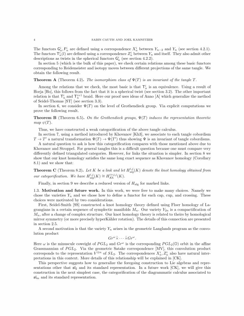
f ca b de
PSfrag replacements
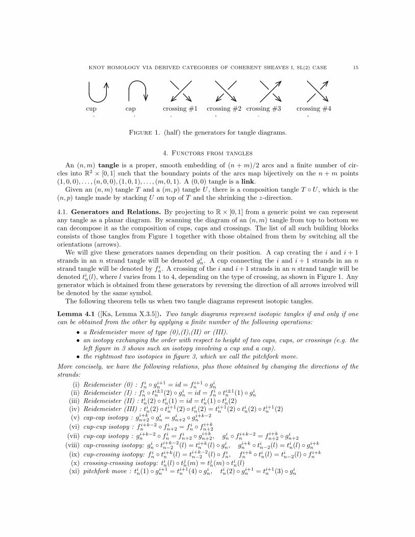
cup cap crossing #1 crossing #2 crossing #3 crossing #4
Figure 1. (half) the generators for tangle diagrams.
4. Functors from tangles
An (n,m) tangle is a proper, smooth embedding of (n + m)/2 arcs and a finite number of cir-cles into R2 × [0, 1] such that the boundary points of the arcs map bijectively on the n + m points(1, 0, 0), . . . , (n, 0, 0), (1, 0, 1), . . . , (m, 0, 1). A (0, 0) tangle is a link.
Given an (n,m) tangle T and a (m, p) tangle U , there is a composition tangle T U , which is the(n, p) tangle made by stacking U on top of T and the shrinking the z-direction.
4.1. Generators and Relations. By projecting to R × [0, 1] from a generic point we can representany tangle as a planar diagram. By scanning the diagram of an (n,m) tangle from top to bottom wecan decompose it as the composition of cups, caps and crossings. The list of all such building blocksconsists of those tangles from Figure 1 together with those obtained from them by switching all theorientations (arrows).
We will give these generators names depending on their position. A cap creating the i and i + 1strands in an n strand tangle will be denoted gin. A cup connecting the i and i + 1 strands in an nstrand tangle will be denoted by f in. A crossing of the i and i+1 strands in an n strand tangle will bedenoted tin(l), where l varies from 1 to 4, depending on the type of crossing, as shown in Figure 1. Anygenerator which is obtained from these generators by reversing the direction of all arrows involved willbe denoted by the same symbol.
The following theorem tells us when two tangle diagrams represent isotopic tangles.
Lemma 4.1 ([Ka, Lemma X.3.5]). Two tangle diagrams represent isotopic tangles if and only if onecan be obtained from the other by applying a finite number of the following operations:
• a Reidemeister move of type (0),(I),(II) or (III).• an isotopy exchanging the order with respect to height of two caps, cups, or crossings (e.g. theleft figure in 3 shows such an isotopy involving a cup and a cap).• the rightmost two isotopies in figure 3, which we call the pitchfork move.
More concisely, we have the following relations, plus those obtained by changing the directions of thestrands:
(i) Reidemeister (0) : f in gi+1n = id = f i+1
n gin(ii) Reidemeister (I) : f in t
i±1n (2) gin = id = f in t
i±1n (1) gin
(iii) Reidemeister (II) : tin(2) tin(1) = id = tin(1) t
in(2)
(iv) Reidemeister (III) : tin(2) ti+1n (2) tin(2) = ti+1
n (2) tin(2) ti+1n (2)
(v) cap-cap isotopy : gi+kn+2 gin = gin+2 g
i+k−2n
(vi) cup-cup isotopy : f i+k−2n f in+2 = f in f
i+kn+2
(vii) cup-cap isotopy : gi+k−2n f in = f in+2 g
i+kn+2, gin f
i+k−2n = f i+kn+2 g
in+2
(viii) cap-crossing isotopy: gin ti+k−2n−2 (l) = ti+kn (l) gin, gi+kn tin−2(l) = tin(l) g
i+kn
(ix) cup-crossing isotopy: f in ti+kn (l) = ti+k−2
n−2 (l) f in, f i+kn tin(l) = tin−2(l) fi+kn
(x) crossing-crossing isotopy: tin(l) tjn(m) = tjn(m) tin(l)
(xi) pitchfork move : tin(1) gi+1n = ti+1
n (4) gin, tin(2) gi+1n = ti+1
n (3) gin
16 SABIN CAUTIS AND JOEL KAMNITZER
PSfrag replacements
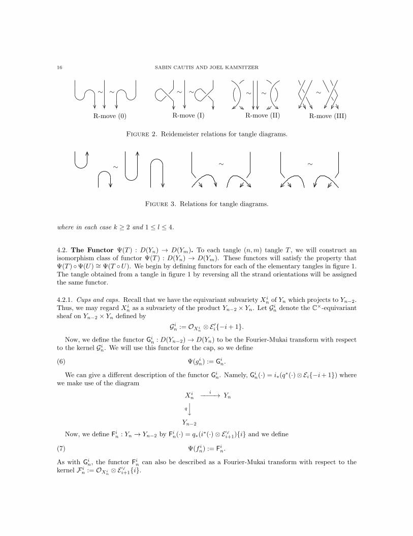
R-move (0) R-move (I) R-move (II) R-move (III)
∼ ∼∼ ∼∼∼∼
Figure 2. Reidemeister relations for tangle diagrams.
PSfrag replacements
∼∼ ∼
Figure 3. Relations for tangle diagrams.
where in each case k ≥ 2 and 1 ≤ l ≤ 4.
4.2. The Functor Ψ(T ) : D(Yn) → D(Ym). To each tangle (n,m) tangle T , we will construct anisomorphism class of functor Ψ(T ) : D(Yn) → D(Ym). These functors will satisfy the property thatΨ(T ) Ψ(U) ∼= Ψ(T U). We begin by defining functors for each of the elementary tangles in figure 1.The tangle obtained from a tangle in figure 1 by reversing all the strand orientations will be assignedthe same functor.
4.2.1. Cups and caps. Recall that we have the equivariant subvariety X in of Yn which projects to Yn−2.
Thus, we may regard X in as a subvariety of the product Yn−2 × Yn. Let Gin denote the C×-equivariant
sheaf on Yn−2 × Yn defined by
Gin := OXin⊗ E ′i−i+ 1.
Now, we define the functor Gin : D(Yn−2)→ D(Yn) to be the Fourier-Mukai transform with respectto the kernel Gin. We will use this functor for the cap, so we define
(6) Ψ(gin) := Gin.
We can give a different description of the functor Gin. Namely, Gin(·) = i∗(q∗(·)⊗Ei−i+ 1) where
we make use of the diagram
X in
i−−−−→ Yn
q
y
Yn−2
Now, we define Fin : Yn → Yn−2 by F
in(·) = q∗(i
∗(·)⊗ E∨i+1)i and we define
(7) Ψ(f in) := Fin.
As with Gin, the functor F
in can also be described as a Fourier-Mukai transform with respect to the
kernel F in := OXin⊗ E∨i+1i.
KNOT HOMOLOGY VIA DERIVED CATEGORIES OF COHERENT SHEAVES I, SL(2) CASE 17
4.2.2. Crossings. Consider the C×-equivariant subvariety
Zin := (L·, L′·) : Lj = L′
j for j 6= i ⊂ Yn × Yn.
Zin has two smooth irreducible components, each of dimension n. The first component corresponds tothe locus of points where Li = L′
i, and so is the diagonal ∆ ⊂ Yn × Yn. The second component is theclosure of the locus of points where Li 6= L′
i. Note that if Li 6= L′i, then zLi+1 ⊂ Li ∩ L′
i = Li−1.Thus we see that on this closure, zLi+1 = Li−1. Hence this second component is the subvarietyV in := X i
n ×Yn−2X in where the fibre product is with respect to the map q : X i
n → Yn−2. Thus
Zin = ∆ ∪ V in ⊂ Yn × Yn.To a crossing connecting boundary points i and i + 1 we assign a Fourier-Mukai kernel T in(l) ∈
D(Yn × Yn) according to the type of crossing:
• crossing #1: T in(1) := OZin[1]−1
• crossing #2: T in(2) := OZin⊗ E∨i+1 ⊗ E
′i[−1]3
• crossing #3: T in(3) := OZin[−1]2
• crossing #4: T in(4) := OZin⊗ E∨i+1 ⊗ E
′i[1]
Now that we have these kernels, we associate to each crossing a functor
(8) Ψ(tin(l)) := Tin(l) := ΦT i
n(l)
where as usual l runs from 1 to 4.
4.2.3. Functor for a tangle. Let T be a tangle. Scanning a projection of T from top to bottom andcomposing along the way gives us a functor Ψ(T ) : D(Yn) → D(Ym). However, this functor maydepend on the choice of tangle projection.
Theorem 4.2. The isomorphism class of the functor Ψ(T ) : D(Yn)→ D(Ym) associated to the planardiagram of an (n,m) tangle T is a tangle invariant.
To prove this theorem, we must check that the functors assigned to the elementary tangles satisfythe relations from Lemma 4.1. This will be done in section 5.
This construction associates to any link L a functor Ψ(L) : D(Y0)→ D(Y0). Since Y0 is a point withthe trivial action of C×, ΨL is determined by Ψ(L)(C) ∈ D(Y0) which is a complex of graded vector
spaces. We denote by Hi,jalg(L) the j-graded piece of the ith cohomology group of Ψ(L)(C) (so i marks
the cohomological degree and j marks the graded degree). Since Ψ(L) is a tangle invariant Hi,jalg(L) isan invariant of the link L.
4.3. Properties of the kernels. Before continuing we mention a few technical results which we willneed later.
Lemma 4.3. If i is the equivariant inclusion X in → Yn and q the equivariant projection X i
n → Yn−2
then
(i) OYn(X i
n)∼= E∨i+1 ⊗ Ei2,
(ii) ωXin⊗ i∗ω∨
Yn
∼= OXin(X i
n)∼= i∗(E∨i+1 ⊗ Ei)2
∼= ωXin⊗ q∗ω∨
Yn−22 so that, in particular,
i∗ωYn∼= q∗ωYn−2
2,
(iii) ωV in
∼= OV in⊗ Ei ⊗ E∨i+1 ⊗ E
′i ⊗ E
′∨i+1 ⊗ π
∗1ωYn
2 ∼= OV in⊗ Ei ⊗ E∨i+1 ⊗ E
′i ⊗ E
′∨i+1 ⊗ π
∗2ωYn
2 asC×-equivariant sheaves on Yn × Yn,
(iv) OV in(D) ∼= OV i
n⊗ E∨i ⊗ E
′i+1 where D is the divisor V in ∩∆ inside V in .
Proof. The map z : Li+1 → Li2 induces a morphism Li+1/Li → Li/Li−12 and hence a section ofHomYn
(Ei+1, Ei2). This section is zero precisely over the locus where z maps Li+1 to Li−1, namelyX in. Thus OYn
(X in)∼= E∨i+1⊗Ei2 as long as the section is transverse to the zero section. Since X i
n is
18 SABIN CAUTIS AND JOEL KAMNITZER
smooth it suffices to show that E∨i+1 ⊗Ei is not a multiple of O(X in). This would follow if we can show
they both restrict to the same (non-trivial) line bundle on a subvariety. We take this subvariety to bea P1 fibre of q : X i+1
n → Yn−2. Since X in and X i+1
n intersect transversely in a section of q (see theremark following lemma 5.1) the restriction of X i
n to the fibre is OP1(1). Meanwhile, E∨i+1 restricts tothe dual of the tautological line bundle, namely OP1(1), whereas Ei restricts to the trivial line bundleOP1 so that E∨i+1 ⊗ Ei also restricts to OP1(1). This concludes (i).
For (ii), by the equivariant adjunction formula we get ωXin⊗ i∗ω∨
Yn
∼= OXin(X i
n) which is isomorphic
to i∗(E∨i+1⊗Ei)2 by (i). To show the last equality note that q : X in → Yn−2 is the C×-equivariant P1
bundle P(z−1Li−1/Li−1)→ Yn−2. So the relative dualizing sheaf ωXin⊗ q∗ω∨
Yn−2of q is
Hom(z−1Li−1/Li, Li/Li−1) = i∗(E∨i+1 ⊗ Ei).
For (iii), consider the projection π1 : V in → X in which is the P1 bundle P(z−1Li−1/Li−1) → X i
n.
The relative dualizing sheaf is then Hom(z−1Li−1/L′i, L
′i/Li−1) = E
′∨i+1 ⊗ E
′i. At the same time this
is isomorphic to ωV in⊗ π∗
1ω∨Xi
nwhich from the calculations above is isomorphic to ωV i
n⊗ Ei+1 ⊗ E∨i ⊗
π∗1ω
∨Yn−2. It follows that
ωV in
∼= Ei ⊗ E∨i+1 ⊗ E
′i ⊗ E
∨′
i+1 ⊗ π∗1ωYn
2
while the second isomorphism involving ωV infollows similarly.
On V in consider the equivariant inclusion map Li/Li−1 → Li+1/Li−1 = Li+1/L′i−1 composed with
the equivariant projection Li+1/L′i−1 → Li+1/L
′i. This gives a C
×-equivariant map Li/Li−1 → Li+1/L′i
which vanishes precisely along the locusD where Li = L′i. If this section is transverse to the zero section
this implies OV in(D) ∼= OV i
n⊗E∨i ⊗E
′i+1. Since D is smooth, to check the section is transverse it suffices
to show that E∨i ⊗ E′i+1 is not a multiple of D. This would follow if we can show they both restrict
to the same (non-trivial) line bundle on a subvariety. We take this subvariety to be a P1 fibre ofπ1 : V in → X i
n. Then D restricts to OP1(1) on such a fibre while E∨i and E ′i+1 restrict to OP1(1) andOP1 respectively. This concludes (iv).
The functors Fin and Gin for caps and cups are related by the following Lemma.
Lemma 4.4. We have that F in ∼= GinR[1]−1
∼= GinL[−1]1. In particular,
Fin(·) = q∗(i
∗(·)⊗ E∨i+1)i∼= G
in
R(·)[1]−1 ∼= G
in
L(·)[−1]1.
Proof. The right adjoints of q∗, i∗ and (·) ⊗ Ei are q∗, i! and (·) ⊗ E∨i respectively. Thus G
inR(·) =
q∗(i!(·) ⊗ E∨i )i − 1. Since i : X i
n → Yn is codimension one we find i!(·) = i∗(·) ⊗ ωXin⊗ i∗ω∨
Yn[−1]
so that GinR(·) = q∗(i
∗(·) ⊗ ωXin⊗ i∗ω∨
Yn⊗ E∨i )[−1]i − 1. Finally by lemma 4.3 below we see that
ωXin⊗ i∗ω∨
Yn⊗ E∨i
∼= E∨i+12 so
GinR(·)[1]−1 ∼= q∗(i
∗(·)⊗ E∨i+1)i.
The calculation of the left adjoint GinLfollows similarly from the facts that the left adjoints of q∗
and i∗ are q! and i∗. This time, using that q : X in → Yn−2 a P1 bundle, we have q!(·) = q∗((·) ⊗
ωXin⊗ q∗ω∨
Yn−2)[1] so that Gin
L(·) = q∗(i
∗(·)⊗ωXin⊗ q∗ω∨
Yn−2⊗E∨i )[1]i− 1. By lemma 4.3 we see that
ωXin⊗ q∗ω∨
Yn−2⊗ E∨i
∼= E∨i+1 so
Gin
L(·)[−1]1 ∼= q∗(i
∗(·)⊗ E∨i+1)i.
The statement on the level of kernels follows similarly.
The functors for under and over crossings are related by the following Lemma.
Lemma 4.5. T in(2)L∼= T in(1)

KNOT HOMOLOGY VIA DERIVED CATEGORIES OF COHERENT SHEAVES I, SL(2) CASE 19
Proof. Consider the standard C×-equivariant short exact sequence 0→ O∆(−D)→ OZin→ OV i
n→ 0
where D = V in ∩∆ is a divisor both in V in and ∆. Since D ⊂ ∆ is just X in ⊂ Yn, we see that O∆(D) is
the restriction of the globally defined line bundle E∨i+1 ⊗ E′i2 on Yn × Yn. Dualizing the above short
exact sequence we get the distinguished triangle
O∨V in→ O∨
Zin→ O∨
∆(D)
where the connecting morphism O∨∆(D)[−1]→ O∨
V inis non-zero. Now
O∨∆∼= ω∆ ⊗ ω
∨Yn×Yn
[−codim(∆)] ∼= O∆ ⊗ π∗2ω
∨Yn[−n]
so that O∨∆(D) ∼= O∆ ⊗ E∨i+1 ⊗ E
′i ⊗ π
∗2ω
∨Yn[−n]2. Similarly, using lemma 4.3
O∨V in
∼= ωV in⊗ ω∨
Yn×Yn[−n]
∼= OV in⊗ Ei ⊗ E
∨i+1 ⊗ E
′i ⊗ E
′∨i+1 ⊗ π
∗1ωYn
⊗ ω∨Yn×Yn
[−n]2
∼= OV in⊗ Ei ⊗ E
∨i+1 ⊗ E
′i ⊗ E
′∨i+1 ⊗ π
∗2ω
∨Yn
[−n]2
Tensoring the above distinguished triangle by Ei+1 ⊗ E′∨i ⊗ π
∗2ωYn
[n]−2 and simplifying we get
OV in⊗ Ei ⊗ E
′∨i+1 → O
∨Zi
n⊗ Ei+1 ⊗ E
′∨i ⊗ π
∗2ωYn
[n]−2 → O∆
Using lemma 4.3 we can simplify further to obtain
OV in(−D)→ O∨
Zin⊗ Ei+1 ⊗ E
′∨i ⊗ π
∗2ωYn
[n]−2 → O∆
where the connecting morphism O∆[−1] → OV in(−D) is non-zero. By corollary 4.8 there exists, up
to a non-zero multiple, a unique such map, namely the one coming from the standard sequence 0 →OV i
n(−D)→ OZi
n→ O∆ → 0. Hence O∨
Zin⊗ Ei+1 ⊗ E
′∨i ⊗ π
∗2ωYn
[n]−2 ∼= OZinwhich means
O∨Zi
n
∼= OZin⊗ E∨i+1 ⊗ E
′i ⊗ π
∗2ω
∨Yn
[−n]2.
Consequently
T in(2)L ∼= (OZin⊗ E∨i+1 ⊗ E
′i[−1]3)
∨ ⊗ π∗2ωYn
[n]
∼= OZin⊗ E∨i+1 ⊗ E
′i ⊗ π
∗2ω
∨Yn[−n]2 ⊗ Ei+1 ⊗ E
′∨i [1]−3 ⊗ π∗
2ωYn[n]
∼= OZin[1]−1 = T in(1)
It turns out that the functors associated to crossings can also be described as spherical twists. Theessential reason for this is that Zin has two components, one of which is the diagonal ∆ and the otheris the fibre product V in = X i
n ×Yn−2X in.
Theorem 4.6. The functor Tin(2) is the twist in the functor G
in shifted by [−1]1. In particular
T in(2)∼= TGi
n[−1]1.
Similarly, the kernel of the functors Tin(1), T
in(3) and T
in(4) are given by
T in(1) ∼= (TGin)L[1]−1 and T
in(3)
∼= (TGin)L[−1]2 and T
in(4)
∼= TGin[1]−2.
Proof. We need to show that
OZin⊗ E∨i+1 ⊗ E
′i2 ∼= Cone(P ∗ PR → O∆) ∈ D(Yn−2 × Yn)
where P = OXin⊗ E ′i−i+ 1. By Lemma 4.4, we have PR ∼= OXi
n⊗ E∨i+1[−1]i+ 1.
20 SABIN CAUTIS AND JOEL KAMNITZER
Now we compute P ∗ PR ∈ D(Yn × Yn−2 × Yn). We have
P ∗ PR = π13∗(π∗12OXi
n⊗ E∨i+1[−1]i+ 1 ⊗ π∗
23OXin⊗ E
′′
i −i+ 1)
By corollary 5.4 we know π−112 (X i
n) and π−123 (X
in) intersect transversely. So by lemma 5.5 we have
π∗12OXi
n⊗ π∗
23OXin
∼= OW where W = π−112 (X i
n) and π−123 (X
in) inside Yn × Yn−2 × Yn. The projection
π13 maps W isomorphically onto V in ⊂ Yn × Yn. Using the projection formula we find
P ∗ PR ∼= OV in⊗ E∨i+1 ⊗ E
′i [−1]2.
Since the map P ∗PR → O∆ is obtained through a series of adjunctions it is not identically zero. Fromthe distinguished triangle
O∆ → Cone(P ∗ PR → O∆)→ P ∗ PR[1]
we find that Cone(P ∗ PR → O∆) is a non-trivial extension of OV in⊗ E∨i+1 ⊗ E
′i2 by O∆ which is
supported in degree zero. On the other hand, V in ∩∆ is the divisor X in → ∆ so we have the standard
exact sequence
0→ O∆(−Xin)→ OZi
n→ OV i
n→ 0.
By lemma 4.3 we know OYn(−X i
n)∼= Ei+1⊗E∨i −2 which means O∆(−X i
n)∼= O∆ ⊗Ei+1⊗E
′∨i −2.
So
0→ O∆ → OZin⊗ E∨i+1 ⊗ E
′i2 → OV i
n⊗ E∨i+1 ⊗ E
′i2 → 0.
Thus OZin⊗ E∨i+1 ⊗ E
′i2 is a non-trivial extension of OV i
n⊗ E∨i+1 ⊗ E
′i2 by O∆. Since the same is
true of Cone(P ∗ PR → O∆) it is enough to show that there exists a unique non-trivial such extensionsince then
Cone(P ∗ PR → O∆) ∼= OZin⊗ E∨i+1 ⊗ E
′i2.
We do this by showing that Ext1(OV in⊗ E∨i+1 ⊗ E
′i2,O∆) is one dimensional, or equivalently that
Ext1(OV in,O∆(−X i
n)) is one dimensional. Since ∆ and V in are smooth with ∆ ∩ V in = X in a smooth
divisor in ∆, we know from corollary 4.8 that Hom1Yn×Yn
(OV in,O∆(−X i
n))∼= HomXi
n(OXi
n,OXi
n) is one
dimensional.To see that T in(1)
∼= (TGin)L[1]−1we use Lemma 4.5 above together with the fact that (TP [−1]1)L =
(TP )L[1]−1 which we apply to P = Gin. The expressions for T in(3) and Tin(4) follow similarly.
Lemma 4.7. Let S, S′ ⊂ T be smooth C×-equivariant subvarieties of a smooth quasi-projective varietyT equipped with a C× action. Suppose the scheme theoretic intersection S ∩ S′ ⊂ T is smooth. If F isa C×-equivariant locally free sheaf on S then
Hl(O∨S′ ⊗ i∗F) =
0 if l < cOS∩S′(j∗F ⊗ detNS∩S′/S) if l = c
where i : S → T , c is the codimension of the embedding j : S ∩ S′ → S and NS∩S′/S is the normalbundle of S ∩ S′ ⊂ S.
Proof. We use the sequence of inclusions S ∩ S′ j−→ S
i−→ T where k = i j. From corollary 11.2 of [H]
we know H−l(i∗i∗F) ∼= ∧lN∨S/T ⊗ F where NS/T is the normal bundle of S in T . Since NS/T as well
as F are locally free on S we find H−l(k∗i∗F) ∼= j∗(∧lN∨S/T ⊗F) = ∧
lN∨S/T |S∩S′ ⊗ j∗F . In particular,
taking F = OS , this means H−l(k∗OS) ∼= ∧lN∨S/T |S∩S′ . Similarly, H−l(k∗OS′) ∼= ∧lN∨
S′/T |S∩S′ .
Note that (the cohomology of) O∨S′⊗ i∗F is supported on S∩S′. So to prove the lemma it is enough
to show that for any sheaf G on S ∩ S′ the sheaf Homl(k∗(G),O∨S′ ⊗ i∗F) is equal to 0 if l < c and
equal to Hom(k∗(G),OS∩S′(j∗F ⊗ detNS∩S′/S)) if l = c. By adjunction, we only need to show that
Hl(k!(O∨S′ ⊗ i∗F)) is zero if l < c and OS∩S′(j∗F ⊗ detNS∩S′/S) if l = c.
KNOT HOMOLOGY VIA DERIVED CATEGORIES OF COHERENT SHEAVES I, SL(2) CASE 21
Now k!(·) = k∗(·)⊗ωS∩S′⊗ω∨T |S∩S′ [−s−c] ∼= k∗(·)⊗detNS∩S′/T [−s−c] where s is the codimension
of S → T . Thus
k!(O∨S′ ⊗ i∗F) ∼= k∗(O∨
S′)⊗ k∗i∗F ⊗ detNS∩S′/T [−s− c].
Now k∗(O∨S′) = k∗(OS′)∨ while Hl(k∗OS′) ∼= ∧−lN∨
S′/T |S∩S′ which are all locally free sheaves. Thus
Hl(k∗O∨S′) ∼= ∧lNS′/T |S∩S′ . In particular, k∗O∨
S′ is supported in degrees 0, . . . , s′ where s′ is the
codimension of S′ → T and H0(k∗O∨S′) ∼= OS∩S′ . On the other hand, k∗i∗F is supported in degrees
−s, . . . , 0 with H−s(k∗i∗(F)) ∼= detN∨S/T |S∩S′ ⊗ j∗F . From this it follows that k∗(O∨
S′ ⊗ i∗F) is
supported in degrees ≥ −s so that
Hl(k∗O∨S′ ⊗ k∗i∗F ⊗ detNS∩S′/T [−s− c]) ∼=
0 if l < cdetN∨
S/T |S∩S′ ⊗ j∗(F)⊗ detNS∩S′/T if l = c.
But from the standard short exact sequence 0 → NS∩S′/S → NS∩S′/T → NS/T |S∩S′ → 0 we see thatdetN∨
S/T |S∩S′ ⊗ detNS∩S′/T∼= detNS∩S′/S . The result follows.
Corollary 4.8. Let S, S′ ⊂ T be smooth C×-equivariant subvarieties of a smooth quasi-projectivevariety T equipped with a C× action. Suppose the scheme theoretic intersection D = S ∩ S′ ⊂ Sis a smooth divisor. Then HomT (OS′ [−1],OS(−D)) ∼= HomD(OD,OD) so, in particular, if T isprojective there exists a non-zero (equivariant) map OS′ [−1] → OS(−D) which is unique up to anon-zero multiple.
Proof. By lemma 4.7 we know
ExtlT (OS′ ,OS(−D)) = Hl(O∨S′ ⊗OS(−D)) ∼=
0 if l < 1OS∩S′(−D +NS∩S′/S) if l = 1.
This means
HomT (OS′ [−1],OS(−D)) = H1(T,O∨S′ ⊗OS(−D)) ∼= H0(T,OS∩S′(−D +NS∩S′/S)).
On the other hand, since D = S ∩ S′ ⊂ S is a divisor, NS∩S′/S∼= OS∩S′(D). Hence
HomT (OS′ [−1],OS(−D)) ∼= H0(T,OS∩S′) ∼= HomD(OD,OD).
5. Invariance of Ψ
In the previous section we defined the functor Ψ(T ) by first choosing a planar diagram representationof T . In this section we prove that Ψ does not depend on this choice. To do this we will show that Ψis invariant under the operations described in lemma 4.1.
5.1. Intersection of subvarieties. We begin with some comments concerning intersection of subva-rieties which we will use for proving many of the invariance results.
Lemma 5.1. For 1 ≤ i < j ≤ n− 1 subvarieties X in → Yn and Xj
n → Yn intersect transversely in asmooth subvariety of codimension two.
Proof. Since X in and Xj
n are smooth submanifolds of Yn, it is enough to work with the topological Yn.By Theorem 2.1, Yn ∼= P1n with X i
n taken to Ain. So it suffices to show that Ain and Ajn intersecttransversely. Recall that
Ain := (l1, . . . , li, a(li), li+2, . . . , ln).
If |i− j| > 1 then Ain and Ajn are clearly transverse.If j = i+ 1 then Ain ∩ A
jn = (l1, . . . , li, a(li), li, li+3, . . . , ln), since a2 = 1. So, either lemma 5.3 or
a direct examination shows that the intersection is transverse.
22 SABIN CAUTIS AND JOEL KAMNITZER
Remark 5.2. The intersection X in ∩ X
i+1n ⊂ Yn consists of points (L1, . . . , Ln) ∈ Yn where Li+1 =
z−1(Li−1) and Li+2 = z−1(Li). This means that setwise, as a subvariety of X in, it is the image of the
section of q : X in → Yn−2 given by
sii+1 : (L1, . . . , Ln−2) 7→ (L1, . . . , Li−1, Li, z−1Li−1, z
−1Li, . . . , z−1Ln−2).
Since by lemma 5.1 the intersection of X in and X i+1
n is transverse we get that, as a subscheme of X in,
the scheme theoretic intersection X in ∩X
i+1n is sii+1. Similarly, the scheme theoretic intersection of X i
n
and X i−1n inside X i
n is also given by a section of q : X in → Yn−2, namely
sii−1 : (L1, . . . , Ln−2) 7→ (L1, . . . , Li−1, z−1Li−2, z
−1Li−1, z−1Li, . . . , z
−1Ln−2).
Note that if |i − j| > 1, the intersection of X in and Xj
n as a subscheme of X in is not a section of
q : X in → Yn−2.
Lemma 5.3. Consider the sequence of smooth varieties and morphisms Yf←− X
g−→ Y ′ and Y ′ f ′
←−
X ′ g′
−→ Y ′′ and suppose the maps (f, g) : X → Y × Y ′ and (f ′, g′) : X ′ → Y ′ × Y ′′ are embeddings and
that g and f ′ are smooth. Let X = π−112 (f, g)(X) and X ′ = π−1
23 (f′, g′)(X ′) where π12 and π23 are
the projection maps from Y × Y ′ × Y ′′ to Y × Y ′ and Y ′ × Y ′′. Then X and X ′ intersect transverselyin Y × Y ′ × Y ′′ if and only if g(X) and f ′(X ′) intersect transversely in Y ′. In particular, if g or f ′ is
surjective then X and X ′ intersect transversely.
Proof. To prove that X and X ′ intersect transversely we need to show that at every point of X ∩ X ′
their tangent spaces intersect transversely. Suppose g(X) and f ′(X ′) intersect transversely. Fix a point
p = (p1, p2, p3) ∈ X ∩ X ′ ⊂ Y × Y ′ × Y ′′. It suffices to show that TpX + TpX ′ = Yp1 ⊕ Y′p2 ⊕ Y
′′p3 .
Fix (a, b, c) ∈ Tp1Y ⊕ Tp2Y′ ⊕ Tp3Y
′′. Since g(X) and f ′(X ′) intersect transversely and g, f ′
are smooth we know g∗(T(p1,p2)X) and f ′∗(T(p2,p3)X
′) intersect transversely and so g∗(T(p1,p2)X) +f ′∗(T(p2,p3)X
′) = Tp2Y′. Then there exists x ∈ T(p1,p2)X, x
′ ∈ T(p2,p3)X′ such that g∗(x) + f ′
∗(x′) = b.
Hence (f∗(x), g∗(x), c− g′∗(x′)) ∈ TpX and (a− f∗(x), f ′
∗(x′), g′∗(x
′)) ∈ TpX ′ and these two vectors add
up to (a, b, c). Hence TpX and TpX ′ intersect transversely. The converse is easier.
Corollary 5.4. The following intersections are all transverse:
(i) π−112 (X
in) ∩ π
−123 (Xj
n+2) in Yn−2 × Yn × Yn+2,
(ii) π−112 (X
in) ∩ π
−123 (Xj
n) in Yn × Yn−2 × Yn, if i 6= j.
(iii) π−112 (X
in+2) ∩ π
−123 (Xj
n+2) in Yn × Yn+2 × Yn, if i 6= j,
(iv) π−112 (X
in ×Yn−2
X in) ∩ π
−123 X
jn in Yn × Yn × Yn−2, if i 6= j.
(v) π−112 (X
in ×Yn−2
X in) ∩ π
−123 X
jn+2 in Yn × Yn × Yn+2, if i 6= j.
(vi) π−112 (X
in ×Yn−2
X in) ∩ π
−123 (X
jn ×Yn−2
Xjn) in Yn × Yn × Yn if i 6= j.
Proof. These all follow from applications from Lemma 5.3.For (i), (ii), (v), we use that X i
n+2 → Yn is surjective and so by the lemma the intersection istransverse.
For (iii), (iv), (vi), by Lemma 5.1, the image of X in in Yn is transverse to the image of Xj
n in Yn fori 6= j. Hence by the lemma, the intersections (iii), (iv), (vii) are transverse.
The main reason for proving that certain intersections are transverse is that transverse intersectionsare useful in computing tensor products of structure sheaves, as shown by the following lemma.
Lemma 5.5. Let S1, . . . , Sm ⊂ T and S′1, . . . , S
′n ⊂ T be irreducible subvarieties such that all inter-
sections Si ∩ Sj ⊂ Si and S′i ∩ S
′j ⊂ S′
i are divisors. If all pairs Si and S′j intersect transversely then
OS ⊗OS′ ∼= OS∩S′ where S = ∪iSi and S′ = ∪iS′i.
KNOT HOMOLOGY VIA DERIVED CATEGORIES OF COHERENT SHEAVES I, SL(2) CASE 23
Proof. We need to show Hl(OS ⊗OS′) = 0 if l < 0. We proceed by induction on the total number ofcomponents. The base case is clear so we just need to prove the inductive step. Suppose we have shownHl(OS⊗OS′) = 0 for l < 0 and S = S1∪· · ·∪Sk−1. The inductive step is to show Hl(OS∪Sk
⊗OS′) = 0if l < 0. Consider the short exact sequence
0→ OSk(IS)→ OS∪Sk
→ OS → 0
where IS is the ideal sheaf of S. Since S ∩ Sk ⊂ Sk is a divisor we get OSk(IS) = OSk
(−D). NowHl(OS ⊗OS′) = 0 if l < 0. So it suffices to show Hl(OSk
(−D)⊗OS′) = 0 if l < 0.Notice OSk
(−D)⊗OS′ = i∗(OSk(−D)⊗i∗OS′) where i is the inclusion Sk → T . Since i∗ is exact it is
enough to show Hl(OSk(−D)⊗i∗OS′) = 0 for l < 0. Since tensoring in Sk by OSk
(−D) is exact we justneed to show Hl(i∗OS′) = 0 for l < 0. This is true since by induction Hl(i∗i∗OS′) = Hl(OSk
⊗OS′) = 0for l < 0.
5.2. Invariance Under Reidemeister Move (0). The first relation we deal with is Reidemeistermove (0) from figure 2 which follows from the following identity.
Proposition 5.6. Fi+1n Gin
∼= id ∼= Fin G
i+1n .
Proof. To prove the first isomorphism recall that the functors Fi+1n ,Gin are the Fourier-Mukai transforms
with respect to the kernels F i+1n = OXi+1
n⊗ E∨i+2i+ 1,Gin = OXi
n⊗ E ′i−i+ 1.
By Corollary 5.4, the intersectionW := π−112 (X
in)∩π
−123 (X i+1
n ) inside Yn−2×Yn×Yn−2 is transverse.Moreover
W = (L·, L′·, L
′′· ) :Lj = L′
j for j ≤ i, Lj = zL′j+2 for j ≥ i,
L′′j = L′
j for j ≤ i+ 1, L′′j = zL′
j+2 for j ≥ i+ 1.
Examining this variety closely, we see that both projections, π1, π3 : W → Yn−2, are isomorphismsand in fact π13 maps W isomorphically to the diagonal in Yn−2 × Yn−2. Moreover, as zL′
i+2 = L′i2
and zL′i+1 = L′
i−12, we see that the operator z induces an isomorphism of line bundles E ′i+2∼= E ′i2
on W .Hence the composition F
i+1n Gin is a Fourier-Mukai transform with respect to the kernel
π13∗(π∗12(OXi
n⊗ E ′i−i+ 1)⊗ π∗
23(OXi+1n⊗ E∨i+2i+ 1))
= π13∗(Oπ−112 (Xi
n)⊗Oπ−1
23 (Xi+1n ) ⊗ E
′i ⊗ E
′i+2
∨2)
∼= π13∗(OW ⊗ E′i ⊗ E
′i+2
∨2)
∼= π13∗(OW ) = O∆
Thus, we conclude that Fi+1n Gin
∼= id.The second isomorphism is actually easier to prove. Fin G
i+1n is the Fourier-Mukai transform with
respect to the kernel
π13∗(π∗12(OXi+1
n⊗ E ′i+1−i)⊗ π
∗23(OXi
n⊗ E ′i+1
∨i)) = π13∗(Oπ−1
12 (Xi+1n ) ⊗Oπ−1
23 (Xin))
∼= Oπ13(π−112 (Xi+1
n )∩π−123 (Xi
n))= O∆
5.3. Invariance Under Reidemeister Move (I). We begin with a lemma on non-transverse inter-sections.
Lemma 5.7. Let X be a smooth projective variety with a C× action and let D be a smooth C×-equivariant divisor in X. Let Y, Z be smooth equivariant subvarieties of D and assume that they meettransversely in D. Then we have the following distinguished triangle in D(X),
OY ∩Z ⊗OX(−D)[1]→ OY ⊗OZ → OY ∩Z

24 SABIN CAUTIS AND JOEL KAMNITZER
Proof. Denote by i the equivariant inclusion Y → X and by i2 and i1 the sequence of equivariantinclusions Y → D → X so that i = i2 i1. To compute i∗i
∗OZ = OY ⊗ OZ we first calculate i∗1OZ .Since Z ⊂ D we find thatH0(i∗1OZ)
∼= OZ andH−1(i∗1OZ)∼= OZ(−D) while the rest of the cohomology
groups vanish (see for instance proposition 11.7 of [H]). This means there is a distinguished triangle
OZ(−D)[1]→ i∗1OZ → OZ .
Since Z and Y intersect transversely inside D we get i2∗i∗2OZ
∼= OY ∩Z . Thus we get a distinguishedtriangle
OY ∩Z ⊗ i∗1OX(−D)[1]→ i2∗i
∗2i
∗1OZ → OY ∩Z .
Applying i1∗ and remembering that i1∗i2∗i∗2i
∗1OZ = i∗i
∗OZ = OY ⊗ OZ we get the distinguishedtriangle
OY ∩Z ⊗OX(−D)[1]→ OY ⊗OZ → OY ∩Z .
To prove invariance under Reidemeister move (I) we need to understand the functor Fin Gin(·). We
will eventually see that Fin Gin(·)∼= (·) ⊗C V where V = C[−1]1 ⊕ C[1]−1, but first we need the
following result.
Proposition 5.8. There is a distinguished triangle
O∆[1]−1 → Fin ∗ G
in → O∆[−1]1
where the first map is the adjoint map O∆ → F in ∗ FinL and the second map is the adjoint map
F in ∗ FinR → O∆ via the isomorphisms Gin
∼= F inR[−1]1∼= F inL[1]−1.
Proof. We have
F in ∗ Gin = π13∗(π
∗12(OXi
n⊗ E ′i−i+ 1)⊗ π∗
23(OXin⊗ E∨i+1i))
= π13∗(Oπ−112 (Xi
n)⊗Oπ−1
23 (Xin)⊗ E ′i ⊗ E
′i+1
∨)1
Now the intersection π−112 (X
in) = X i
n × Yn−2 ∩ π−123 (X i
n) = Yn−2 × X in inside Yn−2 × Yn × Yn−2
is not transverse. In particular, both X in × Yn−2 and Yn−2 × X i
n are contained inside the divisorD := Yn−2 × i(X i
n) × Yn−2. (To avoid confusion, in this section we are writing i(X in) when we view
X in as a subvariety of Yn and X i
n when we view it as a subvariety of Yn−2 × Yn or Yn × Yn−2.)So Lemma 5.7 applies in our situation. Let W = X i
n× Yn−2 ∩ Yn−2×X in. Also, we have by Lemma
4.3 that OYn−2×Yn×Yn−2(−D) ∼= E ′i
∨ ⊗ E ′i+1−2. We conclude that there is a distinguished triangle
OW ⊗ E′i∨⊗ E ′i+1[1]−2 → Oπ−1
12 (Xin)⊗Oπ−1
23 (Xin)→ OW .
Tensoring by E ′i ⊗ E′∨i+11 we get a distinguished triangle
π13∗OW [1]−1 → F in ∗ Gin → π13∗(OW ⊗ E
′i ⊗ E
′i+1
∨)1
Now π13(W ) = ∆ ⊂ Yn−2 × Yn−2 where W → ∆ is the projection q : X in → Yn−2. In particular we
get
π13∗(OW )[1] ∼= O∆[1]
Meanwhile, by corollary 4.3 we know that E ′i ⊗ E′i+1
∨restricted to W = X i
n is precisely the relativedualizing sheaf of q. Consequently,
π13∗(OW ⊗ E′i ⊗ E
′i+1
∨) ∼= O∆[−1].
Thus we conclude that there is a distinguished triangle
O∆[1]−1 → Fin ∗ G
in → O∆[−1]1

KNOT HOMOLOGY VIA DERIVED CATEGORIES OF COHERENT SHEAVES I, SL(2) CASE 25
as desired. To show the maps are as claimed we prove that the Hom spaces O∆[1]−1 → F in ∗ Gin and
F in ∗ Gin → O∆[−1]1 are one dimensional. Since the maps in our distinguished triangle are non-zero
and adjoint maps are non-zero this implies they must agree up to a non-zero multiple.Applying the functor Hom(−,O∆[−1]1) to our distinguished triangle we obtain
Hom(O∆[−1]1,O∆[−1]1)→ Hom(F in ∗ Gin,O∆[−1]1)→ Hom(O∆[1]−1,O∆[−1]1).
But Hom(O∆[−1]1,O∆[−1]1) ∼= C since ∆ = Yn is projective while
Hom(O∆[1]−1,O∆[−1]1) = Ext−2(O∆,O∆2) = 0.
Thus Hom(F in ∗ Gin,O∆[−1]1) is at most one dimensional which means that up to a non-zero mul-
tiple there is at most one non-zero map F in ∗ Gin → O∆[−1]1. Similarly, applying the functor
Hom(O∆[1]−1,−) to our distinguished triangle one finds that up to a non-zero multiple there is atmost one non-zero map O∆[1]−1 → F in ∗ G
in.
Now we will show invariance under Reidemeister move (I).
Theorem 5.9. Fin T
i±1n (2) Gin
∼= id ∼= Fin T
i±1n (1) Gin
Proof. We will just prove the left statement, since the right statement follows from taking left adjoints.To prove the left equality it suffices to prove the stronger statement
F in ∗ Ti±1n (2) ∗ Gin
∼= O∆.
Let R = F in ∗ Ti±1n (2) ∗ Gin.
By theorem 4.6, T i±1n (2) ∼= Cone(Gi±1
n ∗ F i±1n [−1]1
βGi±1n−−−−→ O∆)[−1]1. Hence the left hand side
is
R ∼= Cone(F in ∗ Gi±1n ∗ F i±1
n ∗ Gin[−1]Fi
n∗βFin∗G
i±1n
∗Gin
−−−−−−−−−−−→ F in ∗ Gin)[−1]1.
Now, we know from the proof of 5.6 that F in ∗ Gi±1n∼= O∆
∼= F i±1n ∗ Gin. Hence we see that there is
a distinguished triangle
O∆[−1]1ψ−→ F in ∗ G
in →R[1]−1.
where ψ denotes the result of transferring F in ∗ βGi±1n∗ Gin via the isomorphisms F in ∗ G
i±1n ∗ F i±1
n ∗
Gin[−1]1∼= O∆ ∗ O∆[−1]1 ∼= O∆[−1]1.
Now, by Proposition 5.8, there is a distinguished triangle
O∆[1]−1 → Fin ∗ G
in
φ−→ O∆[−1]1
We claim that φ ψ is a non-zero multiple of the identity. Once we know this we will apply Lemma3.5 to conclude that O∆
∼= R. Also from this lemma, we see that
(9) F in ∗ Gin∼= O∆[1]−1 ⊕ O∆[−1]1.
Now we show that φ ψ is a non-zero multiple of the identity. We have Gi±1n R
∼= F i±1n [−1]1 and
F inR∼= Gin[1]−1. Hence by Lemma 3.3 we deduce the commutativity of the diagram
F in ∗ Gi±1n ∗ F i±1
n ∗ Gin[−1]1Fi
n∗βGi±1n
∗Gin
−−−−−−−−−→ F in ∗ Giny βFi
n[−1]1
y
(F in ∗ Gi+1n ) ∗ (F in ∗ G
i+1n )R[−1]1
βFin∗G
i±1n
[−1]1
−−−−−−−−−−−→ O∆[−1]1
Now, by Proposition 5.8, cφ = βFin[−1]1 (where c ∈ C×) and by definition ψ is the composition
of βGi±1n
with the inverses of the isomorphisms F in ∗ Gi±1n ∗ F i±1
n ∗ Gin[−1]1∼= O∆ ∗ O∆[−1]1 ∼=

26 SABIN CAUTIS AND JOEL KAMNITZER
O∆[−1]1. So up to the identifications that we have made, cφ is the right arrow and ψ is the toparrow, and so cφ ψ is the result of transferring βFi
n∗Gi±1n
[−1]1 to a map O∆[−1]1 → O∆[−1]1.
By the naturality of β the diagram
(F in ∗ Gi±1n ) ∗ (F in ∗ G
i±1n )R
βFin∗G
i±1n
−−−−−−→ O∆y∥∥∥
O∆ ∗ O∆
βO∆−−−−→ O∆
commutes. Now βO∆becomes the identity when we identify O∆ ∗ O∆ with O∆. Thus we conclude
that cφ ψ = id. This proves the left equality.
From (9) we immediately deduce the following corollary of our proof.
Corollary 5.10. FinGin(·)∼= (·)[−1]1⊕(·)[1]−1 so if T is a tangle then Ψ(T∪O)(·) ∼= Ψ(T )(·)⊗CV
where V = C[−1]1 ⊕ C[1]−1.
Remark 5.11. In general, let X be a smooth projective variety and consider the embedding as thezero section X → T ∗Xl where C× acts trivially on the base of π : T ∗Xl → X and by t · v 7→ t−lvon the fibres. Consider the natural Koszul resolution of OX in D(T ∗X):
0← OX ← π∗OX ← π∗TX−l ← π∗ ∧2 TX−2l ← . . . .
If we take its dual and tensor with OX we get
OX → Ω1Xl → Ω2
X2l → . . .
where all the maps are zero. Thus we find that
ExtkD(T∗Xl)(OX ,OX) = ⊕i+j=kHj(X,ΩiX)il = ⊕i+j=kH
i,j(X)il
which is a graded version of Dolbeault cohomology.In our case Y2 is nothing but the Hirzebruch surface P(OP1⊕OP1(−2)) with P1 ∼= X1
2 ⊂ Y2 embeddedas the −2 section. The C× action fixes P1 ⊂ Y2 and acts on the fibres by t · [x, y] = [t−2x, y]. Thus
ExtD(Y2)(OP1 ,OP1) ∼= ExtD(T∗P12)(OP1 ,OP1) ∼= ⊕k ⊕i+j=k Hi,j(P1)[−k]2i
which is isomorphic to C ⊕ C[−2]2. Since the bigraded vector space V appearing in the corollaryis F
12 G
12(C) = ExtD(Y2)(OP1 ,OP1)[1]−1 we can identify V with the [1]−1 shift of the graded
Dolbeault cohomology of P1. In the non-equivariant situation this reduces to the [1] shift of thecohomology of P1.
5.4. Invariance Under Reidemeister Moves (II) and (III).
Proposition 5.12. Tin(2) T
in(1)
∼= id ∼= Tin(1) T
in(2)
Proof. Since F in∼= (Gin)R[1]−1, Proposition (5.8) yields the distinguished triangle
O∆ → GinR ∗ G
in → O∆[−2]2
By Lemma 4.4, GinR∼= GinL[−2]2. Also, since Gin = OXi
n⊗ E ′i−i + 1 we have Hom(Gin,G
in) =
Hom(OXin,OXi
n) where we view X i
n as a subvariety of Yn−2 × Yn. Thus, for any k ∈ Z,
Hom(Gin,Gin[j]k) ∼=
C if j = 0 = k0 if j < 0
KNOT HOMOLOGY VIA DERIVED CATEGORIES OF COHERENT SHEAVES I, SL(2) CASE 27
Since dim(Yn−2)− dim(Yn) = −2 the conditions of Theorem 3.4 are satisfied. So the twist in Gin is anequivalence. By Theorem 4.6, the functor T
in(2) is isomorphic to the twist in Gin shifted by [−1]1.
Hence the functor Tin(2) is also an equivalence.Since Tin(2) is an equivalence its inverse is its left adjoint. By Lemma 4.5 its left adjoint is Tin(1).
So Gin is a spherical functor. Now, we verify the hypothesis which ensures the braid relation for the
twists.
Lemma 5.13.TGi+1
n∗ Gin
∼= TGinR∗ Gi+1
n 1 and TGin∗ Gi+1
n∼= TGi+1
n R∗ Gin1
Proof. We first prove the left equality. By definition and Theorem 4.6 we have that
Gin = OXin⊗ E ′i−i+ 1 and TGi
n= OZi
n⊗ E∨i+1 ⊗ E
′i2 and TGi
nR= TGi
nL= OZi
n
Now by Corollary 5.4, π−112 (X
in) is transverse to each of the two components of π−1
23 (Zi+1n ). Let
W = π−112 (X
in) ∩ π
−123 (Zi+1
n ). Note that W is the locus
W = (L·, L′·, L
′′· ) ∈ Yn−2 × Yn × Yn : Lj = L′
j for j ≤ i− 1, Lj = zL′j+2 for j ≥ i− 1,
L′j = L′′
j for j 6= i+ 1.
In particular, considering the definitions of the line bundles, we see that on W we have isomorphismsof line bundles
(10) Ei2 ∼= E′i+2 and E ′i
∼= E ′′i ,
two facts which we will use later.Note that the fibres of π13 restricted to W are all points and that
π13(W ) = (L·, L′·) ∈ Yn−2 × Yn : Lj = L′
j for all j ≤ i− 1, Lj = zL′j+2 for all j ≥ i.
By Lemma 5.5, we see that
π∗12(OXi
n)⊗ π∗
23(OZi+1n
) = Oπ−112 (Xi
n)⊗Oπ−1
23 (Zi+1n )∼= OW
Hence, we have that
(11)
TGi+1n∗ Gin = π13∗(π
∗12(OXi
n⊗ E ′i−i+ 1)⊗ π∗
23(OZi+1n⊗ E∨i+2 ⊗ E
′i+12))
= π13∗(π∗12(OXi
n)⊗ π∗
23(OZi+1n
)⊗ E ′i ⊗ E′i+2
∨⊗ E ′′i+1)−i+ 3
∼= π13∗(OW ⊗ E′i ⊗ E
′i+2
∨⊗ E ′′i+1)−i+ 3
∼= π13∗(OW ⊗ Ei∨ ⊗ E ′′i ⊗ E
′′i+1)−i+ 1
= Oπ13(W ) ⊗ Ei∨ ⊗ E ′i ⊗ E
′i+1−i+ 1
where in the second last step we use the isomorphisms of line bundles (10).Now, we compute the right hand side TGi
nR∗Gi+1
n 1. Again the intersectionW ′ := π−112 X
i+1n ∩π−1
23 Zin
is transverse. We have
W ′ = (L·, L′·, L
′′· ) ∈ Yn−2 × Yn × Yn : Lj = L′
j for j ≤ i, Lj = zL′j+2 for j ≥ i, L′
j = L′′j for j 6= i.
The fibres of π13 restricted to W ′ are again points and we see that
π13(W′) = π13(W ).
Hence we have
(12)
TGinR∗ Gi+1
n 1 = π13∗(π∗12(OXi+1
n⊗ E ′i+1−i)⊗ π
∗23(OZi
n))1
= π13∗(π∗12(OXi+1
n)⊗ π∗
23(OZin)⊗ E ′i+1)−i+ 1
∼= π13∗(OW ′ ⊗ E ′i+1)−i+ 1
28 SABIN CAUTIS AND JOEL KAMNITZER
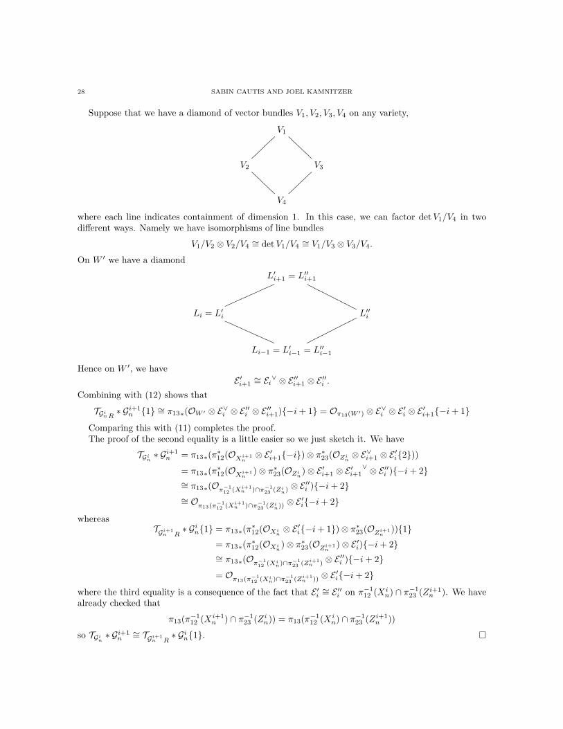
Suppose that we have a diamond of vector bundles V1, V2, V3, V4 on any variety,
V1
V2
V3
AAAAAAA
V4
AAAAAAA
where each line indicates containment of dimension 1. In this case, we can factor detV1/V4 in twodifferent ways. Namely we have isomorphisms of line bundles
V1/V2 ⊗ V2/V4 ∼= det V1/V4 ∼= V1/V3 ⊗ V3/V4.
On W ′ we have a diamond
L′i+1 = L′′
i+1
Li = L′i
mmmmmmmmmmmm
L′′i
OOOOOOOOOOOOO
Li−1 = L′i−1 = L′′
i−1
QQQQQQQQQQQQ
ooooooooooooo
Hence on W ′, we have
E ′i+1∼= Ei
∨ ⊗ E ′′i+1 ⊗ E′′i .
Combining with (12) shows that
TGinR∗ Gi+1
n 1 ∼= π13∗(OW ′ ⊗ E∨i ⊗ E′′i ⊗ E
′′i+1)−i+ 1 = Oπ13(W ′) ⊗ E
∨i ⊗ E
′i ⊗ E
′i+1−i+ 1
Comparing this with (11) completes the proof.The proof of the second equality is a little easier so we just sketch it. We have
TGin∗ Gi+1
n = π13∗(π∗12(OXi+1
n⊗ E ′i+1−i)⊗ π
∗23(OZi
n⊗ E∨i+1 ⊗ E
′i2))
= π13∗(π∗12(OXi+1
n)⊗ π∗
23(OZin)⊗ E ′i+1 ⊗ E
′i+1
∨⊗ E ′′i )−i+ 2
∼= π13∗(Oπ−112 (Xi+1
n )∩π−123 (Zi
n)⊗ E ′′i )−i+ 2
∼= Oπ13(π−112 (Xi+1
n )∩π−123 (Zi
n))⊗ E ′i−i+ 2
whereasTGi+1
n R∗ Gin1 = π13∗(π
∗12(OXi
n⊗ E ′i−i+ 1)⊗ π∗
23(OZi+1n
))1
= π13∗(π∗12(OXi
n)⊗ π∗
23(OZi+1n
)⊗ E ′i)−i+ 2
∼= π13∗(Oπ−112 (Xi
n)∩π−123 (Zi+1
n ) ⊗ E′′i )−i+ 2
= Oπ13(π−112 (Xi
n)∩π−123 (Zi+1
n )) ⊗ E′i−i+ 2
where the third equality is a consequence of the fact that E ′i∼= E ′′i on π−1
12 (Xin) ∩ π
−123 (Z
i+1n ). We have
already checked that
π13(π−112 (X i+1
n ) ∩ π−123 (Z
in)) = π13(π
−112 (X i
n) ∩ π−123 (Z
i+1n ))
so TGin∗ Gi+1
n∼= TGi+1
n R∗ Gin1.
KNOT HOMOLOGY VIA DERIVED CATEGORIES OF COHERENT SHEAVES I, SL(2) CASE 29
Proposition 5.14. The map Ψ is invariant under Reidemeister III moves, ie.
Tin(l) T
i+1n (l′) Tin(l
′′) ∼= Ti+1n (l′′) Tin(l
′) Ti+1n (l)
Proof. We show invariance under the R-move (III) shown in figure 2 (ie l = l′ = l′′ = 2). Reversingthe orientations of some of the strands only changes the twist functors by a shift so it is then easy tocheck that invariance under any R-move of type (III) follows from invariance under the R-move (III)in figure 2.
By Theorem 4.6, we know that Tin(2) is the twist in the spherical functor Gin (shifted by [−1]1).Since for any k ∈ Z and FM kernel P we have TP
∼= TPk, Lemma 5.13 implies
TTGi+1n
∗Gin
∼= TTGinR
∗Gi+1n
and TTGin∗Gi+1
n
∼= TTGi+1n R
∗Gin.
Thus by Theorem 3.7, we see that the twists in the spherical functors Gin and G
i+1n satisfy the braid
relations. Hence Tin(2),T
i+1n (2) satisfy the braid relations.
Remark 5.15. Propositions 5.12, 5.14, and 5.18 show that the functors Tin(2),T
in(1) give a weak
action of the braid group Bn on the derived category of coherent sheaves on Yn. It can be shown thatsimilar functors (given by restricting the kernels from Y2n × Y2n to Un × Un) give a weak action ofB2n on the derived category of coherent sheaves on the open subset Un. Recall that in Proposition2.4 we showed that there was an isomorphism Un with the resolution of a slice to a nilpotent orbit ingl2n. In [B], Bezrukavnikov describes an action of the braid group Bg on the resolution of a slice toany nilpotent orbit in any semisimple Lie algebra g. This action was one of the original motivationsfor our construction and it can be shown that the two constructions coincide.
While our paper was in preparation, the paper [KT] by Khovanov-Thomas appeared. In that paper(among other things), they construct an action of Bn on the derived category of coherent sheaveson the cotangent bundle to the flag variety. The generators of the braid group act as Fourier-Mukaitransforms with respect to kernels similar to our kernels T in(l). They also use the fact that thesefunctors are spherical twists. Their proof of the braid relation is more complicated than ours becausethe geometry of their situation is more complicated.
5.5. Invariance Under Vertical Isotopies From Figure 3.
Proposition 5.16. The functor Ψ is invariant with respect to isotopies exchanging the order withrespect to height of caps and cups. We have
• cap-cap: Gi+kn+2 G
in∼= G
in+2 G
i+k−2n for k ≥ 2.
• cup-cup: Fi+k−2n Fin+2
∼= Fin F
i+kn+2 for k ≥ 2.
• cup-cap: Gi+k−2n Fin
∼= Fin+2 G
i+kn+2 and G
in F
i+k−2n
∼= Fi+kn+2 G
in+2 for k ≥ 2.
Proof. The kernel of Gi+kn+2 Gin : D(Yn−2)→ D(Yn+2) is given by
Gi+kn+2 ∗ Gin = π13∗
(π∗12(G
in)⊗ π
∗23(G
i+kn+2)
)∈ D(Yn−2 × Yn+2).
We have Gin = OXin⊗ E ′i−i + 1 and Gi+kn+2 = OXi+k
n+2
⊗ E ′i+k−i − k + 1. Let W = π−112 (X
in) ∩
π−123 (X i+k
n+2). By Corollary 5.4, this intersection is transverse and so by Lemma 5.5, we have
π∗12(OXi
n)⊗ π∗
23(OXi+kn+2
) ∼= OW .
A routine computation shows that
W = (L·, L′·, L
′′· ) ∈ Yn−2 × Yn × Yn+2 : Lj = L′
j for j ≤ i− 1, Lj = zL′j+2 for j ≥ i− 1,
L′j = L′′
j for j ≤ i+ k − 1, L′j = zL′′
j+2 for j ≥ i+ k − 1.
Hence on W there is an isomorphism of line bundles
(13) E ′i∼= E ′′i
30 SABIN CAUTIS AND JOEL KAMNITZER
The fibres of π13 restricted to W are points and
π13(W ) = (L·, L′·) ∈ Yn−2 × Yn+2 : Lj = L′
j for j ≤ i− 1, Lj = zL′j+2 for i− 1 ≤ j ≤ i+ k − 1,
Lj = z2L′j+4 for j ≥ i+ k − 1.
Hence
(14)
π13∗(π∗12(G
in)⊗ π
∗23(G
i+kn )) = π13∗(Oπ−1
12 (Xin)⊗Oπ−1
23 (Xi+kn+2
) ⊗ E′i ⊗ E
′′i+k)−2i− k + 2
∼= π13∗(OW ⊗ E′i ⊗ E
′′i+k)−2i− k + 2
∼= π13∗(OW ⊗ E′′i ⊗ E
′′i+k)−2i− k + 2
= Oπ13(W ) ⊗ E′i ⊗ E
′i+k−2i− k + 2
where in the second last step we used the above isomorphism (13).Now, we want to compute Gin+2 ∗ G
i+k−2n . Again the intersection W ′ := π−1
12 (X i+k−2n ) ∩ π−1
23 (Xin+2)
is transverse. We have
W ′ = (L·, L′·, L
′′· ) : Lj = L′
j for j ≤ i+ k − 3, Lj = zL′j+2 for j ≥ i+ k − 3,
L′j = L′′
j for j ≤ i− 1, L′j = zL′′
j+2 for j ≥ i+ 1.
Hence on W ′ the map z induces an isomorphism of line bundles
(15) E ′i+k−22 ∼= E′′i+k.
Also we see that the fibres of π13 restricted to W ′ are points and π13(W′) = π13(W ). Hence
(16)
π13∗(π∗12(G
i+k−2n )⊗ π∗
23(Gin+2)) = π13∗(Oπ−1
12 (Xi+k−2n ) ⊗Oπ−1
23 (Xin+2
) ⊗ E′i+k−2 ⊗ E
′′i )−2i− k + 4
∼= π13∗(OW ′ ⊗ E ′i+k−2 ⊗ E′′i )−2i− k + 4
∼= π13∗(OW ′ ⊗ E ′′i+k−2 ⊗ E′′i )−2i− k + 4
= Oπ13(W ) ⊗ E′i ⊗ E
′i+k−2i− k + 2
where in the second last step we have used the isomorphism (15).
Since (14) and (16) agree, we conclude that Gi+kn+2 ∗ Gin∼= Gin+2 ∗ G
i+k−2n and hence that Gi+kn+2 G
in∼=
Gin+2 G
i+k−2n .
The other equations all follow similarly.
Proposition 5.17. The functor Ψ is invariant with respect to isotopies exchanging the order withrespect to height of cap/cups with crossings.
• cap-crossing: Gin T
i+k−2n−2 (l) ∼= T
i+kn (l) Gin for k ≥ 2, 1 ≤ l ≤ 4.
• crossing-cap: Gi+kn Tin−2(l)
∼= Tin(l) G
i+kn for k ≥ 0, 1 ≤ l ≤ 4.
• cup-crossing: Fin T
i+kn (l) ∼= T
i+k−2n−2 (l) Fin for k ≥ 2, 1 ≤ l ≤ 4.
• crossing-cup: Fi+kn Tin(l)
∼= Tin−2(l) F
i+kn for k ≥ 0, 1 ≤ l ≤ 4.
Proof. We will prove the first equation with l = 1.First, note that Gin T
i+k−2n−2 (1) is the Fourier-Mukai transform with respect to the kernel
Gin ∗ Ti+k−2n−2 (1) = π13∗(π
∗12(OZi+k−2
n−2
[1]−1)⊗ π∗23(OXi
n⊗ E ′i−i+ 1))
= π13∗(Oπ−112 (Zi+k−2
n−2) ⊗Oπ−1
23 (Xin))⊗ E ′i [1]−i.
By Corollary 5.4, each component of π−112 (Z
i+k−2n−2 ) intersects π−1
23 (Xin) transversely. Hence by Lemma
5.5, we have that
Oπ−112 (Zi+k−2
n−2) ⊗Oπ−1
23 (Xin)∼= OW
KNOT HOMOLOGY VIA DERIVED CATEGORIES OF COHERENT SHEAVES I, SL(2) CASE 31
where W = π−112 (Z
i+k−2n−2 ) ∩ π−1
23 (X in). We have that
W = (L·, L′·, L
′′· ) : Lj = L′
j for j 6= i+ k − 2, L′j = L′′
j for j ≤ i, L′j = zL′′
j+2 for j ≥ i.
The fibres of π13 restricted to W are just points and so we conclude that
Gin ∗ Ti+k−2n−2 (1) ∼= Oπ13(W ) ⊗ E
′i[1]−i.
On the other hand, using transversality again, we see that
T i+kn (1) ∗ Gin∼= Oπ13(W ′) ⊗ E
′i [1]−i,
where W ′ = π−112 (X i
n) ∩ π−123 (Z
i+kn ). We see that
W ′ = (L·, L′·, L
′′· ) : Lj = L′
j for j ≤ i, Lj = zL′j+2 for j ≥ i, L′
j = L′′j for j 6= i+ k.
A quick inspection of the definitions, shows that
π13(W ) = π13(W′) = (L·, L
′·) : Lj = L′
j for j ≤ i, Lj = zL′j+2 for j ≥ i, j 6= i+ k − 2
whence we conclude that Gin ∗ Ti+k−2n−2 (1) ∼= T i+kn (1) ∗ Gin. The other equations follow similarly.
Proposition 5.18. The functor Ψ is invariant with respect to isotopies exchanging the heights ofcrossings. We have
Tin(l) T
jn(m) ∼= T
jn(m) Tin(l) for 1 ≤ l,m ≤ 4 and |i− j| ≥ 2.
Proof. We will prove the case l = m = 1 (the other cases being similar).As before, we compute the convolution of the Fourier-Mukai kernels. Recall that Zin = ∆ ∪ V in
where V in = X in ×Yn−2
X in. By Corollary 5.4, we see that each component of Zin is transverse to each
component of Zjn. Hence by Lemma 5.5, we have
T in(1) ∗ Tjn (1) = π13∗(π
∗12(OZj
n[1]−1)⊗ π∗
23(OZin[1]−1))
∼= π13∗(OW )[2]−2 = Oπ13(W )[2]−2
where W = π−112 (Z
jn) ∩ π
−123 (Zin) = (L,L
′, L′′) : Lk = L′k for k 6= j, L′
k = L′′k for k 6= i.
A similar computation shows that
T jn (1) ∗ Tin(1)
∼= Oπ13(W ′)[2]−2
where W ′ = (L·, L′·, L
′′· ) : Lk = L′
k for k 6= i, L′k = L′′
k for k 6= j.Since |i− j| ≥ 2, we see that
π13(W ) = π13(W′) = (L·, L
′·) : Lk = L′
k for k 6= i, j,
and so the result follows.
5.6. Invariance under pitchfork move.
Proposition 5.19. Tin(1) G
i+1n∼= T
i+1n (4) Gin, T
in(2) G
i+1n∼= T
i+1n (3) Gin
Proof. We must show that
T in(1) ∗ Gi+1n∼= T i+1
n (4) ∗ Gin and T in(2) ∗ Gi+1n∼= T i+1
n (3) ∗ Gin
But by Theorem 4.6,
T in(1)∼= (TGi
n)R[1]−1, T
i+1n (4) ∼= TGi+1
n[1]−2, T in(2)
∼= TGin[−1]1, T i+1
n (3) ∼= (TGi+1n
)R[−1]2.
So we need to show that
(TGin)R[1]−1 ∗ G
i+1n∼= TGi+1
n[1]−2 ∗ Gin and TGi
n[−1]1 ∗ Gi+1
n∼= (TGi+1
n)R[−1]2 ∗ G
in
which follows from Lemma 5.13.
32 SABIN CAUTIS AND JOEL KAMNITZER
6. The Induced Action on Grothendieck groups
The goal of this section is to prove that on the level of the Grothendieck groups, the geometricallydefined Ψ(T ) induces the representation theoretic map ψ(T ).
6.1. Representation theoretic map. We begin by examining more closely the Reshetikhin-Turaevinvariant of tangles, as discussed in the introduction.
Let V denote the standard representation of Uq(sl2). It is a free C[q, q−1]-module with basis v0, v1.The action of the generators of Uq(sl2) on this basis are
Ev0 = 0, Fv0 = v1, Kv0 = qv0,
Ev1 = v0, Fv1 = v0, Kv1 = q−1v1.
We will now write down explicitly a version of the map
ψ :
(n,m) tangles
→ HomUq(sl2)(V
⊗n, V ⊗m).
discussed in the introduction. We must define ψ(f in), ψ(gin), ψ(t
in(l)). However, since
ψ(gin) = idV ⊗i−1 ⊗ ψ(g12)⊗ idV ⊗n−2−i+1
and similarly for the caps and crossings, it suffices to define ψ(g12), ψ(f12 ), ψ(t
12(l)). For the caps and
cups, we define
ψ(g12) : C[q, q−1]→ V ⊗ V
1 7→ q−1v1 ⊗ v0 − v0 ⊗ v1
ψ(f12 ) : V ⊗ V → C[q, q−1]
v0 ⊗ v0 7→ 0, v0 ⊗ v1 7→ q, v1 ⊗ v0 7→ −1, v1 ⊗ v1 7→ 0
For the crossings, we begin by defining the braiding
β : V ⊗ V → V ⊗ V
v0 ⊗ v0 7→ q1/2v0 ⊗ v0, v0 ⊗ v1 7→ q−1/2v1 ⊗ v0,
v1 ⊗ v0 7→ q−1/2(v0 ⊗ v1 + (q − q−1)v1 ⊗ v0, v1 ⊗ v1 7→ q1/2v1 ⊗ v1
and then define the crossings in terms of the braiding as
ψ(t12(1)) := −q3/2β−1, ψ(t12(2)) := −q
−3/2β, ψ(t12(3)) := −q−3/2β−1, ψ(t12(4)) := q3/2β
Note in particular we have the “Kauffman” relation
(17) ψ(t12(2)) = −q−1β = −q−1(q−1ψ(g11) ψ(f
11 ) + id)
Remark 6.1. These formulas can be obtained from the Reshtikhin-Turaev invariants [RT], with thefollowing caveats. First, we are identifying V ∨ with V via the Uq(sl2)-equivariant isomorphism v0 7→−v1 and v1 7→ q−1v0 (here v0, v1 denote the dual basis). Second, as our “ribbon” element v, we areusing the negative of the usual element. This has the effect of negating the maps assigned to rightmoving caps and cups, and the maps assigned to all of the crossings.
KNOT HOMOLOGY VIA DERIVED CATEGORIES OF COHERENT SHEAVES I, SL(2) CASE 33
6.2. Equivariant K-theory of Yn. First, note that the Grothendieck group K(D(Yn)) is a moduleover C[q, q−1], where q[F ] = [F−1].
To calculate K(D(Yn)) our main tool will be a result from Chriss-Ginzburg [CG], called the cellularfibration lemma. Using this result we will establish a basis for K(D(Yn)).
Theorem 6.2. K(D(Yn)) is a free C[q, q−1] module with basis
∏
j
[Ej ]δjδ∈0,1n
Proof. We proceed by induction on n. As the base case, Y1 ∼= P1 with the trivial C× action. SoK(D(Y1)) is a free C[q, q−1] module with basis [O], [Ei].
We have a C× equivariant fibration π : Yn → Yn−1. This map admits an equivariant section
s : Yn−1 → Yn
(L1, . . . , Ln−1) 7→ (L1, . . . , Ln−1, z−1Ln−2).
The image of this section is Xn−1n . The restriction of π to the compliment π : Yn r Xn−1
n → Yn−1
is an affine fibration, that is, it is a locally trivial bundle with fibres isomorphic to C and transitionfunctions affine linear.
Hence the fibration π along with the filtration Yn ⊃ Xn−1n ⊃ ∅ is a cellular fibration in the sense of
[CG], section 5.5. By induction K(D(Yn−1)) is a free C[q, q−1] module with basis ∏[Ej ]δjδ∈0,1n−1 .
Thus by Lemma 5.5.1 of [CG], K(D(Yn)) is a free C[q, q−1] module with basis
π∗(∏
j<n
[Ej ]δj )δ∈0,1n−1 ∪ s∗(
∏
j<n
[Ej ]δj )δ∈0,1n−1 .
Note that, π∗Ei = Ei by our usual notation, while s∗Ei = OXn−1n⊗ Ei.
Hence K(D(Yn)) is a free C[q, q−1] module with basis
(18) ∏
j<n
[Ej ]δjδ∈0,1n−1 ∪
∏
j<n
[Ej ]δj [OXn−1
n]δ∈0,1n−1.
Now, we have the short exact sequence
0→ OYn(−Xn−1
n )→ OYn→ OXn−1
n→ 0
and also we know by Lemma 4.3 that OYn(−Xn−1
n ) = E∨n−1 ⊗ En−2. Hence we conclude that
[OXn−1n
] = [O]− q2[E∨n−1][En].
Thus by subtracting the first kind of basis vector from the second, then scaling the second kind ofbasis vector and then splitting into two cases depending on δn−1, we see that
(19) ∏
j<n
[Ej ]δjδ∈0,1n−1 ∪
∏
j<n−1
[Ej ]δj [En]δ∈0,1n−2 ∪
∏
j<n−1
[Ej ]δj [E∨n−1][En]δ∈0,1n−2
is a basis.We now claim it suffices to show that
(20) [E∨n−1] = c[En−1] + [V ]
where c ∈ C[q, q−1] is invertible and where [V ] is pulled back from Yn−2. Indeed if this is the case, thenby induction for any δ ∈ 0, 1n−2,
∏j<n−1[Ej ]
δj [V ] is a linear combination of products of distinct [Ej ]
for j < n− 1. Thus,∏j<n−1[Ej ]
δj [V ][En] is a linear combination of the second kind of basis vector in
34 SABIN CAUTIS AND JOEL KAMNITZER
(19). Hence by adding multiples of the second kind of basis vector to the third kind of basis vector, wesee that we can replace the third kind by
∏
j<n−1
[Ej ]δjc[En−1][En].
Since c is invertible we can clear the c to obtain our desired basis.Thus, it remains to establish (20). Consider the short exact sequence
(21) 0→ En−1 → z−1Ln−2/Ln−2 → z−1Ln−2/Ln−1 → 0
This gives us
(22) En−1 ⊗ z−1Ln−2/Ln−1
∼= det(z−1Ln−2/Ln−2) ∼= det(z−1Ln−2)⊗ (detLn−2)∨.
On the other hand we also have the short exact sequence
0→ ker z → z−1Ln−2 → Ln−22 → 0
where the third map is the action of z. This gives us
det(ker z)⊗ det(Ln−22) ∼= det(z−1Ln−2).
Since ker z is spanned by e1 and f1 we find ker z = O22 and hence det(ker z) ∼= O4. We concludethat
det(z−1Ln−2)⊗ (detLn−2)∨ ∼= O2n.
Substituting this back into (22) we see that
z−1Ln−2/Ln−1−2n ∼= E∨n−1.
On the other hand (21) also gives us that
[En−1] + [z−1Ln−2/Ln−1] = [z−1Ln−2/Ln−2]
and so we see that
[En−1]∨ = q2n(−[En−1] + [z−1Ln−2/Ln−2]).
Since z−1Ln−2/Ln−2 is pulled back from Yn−2 we have shown (20) as desired.
Remark 6.3. In the non-equivariant case, a much easier proof is available. First we see thatK(D(Yn)) ∼=K(Yn), the topological K-homology of Yn. Then we use the (non-equivariant) isomorphism of manifoldsYn ∼= (P1)n (Theorem 2.1), to see that
K(D(Yn)) ∼= K((P1)n) ∼= (K(P1))⊗n.
The basis we have given comes from the natural basis of the right hand side.
6.3. Action of basic functors on the Grothendieck groups. We now examine actions of the capsand cups on our basis for K(Yn).
Proposition 6.4. We have
[Gin](∏
j
[Ej ]δj ) = qi−1+2
P
j≥i δj∏
j<i
[Ej ]δj ([Ei]− q
2[Ei+1])∏
j≥i
[Ej+2]δj ,
[Fin](∏
j
[Ej ]δj ) =
0 if δi = δi+1,
q−i−2P
j≥i+2δj∏j<i[Ej ]
δj∏j≥i+2 E
δjj−2 if δi = 0 and δi+1 = 1,
−q−i−2P
j≥i+2 δj∏j<i[Ej]
δj∏j≥i+2 E
δjj−2 if δi = 1 and δi+1 = 0.
KNOT HOMOLOGY VIA DERIVED CATEGORIES OF COHERENT SHEAVES I, SL(2) CASE 35
Proof. First, we consider [Gin]. By definition Gin(F) = i∗q
∗F ⊗ Ei−i + 1. Note that if j < i, thenEj ∼= E ′j on X
in, while if j ≥ i, then Ej2 ∼= E ′j+2 on X i
n. Hence we see that
(23) Gin(⊗
j
Eδjj ) =
⊗
j<i
Eδjj ⊗
⊗
j≥i
Eδjj+2 ⊗OXi
n⊗ Ei−i+ 1− 2
∑
j≥i
δj.
Hence it will be necessary to examine [OXin] in terms of our basis. From the standard short exact
sequence
0→ OYn(−X i
n)→ OYn→ OXi
n→ 0
we have that
[OXin] = [OYn
]− [OYn(−X i
n)] = [OYn]− [Ei+1 ⊗ E
∨i −2].
Using this relation, we can see that (23) gives us
[Gin(⊗
j
Eδjj )] = qi−1+2
P
j≥i δj∏
j<i
[Ej ]δj∏
j≥i
[Ej+2]δj ([OYn
]− [Ei+1 ⊗ E∨i −2])[Ei]
and so first result follows.For the calculation of [Fin], we recall that Fin(F) = q∗(i
∗F ⊗ E∨i+1)i. Now Ei and E∨i+1 restrict toOP1(−1) on the fibres of q, while Ei ⊗ E
∨i+1 is isomorphic to the relative dualizing bundle by Lemma
4.3. Hence we have
Fin(O) = q∗E
∨i+1i = 0, F
in(Ei) = q∗Ei ⊗ E
∨i+1i = O[−1]i,
Fin(Ei+1) = q∗Oi = Oi, F
in(Ei ⊗ Ei+1) = q∗Eii = 0.
From this knowledge, it is easy to deduce the desired description of [Fin].
6.4. Comparison of Grothendieck group with representation. Define a map of C[q, q−1] mod-ules
α : K(D(Yn))→ V ⊗n
∏
i
[Ei]δi 7→ q−
P
i iδivδ1 ⊗ · · · ⊗ vδn .
Theorem 6.5. For any (n,m) tangle T , the following diagram commutes:
(24)
K(D(Yn))[Ψ(T )]−−−−→ K(D(Ym))
α
yyα
V ⊗n −−−−→ψ(T )
V ⊗m
Proof. It suffices to prove the statement when T is a basic tangle, ie. when T = f in, gin, t
in(l).
However, note that by (17), we have ψ(tin(2)) = −q−1(q−1ψ(gin) ψ(f
in) + id). Also since Ψ(tin(2))
is the twist in Gin shifted by [−1]1 (by Theorem 4.6), we have that
[Ψ(tin(2))] = −q−1(−[Gin (Gin)R] + [id])
= −q−1(−[Gin Fin[−1]1] + id) = −q−1(q−1[Ψ(gin)] [Ψ(f in)] + id).
A similar argument for the other tin(l) shows that it actually suffices to prove the statement when T isgin or f in.
36 SABIN CAUTIS AND JOEL KAMNITZER
When T = gin, using Proposition 6.4, following (24) right and down we find∏
j
[Ej]δj 7→ qi−1+2
P
j≥i δj∏
j<i
[Ej]δj ([Ei]− q
2[Ei+1])∏
j≥i
[Ej+2]δj
7→ qi−1+2P
j≥i δj q−P
j<i jδj−P
j≥i(j+2)δjvδ1 ⊗ · · · ⊗ vδi−1⊗
(q−iv1 ⊗ v0 − q−i−1q2v0 ⊗ v1)⊗ vδi ⊗ · · · ⊗ vδn−2
= q−P
j jδjvδ1 ⊗ · · · ⊗ vδi−1⊗ (q−1v1 ⊗ v0 − v0 ⊗ v1)⊗ vδi ⊗ · · · ⊗ vδn−2
.
On the other hand, following (24) down and right we find∏
j
[Ej ]δj 7→ q−
P
j jδjvδ1 ⊗ · · · ⊗ vδn−2
7→ q−P
j jδjvδ1 ⊗ · · · ⊗ vδi−1⊗ (q−1v1 ⊗ v0 − v0 ⊗ v1)⊗ vδi ⊗ · · · ⊗ vδn−2
.
Hence the diagram (24) commutes when T = gin.Now, we consider the case T = f in. There are four cases depending on the values of δi, δi+1. We will
do the case δi = 1, δi+1 = 0. Using proposition 6.4, following (24) right and down we find∏
j<i
[Ej]δj [Ei]
∏
j≥i+2
[Ej ]δj 7→ −q−i−2
P
j>i+1δj∏
j<i
[Ej ]δj
∏
j≥i+2
[Ej−2]δj
7→ −q−i−2P
j≥i+2 δj q−P
j<i jδj−P
j≥i+2(j−2)δjvδ1 ⊗ . . . vδi−1⊗ vδi+2
⊗ · · · ⊗ vδn
= −q−i−P
j jδj vδ1 ⊗ · · · ⊗ vδi−1⊗ vδi+2
⊗ · · · ⊗ vδn .
On the other hand, following (24) down and right we find∏
j<i
[Ej ]δj [Ei]
∏
j≥i+2
[Ej ]δj 7→ q−
P
j jδj−ivδ1 ⊗ · · · ⊗ vδi−1⊗ v1 ⊗ v0 ⊗ vδi+2
⊗ · · · ⊗ vδn
7→ −q−i−P
j jδjvδ1 ⊗ · · · ⊗ vδi−1⊗ vδi+2
⊗ · · · ⊗ vδn ,
and so the diagram commutes. The case where δi = 0, δi+1 = 1 is similar and the two cases whereδi = δi+1 result in both paths giving 0.
Corollary 6.6. If K is a link, then (−1)# of comp of K∑i,j(−1)
iqjdimHijalg(K) is the Jones polynomial.
Proof. First note that by definition∑
i,j
(−1)iqjdimHijalg(K) = [Ψ(K)(C)].
Also by Theorem 6.5, [Ψ(K)(C)] = ψ(K)(1).
Now let ψ denote the “official” Reshetikhin-Turaev invariant, so that ψ(K)(1) is the Jones poly-
nomial. By Remark 6.1 we see that ψ(K) = (−1)r(K)ψ(K) where r(K) denotes the number of rightmoving caps, right moving cups and crossings in a projection of K. Note that r(K) is a link invariant.
We claim that r(K) is the number of components of K. To see this, fix a projection of K and letK ′ be an unlink projection which is obtained from the projection of K by flipping crossings. Hencer(K) = r(K ′). On the other hand K ′ is the unlink, so it has a projection consisting of disjoint circles.Thus, r(K ′) is the number of components of K ′. But K ′ and K have the same number of components,so r(K) is the number of components of K.
Thus combining everything we have that
ψ′(K)(1) = (−1)# of comp of Kψ(K)(1) = (−1)# of comp of K∑
i,j
(−1)iqjdimHijalg(K).
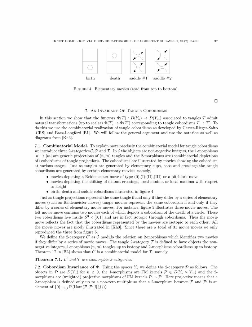
KNOT HOMOLOGY VIA DERIVED CATEGORIES OF COHERENT SHEAVES I, SL(2) CASE 37
PSfrag replacements
birth death saddle #1 saddle #2
Figure 4. Elementary movies (read from top to bottom).
7. An Invariant Of Tangle Cobordisms
In this section we show that the functors Ψ(T ) : D(Yn) → D(Ym) associated to tangles T admitnatural transformations (up to scalar) Ψ(T )→ Ψ(T ′) corresponding to tangle cobordisms T → T ′. Todo this we use the combinatorial realization of tangle cobordisms as developed by Carter-Rieger-Saito[CRS] and Baez-Langford [BL]. We will follow the general argument and use the notation as well asdiagrams from [Kh3].
7.1. Combinatorial Model. To explain more precisely the combinatorial model for tangle cobordismswe introduce three 2-categories C, C′ and T . In C the objects are non-negative integers, the 1-morphisms[n]→ [m] are generic projections of (n,m) tangles and the 2-morphisms are (combinatorial depictionsof) cobordisms of tangle projections. The cobordisms are illustrated by movies showing the cobordismat various stages. Just as tangles are generated by elementary cups, caps and crossings the tanglecobordisms are generated by certain elementary movies: namely,
• movies depicting a Reidemeister move of type (0),(I),(II),(III) or a pitchfork move• movies depicting the shifting of distant crossings, local minima or local maxima with respectto height• birth, death and saddle cobordisms illustrated in figure 4
Just as tangle projections represent the same tangle if and only if they differ by a series of elementarymoves (such as Reidemeister moves) tangle movies represent the same cobordism if and only if theydiffer by a series of elementary movie moves. For instance, figure 5 illustrates three movie moves. Theleft movie move contains two movies each of which depicts a cobordism of the death of a circle. Thesetwo cobordisms live inside S3 × [0, 1] and are in fact isotopic through cobordisms. Thus the moviemove reflects the fact that the cobordisms represented by the movies are isotopic to each other. Allthe movie moves are nicely illustrated in [Kh3]. Since there are a total of 31 movie moves we onlyreproduced the three from figure 5.
We define the 2-category C′ as C modulo the relation on 2-morphisms which identifies two moviesif they differ by a series of movie moves. The tangle 2-category T is defined to have objects the non-negative integers, 1-morphisms (n,m) tangles up to isotopy and 2-morphisms cobordisms up to isotopy.Theorem 17 in [BL] shows that C′ is a combinatorial model for T , namely
Theorem 7.1. C′ and T are isomorphic 2-categories.
7.2. Cobordism Invariance of Ψ. Using the spaces Yn we define the 2-category D as follows. Theobjects in D are D(Yn) for n ≥ 0, the 1-morphisms are FM kernels P ∈ D(Yn × Ym) and the 2-morphisms are (weighted) projective morphisms of FM kernels P → P ′. Here projective means that a2-morphism is defined only up to a non-zero multiple so that a 2-morphism between P and P ′ is anelement of 0 ∪i,j P (Hom(P ,P ′[i]j)).
38 SABIN CAUTIS AND JOEL KAMNITZER
Note that the 1-morphisms P ∈ D(Yn × Ym) induce functors ΦP : D(Yn) → D(Ym). Also, the2-morphisms induce natural transformations of functors ΦP → ΦP′ (up to scalar). Hence there isa natural 2-functor from D to the 2-category of triangulated categories (where we quotient out thenatural transformations by scalars).
We now describe a 2-functor Ψ : C → D. To an object [n] ∈ C we associate D(Yn) ∈ D. To a1-morphism T in C we associate the FM kernel corresponding to the functor Ψ(T ) described in section4.2. To define the 2-functor on 2-morphisms it is enough to associate a (weighted) morphism of FMkernels for each elementary cobordism (if P → P ′[i]j is an equivariant map then the associated mapP → P ′ has weight [i]j):
• to a movie depicting a Reidemeister move of type (0),(I),(II),(III) or a pitchfork move wechoose an isomorphism between the two kernels (we get such isomorphisms from section 5 andany such isomorphism is unique up to scalar multiple)• to a movie depicting the shifting of distant crossings or local minima or maxima we also assignan isomorphism of kernels (we get such isomorphisms from section 5.5 which again are unique)• to the birth cobordism we assign the morphism O∆ → O∆[1]−1 ⊕ O∆[−1]1 of weight[−1]1 given by s 7→ (s, 0)• to the death cobordism we assign the morphism O∆[1]−1 ⊕ O∆[−1]1 → O∆ of weight[−1]1 given by (s, t) 7→ t• to saddle cobordism #1 we assign the natural adjoint map Gin ∗ F
in → O∆ of weight [1]−1
coming from F inL ∗ Fin∼= Gin ∗ G
inR → O∆
• to saddle cobordism #2 we assign the natural adjoint map O∆ → Gin ∗ Fin of weight [1]−1
coming from O∆ → F inR ∗ Fin∼= Gin ∗ G
inL
The fact that Ψ : C → D is a cobordism invariant of tangles is a consequence of the following result.
Theorem 7.2. The morphism of 2-categories Ψ : C → D factors as C → C′ → D.
Proof. We first need the following lemma.
Lemma 7.3. Let Q,Q′ be invertible kernels. If P a kernel corresponding to a planar tangle with noclosed components or crossings then
Hom(Q ∗ P ∗ Q′,Q ∗ P ∗ Q′[i]j) =
0 if i < 0C if i = j = 0
Consequently, Hom(Q∗Gin∗Fin∗Q
′,Q∗O∆∗Q′[1]−1) ∼= C ∼= Hom(Q∗O∆∗Q′,Q∗Gin∗Fin∗Q
′[1]−1).
Proof. SinceQ is invertibleQR∗Q ∼= O∆ and so Hom(Q∗P ,Q∗P) = Hom(P ,QR∗Q∗P) ∼= Hom(P ,P).A similar argument shows that it is enough to consider the case when Q ∼= O∆
∼= Q′.We can write the kernel P corresponding to a planar tangle as the convolution P1∗P2 where P1 is the
convolution of many Gin and P2 the convolution of many F in. Now Fin ∗F
inL = O∆ ⊕O∆[−2]2 = V∆
so P2 ∗ P2L = V ∗m∆ for some non-negative integer m. Consequently
Hom(P ,P) = Hom(P1,P1 ∗ P2 ∗ P2L) = Hom(P1,P1 ∗ V∗m∆ ).
On the other hand, P1 is the convolution of many Gin and hence is isomorphic to a line bundle supportedon a subvariety. This is clear if you recall that the associated functor Gin is i∗(q
∗(·)⊗Ei−i+1) whereq is flat and i is an inclusion. Thus P1
∼= OW (L) where W is some variety and L is some line bundle.Hence P1 ∗ V ∗m
∆ = ⊕i≥0 (OW (L)[−i]i)ni where n0 = 1. The result follows since Hom(OW ,OW ) = C
and Hom(OW ,OW [i]j) = 0 if i < 0.Finally, Hom(Gin ∗ F
in,O∆[1]−1) ∼= Hom(Gin,F
inL[1]−1)
∼= Hom(Gin,Gin)∼= C and similarly
Hom(O∆,Gin ∗ F
in[1]−1)
∼= Hom(GinL,Fin[1]−1)
∼= Hom(F in[1]−1,Fin[1]−1)
∼= C.
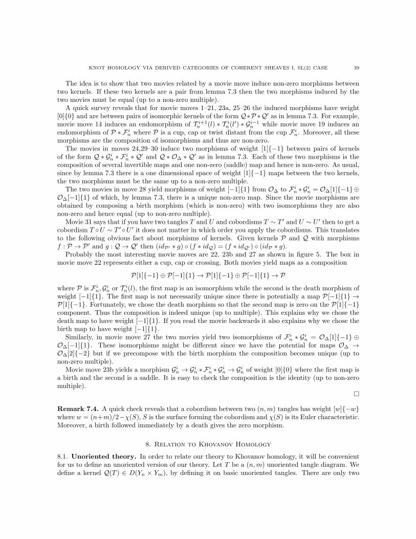
KNOT HOMOLOGY VIA DERIVED CATEGORIES OF COHERENT SHEAVES I, SL(2) CASE 39
The idea is to show that two movies related by a movie move induce non-zero morphisms betweentwo kernels. If these two kernels are a pair from lemma 7.3 then the two morphisms induced by thetwo movies must be equal (up to a non-zero multiple).
A quick survey reveals that for movie moves 1–21, 23a, 25–26 the induced morphisms have weight[0]0 and are between pairs of isomorphic kernels of the form Q∗P ∗Q′ as in lemma 7.3. For example,movie move 14 induces an endomorphism of T i+1
n (l) ∗ T in(l′) ∗ Gi−1
n while movie move 19 induces anendomorphism of P ∗ F in where P is a cup, cap or twist distant from the cup F in. Moreover, all thesemorphisms are the composition of isomorphisms and thus are non-zero.
The movies in moves 24,29–30 induce two morphisms of weight [1]−1 between pairs of kernelsof the form Q ∗ Gin ∗ F
in ∗ Q
′ and Q ∗ O∆ ∗ Q′ as in lemma 7.3. Each of these two morphisms is thecomposition of several invertible maps and one non-zero (saddle) map and hence is non-zero. As usual,since by lemma 7.3 there is a one dimensional space of weight [1]−1 maps between the two kernels,the two morphisms must be the same up to a non-zero multiple.
The two movies in move 28 yield morphisms of weight [−1]1 from O∆ to F in ∗ Gin = O∆[1]−1⊕
O∆[−1]1 of which, by lemma 7.3, there is a unique non-zero map. Since the movie morphisms areobtained by composing a birth morphism (which is non-zero) with two isomorphisms they are alsonon-zero and hence equal (up to non-zero multiple).
Movie 31 says that if you have two tangles T and U and cobordisms T ∼ T ′ and U ∼ U ′ then to get acobordism T U ∼ T ′ U ′ it does not matter in which order you apply the cobordisms. This translatesto the following obvious fact about morphisms of kernels. Given kernels P and Q with morphismsf : P → P ′ and g : Q → Q′ then (idP′ ∗ g) (f ∗ idQ) = (f ∗ idQ′) (idP ∗ g).
Probably the most interesting movie moves are 22, 23b and 27 as shown in figure 5. The box inmovie move 22 represents either a cup, cap or crossing. Both movies yield maps as a composition
P [1]−1 ⊕ P [−1]1 → P [1]−1⊕ P [−1]1 → P
where P is F in,Gin or T in(l), the first map is an isomorphism while the second is the death morphism of
weight [−1]1. The first map is not necessarily unique since there is potentially a map P [−1]1 →P [1]−1. Fortunately, we chose the death morphism so that the second map is zero on the P [1]−1component. Thus the composition is indeed unique (up to multiple). This explains why we chose thedeath map to have weight [−1]1. If you read the movie backwards it also explains why we chose thebirth map to have weight [−1]1.
Similarly, in movie move 27 the two movies yield two isomorphisms of F in ∗ Gin = O∆[1]−1 ⊕
O∆[−1]1. These isomorphisms might be different since we have the potential for maps O∆ →O∆[2]−2 but if we precompose with the birth morphism the composition becomes unique (up tonon-zero multiple).
Movie move 23b yields a morphism Gin → Gin ∗ F
in ∗ G
in → G
in of weight [0]0 where the first map is
a birth and the second is a saddle. It is easy to check the composition is the identity (up to non-zeromultiple).
Remark 7.4. A quick check reveals that a cobordism between two (n,m) tangles has weight [w]−wwhere w = (n+m)/2−χ(S), S is the surface forming the cobordism and χ(S) is its Euler characteristic.Moreover, a birth followed immediately by a death gives the zero morphism.
8. Relation to Khovanov Homology
8.1. Unoriented theory. In order to relate our theory to Khovanov homology, it will be convenientfor us to define an unoriented version of our theory. Let T be a (n,m) unoriented tangle diagram. Wedefine a kernel Q(T ) ∈ D(Yn × Ym), by defining it on basic unoriented tangles. There are only two
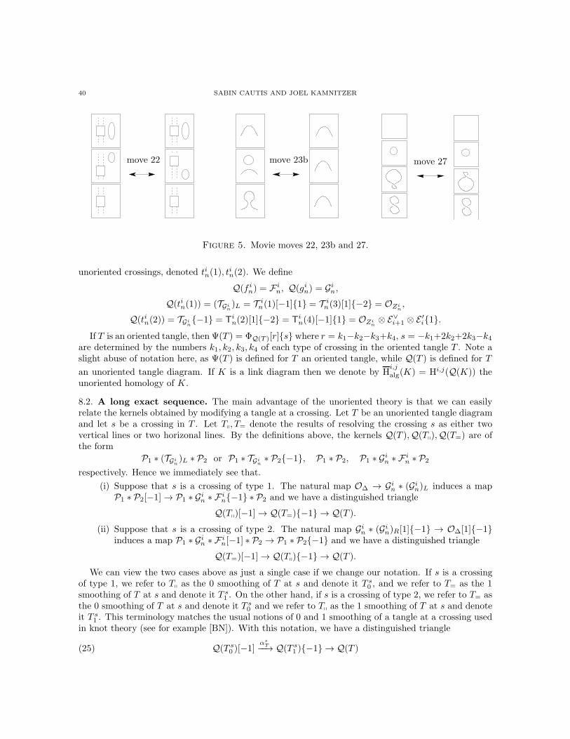
40 SABIN CAUTIS AND JOEL KAMNITZER
PSfrag replacements
move 22 move 23b move 27
Figure 5. Movie moves 22, 23b and 27.
unoriented crossings, denoted tin(1), tin(2). We define
Q(f in) = Fin, Q(g
in) = G
in,
Q(tin(1)) = (TGin)L = T in(1)[−1]1 = T
in(3)[1]−2 = OZi
n,
Q(tin(2)) = TGin−1 = T
in(2)[1]−2 = T
in(4)[−1]1 = OZi
n⊗ E∨i+1 ⊗ E
′i1.
If T is an oriented tangle, then Ψ(T ) = ΦQ(T )[r]s where r = k1−k2−k3+k4, s = −k1+2k2+2k3−k4are determined by the numbers k1, k2, k3, k4 of each type of crossing in the oriented tangle T . Note aslight abuse of notation here, as Ψ(T ) is defined for T an oriented tangle, while Q(T ) is defined for T
an unoriented tangle diagram. If K is a link diagram then we denote by Hi,j
alg(K) = Hi,j(Q(K)) theunoriented homology of K.
8.2. A long exact sequence. The main advantage of the unoriented theory is that we can easilyrelate the kernels obtained by modifying a tangle at a crossing. Let T be an unoriented tangle diagramand let s be a crossing in T . Let Tq, T= denote the results of resolving the crossing s as either twovertical lines or two horizonal lines. By the definitions above, the kernels Q(T ),Q(Tq),Q(T=) are ofthe form
P1 ∗ (TGin)L ∗ P2 or P1 ∗ TGi
n∗ P2−1, P1 ∗ P2, P1 ∗ G
in ∗ F
in ∗ P2
respectively. Hence we immediately see that.
(i) Suppose that s is a crossing of type 1. The natural map O∆ → Gin ∗ (Gin)L induces a map
P1 ∗ P2[−1]→ P1 ∗ Gin ∗ F
in−1 ∗ P2 and we have a distinguished triangle
Q(Tq)[−1]→ Q(T=)−1 → Q(T ).
(ii) Suppose that s is a crossing of type 2. The natural map Gin ∗ (Gin)R[1]−1 → O∆[1]−1
induces a map P1 ∗ Gin ∗ Fin[−1] ∗ P2 → P1 ∗ P2−1 and we have a distinguished triangle
Q(T=)[−1]→ Q(Tq)−1 → Q(T ).
We can view the two cases above as just a single case if we change our notation. If s is a crossingof type 1, we refer to Tq as the 0 smoothing of T at s and denote it T s0 , and we refer to T= as the 1smoothing of T at s and denote it T s1 . On the other hand, if s is a crossing of type 2, we refer to T= asthe 0 smoothing of T at s and denote it T s0 and we refer to Tq as the 1 smoothing of T at s and denoteit T s1 . This terminology matches the usual notions of 0 and 1 smoothing of a tangle at a crossing usedin knot theory (see for example [BN]). With this notation, we have a distinguished triangle
(25) Q(T s0 )[−1]αs
T−−→ Q(T s1 )−1 → Q(T )
KNOT HOMOLOGY VIA DERIVED CATEGORIES OF COHERENT SHEAVES I, SL(2) CASE 41
for any tangle T and any crossing s.We can use this observation to get a long exact sequence for the cohomology of link diagrams.
Corollary 8.1. Let K be a link diagram and let s be a crossing in K. There is a long exact sequence
· · · → Hi−1,j
alg (Ks0)→ H
i,j−1
alg (Ks1)→ H
i,j
alg(K)→ Hi,j
alg(Ks0)→ . . .
Recall that there is another knot homology theory called Khovanov homology which can be definedcompletely combinatorially (see [Kh1]). Let Hi,jKh(K) denote Khovanov homology of a linkK. Khovanovhomology can be defined by first starting with an unoriented theory (which is denoted [[ ]] in [BN])and then correcting it by degree and grading shifts. Unoriented Khovanov homology obeys the samelong exact sequence as in Corollary 8.1. The Khovanov homology of a loop is C−1⊕C1, whereasour homology of a loop is C[1]−1 ⊕ C[−1]1.
From this it is reasonable to expect a relation between Khovanov homology and our cohomologytheory. The remainder of this section is devoted to the proof of the following result.
Theorem 8.2. For any link K,Hi,jalg(K) = Hi+j,jKh (K)
8.3. Convolutions of Complexes. To prove the equivalence with Khovanov homology we will needa notion of cones for complexes of objects in triangulated categories. Thus, we recall the notion ofconvolution introduced by Orlov [O].
Let D be a triangulated category. Let (A•, f•) = A0f1−→ A1 → · · ·
fn−→ An be a sequence of objects
and morphisms in D such that fi+1 fi = 0. Such a sequence is called a complex.A (right) convolution of a complex (A•, f•) is any object B such that there exist
(i) objects A0 = B0, B1, . . . , Bn−1, Bn = B and(ii) morphisms gi : Bi−1 → Ai, hi : Ai → Bi (with h0 = id)
such that
(26) Bi−1gi−→ Ai
hi−→ Bi
is a distinguished triangle for each i and gi hi−1 = fi. Such a collection of data is called a Postnikovsystem. Notice that in a Postnikov system we also have fi+1 gi = (gi+1 hi)gi = 0 since hi gi = 0.
The following result is a sharper version of Lemma 1.5 from [O].
Proposition 8.3. Let (A•, f•) be a complex. The following existence and uniqueness results hold.
(i) If Hom(Ai[k], Ai+k+1) = 0 for all i ≥ 0, k ≥ 1, then any two convolutions of (A•, f•) areisomorphic.
(ii) If Hom(Ai[k], Ai+k+2) = 0 for all i ≥ 0, k ≥ 1, then (A•, f•) has a convolution.
Proof. We start with (i). Let B,B′ be convolutions and let Bi, gi, hi, B′i, g
′i, h
′i be the corresponding
Postnikov systems. We will prove that for all i, Bi ∼= B′i and, using this isomorphism, that gi = g′i, hi =
h′i.First, we show by induction on i that Hom(Bi[k], Ai+k+1) = 0 for all i ≥ 0, k ≥ 1. The base case
of i = 0 is covered by the hypothesis. Now assume i > 0 and consider the long exact sequence comingfrom applying Hom(, Ai+k+1) to the distinguished triangle (26)
Hom(Bi−1[k + 1], Ai+k+1)→ Hom(Bi[k], Ai+k+1)→ Hom(Ai[k], Ai+k+1)
By hypothesis Hom(Ai[k], Ai+k+1) = 0 and by induction Hom(Bi−1[k + 1], Ai+k+1) = 0. ThusHom(Bi[k], Ai+k+1) = 0. Hence for all i ≥ 0, k ≥ 1, Hom(Bi[k], Ai+k+1) = 0. In particularHom(Bi−1[1], Ai+1) = 0.
Now, we are in a position to prove the uniqueness statement. By induction, we assume that i ≥ 1,Bi−1 = B′
i−1 and gi = g′i, hi−1 = h′i−1. Then both Bi, hi and B′i, h
′i give distinguished triangles (26).
42 SABIN CAUTIS AND JOEL KAMNITZER
From the axioms of triangulated categories we see that there is an isomorphism Bi ∼= B′i intertwining
hi and h′i. So it remains to show that this isomorphism intertwines gi+1 and g′i+1. For simplicityassume Bi = B′
i. Now consider the long exact sequence which comes from applying Hom(·, Ai+1) tothe distinguished triangle (26). We see that
Hom(Bi−1[1], Ai+1)→ Hom(Bi, Ai+1)→ Hom(Ai, Ai+1).
Now, gi+1 and g′i+1 lie in the middle group here and both are sent to fi+1 = gi+1 hi = g′i+1 hi underthe right arrow. Since Hom(Bi−1[1], Ai+1) = 0, this forces gi+1 = g′i+1 as desired. By induction wededuce that B ∼= B′ as desired.
For (ii), we must show that there exists a chain B•, g•, h• with the desired properties. Suppose thatwe have constructed B0, . . . , Bi, g1, . . . , gi, h0, . . . , hi. We need to construct gi+1 such that gi+1 hi =
fi+1 and fi+2gi+1 = 0. This is the only obstruction since we then choose Bi+1 = Cone(Bigi+1
−−−→ Ai+1).As above, starting from the hypothesis Hom(Ai[k], Ai+k+2) = 0 for all i ≥ 0, k ≥ 1, we can prove by
induction that Hom(Bi[k], Ai+k+2) = 0 for all i ≥ 0, k ≥ 1 and in particular Hom(Bi−1[1], Ai+2) = 0.Now, we have the two distinguished triangles
Bi−1gi
−−−−→ Aihi−−−−→ Biy
yfi+1
0 −−−−→ Ai+1 −−−−→id
Ai+1
The left square commutes since by induction fi+1 gi = 0. Thus by the axioms of triangulatedcategories, we may choose a morphism gi+1 making this into a commutative diagram of distinguishedtriangles. This will mean that fi+1 = gi+1 hi. However, we might not have fi+2 gi+1 = 0.
To prove this last relation, consider the long exact sequence which comes from applying Hom(·, Ai+2)to the distinguished triangle (26). We see that
Hom(Bi−1[1], Ai+2)→ Hom(Bi, Ai+2)→ Hom(Ai, Ai+2).
Now, fi+2 gi+1 is an element in the middle group and is sent to fi+2 gi+1 hi = fi+2 fi+1 = 0 underthe right arrow. Since, Hom(Bi−1[1], Ai+1) = 0, this forces fi+2 gi+1 = 0 as desired. Thus, we haveproduced gi+1 with the desired properties and hence a convolution exists by this construction.
The behaviour of convolutions under functors is quite easy to understand. Let D1,D2 be triangulatedcategories and let F : D1 → D2 be a triangulated functor. Let (A•, f•) be a complex in D1.
Proposition 8.4. If B is a convolution of (A•, f•) then F(B) is a convolution of (F(A•),F(f•)).
Proof. Since B is a convolution, it comes with a Postnikov system Bi, gi, hi as above. Since F is afunctor and takes distinguished triangles to distinguished triangles, it follows that F(Bi),F(gi),F(hi) isa Postnikov system, and so we see that F(B) is a convolution of (F(A•),F(f•)).
Two examples of unique convolutions worth highlighting. The first example occurs when D is thederived category of an abelian category A. If every term in the complex A0 → A1 → · · · → An is anelement of A ⊂ D then the complex A• in D is the convolution. The second example is when n = 1,in which case the usual cone of A0 → A1 is the unique convolution of this 2-term complex.
The first example can be generalized in the following way (though we may lose uniqueness). Let A
be an abelian category, and let A0f1−→ A1
f2−→ · · ·
fn−→ An be a sequence of objects and morphisms in
Kom(A) (the category of complexes of objects in A) with fi+1 fi = 0. We call such a collection acomplex in Kom(A). SinceKom(A) is not triangulated, this is not covered by our previous definition.
On the other hand, let fi denote the homotopy class of fi. Then (A•, f•) is a complex in K(A) (thehomotopy category of complexes of objects in A).
KNOT HOMOLOGY VIA DERIVED CATEGORIES OF COHERENT SHEAVES I, SL(2) CASE 43
Now, consider the following construction in Kom(A). For each i, we let Bi be the complex with
Bki = Ai+k0 ⊕ · · · ⊕ Aki . Equip Bi with a differential by defining matrix coefficients dkj′j : Ai−j+kj →
Ai−j′+k+1
j′ by
dkj′j =
(−1)i−jdj if j = j′
fj+1 if j′ = j + 1
0 otherwise
where dj denotes the differential in the complex Aj .
We also define maps gi : Bi−1 → Ai by projecting Bi−1 onto Ai−1 and then using fi. The projection
is not a map of complexes, but its composition with fi is (essentially because fi fi−1 = 0). Also the
map hi : Ai → Bi is defined in the obvious way.In this case, we call B = Bn, the convolution of (A•, f•) and we write Con(A•, f•) for B.
Let gi, hi be the homotopy classes of gi, hi. Then (B•, g•, h•) is a Postnikov system and so B is a
convolution of (A•, f•) in K(A). In fact, Con(A•, f•) is nothing more than the total complex of the
double complex Aji with Bi the total complex of the partial double complex A0f0−→ A1
f1−→ · · ·
fi−1
−−−→ Ai.
8.4. Cones from tensor products. Now, we will introduce our main example of complexes andtheir convolutions. Let A be an abelian category with a tensor product ⊗. Recall that K(A) is atriangulated category where ⊗ extends to a bifunctor K(A)×K(A)→ K(A).
Let Cjrj−→ Dj1≤j≤n be a collection of objects and morphisms of K(A). For each j, let Ej be an
object of K(A) such that Ej is a cone of rj .Given this setup, for δ ⊂ 1, . . . , n, we define the object Aδ := Xδ
1 ⊗ · · · ⊗Xδn, where X
δj = Cj if
j /∈ δ and Dj if j ∈ δ. Then, we define Ai := ⊕δ,|δ|=iAδ. In other words Ai is the direct sum of alltensor products with n− i Cjs and i Djs. We define fi : Ai−1 → Ai to be the morphism whose matrixentries fδ′δ : Aδ → Aδ′ are
(27) fδ′δ =
(−1)#k∈δ:k≤j1⊗ rj ⊗ 1 if δ′ = δ ⊔ j
0 otherwise
Here and later, when we write δ′ = δ ⊔ j, we mean that δ′ = δ ∪ j and that j /∈ δ.
Proposition 8.5. (A•, f•) is a complex and E1⊗· · ·⊗En is isomorphic to some convolution of (A•, f•).
Proof. To show that (A•, f•) is complex, we must show that fi+1fi = 0. For this it suffices to considerδ with |δ| = i−1. Let j, k /∈ δ and consider the matrix element of fi+1 fi which is a map Aδ → Aδ⊔j,k.By the definition, this matrix element is the sum
fδ⊔j,k δ⊔j fδ⊔j δ + fδ⊔j,k δ⊔k fδ⊔k δ.
Examining the definition of fδδ′ in (27) we see that these two compositions are the same, except withopposite sign. Thus fi+1 fi = 0 and so (A•, f•) is a complex.
Now it remains to show that E1 ⊗ · · · ⊗ En is isomorphic to a convolution of (A•, f•). To do this,let us first choose a map of complexes rj : Cj → Dj which is a representative for ri. Then we have a
complex Cone(rj) with Cone(rj)k = Ck+1
j ⊕Dkj and with differential given by the matrix
[−dCj
0rj dDj
]
where dCj, dDj
denote the appropriate terms of the differentials for Cj , Dj .
44 SABIN CAUTIS AND JOEL KAMNITZER
By the definition of the triangulated structure in K(A), we have Cone(rj) ∼= Ej . Hence it sufficesto show that Cone(r1)⊗ · · · ⊗ Cone(rn) is a convolution of (A•, f•). Note that by definition
(Cone(r1)⊗ · · · ⊗ Cone(rn)
)k= ⊕δA
k+n−|δ|δ
with differential d having matrix coefficients dkδ′δ : Ak+n−|δ|δ → A
k+1+n−|δ′|δ′ defined by
dkδ′δ =
(−1)n−|δ|dAδif δ′ = δ
(−1)#l∈δ:l≤j1⊗ rj ⊗ 1 = fδ′δ if δ′ = δ ⊔ j
0 otherwise.
The choice of ri as a representative for ri gives us natural choices for representatives fi for the mapsfi. Note that fi+1 fi = 0. Hence we have a complex (A•, f•), in Kom(A). It is easily seen that
Con(A•, f•) = Cone(r1) ⊗ · · · ⊗ Cone(rn) and hence Cone(r1) ⊗ · · · ⊗ Cone(rn) is a convolution of(A•, f•) as desired (see the remarks at the end of section 8.3).
8.5. Cones from tangles. Now we are ready to apply this theory of convolutions to the kernelscoming from tangle diagrams.
Let T be an (n,m) tangle diagram. Recall from above that Q(T ) ∈ D(Yn × Ym) is the kernel thatassociated to T by the unoriented theory. Let S denote the set of crossings in T . Note that S acquiresa total order coming from the order (in terms of height) in which the crossings appear in T . For anysubset δ of S, let Tδ denote the crossingless tangle created by resolving all the crossings of T accordingto the subset δ. That is, a crossing s ∈ S is resolved into the “0-resolution” when s /∈ δ and into the“1-resolution” when s ∈ δ. Let Rδ := Q(Tδ)[|δ| − |S|]−|δ|.
If δ′ = δ ⊔ s, then there is a morphism
(−1)#k∈δ:k≤sαsU [|δ′| − |S|]−|δ| : Rδ → Rδ∪s
where U is the one crossing tangle made by resolving all crossings except s according to δ and leavingthe crossing s (recall that αsU : Q(Tδ)[−1]→ Q(Tδ′)−1).
Now we let Ri = ⊕δ,|δ|=iRδ. We get a complex (R•, h•) by using the above maps as the matrixentries.
Proposition 8.6. Q(T ) is isomorphic to a convolution of (R•, h•).
Proof. By definition, we have Q(T ) = P1 ∗ · · · ∗ Pk where each Pj ∈ D(Ynj−1× Ynj
) is one of
F inj+2,Ginj, (TGi
nj)L, TGi
nj−1 (here n0 = n, nk = m).
It follows from basic properties of the convolution product ∗ that
Q(T ) ∼= π0 k∗(π∗0 1P1 ⊗ · · · ⊗ π
∗k−1 kPk
)
where the tensor products take place in D(Yn0× · · · × Ynk
) and where πi j denotes the projection ontoD(Yni
× Ynj).
Now, define objects and morphisms Cjrj−→ Dj in D(Yn0
× · · · × Ynk) by the following rule
(i) if Pj = F in, then Cj = 0, Dj = π∗j−1 jF
in,
(ii) if Pj = Gin, then Cj = 0, Dj = π∗
j−1 jGin,
(iii) if Pj = (TGin)L, then Cj = π∗
j−1 jO∆[−1], Dj = π∗j−1 jG
in ∗ F
in−1 and rj comes from the
natural map O∆ → Gin ∗ (Gin)L and
(iv) if Pj = TGin−1, then Cj = π∗
j−1 jGin ∗ F
in[−1], Dj = π∗
j−1 jO∆−1 and rj comes from the
natural map Gin ∗ (Gin)R → O∆.
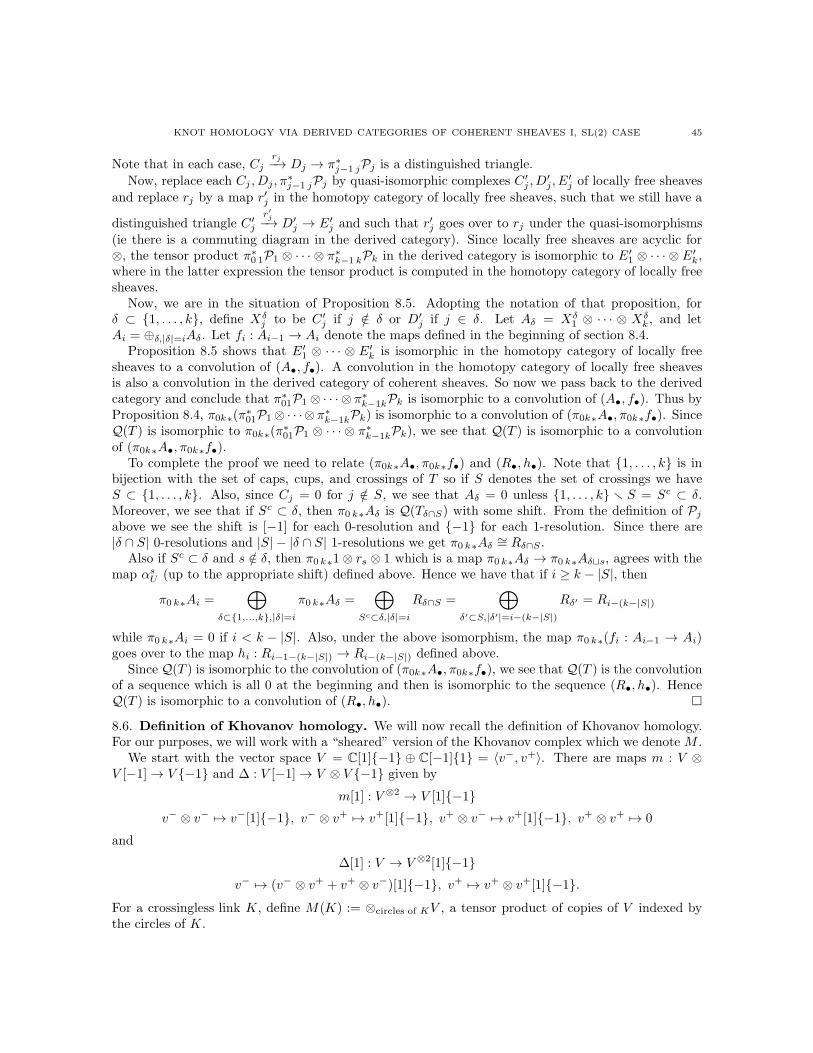
KNOT HOMOLOGY VIA DERIVED CATEGORIES OF COHERENT SHEAVES I, SL(2) CASE 45
Note that in each case, Cjrj−→ Dj → π∗
j−1 jPj is a distinguished triangle.
Now, replace each Cj , Dj, π∗j−1 jPj by quasi-isomorphic complexes C′
j , D′j, E
′j of locally free sheaves
and replace rj by a map r′j in the homotopy category of locally free sheaves, such that we still have a
distinguished triangle C′j
r′j−→ D′
j → E′j and such that r′j goes over to rj under the quasi-isomorphisms
(ie there is a commuting diagram in the derived category). Since locally free sheaves are acyclic for⊗, the tensor product π∗
0 1P1 ⊗ · · · ⊗ π∗k−1 kPk in the derived category is isomorphic to E′
1 ⊗ · · · ⊗ E′k,
where in the latter expression the tensor product is computed in the homotopy category of locally freesheaves.
Now, we are in the situation of Proposition 8.5. Adopting the notation of that proposition, forδ ⊂ 1, . . . , k, define Xδ
j to be C′j if j /∈ δ or D′
j if j ∈ δ. Let Aδ = Xδ1 ⊗ · · · ⊗ Xδ
k , and letAi = ⊕δ,|δ|=iAδ. Let fi : Ai−1 → Ai denote the maps defined in the beginning of section 8.4.
Proposition 8.5 shows that E′1 ⊗ · · · ⊗ E
′k is isomorphic in the homotopy category of locally free
sheaves to a convolution of (A•, f•). A convolution in the homotopy category of locally free sheavesis also a convolution in the derived category of coherent sheaves. So now we pass back to the derivedcategory and conclude that π∗
01P1 ⊗ · · · ⊗ π∗k−1kPk is isomorphic to a convolution of (A•, f•). Thus by
Proposition 8.4, π0k∗(π∗01P1⊗ · · ·⊗ π∗
k−1kPk) is isomorphic to a convolution of (π0k∗A•, π0k∗f•). SinceQ(T ) is isomorphic to π0k∗(π
∗01P1 ⊗ · · · ⊗ π∗
k−1kPk), we see that Q(T ) is isomorphic to a convolutionof (π0k∗A•, π0k∗f•).
To complete the proof we need to relate (π0k∗A•, π0k∗f•) and (R•, h•). Note that 1, . . . , k is inbijection with the set of caps, cups, and crossings of T so if S denotes the set of crossings we haveS ⊂ 1, . . . , k. Also, since Cj = 0 for j /∈ S, we see that Aδ = 0 unless 1, . . . , k r S = Sc ⊂ δ.Moreover, we see that if Sc ⊂ δ, then π0 k∗Aδ is Q(Tδ∩S) with some shift. From the definition of Pjabove we see the shift is [−1] for each 0-resolution and −1 for each 1-resolution. Since there are|δ ∩ S| 0-resolutions and |S| − |δ ∩ S| 1-resolutions we get π0 k∗Aδ ∼= Rδ∩S .
Also if Sc ⊂ δ and s /∈ δ, then π0 k∗1⊗ rs ⊗ 1 which is a map π0 k∗Aδ → π0 k∗Aδ⊔s, agrees with themap αsU (up to the appropriate shift) defined above. Hence we have that if i ≥ k − |S|, then
π0 k∗Ai =⊕
δ⊂1,...,k,|δ|=i
π0 k∗Aδ =⊕
Sc⊂δ,|δ|=i
Rδ∩S =⊕
δ′⊂S,|δ′|=i−(k−|S|)
Rδ′ = Ri−(k−|S|)
while π0 k∗Ai = 0 if i < k − |S|. Also, under the above isomorphism, the map π0 k∗(fi : Ai−1 → Ai)goes over to the map hi : Ri−1−(k−|S|) → Ri−(k−|S|) defined above.
Since Q(T ) is isomorphic to the convolution of (π0k∗A•, π0k∗f•), we see that Q(T ) is the convolutionof a sequence which is all 0 at the beginning and then is isomorphic to the sequence (R•, h•). HenceQ(T ) is isomorphic to a convolution of (R•, h•).
8.6. Definition of Khovanov homology. We will now recall the definition of Khovanov homology.For our purposes, we will work with a “sheared” version of the Khovanov complex which we denote M .
We start with the vector space V = C[1]−1 ⊕ C[−1]1 = 〈v−, v+〉. There are maps m : V ⊗V [−1]→ V −1 and ∆ : V [−1]→ V ⊗ V −1 given by
m[1] : V ⊗2 → V [1]−1
v− ⊗ v− 7→ v−[1]−1, v− ⊗ v+ 7→ v+[1]−1, v+ ⊗ v− 7→ v+[1]−1, v+ ⊗ v+ 7→ 0
and
∆[1] : V → V ⊗2[1]−1
v− 7→ (v− ⊗ v+ + v+ ⊗ v−)[1]−1, v+ 7→ v+ ⊗ v+[1]−1.
For a crossingless link K, define M(K) := ⊗circles of KV , a tensor product of copies of V indexed bythe circles of K.
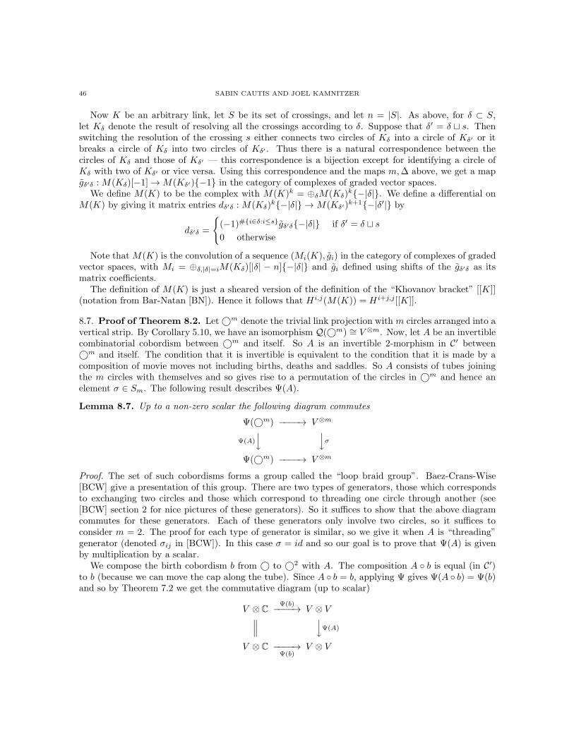
46 SABIN CAUTIS AND JOEL KAMNITZER
Now K be an arbitrary link, let S be its set of crossings, and let n = |S|. As above, for δ ⊂ S,let Kδ denote the result of resolving all the crossings according to δ. Suppose that δ′ = δ ⊔ s. Thenswitching the resolution of the crossing s either connects two circles of Kδ into a circle of Kδ′ or itbreaks a circle of Kδ into two circles of Kδ′ . Thus there is a natural correspondence between thecircles of Kδ and those of Kδ′ — this correspondence is a bijection except for identifying a circle ofKδ with two of Kδ′ or vice versa. Using this correspondence and the maps m,∆ above, we get a mapgδ′δ :M(Kδ)[−1]→M(Kδ′)−1 in the category of complexes of graded vector spaces.
We define M(K) to be the complex with M(K)k = ⊕δM(Kδ)k−|δ|. We define a differential on
M(K) by giving it matrix entries dδ′δ :M(Kδ)k−|δ| →M(Kδ′)
k+1−|δ′| by
dδ′δ =
(−1)#i∈δ:i≤sgδ′δ−|δ| if δ′ = δ ⊔ s
0 otherwise
Note thatM(K) is the convolution of a sequence (Mi(K), gi) in the category of complexes of gradedvector spaces, with Mi = ⊕δ,|δ|=iM(Kδ)[|δ| − n]−|δ| and gi defined using shifts of the gδ′δ as itsmatrix coefficients.
The definition of M(K) is just a sheared version of the definition of the “Khovanov bracket” [[K]](notation from Bar-Natan [BN]). Hence it follows that Hi,j(M(K)) = Hi+j,j [[K]].
8.7. Proof of Theorem 8.2. Let©m denote the trivial link projection with m circles arranged into avertical strip. By Corollary 5.10, we have an isomorphism Q(©m) ∼= V ⊗m. Now, let A be an invertiblecombinatorial cobordism between ©m and itself. So A is an invertible 2-morphism in C′ between©m and itself. The condition that it is invertible is equivalent to the condition that it is made by acomposition of movie moves not including births, deaths and saddles. So A consists of tubes joiningthe m circles with themselves and so gives rise to a permutation of the circles in ©m and hence anelement σ ∈ Sm. The following result describes Ψ(A).
Lemma 8.7. Up to a non-zero scalar the following diagram commutes
Ψ(©m) −−−−→ V ⊗m
Ψ(A)
yyσ
Ψ(©m) −−−−→ V ⊗m
Proof. The set of such cobordisms forms a group called the “loop braid group”. Baez-Crans-Wise[BCW] give a presentation of this group. There are two types of generators, those which correspondsto exchanging two circles and those which correspond to threading one circle through another (see[BCW] section 2 for nice pictures of these generators). So it suffices to show that the above diagramcommutes for these generators. Each of these generators only involve two circles, so it suffices toconsider m = 2. The proof for each type of generator is similar, so we give it when A is “threading”generator (denoted σij in [BCW]). In this case σ = id and so our goal is to prove that Ψ(A) is givenby multiplication by a scalar.
We compose the birth cobordism b from © to ©2 with A. The composition A b is equal (in C′)to b (because we can move the cap along the tube). Since A b = b, applying Ψ gives Ψ(A b) = Ψ(b)and so by Theorem 7.2 we get the commutative diagram (up to scalar)
V ⊗ CΨ(b)−−−−→ V ⊗ V
∥∥∥yΨ(A)
V ⊗ C −−−−→Ψ(b)
V ⊗ V
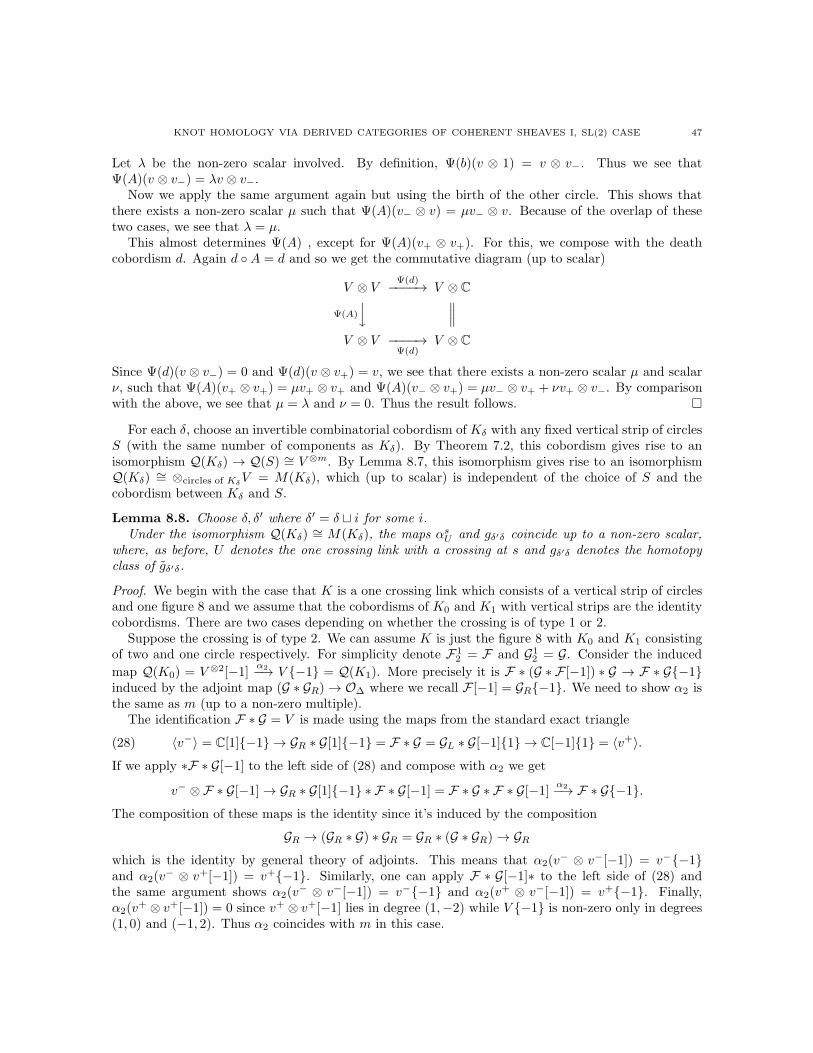
KNOT HOMOLOGY VIA DERIVED CATEGORIES OF COHERENT SHEAVES I, SL(2) CASE 47
Let λ be the non-zero scalar involved. By definition, Ψ(b)(v ⊗ 1) = v ⊗ v−. Thus we see thatΨ(A)(v ⊗ v−) = λv ⊗ v−.
Now we apply the same argument again but using the birth of the other circle. This shows thatthere exists a non-zero scalar µ such that Ψ(A)(v− ⊗ v) = µv− ⊗ v. Because of the overlap of thesetwo cases, we see that λ = µ.
This almost determines Ψ(A) , except for Ψ(A)(v+ ⊗ v+). For this, we compose with the deathcobordism d. Again d A = d and so we get the commutative diagram (up to scalar)
V ⊗ VΨ(d)−−−−→ V ⊗ C
Ψ(A)
y∥∥∥
V ⊗ V −−−−→Ψ(d)
V ⊗ C
Since Ψ(d)(v ⊗ v−) = 0 and Ψ(d)(v ⊗ v+) = v, we see that there exists a non-zero scalar µ and scalarν, such that Ψ(A)(v+ ⊗ v+) = µv+ ⊗ v+ and Ψ(A)(v− ⊗ v+) = µv− ⊗ v+ + νv+ ⊗ v−. By comparisonwith the above, we see that µ = λ and ν = 0. Thus the result follows.
For each δ, choose an invertible combinatorial cobordism of Kδ with any fixed vertical strip of circlesS (with the same number of components as Kδ). By Theorem 7.2, this cobordism gives rise to anisomorphism Q(Kδ) → Q(S) ∼= V ⊗m. By Lemma 8.7, this isomorphism gives rise to an isomorphismQ(Kδ) ∼= ⊗circles of Kδ
V = M(Kδ), which (up to scalar) is independent of the choice of S and thecobordism between Kδ and S.
Lemma 8.8. Choose δ, δ′ where δ′ = δ ⊔ i for some i.Under the isomorphism Q(Kδ) ∼= M(Kδ), the maps αsU and gδ′δ coincide up to a non-zero scalar,
where, as before, U denotes the one crossing link with a crossing at s and gδ′δ denotes the homotopyclass of gδ′δ.
Proof. We begin with the case that K is a one crossing link which consists of a vertical strip of circlesand one figure 8 and we assume that the cobordisms of K0 and K1 with vertical strips are the identitycobordisms. There are two cases depending on whether the crossing is of type 1 or 2.
Suppose the crossing is of type 2. We can assume K is just the figure 8 with K0 and K1 consistingof two and one circle respectively. For simplicity denote F1
2 = F and G12 = G. Consider the induced
map Q(K0) = V ⊗2[−1]α2−→ V −1 = Q(K1). More precisely it is F ∗ (G ∗ F [−1]) ∗ G → F ∗ G−1
induced by the adjoint map (G ∗ GR)→ O∆ where we recall F [−1] = GR−1. We need to show α2 isthe same as m (up to a non-zero multiple).
The identification F ∗ G = V is made using the maps from the standard exact triangle
(28) 〈v−〉 = C[1]−1 → GR ∗ G[1]−1 = F ∗ G = GL ∗ G[−1]1 → C[−1]1 = 〈v+〉.
If we apply ∗F ∗ G[−1] to the left side of (28) and compose with α2 we get
v− ⊗F ∗ G[−1]→ GR ∗ G[1]−1 ∗ F ∗ G[−1] = F ∗ G ∗ F ∗ G[−1]α2−→ F ∗ G−1.
The composition of these maps is the identity since it’s induced by the composition
GR → (GR ∗ G) ∗ GR = GR ∗ (G ∗ GR)→ GR
which is the identity by general theory of adjoints. This means that α2(v− ⊗ v−[−1]) = v−−1
and α2(v− ⊗ v+[−1]) = v+−1. Similarly, one can apply F ∗ G[−1]∗ to the left side of (28) and
the same argument shows α2(v− ⊗ v−[−1]) = v−−1 and α2(v
+ ⊗ v−[−1]) = v+−1. Finally,α2(v
+ ⊗ v+[−1]) = 0 since v+ ⊗ v+[−1] lies in degree (1,−2) while V −1 is non-zero only in degrees(1, 0) and (−1, 2). Thus α2 coincides with m in this case.
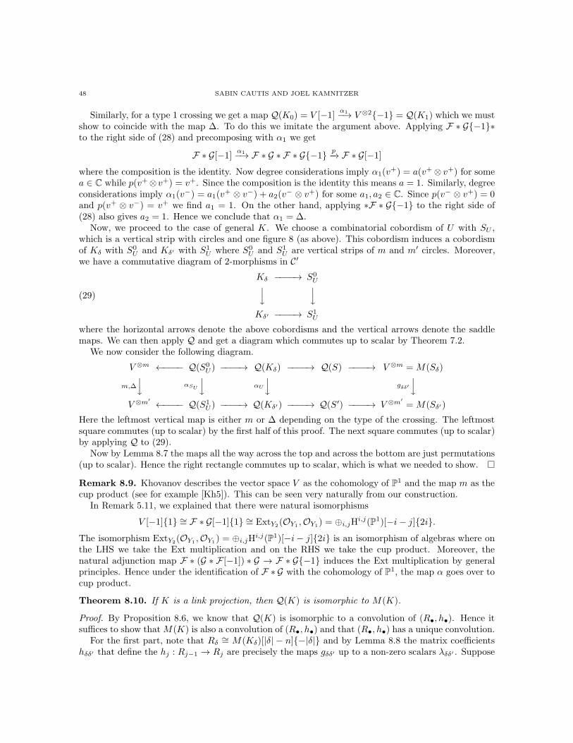
48 SABIN CAUTIS AND JOEL KAMNITZER
Similarly, for a type 1 crossing we get a map Q(K0) = V [−1]α1−→ V ⊗2−1 = Q(K1) which we must
show to coincide with the map ∆. To do this we imitate the argument above. Applying F ∗ G−1∗to the right side of (28) and precomposing with α1 we get
F ∗ G[−1]α1−→ F ∗ G ∗ F ∗ G−1
p−→ F ∗ G[−1]
where the composition is the identity. Now degree considerations imply α1(v+) = a(v+⊗ v+) for some
a ∈ C while p(v+⊗v+) = v+. Since the composition is the identity this means a = 1. Similarly, degreeconsiderations imply α1(v
−) = a1(v+ ⊗ v−) + a2(v
− ⊗ v+) for some a1, a2 ∈ C. Since p(v− ⊗ v+) = 0and p(v+ ⊗ v−) = v+ we find a1 = 1. On the other hand, applying ∗F ∗ G−1 to the right side of(28) also gives a2 = 1. Hence we conclude that α1 = ∆.
Now, we proceed to the case of general K. We choose a combinatorial cobordism of U with SU ,which is a vertical strip with circles and one figure 8 (as above). This cobordism induces a cobordismof Kδ with S0
U and Kδ′ with S1U where S0
U and S1U are vertical strips of m and m′ circles. Moreover,
we have a commutative diagram of 2-morphisms in C′
(29)
Kδ −−−−→ S0Uyy
Kδ′ −−−−→ S1U
where the horizontal arrows denote the above cobordisms and the vertical arrows denote the saddlemaps. We can then apply Q and get a diagram which commutes up to scalar by Theorem 7.2.
We now consider the following diagram.
V ⊗m ←−−−− Q(S0U ) −−−−→ Q(Kδ) −−−−→ Q(S) −−−−→ V ⊗m =M(Sδ)
m,∆
y αSU
y αU
y gδδ′
y
V ⊗m′
←−−−− Q(S1U ) −−−−→ Q(Kδ′) −−−−→ Q(S′) −−−−→ V ⊗m′
=M(Sδ′)
Here the leftmost vertical map is either m or ∆ depending on the type of the crossing. The leftmostsquare commutes (up to scalar) by the first half of this proof. The next square commutes (up to scalar)by applying Q to (29).
Now by Lemma 8.7 the maps all the way across the top and across the bottom are just permutations(up to scalar). Hence the right rectangle commutes up to scalar, which is what we needed to show.
Remark 8.9. Khovanov describes the vector space V as the cohomology of P1 and the map m as thecup product (see for example [Kh5]). This can be seen very naturally from our construction.
In Remark 5.11, we explained that there were natural isomorphisms
V [−1]1 ∼= F ∗ G[−1]1 ∼= ExtY2(OY1
,OY1) = ⊕i,jH
i,j(P1)[−i− j]2i.
The isomorphism ExtY2(OY1
,OY1) = ⊕i,jH
i,j(P1)[−i− j]2i is an isomorphism of algebras where onthe LHS we take the Ext multiplication and on the RHS we take the cup product. Moreover, thenatural adjunction map F ∗ (G ∗ F [−1]) ∗ G → F ∗ G−1 induces the Ext multiplication by generalprinciples. Hence under the identification of F ∗ G with the cohomology of P1, the map α goes over tocup product.
Theorem 8.10. If K is a link projection, then Q(K) is isomorphic to M(K).
Proof. By Proposition 8.6, we know that Q(K) is isomorphic to a convolution of (R•, h•). Hence itsuffices to show thatM(K) is also a convolution of (R•, h•) and that (R•, h•) has a unique convolution.
For the first part, note that Rδ ∼= M(Kδ)[|δ| − n]−|δ| and by Lemma 8.8 the matrix coefficientshδδ′ that define the hj : Rj−1 → Rj are precisely the maps gδδ′ up to a non-zero scalars λδδ′ . Suppose
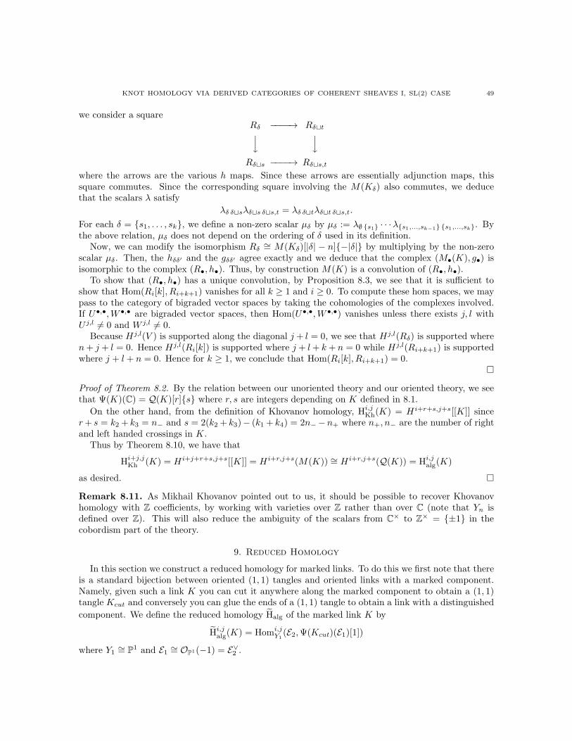
KNOT HOMOLOGY VIA DERIVED CATEGORIES OF COHERENT SHEAVES I, SL(2) CASE 49
we consider a squareRδ −−−−→ Rδ⊔ty
y
Rδ⊔s −−−−→ Rδ⊔s,t
where the arrows are the various h maps. Since these arrows are essentially adjunction maps, thissquare commutes. Since the corresponding square involving the M(Kδ) also commutes, we deducethat the scalars λ satisfy
λδ δ⊔sλδ⊔s δ⊔s,t = λδ δ⊔tλδ⊔t δ⊔s,t.
For each δ = s1, . . . , sk, we define a non-zero scalar µδ by µδ := λ∅ s1 · · ·λs1,...,sk−1 s1,...,sk. Bythe above relation, µδ does not depend on the ordering of δ used in its definition.
Now, we can modify the isomorphism Rδ ∼= M(Kδ)[|δ| − n]−|δ| by multiplying by the non-zeroscalar µδ. Then, the hδδ′ and the gδδ′ agree exactly and we deduce that the complex (M•(K), g•) isisomorphic to the complex (R•, h•). Thus, by construction M(K) is a convolution of (R•, h•).
To show that (R•, h•) has a unique convolution, by Proposition 8.3, we see that it is sufficient toshow that Hom(Ri[k], Ri+k+1) vanishes for all k ≥ 1 and i ≥ 0. To compute these hom spaces, we maypass to the category of bigraded vector spaces by taking the cohomologies of the complexes involved.If U•,•,W •,• are bigraded vector spaces, then Hom(U•,•,W •,•) vanishes unless there exists j, l withU j,l 6= 0 and W j,l 6= 0.
Because Hj,l(V ) is supported along the diagonal j + l = 0, we see that Hj,l(Rδ) is supported wheren+ j + l = 0. Hence Hj,l(Ri[k]) is supported where j + l+ k + n = 0 while Hj,l(Ri+k+1) is supportedwhere j + l + n = 0. Hence for k ≥ 1, we conclude that Hom(Ri[k], Ri+k+1) = 0.
Proof of Theorem 8.2. By the relation between our unoriented theory and our oriented theory, we seethat Ψ(K)(C) = Q(K)[r]s where r, s are integers depending on K defined in 8.1.
On the other hand, from the definition of Khovanov homology, Hi,jKh(K) = Hi+r+s,j+s[[K]] sincer+ s = k2 + k3 = n− and s = 2(k2 + k3)− (k1 + k4) = 2n−−n+ where n+, n− are the number of rightand left handed crossings in K.
Thus by Theorem 8.10, we have that
Hi+j,jKh (K) = Hi+j+r+s,j+s[[K]] = Hi+r,j+s(M(K)) ∼= Hi+r,j+s(Q(K)) = Hi,jalg(K)
as desired.
Remark 8.11. As Mikhail Khovanov pointed out to us, it should be possible to recover Khovanovhomology with Z coefficients, by working with varieties over Z rather than over C (note that Yn isdefined over Z). This will also reduce the ambiguity of the scalars from C× to Z× = ±1 in thecobordism part of the theory.
9. Reduced Homology
In this section we construct a reduced homology for marked links. To do this we first note that thereis a standard bijection between oriented (1, 1) tangles and oriented links with a marked component.Namely, given such a link K you can cut it anywhere along the marked component to obtain a (1, 1)tangle Kcut and conversely you can glue the ends of a (1, 1) tangle to obtain a link with a distinguished
component. We define the reduced homology Halg of the marked link K by
Hi,jalg(K) = Homi,jY1(E2,Ψ(Kcut)(E1)[1])
where Y1 ∼= P1 and E1 ∼= OP1(−1) = E∨2 .
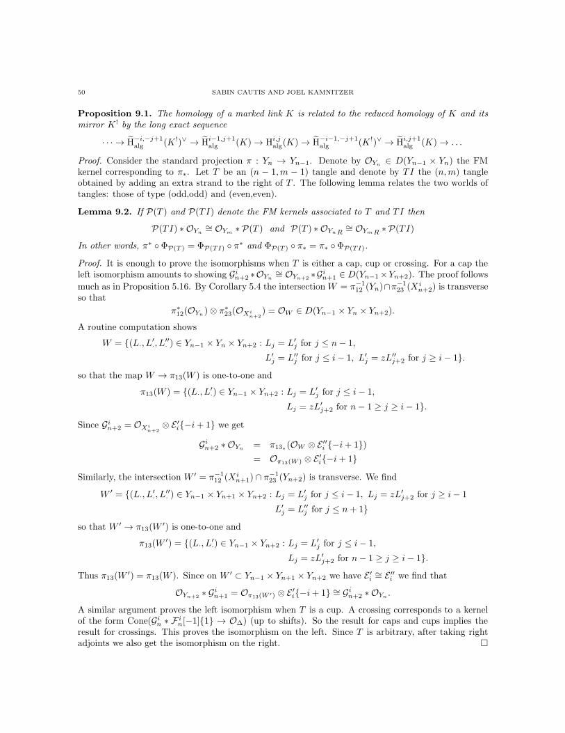
50 SABIN CAUTIS AND JOEL KAMNITZER
Proposition 9.1. The homology of a marked link K is related to the reduced homology of K and itsmirror K ! by the long exact sequence
· · · → H−i,−j+1alg (K !)∨ → Hi−1,j+1
alg (K)→ Hi,jalg(K)→ H−i−1,−j+1alg (K !)∨ → Hi,j+1
alg (K)→ . . .
Proof. Consider the standard projection π : Yn → Yn−1. Denote by OYn∈ D(Yn−1 × Yn) the FM
kernel corresponding to π∗. Let T be an (n − 1,m − 1) tangle and denote by TI the (n,m) tangleobtained by adding an extra strand to the right of T . The following lemma relates the two worlds oftangles: those of type (odd,odd) and (even,even).
Lemma 9.2. If P(T ) and P(TI) denote the FM kernels associated to T and TI then
P(TI) ∗ OYn∼= OYm
∗ P(T ) and P(T ) ∗ OYnR∼= OYmR ∗ P(TI)
In other words, π∗ ΦP(T ) = ΦP(TI) π∗ and ΦP(T ) π∗ = π∗ ΦP(TI).
Proof. It is enough to prove the isomorphisms when T is either a cap, cup or crossing. For a cap theleft isomorphism amounts to showing Gin+2 ∗OYn
∼= OYn+2∗Gin+1 ∈ D(Yn−1×Yn+2). The proof follows
much as in Proposition 5.16. By Corollary 5.4 the intersectionW = π−112 (Yn)∩π
−123 (X i
n+2) is transverseso that
π∗12(OYn
)⊗ π∗23(OXi
n+2) = OW ∈ D(Yn−1 × Yn × Yn+2).
A routine computation shows
W = (L·, L′·, L
′′· ) ∈ Yn−1 × Yn × Yn+2 : Lj = L′
j for j ≤ n− 1,
L′j = L′′
j for j ≤ i− 1, L′j = zL′′
j+2 for j ≥ i− 1.
so that the map W → π13(W ) is one-to-one and
π13(W ) = (L·, L′·) ∈ Yn−1 × Yn+2 : Lj = L′
j for j ≤ i− 1,
Lj = zL′j+2 for n− 1 ≥ j ≥ i− 1.
Since Gin+2 = OXin+2⊗ E ′i−i+ 1 we get
Gin+2 ∗ OYn= π13∗(OW ⊗ E
′′i −i+ 1)
= Oπ13(W ) ⊗ E′i−i+ 1
Similarly, the intersection W ′ = π−112 (X i
n+1) ∩ π−123 (Yn+2) is transverse. We find
W ′ = (L·, L′·, L
′′· ) ∈ Yn−1 × Yn+1 × Yn+2 : Lj = L′
j for j ≤ i− 1, Lj = zL′j+2 for j ≥ i− 1
L′j = L′′
j for j ≤ n+ 1
so that W ′ → π13(W′) is one-to-one and
π13(W′) = (L·, L
′·) ∈ Yn−1 × Yn+2 : Lj = L′
j for j ≤ i− 1,
Lj = zL′j+2 for n− 1 ≥ j ≥ i− 1.
Thus π13(W′) = π13(W ). Since on W ′ ⊂ Yn−1 × Yn+1 × Yn+2 we have E ′i
∼= E ′′i we find that
OYn+2∗ Gin+1 = Oπ13(W ′) ⊗ E
′i−i+ 1 ∼= Gin+2 ∗ OYn
.
A similar argument proves the left isomorphism when T is a cup. A crossing corresponds to a kernelof the form Cone(Gin ∗ F
in[−1]1 → O∆) (up to shifts). So the result for caps and cups implies the
result for crossings. This proves the isomorphism on the left. Since T is arbitrary, after taking rightadjoints we also get the isomorphism on the right.
KNOT HOMOLOGY VIA DERIVED CATEGORIES OF COHERENT SHEAVES I, SL(2) CASE 51
We will use the maps Y0q←− X1
2 = Y1i−→ Y2. Since the link K is obtained from Kcut by gluing the
two ends we have
Ψ(K)(·) = ΦF12Ψ(KcutI) ΦG1
2(·)
= q∗(i∗[ΦP(KcutI)i∗(q
∗(·)⊗ E1)]⊗ E∨2 1
)
= q∗ (i∗F ⊗ i∗E∨2 1)
where F = ΦP(KcutI)i∗(q∗(·) ⊗ E1). Denote by π : Y2 → Y1 the standard projection map and notice
that π i = idY1. Thus we can write i∗F = π∗(i∗i
∗F). But i∗i∗F = F ⊗OY1
and OY1has the standard
resolution OY2(−Y1)→ OY2
. This gives us the distinguished triangle
F → i∗i∗F → F ⊗OY2
(−Y1)[1].
Applying q∗(π∗(·)⊗ i∗E∨2 1) we obtain
q∗(π∗(F)⊗ i∗E∨2 1)→ Ψ(K)(·)→ q∗(π∗(F ⊗OY2
(−Y1)[1])⊗ i∗E∨2 1).
By Lemma 9.2 we have
π∗(F) = π∗(ΦP(KcutI)i∗(q
∗(·) ⊗ E1))= ΦP(Kcut)π∗i∗(q
∗(·)⊗ E1) = ΦP(Kcut)(q∗(·)⊗ E1).
Thus
q∗(π∗(F)⊗ i∗E∨2 1) = HomY1
(E2,ΦP(Kcut)(q∗(·)⊗ E1[1]))[−1]1.
On the other hand, OY2(−Y1) = E2 ⊗ E∨1 −2. Hence
q∗(π∗(F ⊗OY2(−Y1)[1])⊗ i
∗E∨2 1) = HomY1(i∗E2−1, π∗(F ⊗ E2 ⊗ E
∨1 −2[1]))
But F is supported on the Springer fibre F1 = Y1 ⊂ Y2. To see this, note that i∗(q∗(·) ⊗ E1) is
supported on F1. Also, every basic functor associated to a cup, cap or crossing maps sheaves supportedon the Springer fibre Fn to sheaves supported on Fn−1, Fn+1 or Fn respectively. Since ΦP(KcutI) is acomposition of functors associated to cups, caps and crossings F must be supported on F1.
Since E2 and E∨1 are isomorphic in a neighbourhood of Y1 ⊂ Y2 we get F ⊗ E2 = F ⊗ E∨1 and so
HomY1(i∗E2−1, π∗(F ⊗ E2 ⊗ E
∨1 −2[1])) = HomY1
(E∨1 −1, π∗(F)⊗ E∨1 ⊗ E
∨1 −2[1]))
= HomY1(E1,ΦP(Kcut)(q
∗(·)⊗ E1)[1]−1
On the other hand,
HomY1(E1,ΦP(Kcut)(E1)) = HomY1
(ΦP(Kcut)L(E1), E1))
= HomY1(ΦP(K!
cut)(E1), E1)
= HomY1(E1,ΦP(K!
cut)(E1)⊗ ωY1
[1])∨
= HomY1(E2,ΦP(K!
cut)(E1)[1])
∨.
Here we used the fact that if T is an (n, n) tangle then the left adjoint of ΦP(T ) is ΦP(T ′) where T′ is
the mirror of T read backwards. To see this notice that the left adjoint of the kernel corresponding toa crossing is the kernel associated to the reversed crossing. Moreover, the left adjoint of a cup or cap isa cap or cup with a [−1]1 or [1]−1 shift respectively. Since the number of cups and caps is equalthe shifts cancel each other. This means
Homi+1,j−1Y1
(E1,ΦP(Kcut)(E1)) = Hom−i−1,−j+1Y1
(E2,ΦP(K!cut)
(E1)[1])∨ = H−i−1,−j+1
alg (K !)∨
and the result follows.
52 SABIN CAUTIS AND JOEL KAMNITZER
Remark 9.3. One can show that the graded Euler characteristic of Hi,jalg(K) is the Jones polynomial
of K normalized so that the unknot is assigned 1 instead of q + q−1. In [Kh4] Khovanov defines a
reduced homology HKh whose graded Euler characteristic is also the normalized Jones polynomial.The proof in section 8 showing the equivalence between Halg and HKh can be extended to show that
Hi,jalg(K) ∼= Hi+j,jKh (K). The only change is in lemma 8.8 where one needs to check again that the mapscoincide. The fact that reduced Khovanov homology fits into a long exact sequence as in Proposition9.1 is well-known to experts and was explained to us by Misha Khovanov.
References
[A] R. Anno, Spherical functors and braid group actions, in preparation.[BCW] J. Baez, A. Crans, and D. Wise, Exotic Statistics for Strings in 4d BF Theory; gr-qc/0603085.[BL] J.C.Baez and L.Langford, Higher-dimensional algebra IV: 2-Tangles, Adv. Math. 180 (2003), no. 2, 705–764;
math.QA/9811139.[BN] D. Bar-Natan, On Khovanov’s categorification of the Jones polynomial, Alg. and Geo. Top., 2 (2002), 337–370;
math.GT/0201043.[BFK] J. Bernstein, I. Frenkel, and M. Khovanov, A categorification of the Temperley-Lieb algebra and Schur quo-
tients of U(sl(2)) via projective and Zuckerman functors, Selecta Math. (N.S.) 5 (1999), no. 2, 199–241;math.QA/0002087.
[B] R. Bezrukavnikov, Noncommutative counterparts of the Springer resolution, Proceedings of the ICM Vol. II,1119-1144, 2006; math.RT/0604445.
[CK] S. Cautis and J. Kamnitzer, Knot homology via derived categories of coherent sheaves II, sl(m) case;math.AG/0710.3216.
[CKh] Y. Chen and M. Khovanov, An invariant of tangle cobordisms via subquotients of arc rings; math.QA/0610054.[CG] N. Chriss and V. Ginzburg, Representation theory and complex geometry, Birkauser, 1997.[CRS] J.S. Carter, J.H. Rieger, and M. Saito, A combinatorial description of knotted surfaces and their isotopies, Adv.
Math. 127 (1997), 1–51.[H] D. Huybrechts, Fourier-Mukai Transforms in Algebraic Geometry, Oxford University Press, 2006.[Ho] R.P. Horja, Derived Category Automorphisms from Mirror Symmetry, Duke Math. J. 127 (2005), 1–34;
math.AG/0103231.[L] G. Lusztig, Green polynomials and singularities of unipotent classes, Adv. Math., 42 (1983), 208-227.[Ka] C. Kassel, Quantum Groups, Springer-Verlag, 1995.[Kh1] M. Khovanov, A categorification of the Jones polynomial, Duke Math. J., 101 no. 3 (1999), 359–426;
math.QA/9908171.[Kh2] M. Khovanov, A functor-valued invariant of tangles, Algebr. Geom. Topol. 2 (2002), 665–741; math.QA/0103190.[Kh3] M. Khovanov, An invariant of tangle cobordisms, Trans. Amer. Math. Soc. 358 (2006), no. 1, 315–327;
math.QA/0207264.[Kh4] M. Khovanov, Patterns in knot cohomology I, Exper. Math. 12 (2003), no. 3, 365–374; math.QA/0201306.[Kh5] M. Khovanov, Link homology and categorification, Proceedings of the ICM Vol. II, 989–999, 2006;
math.QA/0605339.[KT] M. Khovanov and R. Thomas, Braid cobordisms, triangulated categories, and flag varieties, Homotopy, Homol-
ogy, Appl. 9 (2007), no. 2, 19–94; math.QA/0609335.[M] A. Maffei, Quiver varieties of type A, Comment. Math. Helv. 80 (2005), no. 1, 1–27; math.AG/9812142.[MV] I. Mirkovic and K. Vilonen, Geometric Langlands duality and representations of algebraic groups over commu-
tative rings; math.RT/0401222.[O] D. Orlov, Equivalences of derived categories and K3 surfaces, J. Math. Sci. (New York) 84 (1997), no. 5,
1361–1381; alg-geom/9606006.[RT] N. Reshetikhin and V. Turaev, Ribbon graphs and their invariants derived from quantum groups, Comm. Math.
Phys. 127 (1990), 1–26.[Ro] R. Rouquier, Categorification of the braid groups; math.RT/0409593.[SS] P. Seidel and I. Smith, A link invariant from the symplectic geometry of nilpotent slices, Duke Math. J. 134,
no. 3 (2006), 453-514; math.SG/0405089.
[ST] P. Seidel and R. Thomas, Braid group actions on derived categories of coherent sheaves, Duke Math J., 108,(2001), 37–108; math.AG/0001043.
[S] C. Stroppel, A categorification of the Temperley-Lieb category, tangles, and cobordisms via projective functors,Duke Math J. 126, no. 3 (2005), 547–596.
KNOT HOMOLOGY VIA DERIVED CATEGORIES OF COHERENT SHEAVES I, SL(2) CASE 53
E-mail address: [email protected]
Department of Mathematics, Rice University, Houston, TX
E-mail address: [email protected]
Department of Mathematics, UC Berkeley, Berkeley, CA


![arXiv:1401.7107v2 [math.GT] 17 Mar 2016 · CIPRIAN MANOLESCU Abstract. This is a survey article about knot Floer homology. We present three constructions of this invariant: the original](https://static.fdocuments.in/doc/165x107/5e5ac478109cd21dbd50463b/arxiv14017107v2-mathgt-17-mar-2016-ciprian-manolescu-abstract-this-is-a-survey.jpg)

![FLOER HOMOLOGY AND KNOT COMPLEMENTS JACOB RASMUSSEN … · 2008-02-01 · arXiv:math/0306378v1 [math.GT] 26 Jun 2003 FLOER HOMOLOGY AND KNOT COMPLEMENTS JACOB RASMUSSEN Abstract.](https://static.fdocuments.in/doc/165x107/5e707af621d88414d617d284/floer-homology-and-knot-complements-jacob-rasmussen-2008-02-01-arxivmath0306378v1.jpg)


