KIVA-3V, RELEASE 2, IMPROVEMENTS TOKIVA-3V

Title:

Author(s):

Submitted to:

LA-13608-MS (May 1999)

Anthony A. Amsden, T-3

LAMS Report

Los AlamosNATIONAL LABORATORY

Los Alamos National Laboratory, an affirmative action/equal opportunity employer, is operated by the University of California for the U.S.Department of Energy under contract W-7405-ENG-36. By acceptance of this article, the publisher recognizes that the U.S. Governmentretains a nonexclusive, royalty-free license to publish or reproduce the published form of this contribution, or to allow others to do so, for U.S.Government purposes. Los Alamos National Laboratory requests that the publisher identify this article as work performed under theauspices of the U.S. Department of Energy. Los Alamos National Laboratory strongly supports academic freedom and a researcher’s right topublish; as an institution, however, the Laboratory does not endorse the viewpoint of a publication or guarantee its technical correctness.

Form 836 (10/96)

Approved for public release;distribution is unlimited.

KIVA-3V, RELEASE 2:IMPROVEMENTS TO KIVA-3V

by

Anthony A. Amsden

ABSTRACT

This report describes the changes made in the KIVA-3V computerprogram since its initial release version dated 24 March 1997. A variety of newfeatures enhance the robustness, efficiency, and usefulness of the overallprogram for engine modeling. Among these are an automatic restart of thecycle with a reduced timestep in case of iteration limit or temperatureoverflow, which should greatly reduce the likelihood of having the code crashin mid run. A new option is the automatic deactivation of a port region when itis closed off from the engine cylinder and its reactivation when it againcommunicates with the cylinder. A number of corrections throughout the codeimprove accuracy, one of which also corrects the 2-D planar option to make itproperly independent of the third dimension. Extensions to the particle-basedliquid wall film model make the model somewhat more complete, although itis still considered a work-in-progress. In response to current research in fuel-injected engines, a split-injection option has been added. A new subroutinemonitors the whereabouts of the liquid and gaseous phases of the fuel, and forcombustion runs the energy balance data and emissions are monitored andprinted. New features in the grid generator K3PREP and the graphics post-processor K3POST are also discussed.

CONTENTS

ABSTRACT ......................................................................................................................1

I. INTRODUCTION AND BACKGROUND ........................................................2

II. AUTOMATIC RESTART OF CYCLE WITH REDUCED TIME STEP...........3

III. PORT DEACTIVATION AND REACTIVATION............................................4

IV. ACCURACY IMPROVEMENTS.........................................................................6A. Elimination of Diffusion Through Zero-Thickness Walls...................6B. Mass Conservation in Snapper Subroutines .........................................6C. Timestep Control on Number of Advective Flux Subcycles ..............8D. UDOTN and PARTE terms in Subroutine LAWALL..........................8E 2-D Planar Grids........................................................................................8F. Fuel Library Corrections ..........................................................................9G. Droplet Distortion from Sphericity ........................................................9H. Correction of Miscellaneous Typos......................................................10

V. EXTENSIONS TO THE WALL FILM MODEL...............................................11A. Splash Velocities of Secondary Droplets .............................................11B. Impingement Pressure Spreading ........................................................11C. Particle Momentum and Energy...........................................................12D. Gravitational Terms................................................................................13E. Miscellaneous Corrections to the Wall Film Model...........................13

VI. OTHER NEW FEATURES .................................................................................14A. Split Injection ...........................................................................................14B. Expanded Monitoring for Engine Calculations..................................14C. Particle Evaporation Cutoff in Subroutine EVAP..............................15D. Particle Energy Coupling Above Valves in Subroutine PCOUPL...16

VII. DATA STORAGE................................................................................................17

VIII. ADDITIONS TO FILE ITAPE5..........................................................................22

IX. ADDITIONS TO K3PREP ..................................................................................23A. Rounding of Runner Segments .............................................................23B. Valve Guides............................................................................................24C. Cell-Face Boundary Conditions for Valve Stems ...............................24D. Miscellaneous Changes and Notes.......................................................25E. Diesel Engine Grid with Vertical Valves and a Piston Bowl............26

X. CHANGES TO K3POST.....................................................................................32A. Cutting Plane Rotation ...........................................................................32B. Plot Correction at Interface with Deactivated Region .......................32

ACKNOWLEDGMENTS ...............................................................................................33

REFERENCES..................................................................................................................34

2

I. INTRODUCTION AND BACKGROUND

Since the introduction of the original KIVA in 1985,1Ð3 KIVA programshave become by far the most widely used CFD (computational fluid dynamics)programs for multidimensional combustion modeling. Worldwide interest grewwith the 1989 introduction of KIVA-II

4,5 and its improved numerical-solution

algorithms. Although these two earlier versions lent themselves well to confinedflows, they were quite inefficient for complex engine geometries or anyapplication involving complicated boundary conditions. In KIVA-36 (1993) ablock-structured mesh was adopted, and the program became a practical tool formodeling geometries containing inlet and outlet ports in the cylinder wall. Thisdevelopment was driven by an interest in crankcase-scavenged 2-stroke enginesin the early 1990s.

With the introduction of KIVA-3V7 in March 1997, an effective approach tomodeling moving valves became available. No previous capability has beensacrificed along the way, and KIVA has matured to where it can be applied tofull-engine-cycle calculations in virtually any 2- or 4-stroke design that hasvalves, ports in the cylinder wall, or even a combination of the two. KIVA-3V isnow routinely applied to studies of both port fuel injection (PFI) and directinjection, spark-ignition (DISI) or gasoline direct-injection (GDI) engines, as wellas large- and small-bore diesels, but the capabilities of the program also make itattractive for a variety of other applications that involve complex geometries,chemical reactions, liquid sprays, and wall films.

This second release of KIVA-3V makes available to the user community avariety of features and corrections that have been added to the program over thepast two years. These changes were briefly outlined in the abstract above and aredescribed in more detail in the following sections.

For those readers new to KIVA, the Los Alamos reports for KIVA-II,5

KIVA-3,6 and KIVA-3V7 are available electronically. The KIVA Website athttp://t3.lanl.gov/Kiva/Kiva.html contains further information. In addition toproviding links to these reports, the Website tells how to obtain KIVA-3V andhow to subscribe to kiva-news and kiva-talk on the Internet; and gives links toseveral other installations that use KIVA programs.

3

II. AUTOMATIC RESTART OF CYCLE WITH REDUCED TIME STEP

Abnormal termination of a calculation has been one of the principalaggravations that KIVA users have had to contend with. In the case of a floating-point error or an out-of-bounds memory reference, the operating system simplyends the run with a message. Dynamic recovery is not an option.

More often, however, the problem is internal to the calculation and hasbeen detected by KIVA itself. Typically there has been a temperature overflow,or an iteration limit has been exceeded. KIVA until now simply has terminatedthe calculation with a message, a call to subroutine FULOUT, and a copy of thedrop file. Frequently, though, the user can recover by restarting from the lastOTAPE8 file with a reduced time step to get the calculation past the point atwhich it failed.

I have overcome my reluctance to pay the penalty in computing storageand time and have automated the above procedure to attempt recovery after thefollowing events: tinvrt or temperature overflow, big iteration limit exceeded,SIE driven negative in subroutine PCOUPL, or the iteration limit exceeded insubroutine KESOLV, TSOLVE, VSOLVE, or YIT. This new feature promises tohave a major impact, hopefully positive, on virtually all KIVA-3V users.

The recovery procedure works as follows. First, subroutine TIMENSAVEis called at the beginning of every cycle to save a current copy of selectedcommon-block data. Then, if any one of the above failures occurs during thecycle, subroutine TIMENREST is called to restore the common-block data to thesaved values. The time step is then halved and the cycle is repeated.

In my limited experience to date, halving the time step once has beensufficient for the calculation to recover. However, there is nothing to preclude theprocedure from being repeated several times should the time step require evenfurther reduction. The logic will not allow an endless loop; if the time step fallsbelow its allowed minimum value, subroutine TIMSTP will terminate the run.

The whole business of temperature overflows and iteration limits beingexceeded defies easy analysis. Often they may be attributed to computingnumerical solutions of complex nonlinear equations with a time step that is justslightly too large, perhaps an acceptable explanation if there is nothing obviouslyunique about the cycle when the failure occurs. However, an overflow may betriggered if a port has just been reactivated and the current time step is muchgreater than it was when the port was deactivated earlier in the run. Badlydistorted cells in the cylinder or failure to enforce the required degree ofimplicitness can also trigger failures, but these two causes will require separateconsideration by the user.

4

III. PORT DEACTIVATION AND REACTIVATION

A new option is the automatic deactivation of a port region when it ceasesto communicate with the cylinder. The deactivation feature can significantlyreduce the calculation time in geometries that have long ports or runners thatcontain a large number of cells.

In a valved engine, deactivation occurs when the last valve in the port isclosed by subroutine SNAPVTOP. If there are ports in the cylinder wall,deactivation occurs when the piston closes the last intake port or the last exhaustport in subroutine SNAPB or SNAPT. For any of these cases, entry DEACTIV insubroutine ACTIVATE is called. The port region is deactivated by setting all ofthe flags for the region to zero. Storage is sorted to minimize vector lengths by acall to subroutine SORT, followed by calls to subroutines VOLUME, APROJ,SETUPBC, BC, BCEPS, and GLOBAL. Deactivation is not allowed if the portregion contains any spray parcels or has a fuel vapor mass greater than 1% of thetotal fuel mass injected.

Reactivation of a port is essentially the same process in reverse. In the caseof valves, subroutine VALVE looks ahead from the current computational cycle.If it determines that a valve will open within 5 time steps of the current time,assuming the current time step will be maintained, it will reactivate the port bycalling subroutine ACTIVATE. The idea is to give the flow field in the port achance to adjust somewhat to the current pressure field before the valve opens.Reactivation will also take place immediately if subroutine NEWCYC determinesthat fuel injection within an intake port will commence in the currentcomputational cycle. If the calculation is still in the setup phase, then subroutineVALVE has not yet been called, and therefore the feature that looks 5 time stepsahead is not yet in effect. In this case it is necessary to check in subroutineSNAPVTOP to see if the valve has just opened. For ports in the cylinder wall, theport region is reactivated when the first port opens in subroutines SNAPB orSNAPT.

To date, the only problems that I have encountered have been temperatureoverflows following the reactivation of the exhaust port in a valved engine. Thisis because the current time step is an order of magnitude greater than it waswhen the valve was closed and the port deactivated back in the beginning of theengine cycle. I have successfully dealt with this through the automatic restart ofthe computational cycle with a reduced time step, described in Sec. II above.

One might argue that the high velocities in the exhaust port should be setto zero when it is deactivated, on the basis that the conditions in the port will becompletely different later in the cycle when the valve reopens. I have not yetaddressed such a treatment, and in the current code the velocities, pressures, etc.are simply frozen at their values at the time of deactivation. Obviously, the moreaccurate mode of operation would be to keep intake and exhaust ports always

5

active, as they are in the original KIVA-3V. To give the user a choice in thematter, I have added the input flag DEACT to file ITAPE5. A value of 1.0 willpermit the deactivation/reactivation option, and a value of 0.0 will keep portsalways active.

6

IV. ACCURACY IMPROVEMENTS

A. Elimination of Diffusion Through Zero-Thickness Walls

A small error in both the explicit and implicit diffusion of mass,temperature, k, and ε through closed valves has been corrected. This wasdiscovered on 27 October 1997 in a closed-valve PFI calculation. A graph of thefuel vapor in the cylinder revealed that a minute amount of fuel vapor hadbegun to seep into the cylinder long before intake valve opening, commencing atthe time that fuel vapor had found its way down the port to the valve seat.

The source of the error was that the cell-edge 1Ð4, 3Ð4, and 8Ð4 terms werenot being set to zero around the periphery of each cell face that is part of thezero-thickness boundary around closed valves. Affected were subroutines YIT,RESY, EXDIF, REST, RESK, and RESE. Rather than modifying all thesesubroutines, however, it was much simpler to add one new do-loop at the end ofsubroutine BCDIFF to eliminate the diffusion, inasmuch as all six of thesesubroutines call BCDIFF.

B. Mass Conservation in Snapper Subroutines

The piston snapping routines SNAPB and SNAPT have assumed that thegrid lines in the squish region are always perfectly vertical, i.e., aligned with thecylinder axis, in order to perfectly conserve mass. Similarly, the valve-snappingsubroutines SNAPVFCE and SNAPVTOP have assumed that the grid lines aboveand below a valve are always aligned with the direction of valve travel.

It is generally not a problem to satisfy this criterion in a grid with verticalvalves, but in a grid that has canted valves it becomes difficult if not impossibleto satisfy the criterion in the rezoner, especially when the piston is near TDC (topdead center). Examples of such grids are as close at hand as the OHV (overheadvalve) and DOHC (dual overhead camshaft) examples in the KIVA-3V report.7

Minor revisions were made in the density calculation in all four snappersubroutines on 27 June 1997 that eliminate or at least greatly reduce this source ofmass nonconservation. The assumption in the original procedure was that, if asnapper made two cells out of one or one cell out of two, there was no change inthe total volume involved. This is no longer assumed to be true. The logic iscontained in new do-loops (do 508) added near the end of the four snappingsubroutines after the new cell volumes are available.

The following description applies to a moving lower piston, but all of thevalve and piston cases share the same approach, which makes use of the old andnew cell volumes.

7

First, consider the case in which the piston is moving down and in whichcell A above the piston is replaced by cells B and C in subroutine SNAPB. Before,one simply set the densities ρ (and similarly the species densities) of cells B andC equal to those of cell A, under the assumption that VB + VC ≡ VA. Thus

ρB = ρΑ,

ρC = ρ

Α.

But now, these are considered to be only the initial densities of cells B andC, rather than the final densities. After the grid has been snapped and the newcell volumes V are available, the mass M is calculated for cells A, B, and C, whereMA = ρAVA, etc. The mass change δM is defined as

δM = MA Ð (MB + MC),

which is used to adjust the masses of cells B and C,

MB = MB + δM (VB/(VB + VC)),MC = MC + δM (VC/(VB + VC)),

which in turn are used to calculate the final new densities:

ρB = MB/VB,

ρC = MC/VC.

The initial species densities in cells B and C are then corrected by multiplyingthem by the ratio of the final to the initial density of the cells.

Second, consider the opposite case, in which the piston is moving up andin which cells A and B are replaced by cell C. As before, the initial densities (andsimilarly the species densities) of cell C are given by

ρC = (ρ

AVA + ρ

BVB)/(VA + VB) .

Next, the mass M is calculated for cells A, B, and C, where MA = ρA VA, etc. The

mass change δM is defined as

δM = MC Ð (MA + MB),

which is used to calculate the final new density

ρC = (MC Ð δM)/VC.

8

The initial species densities in cell C are then corrected by multiplying them bythe ratio of the final to the initial density of the cell.

C. Timestep Control on Number of Advective Flux Subcycles

In most KIVA-3V applications, the time step is controlled most of the timeby the rate-of-strain limit (RSTR). Typically, this time step is sufficiently smallthat the number of advective flux subcycles stays in single digits. Although anargument can be made that the time step should be reduced further to satisfy theconvective limit, i. e., one flux subcycle per full calculational cycle, this isprobably unnecessarily restrictive. On the other hand, in a calculation in whichthe number of flux subcycles remains consistently at 10 or greater, the couplingof the advection phase with the rest of the cycle is definitely questionable. Untilrecently, there has been no control of the time step based on the convective limit.I have recently added the quantity NFLUXMX (maximum number of fluxsubcycles) to subroutine TIMSTP to offer a control of the time step, and havegiven NFLUXMX a default value of 8 subcycles. Most calculations will not begreatly affected by this limit, but the user can raise or lower it if desired.

D. UDOTN and PARTE Terms in Subroutine LAWALL

On 8 December 1995 the quantity UDOTN was added to all 3 do-loops.The equation for UDOTN was in error until 14 November 1997, when I realizedthat it did not have the correct dimension of a velocity.

The background of the UDOTN term is as follows. On page 105 of theKIVA-II report,5 with reference to Eq. B-27 and Fig. B-1, it was stated that thenormal velocity at points a, b, c, and d is negligible. For most purposes this isperhaps true, but we ascertained that the velocity component is sufficiently largethat wall film particles have velocities that are not tangent to the wall. The termUDOTN was incorporated to subtract the normal component of shear stress fromthe UU, VV, and WW terms.

To correct this dimensional error, I moved the equations for AREA andRAREA to precede the equation for UDOTN, and multiplied UDOTN byRAREA. This procedure applies to all 3 do-loops in subroutine LAWALL.

E. 2-D Planar Grids

Although 2-D planar x-z grids have been an option in KIVA since the daysof KIVA-II, the feature is now more clearly implemented. If the front and derrierefaces of every cell are solid, the flag PLANE2D is set to 1.0 to control the front-

9

derriere treatment in subroutines BC, BCEPS, BCFC, BCRESEZ, CCFLUX,EXDIF, LAWALL, PINIT, REST, SETUP, SETUPBC, TIMSTP, and YSOLVE.

I discovered the error in subroutine LAWALL (described in Sec. IV.Dabove) when I was testing the flow through a 2-D converging duct to ensure thatit was properly independent of the value of δy, the thickness of the grid in thethird dimension. What I found was that the calculation was fine with smallvalues, e.g., δy ≤ 1, but as I increased the value, e.g., to 103 or 106, the code blewup. With the LAWALL correction, the code is once again completely insensitiveto the value of δy.

F. Fuel Library Corrections

In the model for a single-component mixture to represent natural gas insubroutine FUEL, my confusion of mass fractions with mole fractions resulted inerrors in the molecular weight, heat of formation, and enthalpy for the mixture.Do-loops 30, 40, and 50 were rewritten 20 November 1997 to correct the errors.

The vapor pressure table for isooctane (2,2,4-Trimethylpentane) in blockdata FUELIB was adjusted slightly on 17 April 1998 to eliminate a sag in the datathat became apparent when I plotted the curve of vapor pressure vs.temperature.

G. Droplet Distortion from Sphericity

The dynamic drag model in KIVA takes into account the distortion ofairborne droplets due to the surrounding gas flow by using Taylor's analogybetween a drop and a spring-mass system. However, in the calculation of thedrag coefficient Cd, we have been treating the droplet as a rigid sphere, for which

Cd = 24/Re (1+ Re2/3/6) Re ≤ 1000

Cd = 0.424 Re > 1000.

It has been observed experimentally by many researchers that, when aliquid drop enters a gas stream with a sufficiently large Weber number, itdeforms and is no longer spherical as it interacts with the gas. The dragcoefficient of the drop should lie between the lower limit of a rigid sphere andthe upper limit of a disk, which is 1.52. Liu, Mather, and Reitz8 proposed theexpression

Cd = Cd,sphere [1.0 + 2.632 y],

10

where y is the drop distortion computed from the TAB model.9 In the limits of nodistortion (y = 0) and maximum distortion (y = 1), the rigid sphere and disk dragcoefficients are recovered, respectively. This adjustment to Cd was added tosubroutines PMOM and PCOUPL on 13 August 1997.

H. Correction of Miscellaneous Typos

In subroutines DRDKE and DRDT, the fourth IF statement tests the I3direction to determine whether the term AMUJP is to be set to 0.0. In bothsubroutines the quantity PERIODF should be corrected to PERIODD. This errorhas been present in KIVA-3, now KIVA-3V, since October 1993 when Cray-specific coding was replaced to create the workstation version. The error wasreported by a user on 18 March 1998.

11

V. EXTENSIONS TO THE WALL FILM MODEL

A particle numerical model for the dynamics and evaporation of liquidwall films has been a part of KIVA-3V from the beginning. The basic model wasdescribed in 1996,10 and brief descriptions of the initial splash model and themodel for valve seat clearing were included in the KIVA-3V report.7 The second-release version contains a number of extensions to the model, which are outlinedbelow. A second SAE Technical Paper11 that describes all the extensions to themodel to date is in preparation. It is important to note that the entire wall film modelis still considered a work-in-progress and is expected to undergo further revisions andadditions in the future. More comparison with experimental data will be required beforethe model can be considered validated.

A. Splash Velocities of Secondary Droplets

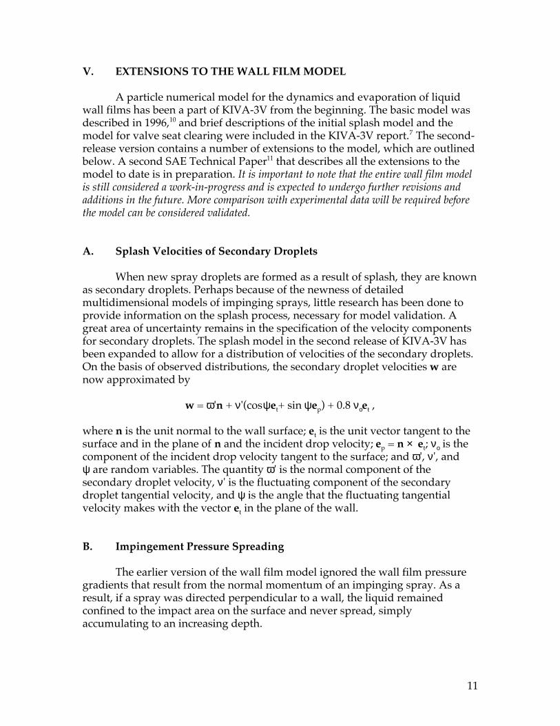
When new spray droplets are formed as a result of splash, they are knownas secondary droplets. Perhaps because of the newness of detailedmultidimensional models of impinging sprays, little research has been done toprovide information on the splash process, necessary for model validation. Agreat area of uncertainty remains in the specification of the velocity componentsfor secondary droplets. The splash model in the second release of KIVA-3V hasbeen expanded to allow for a distribution of velocities of the secondary droplets.On the basis of observed distributions, the secondary droplet velocities w arenow approximated by

w = ω'n + ν'(cos ψet+ sin ψep) + 0.8 νοet ,

where n is the unit normal to the wall surface; et is the unit vector tangent to thesurface and in the plane of n and the incident drop velocity; ep = n × et; νο is thecomponent of the incident drop velocity tangent to the surface; and ω', ν', andψ are random variables. The quantity ω' is the normal component of thesecondary droplet velocity, ν' is the fluctuating component of the secondarydroplet tangential velocity, and ψ is the angle that the fluctuating tangentialvelocity makes with the vector et in the plane of the wall.

B. Impingement Pressure Spreading

The earlier version of the wall film model ignored the wall film pressuregradients that result from the normal momentum of an impinging spray. As aresult, if a spray was directed perpendicular to a wall, the liquid remainedconfined to the impact area on the surface and never spread, simplyaccumulating to an increasing depth.

12

A model to remove this deficiency was added to KIVA-3V in the summerof 1997, and is embodied in a new subroutine named SPREAD. The approachmakes use of the surface pressure differences between the cell face that the liquidis impinging upon and the four abutting surface faces. These differences are thenused to accelerate wall film outward from an impingement site.

C. Particle Momentum and Energy

The calculation of the particle momentum has been expanded to includethe effect that the momentum of an impacting droplet has on the momentum offilm that is already on the wall, and vice versa. As part of this more accurateapproach, the UFILM-, VFILM-, and WFILM- arrays were replaced by UMOM-,VMOM-, and WMOM- arrays on 17 November 1997, as it became moreappropriate to work with the momenta.

If there is impingement in the present cycle, the pressure terms relating toimpingement pressure spreading (see Sec. V.B above) are calculated and used tomodify the momentum source term arrays before they are used in the filmvelocity calculation.

The new velocity of each film particle is based upon the wall shearstresses, the direction of gas flow relative to the wall, the mass source, themomentum source accumulated in subroutine SPLASH and modified insubroutine SPREAD, the momentum of the existing wall film, the mean filmtemperature, and the liquid viscosity at this temperature.

Also as part of the spray/wall interaction submodel, an energy termETERM has been introduced in the calculation of the wall particle temperature.ETERM approximates the impingement source term in the particle energyequation, multiplied by the film thickness and divided by twice the filmconductivity. When spray impinges on a wall film, the impingement mass mixeswith pre-existing film mass. Thus, ETERM for particles already on the wall thathave mixed with particles sticking to the wall during the current computationalcycle is different from ETERM for particles that have just stuck to the wall andmixed with pre-existing wall film particles. The new flag JUSTHIT is used todistinguish between the two types of particles.

ETERM is subtracted in the equation for the particle surface temperatureTPSURF, but we soon discovered that this could drive TPSURF negative.Analysis indicated that our traditional first guess for the new particletemperature, TPNEW = TPn, was no longer a good choice. A new equation forthe first guess for TPNEW, which eliminated the problem, uses ETERM as apositive quantity. The derivation of the new TPNEW equation is based upon theobservation that upon convergence, TPSURF ≈ TPn + 1. These changes were added22 May 1997.

13

D. Gravitational Terms

The effects of gravity on a wall film are considered minor in applicationsto operating engines. However, for comparison of KIVA-3V results with benchexperiments of impinging sprays and liquid film formation, the time scale is suchthat the effects may become nontrivial. To eliminate this area of uncertainty,gravitational terms were added to the wall film velocities on 14 April 1998.

E. Miscellaneous Corrections to the Wall Film Model

Several corrections have been made in the wall film model that are notdirectly related to the items discussed above.

¥ In the equation for DSIEP, the energy-coupling contribution in subroutineWALLFILM, the term HT was corrected to HTRANS on 25 April 1997.

¥ The particle mass term PARTE erroneously included a factor of FACSEC,which was removed 15 April 1997. PARTE is used in the calculation of thefilm thickness in subroutines LAWALL, PMOVTV, and SPLASH.

¥ A test was added to subroutine CLEAR on 2 April 1997 to ensure that a valveseat is cleared of all film when the valve closes. Previously, if the valve liftsuddenly went to zero from a value that was greater than the remaining filmthickness, the remaining film was left on the seat because there was nofurther opportunity to finish clearing it. When this situation arises, the addedtest sets the old value of the valve lift to 10Ð20, which will then force the finalclearing to occur.

¥ Tests were added 27 June 1997 to subroutine FILMSNAP to ensure that anadjustment of index I4P is made only if the particle is on the surface that isbeing snapped.

14

VI. OTHER NEW FEATURES

A. Split Injection

Today's increasingly sophisticated engine management systems areallowing designers to explore complex fuel-injection schedules. Whereas in thepast a single fuel-injection pulse per engine cycle was the norm for both gasolineand diesel engines, a number of current designs utilize more than one injectionpulse per engine cycle. Split injection is the designation for a schedule that hastwo or more distinct pulses. In some direct-injection gasoline engine designs, forexample, fuel is injected twiceÑan early pulse during the intake stroke and a latepulse during the compression stroke. There are now some diesel injectors thatdeliver a sequence of pulses.

The fuel-injection model in KIVA-3V has been expanded to allow splitinjection in addition to the ordinary single injection. A new input quantityNUMINJ specifies the number of injection pulses per engine cycle, which canrange from 1 to a maximum of LINJ, LINJ being a parameter in file comkiva.ithat currently has a value of 10. For each pulse, a set of the six input quantitiesT1INJ, TDINJ, CA1INJ, CADINJ, TSPMAS, and TNPARC are specified. Thuseach pulse has its own window, either in seconds or crank angle degrees, and itsown liquid mass and number of spray parcels.

B. Expanded Monitoring for Engine Calculations

Over the past several years I have been involved in modeling studies offuel-injected engines. As a diagnostic aid, I added a number of patches thatcalculated and wrote to output file OTAPE12 quantities related to the liquid andgaseous phases of the fuel and, for combustion runs, the energy balance data andemissions data. With the thought that this information might be useful to otherengine researchers, I have integrated these diagnostics into the program.

Subroutine NEWCYC calls a new subroutine named FUELMON if there isany fuel in the system. FUELMON monitors both the liquid and gaseous phasesof the fuel and considers the entire computing domain. It keeps track of themasses and current locations of wall film, entrained liquid and vapor. Four linesare written to the user's monitor and to file OTAPE12. Each line begins with aunique label that allows the user to edit the file and select a specific dataset forpostprocessing with data-analysis graphics software:

Line 1: crank angle; total fuel mass in the system; liquid mass entrained inregions 1Ð3; vapor mass entrained in regions 1Ð3.

15

Line 2: crank angle; fuel film mass on the valve surfaces, by surfacenumber, for up to 8 surfaces (4 valves).

Line 3: crank angle; fuel film mass on piston, liner, head, and walls of portregions 2 and 3.

Line 4: crank angle; entrained liquid mass lost out the left and right ports;film mass lost out the left and right ports; vapor mass lost out the left andright ports.

For combustion runs, the data printed by subroutine GLOBAL has beenexpanded to include energy balance data and emissions data:

The energy balance line contains the crank angle, the cumulative heatrelease from all chemical reactions, the cumulative change in total energyin the cylinder, the cumulative wall heat loss in the cylinder, and thecumulative pressure work done by the piston on the gas (all in ergs) aswell as the current total mass of pre-mixed fuel.

The emissions line contains the crank angle and the amounts of CO2, CO,and NO in the cylinder, in parts per million.

As in the original KIVA-3V, subroutine GLOBAL continues to printcumulative mass flux through open boundaries and cumulative mass fluxthrough each valve.

In subroutine MONITOR, the cylinder fuel injection data written to filedat.inject has been revised from that of the original KIVA-3V. With the thoughtthat subroutine FUELMON now comprehensively reports the fuel mass data,dat.inject now focuses on equivalence ratio information. There are now fourrather than three sorting bins: vapor mass with equivalence ratio less than 0.01,between 0.01 and 0.5, between 0.5 and 1.5, and greater than 1.5. Printed are thecrank angle, the total vapor mass in each of the four bins, and the total volumeassociated with each of the four bins.

C. Particle Evaporation Cutoff in Subroutine EVAP

A shortcoming of the numerical procedure in subroutine EVAP wasencountered, which occurred when the mass that it wanted to evaporate in aniteration was minuscule. As a result, the corresponding number of iterations(NIT) was in the millions and the computer time became enormous. A test toeliminate this pathological case was added 23 April 1998. If the mass to beevaporated is less than 10Ð6 the mass of the parcel, the iteration is terminated. Thecircumstance is transient and should automatically resolve itself over succeedingcycles.

16

D. Particle Energy Coupling Above Valves in Subroutine PCOUPL

Failures have occurred in port fuel-injection studies whereby, duringcoupling of particle specific internal energy to the gas field in cells immediatelyabove the top of an intake valve, the specific internal energy of the cell is drivennegative. When such failures have occurred, the volume of the cell has been quitesmall, a consequence of using the snapping technique to move the valves.

A test was added to subroutine PCOUPL on 9 May 1997 that checks to seewhether the proposed reduction of internal energy is greater than a quarter ofthe SIE of the cell. If so, the change is limited to that amount, and the remainderis taken out of the cell immediately above, which generally has a much largervolume and hence much more energy to offer than the affected cell.

Although this is clearly an ad hoc approach, it conserves specific internalenergy and has eliminated the problem. As a backup, the automatic restart of thecycle with a reduced time step (see Sec. II) is available if the SIE is ever drivennegative, from whatever cause, in subroutine PCOUPL.

17

VII. DATA STORAGE

Storage has been increased by the requirements of the automatic restart ofa cycle with a reduced time step, discussed in Sec. II. A new common block witharray names beginning with "RE" contains beginning-of-cycle values of thenecessary cell and vertex data. In addition, there are copies of most of the othercommon blocks.

There was a choice as to how to make copies of the common blocks. Onechoice would have been to continue to use the LOCR and LOCI functions thatdetermine the lengths of real and integer arrays. This would require the creationand maintenance of complete duplicate copies of each common block, line byline, with the names slightly changed. For example, every name could bepreceded by "RE." This approach would ensure that the duplicate commonsmatched the originals and were of the correct length.

The simpler approach that was chosen was to completely eliminate LOCRand LOCI and return to the use of parameter statements that specify the lengthsof the common blocks. Each duplicate common block contains a single array thatis given the dimension specified by the parameter statement. Changes were alsorequired in subroutines BEGIN, SORT, TAPERD, and TAPEWR. The user mustnow remember, however, to adjust the length of the parameter statement whenmaking changes to a common block.

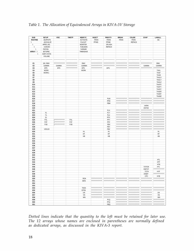
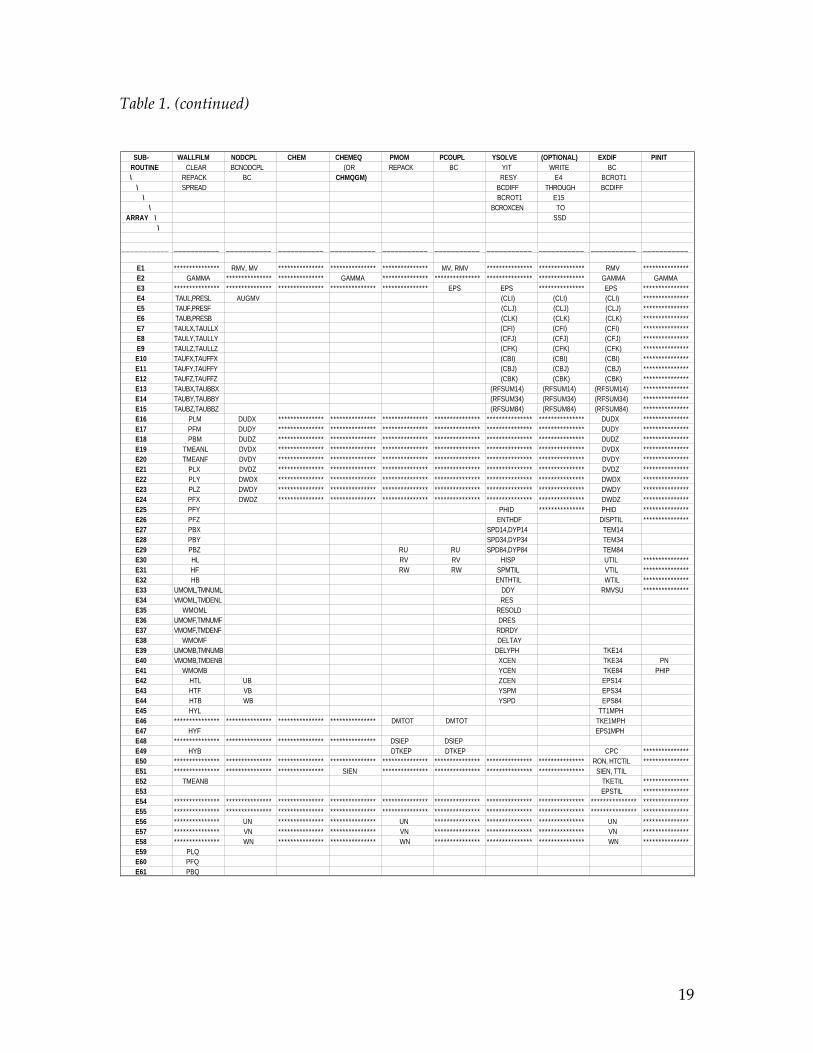
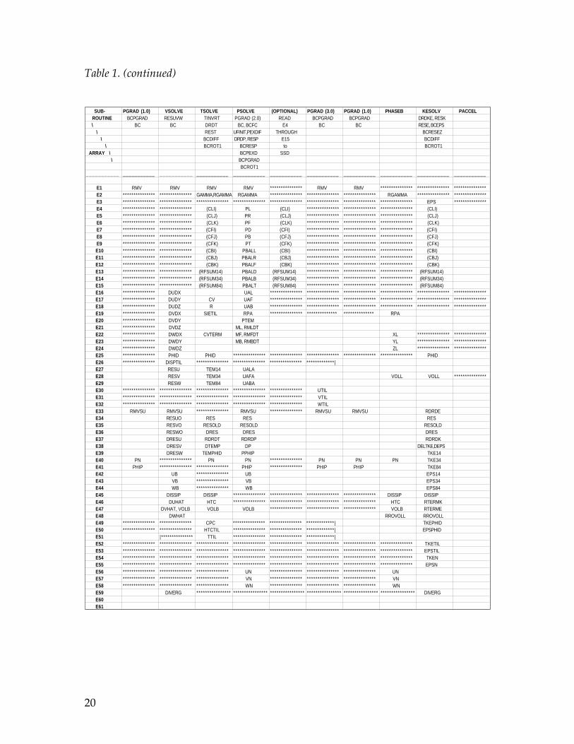
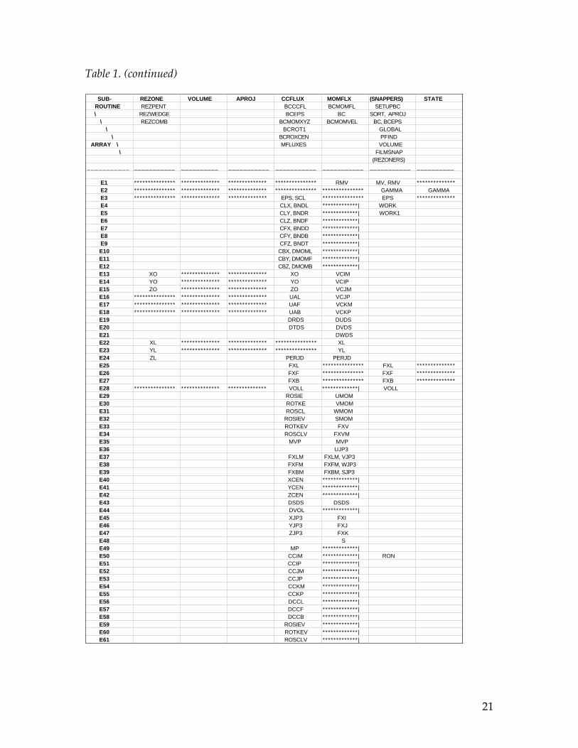
Table 1 shows the allocation of the equivalenced arrays in the new releaseversion of KIVA-3V. The differences between this and the table in Ref. 7 areprincipally in the wall film model, in which arrays with the name -FILM- havebeen replaced by arrays with the name -MOM-, and in the addition of the energysource terms for splashing droplets: PLQ, PFQ, and PBQ. These were discussedin Sec. V. The existing array RON is now also used in the four snappingsubroutines as part of the mass conservation improvement discussed in Sec. IV.B.There has been no increase in the number of equivalenced arrays.

18

Table 1. The Allocation of Equivalenced Arrays in KIVA-3V Storage

SUB- SETUP VISC TIMSTP NEWCYC INJECT PMOVTV BREAK COLIDE EVAP LAWALL ROUTINE ADJPISTN ACTIVATE FRAN FRAN FRAN FRAN BC \ ADJVALVE FULOUT PFIND PFIND REPACK \ APROJ, BC MONITOR SPLASH \ CONVEX FUELMON REPACK \ PISTON TAPEWR ARRAY \ SETUPBC TIMENSAVE \ SORT,STATE

VOLUME___________ ___________ ___________ ___________ ___________ ___________ ___________ ___________ ___________ ___________ ___________

E1 MV, RMV *************** *************** RMV *************** *************** *************** *************** *************** RMV E2 GAMMA GAMMA *************** GAMMA *************** *************** *************** *************** GAMMA GAMMA E3 EPS EPS *************** EPS *************** EPS *************** *************** *************** *************** E4 WORK WORK TAUL E5 WORK1 TAUF E6 TAUB E7 TAULX E8 TAULY E9 TAULZ E10 TAUFX E11 TAUFY E12 TAUFZ E13 TAUBX E14 TAUBY E15 TAUBZ E16 PLM *************** *************** *************** *************** E17 PFM *************** *************** *************** *************** E18 PBM *************** *************** *************** *************** E19 VAPM E20 ENTH0 E21 PLX *************** *************** *************** *************** E22 XL PLY *************** *************** *************** *************** E23 YL PLZ *************** *************** *************** *************** E24 ZL PFX *************** *************** *************** *************** E25 FXL |************** FXL PFY *************** *************** *************** *************** E26 FXF |************** FXF PFZ *************** *************** *************** *************** E27 FXB |************** FXB PBX *************** *************** *************** *************** E28 PBY *************** *************** *************** *************** E29 VSOLID PBZ *************** *************** *************** *************** E30 HL HL HL E31 HF HF HF E32 HB HB HB E33 E34 E35 E36 E37 E38 E39 E40 E41 E42 HTL E43 HTF E44 HTB E45 TOTCM HYL E46 DMTOT *************** E47 TOTH HYF E48 DSIEP *************** E49 CPC HYB E50 RON *************** *************** *************** *************** *************** *************** E51 SIEN *************** *************** *************** *************** *************** *************** E52 E53 E54 TKEN *************** *************** *************** *************** *************** *************** E55 EPSN *************** *************** *************** *************** *************** *************** E56 UN *************** *************** *************** *************** *************** UN E57 VN *************** *************** *************** *************** *************** VN E58 WN *************** *************** *************** *************** *************** WN E59 PLQ *************** *************** *************** *************** E60 PFQ *************** *************** *************** *************** E61 PBQ *************** *************** *************** ***************

Dotted lines indicate that the quantity to the left must be retained for later use.The 12 arrays whose names are enclosed in parentheses are normally definedas dedicated arrays, as discussed in the KIVA-3 report.

19

Table 1. (continued)

SUB- WALLFILM NODCPL CHEM CHEMEQ PMOM PCOUPL YSOLVE (OPTIONAL) EXDIF PINIT ROUTINE CLEAR BCNODCPL (OR REPACK BC YIT WRITE BC \ REPACK BC CHMQGM) RESY E4 BCROT1 \ SPREAD BCDIFF THROUGH BCDIFF \ BCROT1 E15 \ BCROXCEN TO ARRAY \ SSD \

___________ ___________ ___________ ___________ ___________ ___________ ___________ ___________ ___________ ___________ ___________

E1 *************** RMV, MV *************** *************** *************** MV, RMV *************** *************** RMV *************** E2 GAMMA *************** *************** GAMMA *************** *************** *************** *************** GAMMA GAMMA E3 *************** *************** *************** *************** *************** EPS EPS *************** EPS *************** E4 TAUL,PRESL AUGMV (CLI) (CLI) (CLI) *************** E5 TAUF,PRESF (CLJ) (CLJ) (CLJ) *************** E6 TAUB,PRESB (CLK) (CLK) (CLK) *************** E7 TAULX,TAULLX (CFI) (CFI) (CFI) *************** E8 TAULY,TAULLY (CFJ) (CFJ) (CFJ) *************** E9 TAULZ,TAULLZ (CFK) (CFK) (CFK) *************** E10 TAUFX,TAUFFX (CBI) (CBI) (CBI) *************** E11 TAUFY,TAUFFY (CBJ) (CBJ) (CBJ) *************** E12 TAUFZ,TAUFFZ (CBK) (CBK) (CBK) *************** E13 TAUBX,TAUBBX (RFSUM14) (RFSUM14) (RFSUM14) *************** E14 TAUBY,TAUBBY (RFSUM34) (RFSUM34) (RFSUM34) *************** E15 TAUBZ,TAUBBZ (RFSUM84) (RFSUM84) (RFSUM84) *************** E16 PLM DUDX *************** *************** *************** *************** *************** *************** DUDX *************** E17 PFM DUDY *************** *************** *************** *************** *************** *************** DUDY *************** E18 PBM DUDZ *************** *************** *************** *************** *************** *************** DUDZ *************** E19 TMEANL DVDX *************** *************** *************** *************** *************** *************** DVDX *************** E20 TMEANF DVDY *************** *************** *************** *************** *************** *************** DVDY *************** E21 PLX DVDZ *************** *************** *************** *************** *************** *************** DVDZ *************** E22 PLY DWDX *************** *************** *************** *************** *************** *************** DWDX *************** E23 PLZ DWDY *************** *************** *************** *************** *************** *************** DWDY *************** E24 PFX DWDZ *************** *************** *************** *************** *************** *************** DWDZ *************** E25 PFY PHID *************** PHID *************** E26 PFZ ENTHDF DISPTIL *************** E27 PBX SPD14,DYP14 TEM14 E28 PBY SPD34,DYP34 TEM34 E29 PBZ RU RU SPD84,DYP84 TEM84 E30 HL RV RV HISP UTIL *************** E31 HF RW RW SPMTIL VTIL *************** E32 HB ENTHTIL WTIL *************** E33 UMOML,TMNUML DDY RMVSU *************** E34 VMOML,TMDENL RES E35 WMOML RESOLD E36 UMOMF,TMNUMF DRES E37 VMOMF,TMDENF RDRDY E38 WMOMF DELTAY E39 UMOMB,TMNUMB DELYPH TKE14 E40 VMOMB,TMDENB XCEN TKE34 PN E41 WMOMB YCEN TKE84 PHIP E42 HTL UB ZCEN EPS14 E43 HTF VB YSPM EPS34 E44 HTB WB YSPD EPS84 E45 HYL TT1MPH E46 *************** *************** *************** *************** DMTOT DMTOT TKE1MPH E47 HYF EPS1MPH E48 *************** *************** *************** *************** DSIEP DSIEP E49 HYB DTKEP DTKEP CPC *************** E50 *************** *************** *************** *************** *************** *************** *************** *************** RON, HTCTIL *************** E51 *************** *************** *************** SIEN *************** *************** *************** *************** SIEN, TTIL E52 TMEANB TKETIL *************** E53 EPSTIL *************** E54 *************** *************** *************** *************** *************** *************** *************** *************** ******* ******** *************** E55 *************** *************** *************** *************** *************** *************** *************** *************** ******* ******** *************** E56 *************** UN *************** *************** UN *************** *************** *************** UN *************** E57 *************** VN *************** *************** VN *************** *************** *************** VN **** *********** E58 *************** WN *************** *************** WN *************** *************** *************** WN *************** E59 PLQ E60 PFQ E61 PBQ

20

Table 1. (continued)

SUB- PGRAD (1.0) VSOLVE TSOLVE PSOLVE (OPTIONAL) PGRAD (3.0) PGRAD (1.0) PHASEB KESOLV PACCEL ROUTINE BCPGRAD RESUVW TINVRT PGRAD (2.0) READ BCPGRAD BCPGRAD DRDKE, RESK \ BC BC DRDT BC, BCFC E4 BC BC RESE, BCEPS \ REST UFINIT,PEXDIF THROUGH BCRESEZ \ BCDIFF DRDP, RESP E15 BCDIFF \ BCROT1 BCRESP to BCROT1 ARRAY \ BCPEXD SSD \ BCPGRAD

BCROT1___________ ___________ ___________ ___________ ___________ ___________ ___________ ___________ ___________ ___________ ___________

E1 RMV RMV RMV RMV *************** RMV RMV *************** *************** *************** E2 *************** *************** GAMMA,RGAMMA RGAMMA *************** *************** *************** RGAMMA *************** *************** E3 *************** *************** *************** *************** *************** *************** *************** *************** EPS *************** E4 *************** *************** (CLI) PL (CLI) *************** *************** *************** (CLI) E5 *************** *************** (CLJ) PR (CLJ) *************** *************** *************** (CLJ) E6 *************** *************** (CLK) PF (CLK) *************** *************** *************** (CLK) E7 *************** *************** (CFI) PD (CFI) *************** *************** *************** (CFI) E8 *************** *************** (CFJ) PB (CFJ) *************** *************** *************** (CFJ) E9 *************** *************** (CFK) PT (CFK) *************** *************** *************** (CFK) E10 *************** *************** (CBI) PBALL (CBI) *************** *************** *************** (CBI) E11 *************** *************** (CBJ) PBALR (CBJ) *************** *************** *************** (CBJ) E12 *************** *************** (CBK) PBALF (CBK) *************** *************** *************** (CBK) E13 *************** *************** (RFSUM14) PBALD (RFSUM14) *************** *************** *************** (RFSUM14) E14 *************** *************** (RFSUM34) PBALB (RFSUM34) *************** *************** *************** (RFSUM34) E15 *************** *************** (RFSUM84) PBALT (RFSUM84) *************** *************** *************** (RFSUM84) E16 *************** DUDX UAL *************** *************** *************** *************** *************** *************** E17 *************** DUDY CV UAF *************** *************** *************** *************** *************** *************** E18 *************** DUDZ R UAB *************** *************** *************** *************** *************** *************** E19 *************** DVDX SIETIL RPA *************** ************** ************** RPA E20 *************** DVDY PTEM E21 *************** DVDZ ML, RMLDT E22 *************** DWDX CVTERM MF, RMFDT XL *************** *************** E23 *************** DWDY MB, RMBDT YL *************** *************** E24 *************** DWDZ ZL *************** *************** E25 *************** PHID PHID *************** *************** *************** *************** *************** PHID E26 *************** DISPTIL *************** *************** *************** *************| E27 RESU TEM14 UALA E28 RESV TEM34 UAFA VOLL VOLL *************** E29 RESW TEM84 UABA E30 *************** *************** *************** *************** *************** UTIL E31 *************** *************** *************** *************** *************** VTIL E32 *************** *************** *************** *************** *************** WTIL E33 RMVSU RMVSU *************** RMVSU *************** RMVSU RMVSU RDRDE E34 RESUO RES RES RES E35 RESVO RESOLD RESOLD RESOLD E36 RESWO DRES DRES DRES E37 DRESU RDRDT RDRDP RDRDK E38 DRESV DTEMP DP DELTKE,DEPS E39 DRESW TEMPHID PPHIP TKE14 E40 PN *************** PN PN *************** PN PN PN TKE34 E41 PHIP *************** *************** PHIP *************** PHIP PHIP TKE84 E42 UB *************** UB EPS14 E43 VB *************** VB EPS34 E44 WB *************** WB EPS84 E45 DISSIP DISSIP *************** *************** *************** *************** DISSIP DISSIP E46 DUHAT HTC *************** *************** *************** *************** HTC RTERMK E47 DVHAT, VOLB VOLB VOLB *************** *************** *************** VOLB RTERME E48 DWHAT RROVOLL RROVOLL E49 *************** *************** CPC *************** *************** *************| TKEPHID E50 *************** *************** HTCTIL *************** *************** *************| EPSPHID E51 |*************** TTIL *************** *************** *************| E52 *************** *************** *************** *************** *************** *************** *************** *************** TKETIL E53 *************** *************** *************** *************** *************** *************** *************** *************** EPSTIL E54 *************** *************** *************** *************** *************** *************** *************** *************** TKEN E55 *************** *************** *************** *************** *************** *************** *************** *************** EPSN E56 *************** *************** *************** UN *************** *************** *************** UN E57 *************** *************** *************** VN *************** *************** *************** VN E58 *************** *************** *************** WN *************** *************** *************** WN E59 DIVERG **************** **************** **************** **************** **************** **************** DIVERG E60 E61

21

Table 1. (continued)

SUB- REZONE VOLUME APROJ CCFLUX MOMFLX (SNAPPERS) STATE ROUTINE REZPENT BCCCFL BCMOMFL SETUPBC \ REZWEDGE BCEPS BC SORT, APROJ \ REZCOMB BCMOMXYZ BCMOMVEL BC, BCEPS \ BCROT1 GLOBAL \ BCROXCEN PFIND ARRAY \ MFLUXES VOLUME \ FILMSNAP

(REZONERS)___________ ___________ __________ ___________ ___________ ___________ ___________ __________

E1 *************** ************** ************** *************** RMV MV, RMV ************** E2 *************** ************** ************** *************** *************** GAMMA GAMMA E3 *************** ************** ************** EPS, SCL *************** EPS ************** E4 CLX, BNDL *************| WORK E5 CLY, BNDR *************| WORK1 E6 CLZ, BNDF *************| E7 CFX, BNDD *************| E8 CFY, BNDB *************| E9 CFZ, BNDT *************| E10 CBX, DMOML *************| E11 CBY, DMOMF *************| E12 CBZ, DMOMB *************| E13 XO ************** ************** XO VCIM E14 YO ************** ************** YO VCIP E15 ZO ************** ************** ZO VCJM E16 *************** ************** ************** UAL VCJP E17 *************** ************** ************** UAF VCKM E18 *************** ************** ************** UAB VCKP E19 DRDS DUDS E20 DTDS DVDS E21 DWDS E22 XL ************** ************** *************** XL E23 YL ************** ************** *************** YL E24 ZL PERJD PERJD E25 FXL *************** FXL ************** E26 FXF *************** FXF ************** E27 FXB *************** FXB ************** E28 *************** ************** ************** VOLL *************| VOLL E29 ROSIE UMOM E30 ROTKE VMOM E31 ROSCL WMOM E32 ROSIEV SMOM E33 ROTKEV FXV E34 ROSCLV FXVM E35 MVP MVP E36 UJP3 E37 FXLM FXLM, VJP3 E38 FXFM FXFM, WJP3 E39 FXBM FXBM, SJP3 E40 XCEN *************| E41 YCEN *************| E42 ZCEN *************| E43 DSDS DSDS E44 DVOL *************| E45 XJP3 FXI E46 YJP3 FXJ E47 ZJP3 FXK E48 S E49 MP *************| E50 CCIM *************| RON E51 CCIP *************| E52 CCJM *************| E53 CCJP *************| E54 CCKM *************| E55 CCKP *************| E56 DCCL *************| E57 DCCF *************| E58 DCCB *************| E59 ROSIEV *************| E60 ROTKEV *************| E61 ROSCLV *************|

22

VIII. ADDITIONS TO FILE ITAPE5

It is with some reluctance that I have added quantities to input fileITAPE5, but it was necessary in order to properly support two new KIVA-3Vfeatures described above:

1) DEACT, which controls port deactivation/reactivation, described inSec. III, and

2) NUMINJ, the number of injection pulses, described in Sec. VI.A. Thereare NUMINJ sets of the following six quantities: T1INJ, TDINJ, CA1INJ,CADINJ, TSPMAS, and TNPARC. Note that there is a local rearrangement of theinjection data on file ITAPE5 to make these six quantities contiguous.

23

IX. ADDITIONS TO K3PREP

Several new optional features have been added to the parametric gridgenerator K3PREP, which result in additional lines in the IPREP file.

A. Rounding of Runner Segments

The intake and exhaust regions in the four examples of valved engines inthe KIVA-3V report7 are composed of valve ports and attached single-blockrunners. Shaping of the blocks is performed by subroutines VALVPORT,RUNNER, and SIAMESE. In all these examples, the runners are a single blockthat extends from a valve port to a pressure boundary, and represent theportions of the intake and exhaust passages that lie within the cylinder headcasting. Although this block definition is adequate for the sample geometries,other engine designs require much more complex runners, with such features aslong curved shapes, helical ports, and bifurcations. Also, it may be desirable toinclude a much greater portion of the induction system.

The creation of a helical intake port, as one example, requires a largenumber of blocks to achieve a smooth shape. Rounding the edges of these addedrunner segments is beyond the scope of subroutine RUNNER, and thus a newsubroutine named ROUND has been added to address this need.

¥ NROUND (format A10,I5) is the number of runner segments to be rounded. IfNROUND > 0, (NROUND) lines follow, each of which contains:

¥ N, NORIENT, RAD1, RAD2 (format 2I4,2F8.3), which says: Round the solidedges of runner extension block N. NORIENT specifies the logical orientationof flow through the segment, and RAD1 and RAD2 specify the radii ofcurvature of the solid edges. In the following chart L, R, F, D, B, and T havetheir usual KIVA meanings of left, right, front, derriere, bottom, and top:

NORIENT: RAD1: RAD2:

1 = L ↔ R FB & FT DB & DT2 = F ↔ D LB & LT RB & RT3 = B ↔ T LF & RF LD & RD

The NROUND command lines follow NSIAMESE and precede NPATCHin the IPREP file.

24

B. Valve Guides

Previously there was no provision in K3PREP to model valve guideintrusion into a valve port. Subroutine VALGUIDE has been added to shape anddeactivate specified cells to represent valve guides.

¥ NVGUIDE (format A10,I5) is the number of valve guides to be modeled. IfNVGUIDE > 0, (NVGUIDE) lines follow, each of which contains:

¥ N, NXYGUIDE, NZGUIDE, XSHIFT, YSHIFT, RADGUIDE, ZTOBOT (format3I4,4F8.3) says: Create a valve guide in valve port N that is NXYGUIDE cellswide by NZGUIDE cells high, and is centered at (XSHIFT,YSHIFT), where(XSHIFT,YSHIFT) is the x and y translation of the blocks. The guide has aradius of RADGUIDE cm, and its lower edge is at ZTOBOT cm up from theedge of the valve seat (bottom of block N).

The NVGUIDE command lines follow NPENTXY and precedeNVALVPORT in the IPREP file.

How accurately the user can represent a valve guide depends on theparticular geometry. The resulting shapes of the cells around the guide are themost satisfactory when the base of the guide extends some distance into the port.However, engine designers try to make guides as nonintrusive as possible,balancing the requirement for good valve stem support with the need tominimize flow blockage. If the base of the valve guide intersects the outer radiusof the port, or worse, if it lies above the port, it may be difficult or impossible toachieve satisfactory zoning because cell edges get collapsed on top of oneanother. This is one of the difficulties of working with a structured mesh. If anaccurate representation of a valve guide produces an unacceptable mesh in theport, the user should either sacrifice some accuracy by moving the bottom of theguide down a bit, or forego the valve guide option entirely.

C. Cell-Face Boundary Conditions for Valve Stems

If you are generating a vertical-valve mesh with curved valve ports andare using the original IPREP for the vertical-valve example in Ref. 7 as a pattern,you will need to change the boundary condition for the left, right, derriere (andfront if full-circle mesh) faces of the valve stems from 2.0 (SOLID) to 1.0(MOVING), for blocks 23, 24, 25, and 39, 40, 41, along with specifying theappropriate IDFACE (4 or 2). Failure to do this will result in crooked valvestems, which arise in subroutine VALVPORT.

The original vertical valve mesh was created and in use a year beforesubroutine VALVPORT was written for the first canted-valve mesh. The meshwas to be used in a port fuel-injection study with our particle model for liquid

25

wall films. For the film to move properly on the intake valve stems, it wasnecessary to make the left, right, front, and derriere faces on the stems MOVINGinstead of SOLID. Note that KIVA-3V never actually moves the stem vertices,which ensures that the zoning never changes around the stem, but the currentvelocity of the valve is the wall velocity needed in the wall film model.

By the time I wrote subroutine VALVPORT, I was thinking in terms ofvalve stems being MOVING. Note that in the Do 260 loop of the subroutinethere is an ELSEIF statement that includes a test on IDFACE(I4) ≥ 2. The result ofthis test is that valve stems are left where they belong, but it also assumes thatthe valve stem is MOVING, with a correct IDFACE (2, 4, ...). An IDFACE of Ð1will allow the (x,y) coordinates of the valve stem to change and result in itsbecoming crooked.

The cell-face boundary condition problem went undiscovered until I firstcurved the ports in the vertical-valve example.

D. Miscellaneous Changes and Notes

¥ A seventh column named IFIXED has been appended to the lines of block-reshaping commands read by subroutine RESHAPEB. Normally, IFIXED = 0;it is set to 1 only when reshaping a cylinder to match the outline of a bowlblock below it. An example is shown in Sec. IX.E below.

¥ The earlier K3PREP could require user patches in subroutine RESHAPEB if astraight line was to be enforced across x = 0 or y = 0. The need for a patch hasbeen eliminated by the addition of two flags in the IPREP file. If RESHAPE >0, the two integer flags STRAIGHTX0 and STRAIGHTY0, each with format(A10,I5), must now be inserted at the end of the list of reshaping commands.If STRAIGHTX0 = 1, the mesh will have a straight line through x = 0, and ifSTRAIGHTY0 = 1, the mesh will have a straight line through y = 0.

¥ XBAND, YBAND, and ZBAND have been added to the IPREP file, followingthe PLOTMESH line. These have the same purpose as the quantities of thesame name in K3POST (see pages 69Ð70 in Ref. 7), which is to control thethickness of the band considered in the plot subroutines ZONPLTX,ZONPLTY, and ZONPLTZ.

¥ Subroutine ZONHIDE now automatically makes a mirror-image plot acrossyÊ= 0 for half-circle symmetry meshes, provided there is adequate storage(NVERTS*2 ≤ NV) for the reflected vertex and cell-face data.

26

E. Diesel Engine Grid with Vertical Valves and a Piston Bowl

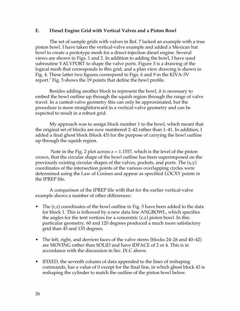
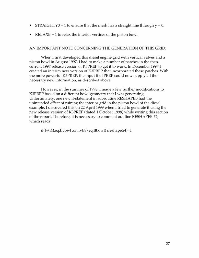
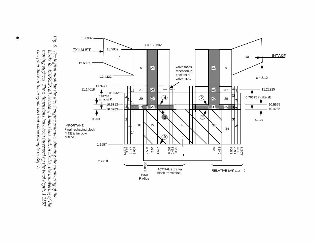
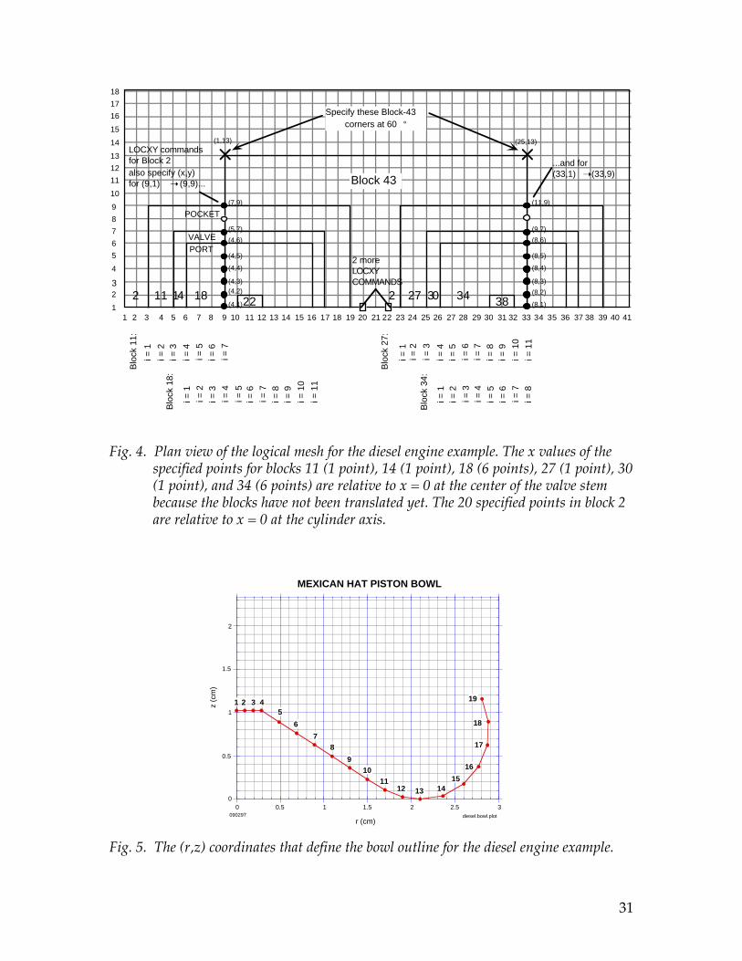
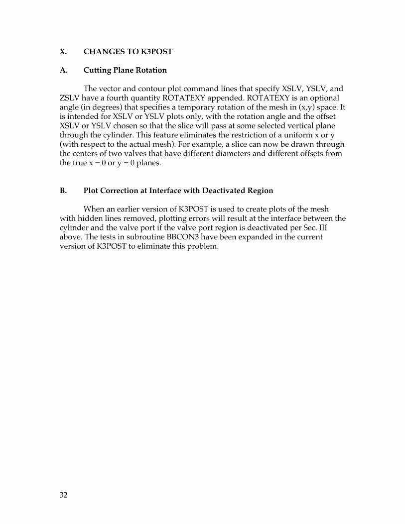
The set of sample grids with valves in Ref. 7 lacked an example with a truepiston bowl. I have taken the vertical-valve example and added a Mexican hatbowl to create a prototype mesh for a direct-injection diesel engine. Severalviews are shown in Figs. 1 and 2. In addition to adding the bowl, I have usedsubroutine VALVPORT to shape the valve ports. Figure 3 is a drawing of thelogical mesh that corresponds to this grid, and a plan view drawing is shown inFig. 4. These latter two figures correspond to Figs. 6 and 9 in the KIVA-3Vreport.7 Fig. 5 shows the 19 points that define the bowl profile.

Besides adding another block to represent the bowl, it is necessary toembed the bowl outline up through the squish region through the range of valvetravel. In a canted-valve geometry this can only be approximated, but theprocedure is more straightforward in a vertical-valve geometry and can beexpected to result in a robust grid.

My approach was to assign block number 1 to the bowl, which meant thatthe original set of blocks are now numbered 2Ð42 rather than 1Ð41. In addition, Iadded a final ghost block (block 43) for the purpose of carrying the bowl outlineup through the squish region.

Note in the Fig. 2 plot across z = 1.1557, which is the level of the pistoncrown, that the circular shape of the bowl outline has been superimposed on thepreviously existing circular shapes of the valves, pockets, and ports. The (x,y)coordinates of the intersection points of the various overlapping circles weredetermined using the Law of Cosines and appear as specified LOCXY points inthe IPREP file.

A comparison of the IPREP file with that for the earlier vertical-valveexample shows a number of other differences:

¥ The (r,z) coordinates of the bowl outline in Fig. 5 have been added to the datafor block 1. This is followed by a new data line ANGBOWL, which specifiesthe angles for the tent vertices for a concentric (r,z) piston bowl. In thisparticular geometry, 60 and 120 degrees produced a much more satisfactorygrid than 45 and 135 degrees.

¥ The left, right, and derriere faces of the valve stems (blocks 24Ð26 and 40Ð42)are MOVING rather than SOLID and have IDFACE of 2 or 4. This is inaccordance with the discussion in Sec. IX.C above.

¥ IFIXED, the seventh column of data appended to the lines of reshapingcommands, has a value of 0 except for the final line, in which ghost block 43 isreshaping the cylinder to match the outline of the piston bowl below.

27

¥ STRAIGHTY0 = 1 to ensure that the mesh has a straight line through y = 0.

¥ RELAXB = 1 to relax the interior vertices of the piston bowl.

AN IMPORTANT NOTE CONCERNING THE GENERATION OF THIS GRID:

When I first developed this diesel engine grid with vertical valves and apiston bowl in August 1997, I had to make a number of patches in the then-current 1997 release version of K3PREP to get it to work. In December 1997 Icreated an interim new version of K3PREP that incorporated these patches. Withthe more powerful K3PREP, the input file IPREP could now supply all thenecessary new information, as described above.

However, in the summer of 1998, I made a few further modifications toK3PREP based on a different bowl geometry that I was generating.Unfortunately, one new if-statement in subroutine RESHAPEB had theunintended effect of ruining the interior grid in the piston bowl of the dieselexample. I discovered this on 22 April 1999 when I tried to generate it using thenew release version of K3PREP (dated 1 October 1998) while writing this sectionof the report. Therefore, it is necessary to comment out line RESHAPEB.72,which reads:

if(fv(i4).eq.flbowl .or. fv(i8).eq.flbowl) ireshape(i4)=1

28

Fig. 1. Half-circle mesh for the direct-injection diesel engine example with two verticalvalves and a Mexican hat piston bowl. The mesh contains 24,013 grid points.

29

Fig. 2. Top: the diesel engine mesh through the y = 0 symmetry plane. Bottom: planview through the squish region.

30

RELATIVE to ¤ at x = 0ACTUAL ± x afterblock translation

38

16.6332

EXHAUST

13.6332

15.5832

7

12.4332

11.3492

10.93320.81788exhaust lift

10.5313

10.3283

0.203

IMPORTANT:Final reshaping block(#43) is for bowloutline.

1.1557

z = 15.0332

6 26

517 21 25

413

1620

3 1215 19 23

18

2

11

14

24

22

3

4

valve facesrecessed inpockets atvalve TDC

2

1

4334

30

27

39 35 3128

29

3236

37

942

41

10

338 11.22225

0.79375 intake lift

10.555510.4285

0.127

INTAKE

z = 0.0

11.14618

0

40

4.12

753.

953.

767

3.60

9

2.53

3

2.10

1.66

7

0.59

10.

433

0.25 0.0

0.43

3

1.50

91.

667

1.85

2.02

750

1

2.80

68

BowlRadius

x = 8.10

Fig. 3. The logical m

esh for the diesel engine example, show

ing the numbering of the

blocks for K3P

RE

P, all necessary dim

ensions and, in circles, the numbering of the

moving surfaces. T

he z dimensions have been increased by the bow

l depth, 1.1557cm

, from those in the original vertical-valve exam

ple in Ref. 7.

31

23

4

5

6

7

8

9

10

11

12

13

14

15

16

17

18

11 54 6 7 8 9 10 11 12 1314 15 16 17 18 19 20 2122 2324 25 26 272 3 28 29 34 3536 3730 31 32 33 38 4041391 54 6 7 8 92 3 1310 11 12 14 15 16 17 18 19 20 21 22 23 24 25 26 27 28 29 30 31 32 33 34 35 36 37 38 39 40 41

POCKET

VALVEPORT

Specify these Block-43corners at 60 °

LOCXY commandsfor Block 2also specify (x,y)for (9,1) ➝ (9,9)...

...and for(33,1) ➝ (33,9)

Block 43

2 14 18 22 2 27 30 34 3811

(7,9)

(5,7)

(4,6)

(4,5)

(4,4)

(4,3)(4,2)

(4,1)

(11,9)

(9,7)

(8,6)

(8,5)

(8,4)

(8,3)

(8,2)

(8,1)

2 moreLOCXYCOMMANDS

(1,13) (25,13)B

lock

11:

i = 1

i = 2

i = 4

i = 5

i = 6

i = 3

i = 7

Blo

ck 1

8:

i = 8

i = 9

i = 1

0

i = 1

i = 2

i = 4

i = 5

i = 6

i = 3

i = 7

i = 1

1

Blo

ck 2

7:

i = 8

i = 9

i = 1

0

i = 1

i = 2

i = 4

i = 5

i = 6

i = 3

i = 7

Blo

ck 3

4:

i = 1

i = 2

i = 4

i = 5

i = 6

i = 3

i = 7

i = 1

1i =

8

Fig. 4. Plan view of the logical mesh for the diesel engine example. The x values of thespecified points for blocks 11 (1 point), 14 (1 point), 18 (6 points), 27 (1 point), 30(1 point), and 34 (6 points) are relative to x = 0 at the center of the valve stembecause the blocks have not been translated yet. The 20 specified points in block 2are relative to x = 0 at the cylinder axis.

Fig. 5. The (r,z) coordinates that define the bowl outline for the diesel engine example.

0

0.5

1

1.5

2

0 0.5 1 1.5 2 2.5 3

MEXICAN HAT PISTON BOWL

z (c

m)

r (cm)

1 2 3 45

6

78

910

1112 13 14

15

16

17

18

19

diesel.bowl.plot090297

32

X. CHANGES TO K3POST

A. Cutting Plane Rotation

The vector and contour plot command lines that specify XSLV, YSLV, andZSLV have a fourth quantity ROTATEXY appended. ROTATEXY is an optionalangle (in degrees) that specifies a temporary rotation of the mesh in (x,y) space. Itis intended for XSLV or YSLV plots only, with the rotation angle and the offsetXSLV or YSLV chosen so that the slice will pass at some selected vertical planethrough the cylinder. This feature eliminates the restriction of a uniform x or y(with respect to the actual mesh). For example, a slice can now be drawn throughthe centers of two valves that have different diameters and different offsets fromthe true x = 0 or y = 0 planes.

B. Plot Correction at Interface with Deactivated Region

When an earlier version of K3POST is used to create plots of the meshwith hidden lines removed, plotting errors will result at the interface between thecylinder and the valve port if the valve port region is deactivated per Sec. IIIabove. The tests in subroutine BBCON3 have been expanded in the currentversion of K3POST to eliminate this problem.

33

ACKNOWLEDGMENTS

I wish to thank Peter O'Rourke for his continuing collaboration on the wallfilm model and Norman Johnson for his time and patience in discussing manyKIVA-3V-related topics. Norman has also maintained the KIVA information onour website and has made the reports of Refs. 5Ð7 available electronically. Iwould also like to acknowledge the many useful interactions that I have hadwith the worldwide KIVA user community and the inspiration that thecommunity has been to me. These interactions have resulted in a number ofimprovements and corrections to KIVA-3V.

Finally, I thank Margaret Findley once again for creating a number of thefigures and for her careful work in preparing my reports for publication.

34

REFERENCES

1. A. A. Amsden, T. D. Butler, P. J. O'Rourke, and J. D. Ramshaw, "KIVA: AComprehensive Model for 2-D and 3-D Engine Simulations," SAETechnical Paper 850554 (1985).

2. A. A. Amsden, J. D. Ramshaw, P. J. O'Rourke, and J. K. Dukowicz, "KIVA:A Computer Program for Two- and Three-Dimensional Fluid Flows withChemical Reactions and Fuel Sprays," Los Alamos National Laboratoryreport LA-10245-MS (February 1985).

3 A. A. Amsden, J. D. Ramshaw, L. D. Cloutman, and P. J. O'Rourke,"Improvements and Extensions to the KIVA Computer Program," LosAlamos National Laboratory report LA-10534-MS (October 1985).

4. A. A. Amsden, T. D. Butler, and P. J. O'Rourke, "The KIVA-II ComputerProgram for Transient Multidimensional Chemically Reactive Flows withSprays," SAE Technical Paper 872072 (1987).

5. A. A. Amsden, P. J. O'Rourke, and T. D. Butler, "KIVA-II: A ComputerProgram for Chemically Reactive Flows with Sprays," Los AlamosNational Laboratory report LA-11560-MS (May 1989).

6. A. A. Amsden, "KIVA-3: A KIVA Program with Block-Structured Mesh forComplex Geometries," Los Alamos National Laboratory report LA-12503-MS (March 1993).

7. A. A. Amsden, "KIVA-3V: A Block-Structured KIVA Program for Engineswith Vertical or Canted Valves," Los Alamos National Laboratory reportLA-13313-MS (July 1997).

8. A. B. Liu, D. Mather, and R. D. Reitz, "Modeling the Effects of Drop Dragand Breakup on Fuel Sprays," SAE Technical Paper 930072 (1993).

9. P. J. O'Rourke and A. A. Amsden, "The TAB Method for NumericalCalculation of Spray Droplet Breakup," SAE Technical Paper 872089(1987).

10. P. J. O'Rourke and A. A. Amsden, "A Particle Numerical Model for WallFilm Dynamics in Port-Injected Engines," SAE Technical Paper 961961(1996).

11. P. J. O'Rourke and A. A. Amsden, "A Spray/Wall Interaction Submodelfor the KIVA-3 Wall Film Model," SAE Technical Paper (in preparation).