Kinodynamic Randomized Rearrangement Planningvia Dynamic Transitions Between Statically Stable States

Joshua A. Haustein∗, Jennifer King†, Siddhartha S. Srinivasa†, Tamim Asfour∗∗Karlsruhe Institute of Technology(KIT) † Carnegie Mellon University(CMU)

joshua.haustein@gmail.com, asfour@kit.edu, {jeking,siddh}@cs.cmu.edu

Abstract—In this work we present a fast kinodynamicRRT-planner that uses dynamic nonprehensile actions torearrange cluttered environments. In contrast to manyprevious works, the presented planner is not restrictedto quasi-static interactions and monotonicity. Instead theresults of dynamic robot actions are predicted using a blackbox physics model. Given a general set of primitive actionsand a physics model, the planner randomly explores theconfiguration space of the environment to find a sequenceof actions that transform the environment into some goalconfiguration.

In contrast to a naive kinodynamic RRT-planner we showthat we can exploit the physical fact that in an environmentwith friction any object eventually comes to rest. Thisallows a search on the configuration space rather than thestate space, reducing the dimension of the search spaceby a factor of two without restricting us to non-dynamicinteractions.

We compare our algorithm against a naive kinodynamicRRT-planner and show that on a variety of environments wecan achieve a higher planning success rate given a restrictedtime budget for planning.

I. Introduction

We study the rearrangement planning problem [6, 9,11, 17, 21] where a robot must manipulate severalobjects in clutter to achieve a goal. Rearrangementof clutter can significantly increase the success rateof manipulation tasks [9, 11] and perception [18, 24],and is increasingly significant in unstructured humanenvironments such as homes, workplaces, disaster sitesand shared workcells in factories.

Consider a robot clearing a set of toys from a table.As shown in Fig. 1, the table is cluttered with objects.The robot’s goal is to move the green box into acrate, weaving through clutter. Early works focusedon finding a sequence of pick-and-place actions thatmoved clutter aside and eventually the target to itsgoal [22]. Recent work has shown that nonprehensileactions such as pushing, pulling, sliding, and sweeping,enable faster and better solutions, with higher successrates [5, 7, 16].

The problem of rearrangement planning has beenshown to be NP-hard [25]. Previous works have usedheuristics such as monotonicity to keep the problemtractable [8, 22]. Nonprehensile interactions have beenmodeled as motion primitives under the quasi-static as-sumption that any inertial forces can be neglected dueto frictional forces [6, 7]. While there exist analyticalquasi-static pushing models [10, 12, 15] that allow a fastto compute prediction of the object’s behavior duringa push, the actions and objects this can be applied toare limited.

We are interested in overcoming these limitations andpresent a planner that utilizes dynamic nonprehensile

Fig. 1. A robot clearing a table. First, the robot’s task is to pushthe green box to a goal region(green circle) inside of a crate (a)-(g).Afterwards, the robot is supposed to push the green ball to the samearea (h)-(p). The bottom row shows the total displacements for eachtrajectory. The trajectories were generated for a floating end-effectorin a 2D-workspace.

actions to rearrange clutter without being restricted tomonotonicity. In our example, after the robot pushesthe box into the crate its goal is to put a ball intothe crate. In this case the robot must reason about thedynamic behavior of the ball as the ball might fall offthe table otherwise.

The recent increasing availability of fast dynamicrigid body physics models [1–4] allows modeling dy-namic interactions between a robot and the objects inits environment in planning algorithms [27, 28]. Underthe quasi-static assumption the rearrangement problemcan be formulated as a search for a sequence of robotactions on the joint configuration space of the robot andeach movable object in the environment. In contrast,a costly consequence of dynamic interactions is thatthe search space becomes the full state space of theenvironment, containing both the configuration andvelocity of each object and the robot, doubling thedimension of the search space.

(a) Labyrinth maze1 (b) Pool billard (c) Bouldering2 (d) Mini golf3

Fig. 2. Examples for dynamic actions between statically stable states utilized by humans.

Our insight is that by choosing dynamic actions thatresult in statically stable states, e.g. the environmentcomes to rest after each action, we can search onthe lower dimensional configuration space. Considera bartender sliding a beer bottle to a customer or achild kicking a soccer ball. In both cases, in absence ofany external forces other than gravity, the manipulatedobject eventually comes to rest due to friction. In manyactivities humans follow a similar approach by transi-tioning dynamically from one static state into anotherstatic state (see Fig. 2).

We contribute by formulating the rearrangementproblem as a search for dynamic transitions betweenstatically stable states in the joint configuration space.We show that we can utilize a kinodynamic RRT [14]to solve this search problem. The planner explores theconfiguration space by randomly sampling dynamicnonprehensile actions and utilizing a dynamic blackbox physics model to predict the actions’ outcomes.To guarantee statically stable states, we require theenvironment for each action to come to rest after aduration Tmax. We compare our algorithm to a full-dynamic search and show that with a reasonable choicefor Tmax we can achieve a better planning time even forchallenging environments. As a result we show thatthe probability for our planner to find a solution in arestricted time frame is higher compared to a dynamicplanner.

This work is structured in the following way. InSec. II we formalize the problem of rearrangementplanning. Our algorithm is presented in Sec. III andour experiments are described in Sec. IV. In Sec. IV-Cwe present our results in simulation and on a robot.Finally, we discuss limitations and future work in Sec. Vand finish in Sec. VI with a conclusion.

II. The Rearrangement Planning Problem

A. Terminology

In our work an environment E contains a robot R, atarget object T, M movable objects the robot is allowedto manipulate and a set S of static obstacles the robotmust not collide with.

We denote the state of movable object i ∈ {1, . . . , M}as xi = (qi, qi) ∈ X i, where qi is the object’s configura-tion and qi its velocity. Analogously, we denote the state

1Image: Labyrinth of Failure by Kim Navarre from Brooklyn, NYpublished on http://commons.wikimedia.org/wiki/File:Labyrinth_of_Failure.jpg, accessed 2014

2Image: Hueco Tanks Bouldering by Surfsupusa at EnglishWikipedia published on http://commons.wikimedia.org/wiki/File:Hueco_Tanks_Bouldering.jpg, accessed 2014

3Image: Bulltoftaparken, Minigolfbanan by User Jorchr onsv.wikipedia published on http://commons.wikimedia.org/wiki/File:Bulltoftaparken,_Minigolfbanan.jpg, accessed 2014

space of the target object as X T and the robot as X R.We describe the state space of the environment X E asthe Cartesian product X E = X R×X T ×X 1× . . .×XM

of the state spaces of all objects in the scene and therobot. We define the free state space X E

f ree ⊆ XE as the

set of states in which no objects are penetrating andthe robot is not in collision with any static obstaclein S . Note that this definition specifically allows formovable objects, the target and the robot to be incontact with each other. Furthermore, contact betweenmovable objects or the target and static obstacles isincluded.

Throughout this work we denote the manifold CE ={(q, q) ∈ X E

f ree | q = 0} as the environment’s statically

stable free state space, where every object and the robotare at rest. Note that this is the free configurationspace. Likewise, let CT , CR and C i denote the staticallystable free state spaces for the target, the robot and allmovable objects i ∈ {1, ..., M} respectively.

B. Problem formulation

Given a statically stable start state xt0 ∈ CE, the goal

of the rearrangement problem is to find a sequenceof control actions that can be applied to the robot inorder to rearrange the environment to a statically stablestate g ∈ G within a goal region G ⊂ CE. Let Adenote the set of control actions the robot can perform,i.e. joint velocities applied for some duration d. Thetransition function Γ : X E × A → X E maps a statext ∈ X E and an action at ∈ A at time t to the action’soutcome xt′ ∈ X

E at time t′ > t, where d = t′ − tis the duration of the action. Since we are interested innonprehensile manipulation, Γ is the laws of physics ofthe real world. We can describe a solution of the rear-rangement problem as a sequence of state-action pairsτ = {(xt0 , at0), . . . , (xti

, ati), (xti+1

, ati+1), . . . , (xte ,∅)}.

The sequence starts at the start state xt0 and endsin an end state xte ∈ G. For each two successivepairs (xti

, ati), (xti+1

, ati+1) in the sequence the condition

xti+1= Γ(xti

, ati) must hold, i.e. each state must be the

physical outcome of the previous action applied to theprevious state.

C. Complexity

The complexity of the problem arises from threeaspects. First, the system is under-actuated. One robotmust manipulate several objects. Second, the physicsof the manipulation makes the transition function, Γ,non-linear. Third, the dimension of the search space islinear in the number of movable objects in the scene.For example, for rigid objects in a three dimensionalworkspace and a 7-DOF robot the dimension of the

Fig. 3. Dynamic transitions between statically stable states in CE

search space is dim(X E) = 14 + 12(M + 1). We reducethe dimensionality of the search space by a factor oftwo by imposing the restriction xt ∈ CE for all xt ∈ τ.Given the same numbers, the search space’s dimensionthen becomes dim(CE) = 7 + 6(M + 1). Note that thisrestriction does not require the environment to be atrest all the time. Instead the environment can behavedynamically during each transition action ati

from xti

to xti+1for any i = 0..|τ| − 2 (see Fig. 3).

III. Forward Search utilizing dynamic black box

physics

Randomized sample-based planners have beenshown to perform well even on high dimensional statespaces [13, 19]. We follow a similar approach to Zick-ler et al. [27] and present a kinodynamic RRT algo-rithm [14] that can solve the rearrangement problemby utilizing nonprehensile motions.

Traditional implementations of the RRT algorithmrequire a steering method to solve the two-point-boundary problem. The complexity of the transitionfunction Γ and the under-actuation of the system makesolving this problem as difficult as solving the fullrearrangement problem. Kinodynamic RRTs overcomethis limitation.

In Sec. III-A we present the kinodynamic RRT al-gorithm applied to the rearrangement problem. InSec. III-B we present the details that are specific tothe algorithm when performing a search on the fulldynamic state space X E. In Sec. III-C we present ourmodification to the algorithm that allows it to searchfor dynamic transitions between statically stable statesin CE. To distinguish between both variants, we referto the algorithm presented in Sec. III-B as dynamicplanner and to the algorithm presented in Sec. III-Cas semi-dynamic planner.

A. Kinodynamic RRT

The underlying kinodynamic RRT algorithm we useis shown in Alg. 1. The algorithm builds a tree withroot xt0 ∈ X

Ef ree on the state space X E

f ree until a goal

state g ∈ G is added to the tree. The extension of thetree is performed by sampling a state xrand ∈ X

Ef ree

and extending the tree towards it. For the extensionthe closest state in the tree xnear is picked.

Due to the complexity of Γ we can not trivially com-pute an action a such that Γ(xnear, a) = xrand. Insteadthe algorithm uniformly samples k actions ai ∈ A andcomputes their outcomes xi in the Propagate function.Each action consists of some control and a duration.In the Propagate function we model the interactionbetween the robot and any object in the environmentby utilizing a dynamic black box physics model T thatapproximates the true transition function Γ. The state

xi for i = 1...k that is closest to xrand is then added tothe tree. Once a goal state xnew ∈ G is added to thetree, the search is terminated and the path is extractedfrom the tree.

The distance function used is a weighted sum ofdistances on the individual state spaces with weightswr, wt, wm for the robot, target and movable objects:

Dist(x, y) = wr‖xr − yr‖R + wt‖x

t − yt‖T

+ wm

M

∑i=1

‖xi − yi‖M

for x = (xr, xt, x1, . . . , xM), y = (yr, yt, y1, . . . , yM) ∈ X E

where xr, yr ∈ X R, xt, yt ∈ X T and xi, yi ∈ X i, i ∈{1, . . . , M}. The norms ‖ · ‖R, ‖ · ‖T and ‖ · ‖M are normson the respective state space, e.g. the Euclidean norm.

The algorithm further requires the specification of astate sampling technique and a propagation methodincluding a validity check. The details about thesecomponents for the dynamic and the semi-dynamicplanner are presented in the next two sections.

Algorithm 1: The kinodynamic RRT algorithm

Input: The start state xt0 , integer kOutput: A path

1 tree← {nodes = {xt0}, edges = ∅}2 path← {}3 while not ContainsGoal(tree) do4 xrand ← SampleConfiguration()5 xnear ← NearestChild(tree, xrand)

6 {a1, . . . , ak} ← SampleActions(k)7 (xnew, a)← (∅,∅)8 for i = 1 . . . k do9 (xi, a′i)← Propagate(xnear, ai)

// Dist(∅, x)= ∞ for any x ∈ X E

10 if Dist(xi, xrand) < Dist(xnew, xrand) then11 (xnew, a)← (xi, a′i)12 if (xnew, a) 6= (∅,∅) then13 tree.nodes∪ {xnew}14 tree.edges∪ {((xnear, xnew), a)}15 path← ExtractPath(tree)

B. Dynamic Planner

For the dynamic planner a state xrand is sampleduniformly from X E

f ree. The Propagate function is pre-

sented in Alg. 2. Given an input state xin ∈ XEf ree and an

action ain the physics model T is utilized to computethe resulting state xout. A resulting state xout is valid ifand only if xout ∈ X E

f ree and the robot did not collide

with any static obstacle at any time during the execu-tion of ain. Note that the physics model T guaranteesthat any resulting state is physically feasible, e.g. noobjects intersect.

C. Semi-dynamic Planner

Since the semi-dynamic planner is planning on thestatically stable state space CE, any sampled state xrand

Algorithm 2: Propagate: The dynamic propagatefunction using a dynamic physics model T .

Input: A state xin ∈ XEf ree, an action ain

Output: The tuple (xout, aout) with xout ∈ X E orxout = ∅

1 xout ← T (xin, ain)2 aout ← ain3 if IsInvalid(xout) then4 xout ← ∅

5 aout ← ∅

and resulting state xout of a propagation need to beat rest, i.e. xrand, xout ∈ CE. The state sampling thusuniformly samples statically stable states xrand ∈ C

E.The Propagate function is shown in Alg. 3. First, we

apply the physics model T to obtain a resulting statex′ ∈ X E. This state is not guaranteed to be at rest. Next,we repeatedly apply the physics model T to computethe duration tw that is needed for the environment tocome to rest if the robot remains inactive. If tw is lessthan a fixed maximal duration Tmax and x′ is valid,the resulting statically stable state xout = x′ and amodified action aout are returned. The returned actionaout is the original action ain followed by a period ofthe robot being inactive for the duration tw. In casethe environment does not come to rest within Tmaxthe propagation is considered a failure and no stateis returned. Accordingly, a state xout = x′ ∈ CE isconsidered valid if the robot did not collide with anystatic obstacle during the execution of ain.

Algorithm 3: Propagate: The semi-dynamic prop-agate function using a dynamic physics model T

Input: A state xin ∈ CE, an action ain, two

constants Tmax, ∆tOutput: The tuple (xout, aout) with xout ∈ CE or

xout = ∅

1 tw ← 02 aw ← be inactive for time ∆t3 x′ ← T (xin, ain)4 while x′ /∈ CE & tw < Tmax do5 x′ ← T (x′, aw)6 tw ← tw + ∆t7 if tw < Tmax & IsValid(x′) then8 xout ← x′

9 aout ← do ain, then be inactive for time tw10 else11 xout ← ∅

12 aout ← ∅

IV. Experiments & Results

We implement both algorithms in C++ by extendingthe Online Motion Planning Library (OMPL) frame-work [23]. We choose Box2D [3] as our physics model,which is a fast 2D dynamic rigid body simulator de-veloped for 2D games. We run experiments both insimulation and on HERB [20], a bimanual manipulationplatform developed in the Personal Robotics Lab atCarnegie Mellon University.

Our experiments explore two hypothesis:H.1 Given a restricted planning time budget, the semi-

dynamic planner achieves a higher success ratethan the dynamic planner.

H.2 Increasing Tmax leads to higher success rates forthe semi-dynamic planner.

Hypothesis H.1 is motivated by the fact that the semi-dynamic planner plans on a smaller search space thanthe dynamic planner. Given a restricted time budget,we expect the semi-dynamic planner to find a solutionfaster as long as there is a semi-dynamic solution.

Our second hypothesis H.2 is motivated by the factthat greater Tmax allow a greater variety of actions. Thisis because the larger time frame increases the likelihoodfor the environment to come to rest.

A. Simulation

Due to the nature of the chosen physics model, allexperiments are run in a 2D workspace. The state spacefor each movable object and the target object are X T =X i = SE(2)× se(2), the set of poses and twists in theplane. The robot is the floating end-effector of HERB,which is assumed to move holonomically in the plane.Therefore X R = SE(2)× se(2).

The action space A = se(2) × [dmin, dmax] is the setof twists, consisting of a translational x, y-velocity androtational velocity that are applied for some durationd ∈ [dmin, dmax]. For the semi-dynamic planner eachtwist is realized with a ramp profile (Fig. 9, bottom),which guarantees the robot being at rest after eachaction. The number of action samples taken is k = 10.The norms on the state spaces are weighted Euclideandistances:

‖a, b‖ = sqrt((xa − xb)2 + (ya − yb)

2 + wθ(θa − θb)2

+ wv((xa − xb)2 + (ya − yb)

2 + wθ(θa − θb)2))

for a = (xa, ya, θa), b = (xb, yb, θb) ∈ SE(2)× se(2). Wechoose wθ = 0.001 and wv = 0.25.

We test 12 different scenes with varying degree ofclutter and objects. For the movable objects we distin-guish between high friction and low friction objects.While high friction objects almost immediately cometo rest, low friction objects tend to continue movingfor some time after contact. Some of the scenes containhigh friction objects only, some low friction objectsonly and some are mixed. Additionally, some scenescontain static obstacles that need to be avoided bythe robot. Movable objects, however, can collide withstatic obstacles. The goal region G ⊂ CE is the set ofconfigurations where the target lies within a circulargoal region in the workspace. Three example scenescan be seen in Fig. 8, top.

We compare the semi-dynamic planner for differentchoices of Tmax = 0s, 1s, 8s, 20s, 60s to the dynamicplanner. There are several parameters for both plannersthat need to be specified. First, the action set is param-eterized by velocity and duration limits. Second, theweights in the distance function wt, wr, wm need to bechosen. For each planner, we select parameters for eachscene such that the highest success rate is achieved.

All planners are run 110 times on each scene. A runis considered a success if the planner finds a solution

within a planning time of 60s. The success rate is theproportion of successful runs.

B. Real World Execution

Algorithm 4: Jacobian pseudo-inverse trajectory lift

Input: An end-effector trajectoryτE = {(xt0 , at0) . . . (xte ,∅)}, a stepsize ∆t

Output: A manipulator trajectoryτM = {(x′0, a′0) . . . (x′e′ ,∅)}

1 q←SampleStartIK (xt0 )2 for i = 0 . . . e− 1 do3 d←ExtractActionDuration (ati

)4 t← 05 while t < d do6 ψ←ExtractEEFVelocity (ai, t)7 φ← J†(q)ψ+SampleNullspace (q)8 a′ ← (φ, ∆t)9 τM ← τM ∪ (q, a′)

10 q← q + φ∆t11 if not ValidConfiguration (q) then12 return {∅}13 return τM

We wish to validate our trajectories can be exe-cuted on a robot. For this, we generate trajectories forthe 7-DOF manipulator pictured in Fig. 9. To gener-ate trajectories for our manipulator, we first use ourplanner to generate trajectories for the end-effector ofthe manipulator moving in the plane. The actions,(at0 , . . . , ate−1

) ∈ se(2) × [dmin, dmax], in the resultingtrajectories describe a sequence of end-effector twists.Given this sequence, we apply a post-processing step togenerate a set of joint velocities (φ0 . . . φe′−1) ∈ R

7 thatachieve the end-effector motion. We use the Jacobianpseudo-inverse to achieve this conversion. Alg. 4 showsthe basic algorithm we use.

We initialize the conversion by sampling a full armconfiguration from the set of inverse kinematics solu-tions that place the end-effector in the configurationspecified in xt0 , the initial configuration in the end-effector trajectory. During the conversion, we generatea set of intermediate robot configurations (q0 . . . qe′) ∈R

7. Each intermediate configuration is checked to en-sure there is no unmodeled collision, e.g. collisionbetween the forearm and a movable object. If weencounter an invalid configuration, an empty path isreturned and an outer process restarts the conversion.

Fig. 9 and Fig. 11 show snapshots of trajectoriesresulting from this process.

C. Results

Fig. 4 shows the success rate of the semi-dynamicplanner for Tmax = 8s and the dynamic planner onall scenes as a function of planning time budget. Asthe planners are allowed more time more solutions arefound and the success rate grows. For all time budgetsthe semi-dynamic planner outperforms the dynamicplanner. This supports our first hypothesis H.1: Givena restricted time budget the semi-dynamic planner

0 10 20 30 40 50 60

Planning Time Budget tb (s)

0.0

0.1

0.2

0.3

0.4

0.5

0.6

0.7

0.8

0.9

Success

Rate

DynamicTmax = 8s

Fig. 4. The success rate of the semi-dynamic planner for Tmax = 8sand the dynamic planner on all scenes as a function of availableplanning time budget with 95% Wilson confidence interval [26].As expected, the dynamic planner performs worse than the semi-dynamic planner on a restricted time budget. Note, however, thatgiven an infinite time budget the dynamic planner is expected toperform at least as well or better.

0 10 20 30 40 50 60

Planning Time Budget tb (s)

0.0

0.1

0.2

0.3

0.4

0.5

0.6

0.7

0.8

0.9

Success

Rate

Dynamic

Tmax = 0s

Tmax = 1s

Tmax = 8s

Tmax = 20s

Tmax = 60s

Fig. 5. Success rate of the different planners as function of availableplanning time budget with 95% Wilson confidence interval. Interest-ingly, the success rate for Tmax = 8s, 20s, 60s does not differ largelyat tb = 60s. For Tmax = 0s, 1s the planner performs worst. The successrate can be interpreted as a probability of success.

achieves a higher success rate than the dynamicplanner.

If we compare the success rates for the differentchoices of Tmax, we observe two interesting trends (seeFig. 5). First, the planners with Tmax = 0s and Tmax = 1sperform worst. This can be explained by the fact thatmany scenes require the manipulation of objects thatbehave dynamically. Consider the scene in Fig. 9. Therobot’s task is to move the ball into the goal. Findingactions that result in statically stable states after 0s or1s is unlikely because the ball keeps rolling for sometime after contact.

Second, the success rates for Tmax = 8s, 20s, 60sdo not differ largely from each other at a budget oftb = 60s. The planner achieves the highest successrate for any time budget for Tmax = 8s, followed byTmax = 20s and then Tmax = 60s. This weakens oursecond hypothesis H.2 for a restricted time budget:Increasing Tmax does not necessarily lead to a highersuccess rate for a restricted planning time budget.

While the results support our hypothesis forTmax < 8s, the benefit of increasing Tmax vanishesin the range of [8s, 20s]. This is surprising since any

solution found with some T′

max can also be found with

Tmax = 0s Tmax = 1s Tmax = 8s Tmax = 20s Tmax = 60s Dynamic0.000

0.002

0.004

0.006

0.008

0.010

0.012

0.014

0.016

0.018Avera

gepro

pagation

time(s)

Fig. 6. Average propagation time for a single action. As Tmaxincreases the propagation time increases. The propagation time forthe dynamic planner is the shortest as it does not require additionaltime to model the acceleration from rest and deceleration to rest ofthe manipulator. The error bars show the standard error.

any T′′

max > T′

max.An explanation for this is the average propagation

time needed to predict the actions’ outcomes, e.g. thetime to compute T (x, a) for some state x and actiona. As Tmax increases more planning time is spent oncomputing the outcome of actions that result in in-termediate states with high velocities and thus needlonger to come to rest (see Fig. 6). For smaller Tmax thepropagation of such actions is aborted earlier, savingtime for more exploration.

Semi-dynamic example trajectories for a choice ofTmax = 8s are shown in Fig. 1, Fig. 9 and Fig. 11.In Fig. 1 two subsequent semi-dynamic end-effectortrajectories in a cluttered environment are depicted. Forboth trajectories the task is to move the green object tothe goal region marked with a green circle. The robotmanipulates multiple objects at once, utilizes object toobject collisions and is not restricted in the number ofcontacts with any object.

The trajectories in Fig. 9 and Fig. 11 are planned in2D and then lifted to a full arm trajectory following theapproach presented in Sec. IV-B. In Fig. 9 the robot’stask is to move the green ball, which is modeled as alow-friction disc, into the goal on the left side. As canbe seen in the velocity profile of the end-effector andthe target object, the robot moves the target object fromone statically stable state to another. A particularlyinteresting caging behavior occurs between Fig. 9b,Fig. 9c and Fig. 9e, Fig. 9f. In both cases the robotfirst accelerates the ball using one side of the end-effector and then catches it at the end of the actionusing the other side of the end-effector. We observedthis behavior frequently in many scenes. An actionwhere the robot pushes a ball into open space is lesslikely to lead to a statically stable state within Tmax thanan action for which caging occurs.

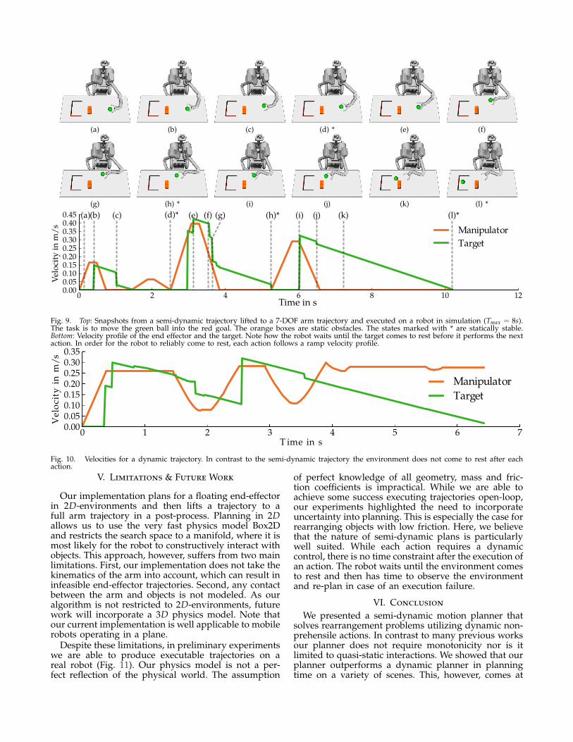
Fig. 10 shows the velocity profile for a trajectoryplanned with the dynamic planner on the same scene.Note how both the manipulator and the target objectkeep in motion for the whole trajectory. As a result thetotal duration of the trajectory is shorter than the semi-dynamic one. In fact, on average the solutions found bythe dynamic planner are shorter in execution time forscenes with dynamically behaving objects.

In Fig. 7 the average execution time is shown on

Scene 1 Scene 2 Scene 30

20

40

60

80

100

120

140

Avera

geexecu

tiontime(s)

Tmax = 0sTmax = 1sTmax = 8sTmax = 20sTmax = 60sDynamic

Fig. 7. Average path durations with standard deviation for threedifferent scenes in comparison (also see Fig. 8). Note that there wasonly a single path found for Tmax = 0s in Scene 3.

(a) Scene 1 (b) Scene 2 (c) Scene 3Type Scene 1 Scene 2 Scene 3Tmax = 0s 0.98± 0.02 0.25± 0.08 0.026± 0.024Tmax = 1s 0.98± 0.02 0.39± 0.09 0.10± 0.05Tmax = 8s 0.98± 0.02 0.98± 0.02 0.05± 0.04Tmax = 20s 0.98± 0.02 0.98± 0.02 0.06± 0.04Tmax = 60s 0.98± 0.02 0.98± 0.02 0.30± 0.08Dynamic 0.73± 0.08 0.90± 0.05 0.27± 0.08

Fig. 8. Top: Three scenes: the green object is the target object,movable objects are blue and static obstacles are red or orange. Boxeshave high friction and balls are modeled as low friction discs. Thegreen circle marks the goal region. Bottom: Table showing the 95%Wilson confidence intervals[26] of the success rates for the differentplanners on the depicted scenes.

three different scenes for each choice of Tmax and thedynamic planner. In an environment with only highfriction objects (Fig. 7, Fig. 8, left) the path duration issimilar for all planners.

The second environment (Fig. 7, Fig. 8, middle) con-tains two low friction objects, depicted as balls. Inthis environment the average path duration is higherfor each Tmax than for the dynamic planner. The pathduration increases with Tmax. Note, however, that thesuccess rate on this scene is significantly lower forTmax = 0s, 1s than for larger Tmax (Fig. 8).

The last scene (Fig. 7, Fig. 8, right) proves to be dif-ficult for all planners. It contains a static wall blockingdirect access to the goal. Furthermore, the goal regionlies in open space, where no obstacle prevents the ballfrom overshooting the goal region. The semi-dynamicplanner with Tmax = 0s, 1s, 8s, 20s found only very fewsolutions. If a solution was found the path duration ison average shorter than for greater Tmax as it involvesless waiting time. For Tmax = 60s more solutions arefound, but the path duration on average is the longest.The dynamic planner achieved a similar success rate onthis environment, but it found paths with the shortestexecution times on average.

We run preliminary experiments on a real robot(Fig. 11), which are discussed in the next section.

(a) (b) (c) (d) * (e) (f)

(g) (h) * (i) (j) (k) (l) *

0 2 4 6 8 10 120.000.050.100.150.200.250.300.350.400.45 (l)*

Manipulator

Target

(c) (d)*(a)(b) (e) (f) (g) (h)* (i) (j) (k)

Time in s

Vel

oci

ty i

n m

/s

Fig. 9. Top: Snapshots from a semi-dynamic trajectory lifted to a 7-DOF arm trajectory and executed on a robot in simulation (Tmax = 8s).The task is to move the green ball into the red goal. The orange boxes are static obstacles. The states marked with * are statically stable.Bottom: Velocity profile of the end effector and the target. Note how the robot waits until the target comes to rest before it performs the nextaction. In order for the robot to reliably come to rest, each action follows a ramp velocity profile.

Fig. 10. Velocities for a dynamic trajectory. In contrast to the semi-dynamic trajectory the environment does not come to rest after eachaction.

V. Limitations & Future Work

Our implementation plans for a floating end-effectorin 2D-environments and then lifts a trajectory to afull arm trajectory in a post-process. Planning in 2Dallows us to use the very fast physics model Box2Dand restricts the search space to a manifold, where it ismost likely for the robot to constructively interact withobjects. This approach, however, suffers from two mainlimitations. First, our implementation does not take thekinematics of the arm into account, which can result ininfeasible end-effector trajectories. Second, any contactbetween the arm and objects is not modeled. As ouralgorithm is not restricted to 2D-environments, futurework will incorporate a 3D physics model. Note thatour current implementation is well applicable to mobilerobots operating in a plane.

Despite these limitations, in preliminary experimentswe are able to produce executable trajectories on areal robot (Fig. 11). Our physics model is not a per-fect reflection of the physical world. The assumption

of perfect knowledge of all geometry, mass and fric-tion coefficients is impractical. While we are able toachieve some success executing trajectories open-loop,our experiments highlighted the need to incorporateuncertainty into planning. This is especially the case forrearranging objects with low friction. Here, we believethat the nature of semi-dynamic plans is particularlywell suited. While each action requires a dynamiccontrol, there is no time constraint after the execution ofan action. The robot waits until the environment comesto rest and then has time to observe the environmentand re-plan in case of an execution failure.

VI. Conclusion

We presented a semi-dynamic motion planner thatsolves rearrangement problems utilizing dynamic non-prehensile actions. In contrast to many previous worksour planner does not require monotonicity nor is itlimited to quasi-static interactions. We showed that ourplanner outperforms a dynamic planner in planningtime on a variety of scenes. This, however, comes at

(a) (b) (c) (d)

(e) * (f) (g) * (h) *

0 1 2 3 4 5 6 7T ime in s

0.00

0.05

0.10

0.15

0.20

0.25

Ve

loci

tyin

m/

s

(a) (b) (c) (d) (e)* (f) (g)* (h)*

Fig. 11. Top: Snapshots from a semi-dynamic trajectory lifted to a 7-DOF arm trajectory and executed on the robot HERB (Tmax = 8s).The task is to move the white box to the left. Bottom: Velocity profile for the trajectory as planned. Note how multiple objects are pushedsimultaneously. Also the target object, the cup and one of the poptart boxes are moved multiple times. The statically stable states are markedwith *.

the cost of an increased execution time in case of thepresence of low friction objects. Hence, we highlighteda fundamental trade-off between decreased planningtime and increased execution time.

VII. Acknowledgments

The research leading to these results has receivedfunding from the European Union Seventh FrameworkProgramme under grant agreement no. 270273 (Xperi-ence), the International Center for Advanced Commu-nication Technologies (InterACT), the IGEL programfrom the College for Gifted Students of the Departmentof Informatics at Karlsruhe Institute of Technology andfrom the Toyota Motor Corporation and NASA NSTRFgrant #NNX13AL61H.

References

[1] Open Dynamics Engine. http://www.ode.org, 2000 (accessedAugust 2014.

[2] NVIDIA PhysX: Physics simulation for developers. http://www.nvidia.com, 2009.

[3] Box2d. http://box2d.org, 2010 (accessed August 2014).[4] Bullet physics library. http://bulletphysics.org, (accessed Au-

gust 2014).[5] J. Barry, K. Hsiao, L. P. Kaelbling, and T. Lozano-Pérez. Manip-

ulation with multiple action types. In ISER, 2012.[6] A. Cosgun, T. Hermans, V. Emeli, and M. Stilman. Push

planning for object placement on cluttered table surfaces. InIEEE/RSJ IROS, 2011.

[7] M. Dogar and S. Srinivasa. A framework for push-grasping inclutter. In RSS, 2011.

[8] M. Dogar and S. Srinivasa. A planning framework for non-prehensile manipulation under clutter and uncertainty. Au-tonomous Robots, 2012.

[9] M. R. Dogar, K. Hsiao, M. Ciocarlie, and S. S. Srinivasa. Physics-based grasp planning through clutter. In RSS, 2012.

[10] S. Goyal, A. Ruina, and J. Papadopoulos. Planar sliding withdry friction. part 1. limit surface and moment function. Wear,1991.

[11] M. Gupta and G. S. Sukhatme. Using manipulation primitivesfor brick sorting in clutter. In IEEE ICRA, 2012.

[12] R. D. Howe and M. R. Cutkosky. Practical force-motion modelsfor sliding manipulation. IJRR, 1996.

[13] S. M. LaValle. Rapidly-exploring random trees: A new tool forpath planning. 1998.

[14] S. M. LaValle and J. J. Kuffner. Randomized kinodynamicplanning. IJRR, 2001.

[15] K. Lynch and M. T. Mason. Stable pushing: Mechanics, control-lability, and planning. In WAFR, 1995.

[16] T. Mericli, M. Veloso, and H. L. Akin. Achievable push-manipulation for complex passive mobile objects using pastexperience. In AAMAS, 2013.

[17] D. Nieuwenhuisen, A. Stappen., and M. Overmars. An effectiveframework for path planning amidst movable obstacles. InWAFR, 2008.

[18] D. Schiebener, J. Morimoto, T. Asfour, and A. Ude. Integratingvisual perception and manipulation for autonomous learning ofobject representations. Adaptive Behavior, 2013.

[19] T. Siméon, J.-P. Laumond, J. Cortés, and A. Sahbani. Manipula-tion planning with probabilistic roadmaps. IJRR, 2004.

[20] S. Srinivasa, D. Ferguson, C. Helfrich, D. Berenson, A. Col-let, R. Diankov, G. Gallagher, G. Hollinger, J. Kuffner, andM. Weghe. HERB: A Home Exploring Robotic Butler. Au-tonomous Robots, 28(1):5–20, 2010.

[21] M. Stilman and J. Kuffner. Navigation among movable obstacles:Real-time reasoning in complex environments. In IEEE-RASHumanoids, 2004.

[22] M. Stilman, J. Schamburek, J. Kuffner, and T. Asfour. Manipu-lation planning among movable obstacles. In IEEE ICRA, 2007.

[23] I. Sucan, M. Moll, and L. Kavraki. The Open Motion PlanningLibrary. IEEE Robotics and Automation Magazine, 2012.

[24] H. van Hoof, O. Kroemer, and J. Peters. Probabilistic segmen-tation and targeted exploration of objects in cluttered environ-ments. IEEE Transactions on Robotics (TRo), 2014.

[25] G. Wilfong. Motion planning in the presence of movableobstacles. Annals of Mathematics and Artificial Intelligence, 1991.

[26] E. B. Wilson. Probable inference, the law of succession, andstatistical inference. Journal of the American Statistical Association,1927.

[27] S. Zickler and M. Velosa. Efficient physics-based planning:sampling search via non-deterministic tactics and skills. InAAMAS, 2009.

[28] C. Zito, R. Stolkin, M. Kopicki, and J. L. Wyatt. Two-level RRTplanning for robotic push manipulation. In IEEE/RSJ IROS,2012.