
KINETIC VISIBILITY - Computer Graphicsgraphics.stanford.edu/~olaf/d_orig.pdf · A probabilistic...
197
KINETIC VISIBILITY a dissertation submitted to the department of computer science and the committee on graduate studies of stanford university in partial fulfillment of the requirements for the degree of doctor of philosophy Olaf A. Hall-Holt August 2002
Transcript of KINETIC VISIBILITY - Computer Graphicsgraphics.stanford.edu/~olaf/d_orig.pdf · A probabilistic...

KINETIC VISIBILITY
a dissertation
submitted to the department of computer science
and the committee on graduate studies
of stanford university
in partial fulfillment of the requirements
for the degree of
doctor of philosophy
Olaf A. Hall-Holt
August 2002

c© Copyright by Olaf A. Hall-Holt 2002
All Rights Reserved
ii

I certify that I have read this dissertation and that, in my opinion,
it is fully adequate in scope and quality as a dissertation for the
degree of Doctor of Philosophy.
Leonidas Guibas(Principal Adviser)
I certify that I have read this dissertation and that, in my opinion,
it is fully adequate in scope and quality as a dissertation for the
degree of Doctor of Philosophy.
Marc Levoy
I certify that I have read this dissertation and that, in my opinion,
it is fully adequate in scope and quality as a dissertation for the
degree of Doctor of Philosophy.
Michel Pocchiola(ENS Paris, France)
Approved for the University Committee on Graduate Studies:
iii

iv
Preface
An essential component of 3D graphics applications is a method to determine visibility, namely to
determine which parts of a virtual scene should be drawn on the screen. The seminal paper of
Sutherland, Sproull, and Schumacker in 1974 predicted that one of the most promising avenues for
research on visibility would be to make use of frame-to-frame coherence, since in a typical computer
animation the visible portion of the scene does not change very much from one frame to the next.
In the time since this observation was made, however, practitioners and researchers alike have found
this type of coherence to be difficult to fully exploit.
In recent years two general tools for addressing this type of problem have been developed in
the computational geometry community: the visibility complex and Kinetic Data Structures. The
visibility complex is a combinatorial structure that captures visibility relationships among objects
in a scene and contextualizes the operation of many visibility algorithms. Kinetic Data Structures
provide a general framework for the development of efficient algorithms in a dynamic environment of
continuously moving objects. This dissertation explores various methods that result from applying
the Kinetic Data Structures framework to substructures of the visibility complex. The algorithms
described here are intended to bring theoretical tools for visibility algorithms closer to practical
settings where low memory requirements and scalability are primary concerns.
We propose a framework for computing visibility in the plane and in space that leverages temporal
coherence, through the use of orientable spatial data structures. We describe three algorithms and
associated data structures. The first algorithm is a generalization and adaptation of the classic
topological sweep algorithm to enable maintenance of visibility for a moving observer in a static two-
dimensional environment. The second algorithm maintains visibility for a point observer in a planar
environment of moving obstacles. A probabilistic analysis of the second algorithm demonstrates
that in a particular average case setting, the intrinsic complexity of maintaining visibility in a static
scene and in a moving scene is asymptotically identical, up to a poly-logarithmic factor in the scene
density. The third algorithm illustrates how tools for planar visibility maintenance can be used in
a scene of objects that all lie near to some fixed ground plane. An implementation of the third
algorithm indicates that this approach can be viable in practice for large scenes with millions of
objects.
v

vi

Acknowledgments
I am deeply grateful to many people who have made it possible and rewarding to live and work at
Stanford these last few years. First, I would like to acknowledge a wonderful rabbi from Nazareth,
who saved my life. He brings joy and meaning to all who love Him.
The Stanford graphics lab has been a great place for development as a researcher. My adviser,
Professor Leonidas Guibas, has pointed me toward ever higher levels of scholarship, both by example
and by amazingly insightful feedback. Professor Marc Levoy has inspired me with his practical
wisdom and daring projects. Many of the students in the lab have helped me or have simply been
very enjoyable to see and talk with, and I would like to specifically mention just a few of them.
My closest collaborator and friend, Szymon Rusinkiewicz, worked and played and argued with me
through several years that I will never forget— God bless him! Joao Comba and Julien Basch
taught me the ropes as a beginning Ph.D. student, generously sharing their time and experience.
Menelaos Karavelas and I talked through many research ideas together in our shared office. When I
got stuck or needed to brainstorm on a new topic, Sean Anderson listened and often knew the next
step. Daniel Russell and Natasha Gelfand have consistently provided useful feedback and practical
help, with a smile! Li-Wei He and Lucas Pereira collaborated with me on some early and formative
projects. Alon Efrat helped me to hope for better results than I thought I could get. I’d like to
especially thank Afra Zomorodian, who was willing to participate in my defense, and Li Zhang, who
encouraged me in numerous ways through the years.
Other researchers outside of Stanford have also helped me a great deal during this period, and
I’d like especially to thank Professor Pankaj Agarwal, who discussed visibility problems with me
during a sabbatical at Stanford, and Professor Michel Pocchiola, whose work has been the source of
many of the ideas in this dissertation.
Through both the highs and lows of graduate student life, I have been supported by a vibrant
faith community, including many in the Stanford InterVarsity Graduate Christian Fellowship. I
will not attempt to mention all those deserving thanks, but I want to particularly acknowledge
Rishi Goyal, Jenny George, Rick Hernandez, Jen Amyx, Kim Norman, Mark Wistey, Aaron Stump,
Othar Hansson, the Clendenins and Schoutens, and especially our dear fellow married couples: the
Cutlers, Esselinks, Osborns, Primuths, Millers, Jacksons, Lewises, and Smiths. Another community
vii

that has supported me lives in Minnesota, including my wonderful Mom and Dad whose love has
been unwavering over decades (thank you!!!) and special thanks to my dear cousin Louise Lystig
Fritchie who patiently read and commented on all the chapters.
Finally, to my beloved wife Christy, whose beauty, courage, and faithfulness help define the best
parts of this shared adventure, I dedicate this manuscript.
viii

Contents
Preface v
Acknowledgments vii
1 Introduction 1
1.1 Research Problem and Significance . . . . . . . . . . . . . . . . . . . . . . . . . . . . 2
1.2 Brief Overview of the Literature . . . . . . . . . . . . . . . . . . . . . . . . . . . . . 2
1.3 Contribution of Research . . . . . . . . . . . . . . . . . . . . . . . . . . . . . . . . . 3
1.4 Research Hypothesis . . . . . . . . . . . . . . . . . . . . . . . . . . . . . . . . . . . . 4
2 Literature Review 5
2.1 The Visibility Complex . . . . . . . . . . . . . . . . . . . . . . . . . . . . . . . . . . 5
2.2 Kinetic Data Structures . . . . . . . . . . . . . . . . . . . . . . . . . . . . . . . . . . 7
2.3 Brief History of Temporally Coherent Point Visibility Algorithms . . . . . . . . . . . 8
2.4 Conclusion . . . . . . . . . . . . . . . . . . . . . . . . . . . . . . . . . . . . . . . . . 12
3 Static Objects: The Visible Zone 13
3.1 Problem Statement . . . . . . . . . . . . . . . . . . . . . . . . . . . . . . . . . . . . . 14
3.2 The Radial Subdivision . . . . . . . . . . . . . . . . . . . . . . . . . . . . . . . . . . 14
3.2.1 Definition of the Radial Subdivision . . . . . . . . . . . . . . . . . . . . . . . 15
3.2.2 Kinetic Maintenance of the Radial Subdivision . . . . . . . . . . . . . . . . . 16
3.2.3 Discussion . . . . . . . . . . . . . . . . . . . . . . . . . . . . . . . . . . . . . . 17
3.3 The Visible Zone: Definition and Kinetic Algorithm . . . . . . . . . . . . . . . . . . 18
3.3.1 Definition of a Visible Zone . . . . . . . . . . . . . . . . . . . . . . . . . . . . 18
3.3.2 Kinetic Maintenance of the Visible Zone . . . . . . . . . . . . . . . . . . . . . 20
3.4 The Visible Zone: Query Structure . . . . . . . . . . . . . . . . . . . . . . . . . . . . 24
3.5 The Visible Zone: Combinatorial Properties . . . . . . . . . . . . . . . . . . . . . . . 25
3.5.1 Redefinition of the Visible Zone . . . . . . . . . . . . . . . . . . . . . . . . . . 26
3.5.2 Correctness of the Event-Finding Procedure . . . . . . . . . . . . . . . . . . . 28
ix
3.5.3 Sequences of Elementary Steps . . . . . . . . . . . . . . . . . . . . . . . . . . 30
3.5.4 Effect of Observer Motion . . . . . . . . . . . . . . . . . . . . . . . . . . . . . 32
3.6 The Visible Zone: Worst Case Complexity . . . . . . . . . . . . . . . . . . . . . . . . 33
3.7 Extension of the Visible Zone to Moving Objects . . . . . . . . . . . . . . . . . . . . 34
4 Moving Objects: The Corner Arc Algorithm 37
4.1 Problem Statement and Kinetic Approach . . . . . . . . . . . . . . . . . . . . . . . . 38
4.2 Spatial Data Structure . . . . . . . . . . . . . . . . . . . . . . . . . . . . . . . . . . . 39
4.2.1 Definition of Boundary Segments . . . . . . . . . . . . . . . . . . . . . . . . . 39
4.2.2 Definition of Corner Arcs . . . . . . . . . . . . . . . . . . . . . . . . . . . . . 40
4.2.3 Definition of a Pseudo-triangulation . . . . . . . . . . . . . . . . . . . . . . . 42
4.3 Initialization of the Corner Arc Algorithm . . . . . . . . . . . . . . . . . . . . . . . . 44
4.3.1 Initialization of a Pseudo-triangulation . . . . . . . . . . . . . . . . . . . . . . 45
4.3.2 Initialization of Boundary Segments . . . . . . . . . . . . . . . . . . . . . . . 45
4.3.3 Initialization of Corner Arcs . . . . . . . . . . . . . . . . . . . . . . . . . . . . 45
4.3.4 Embedding Individual Corner Arcs . . . . . . . . . . . . . . . . . . . . . . . . 46
4.3.5 Embedding Shared Corner Arcs . . . . . . . . . . . . . . . . . . . . . . . . . . 47
4.4 Events and Event Handling . . . . . . . . . . . . . . . . . . . . . . . . . . . . . . . . 48
4.4.1 Events for Maintaining Boundary Segments . . . . . . . . . . . . . . . . . . . 49
4.4.2 Events for Maintaining Corner Arcs . . . . . . . . . . . . . . . . . . . . . . . 50
4.4.3 Events for Maintaining a Pseudo-triangulation . . . . . . . . . . . . . . . . . 53
4.4.4 Other Event Types . . . . . . . . . . . . . . . . . . . . . . . . . . . . . . . . . 56
4.5 Extensions . . . . . . . . . . . . . . . . . . . . . . . . . . . . . . . . . . . . . . . . . . 56
4.5.1 Changing object shape . . . . . . . . . . . . . . . . . . . . . . . . . . . . . . . 57
4.5.2 Viewing frustum . . . . . . . . . . . . . . . . . . . . . . . . . . . . . . . . . . 57
4.5.3 Non-convex objects . . . . . . . . . . . . . . . . . . . . . . . . . . . . . . . . . 57
4.5.4 Overlapping objects . . . . . . . . . . . . . . . . . . . . . . . . . . . . . . . . 57
5 Probabilistic Analysis for the Corner Arc Algorithm 59
5.1 Setting . . . . . . . . . . . . . . . . . . . . . . . . . . . . . . . . . . . . . . . . . . . . 59
5.2 Scene Characteristics . . . . . . . . . . . . . . . . . . . . . . . . . . . . . . . . . . . . 61
5.3 Corner Arc Algorithm Complexity . . . . . . . . . . . . . . . . . . . . . . . . . . . . 64
5.3.1 Cost of Tangency Events . . . . . . . . . . . . . . . . . . . . . . . . . . . . . 65
5.3.2 Cost of Other Event Types . . . . . . . . . . . . . . . . . . . . . . . . . . . . 71
5.4 Conclusion . . . . . . . . . . . . . . . . . . . . . . . . . . . . . . . . . . . . . . . . . 73
x

6 2D Implementation Results 75
6.1 An Average Case Setting . . . . . . . . . . . . . . . . . . . . . . . . . . . . . . . . . 75
6.2 Visibility-Related Characteristics . . . . . . . . . . . . . . . . . . . . . . . . . . . . . 76
6.3 Algorithm Comparison . . . . . . . . . . . . . . . . . . . . . . . . . . . . . . . . . . . 79
6.3.1 Radial Subdivision Algorithm . . . . . . . . . . . . . . . . . . . . . . . . . . . 79
6.3.2 Uniform Grid Algorithm . . . . . . . . . . . . . . . . . . . . . . . . . . . . . . 80
6.3.3 Visible Zone Algorithm . . . . . . . . . . . . . . . . . . . . . . . . . . . . . . 80
6.3.4 Corner Arc Algorithm . . . . . . . . . . . . . . . . . . . . . . . . . . . . . . . 80
6.4 Total Performance . . . . . . . . . . . . . . . . . . . . . . . . . . . . . . . . . . . . . 89
7 Extension to 3D 93
7.1 Background . . . . . . . . . . . . . . . . . . . . . . . . . . . . . . . . . . . . . . . . . 94
7.2 Problem Statement . . . . . . . . . . . . . . . . . . . . . . . . . . . . . . . . . . . . . 95
7.3 3D Radial Sweep Algorithm . . . . . . . . . . . . . . . . . . . . . . . . . . . . . . . . 95
7.4 Maintaining an Extended Ray . . . . . . . . . . . . . . . . . . . . . . . . . . . . . . . 97
7.4.1 Initializing the Sweep Plane . . . . . . . . . . . . . . . . . . . . . . . . . . . . 97
7.4.2 Locating 3D Objects with an Extended Ray . . . . . . . . . . . . . . . . . . . 99
7.4.3 Maintaining the Ground Query Segment . . . . . . . . . . . . . . . . . . . . . 99
7.5 Complex Occlusion and Transparency . . . . . . . . . . . . . . . . . . . . . . . . . . 100
7.6 Performance Comparison . . . . . . . . . . . . . . . . . . . . . . . . . . . . . . . . . 101
7.6.1 Accuracy of the Computed Visible Set . . . . . . . . . . . . . . . . . . . . . . 102
7.6.2 Computational Efficiency . . . . . . . . . . . . . . . . . . . . . . . . . . . . . 104
7.7 Extensions . . . . . . . . . . . . . . . . . . . . . . . . . . . . . . . . . . . . . . . . . . 105
7.8 Conclusion . . . . . . . . . . . . . . . . . . . . . . . . . . . . . . . . . . . . . . . . . 106
8 Conclusion 107
8.1 Summary of Results . . . . . . . . . . . . . . . . . . . . . . . . . . . . . . . . . . . . 107
8.2 Limitations . . . . . . . . . . . . . . . . . . . . . . . . . . . . . . . . . . . . . . . . . 108
8.3 Relation to Prior Research . . . . . . . . . . . . . . . . . . . . . . . . . . . . . . . . . 109
8.4 Future Work . . . . . . . . . . . . . . . . . . . . . . . . . . . . . . . . . . . . . . . . 109
A Zone Propogation Lemma 111
A.1 Towers and Spiralettes . . . . . . . . . . . . . . . . . . . . . . . . . . . . . . . . . . . 111
A.2 Elements of a Single Tower . . . . . . . . . . . . . . . . . . . . . . . . . . . . . . . . 111
A.3 Spiral Edges and Edge Types . . . . . . . . . . . . . . . . . . . . . . . . . . . . . . . 112
A.4 Paths . . . . . . . . . . . . . . . . . . . . . . . . . . . . . . . . . . . . . . . . . . . . 113
A.5 Shapes of Spiralettes and Edges . . . . . . . . . . . . . . . . . . . . . . . . . . . . . . 113
A.6 Vertex Types . . . . . . . . . . . . . . . . . . . . . . . . . . . . . . . . . . . . . . . . 114
xi

A.7 Types of Faces . . . . . . . . . . . . . . . . . . . . . . . . . . . . . . . . . . . . . . . 114
A.8 Tower Trees and the Face Order . . . . . . . . . . . . . . . . . . . . . . . . . . . . . 116
A.9 Spiral Edges . . . . . . . . . . . . . . . . . . . . . . . . . . . . . . . . . . . . . . . . . 116
A.10 Chords . . . . . . . . . . . . . . . . . . . . . . . . . . . . . . . . . . . . . . . . . . . . 117
A.11 Forward Paths . . . . . . . . . . . . . . . . . . . . . . . . . . . . . . . . . . . . . . . 119
A.12 Diagonal Paths . . . . . . . . . . . . . . . . . . . . . . . . . . . . . . . . . . . . . . . 120
A.13 Conservative Paths . . . . . . . . . . . . . . . . . . . . . . . . . . . . . . . . . . . . . 121
A.14 Branches . . . . . . . . . . . . . . . . . . . . . . . . . . . . . . . . . . . . . . . . . . . 121
A.15 Branch Face Lemma . . . . . . . . . . . . . . . . . . . . . . . . . . . . . . . . . . . . 124
A.16 Zone Propagation . . . . . . . . . . . . . . . . . . . . . . . . . . . . . . . . . . . . . . 124
B Elementary Step Sequences 127
B.1 Zone Transformations . . . . . . . . . . . . . . . . . . . . . . . . . . . . . . . . . . . 127
B.1.1 Definition . . . . . . . . . . . . . . . . . . . . . . . . . . . . . . . . . . . . . . 128
B.1.2 Properties of Composite Steps . . . . . . . . . . . . . . . . . . . . . . . . . . 128
B.1.3 Equivalent Transformations . . . . . . . . . . . . . . . . . . . . . . . . . . . . 130
B.1.4 General Sequences . . . . . . . . . . . . . . . . . . . . . . . . . . . . . . . . . 134
B.1.5 Minimum Length Transformations . . . . . . . . . . . . . . . . . . . . . . . . 139
B.2 Motion and Zone Connectivity . . . . . . . . . . . . . . . . . . . . . . . . . . . . . . 142
B.2.1 Definition of Triple Events . . . . . . . . . . . . . . . . . . . . . . . . . . . . . 143
B.2.2 Triple Events and Elementary Transformations . . . . . . . . . . . . . . . . . 144
B.2.3 Triple Events and General Transformations . . . . . . . . . . . . . . . . . . . 146
B.2.4 Triple Events on Cut Edges . . . . . . . . . . . . . . . . . . . . . . . . . . . . 148
B.2.5 Restricted Vertices . . . . . . . . . . . . . . . . . . . . . . . . . . . . . . . . . 150
B.3 Zone Maintenance Algorithms . . . . . . . . . . . . . . . . . . . . . . . . . . . . . . . 151
B.3.1 Elementary Transformations . . . . . . . . . . . . . . . . . . . . . . . . . . . 151
B.3.2 General Transformations . . . . . . . . . . . . . . . . . . . . . . . . . . . . . . 155
B.4 Lower Envelope Zones . . . . . . . . . . . . . . . . . . . . . . . . . . . . . . . . . . . 156
B.4.1 Acyclicity in Anti-Chains . . . . . . . . . . . . . . . . . . . . . . . . . . . . . 156
B.4.2 Lower Envelope Maintenance . . . . . . . . . . . . . . . . . . . . . . . . . . . 157
B.5 Visible Zone Maintenance . . . . . . . . . . . . . . . . . . . . . . . . . . . . . . . . . 158
B.5.1 Visible Zone Cyclicity . . . . . . . . . . . . . . . . . . . . . . . . . . . . . . . 158
B.5.2 Observer Motion . . . . . . . . . . . . . . . . . . . . . . . . . . . . . . . . . . 159
B.5.3 General Motion . . . . . . . . . . . . . . . . . . . . . . . . . . . . . . . . . . . 159
B.6 Amortized Complexity . . . . . . . . . . . . . . . . . . . . . . . . . . . . . . . . . . . 160
B.6.1 Wind Angles . . . . . . . . . . . . . . . . . . . . . . . . . . . . . . . . . . . . 160
B.6.2 Representative Maximal Segments . . . . . . . . . . . . . . . . . . . . . . . . 163
B.6.3 Amortized Complexity Analysis . . . . . . . . . . . . . . . . . . . . . . . . . . 165
xii

C Glossary 167
Bibliography 173
xiii

List of Tables
4.1 Sequence of operations for initializing the kinetic data structure. N is the number
of objects, v is the number of boundary segments, and t is the maximum number of
objects along the boundary of pseudo-triangles that intersect any given ray from the
observer. . . . . . . . . . . . . . . . . . . . . . . . . . . . . . . . . . . . . . . . . . . . 44
4.2 The types of events used to maintain visibility with corner arcs. . . . . . . . . . . . . 49
xiv

List of Figures
3.1 The area in yellow (visibility polygon) indicates what the observer (red dot) can see
as the observer moves past the objects (blue rectangles). . . . . . . . . . . . . . . . 13
3.2 The radial subdivision consists of a set of segments tangent to scene objects and
aligned with the observer. . . . . . . . . . . . . . . . . . . . . . . . . . . . . . . . . 13
3.3 The visible zone, like the radial subdivision, consists of a set of segments tangent
to scene objects. Updates, however, are applied only as needed. As a result, fewer
combinatorial updates are required to maintain the visible zone than the radial sub-
division. . . . . . . . . . . . . . . . . . . . . . . . . . . . . . . . . . . . . . . . . . . 14
3.4 The combinatorial description of any given tangent segment includes the object and
the object’s side on which it is tangent, the forward and back objects, and the three
neighboring tangent segments (shown here in black). . . . . . . . . . . . . . . . . . . 15
3.5 An elementary step of type “right-right”. A mirror image of this configuration re-
sults in a “left-left” elementary step. Elementary steps are the essential updates for
maintaining radial subdivisions and visible zones. . . . . . . . . . . . . . . . . . . . 17
3.6 The three frames on the left show how a radial subdivision changes as the observer
moves from the lower left to the lower right of the scene. The three frames on the
right show a visible zone. . . . . . . . . . . . . . . . . . . . . . . . . . . . . . . . . . 19
3.7 As the observer moves, two neighboring tangent segments attached to the observer
become momentarily collinear, thus requiring an update to their combinatorial de-
scriptions. . . . . . . . . . . . . . . . . . . . . . . . . . . . . . . . . . . . . . . . . . 20
3.8 Locating the appropriate object for the next event associated with tangent segment
Tright involves searching among the objects connected to its forward object F . The
frames above show the initial radial subdivision (a), and the visible zone just before
the event (b). Some tangent segments have not been drawn, for clarity. . . . . . . . 21
3.9 A recursive cascade of elementary steps. . . . . . . . . . . . . . . . . . . . . . . . . . 23
3.10 A tangent segment slides from one vertex to another. Such sliding motions may also
occur as tangent segments attached to the observer change angle. . . . . . . . . . . . 24
xv

3.11 The first frame above is the last frame of Figure 3.6, where an observer has moved
from the lower left of the scene to the lower right while maintaining the visible zone.
The second frame shows the effect of an extended ray query. Tangent segments near
the ray are made to line up with the ray, while those farther away are unaffected. . 26
3.12 An abstract depiction of an elementary step, where the cut moves up or down over a
vertex of the visibility complex by substituting two new cut edges. . . . . . . . . . . 28
3.13 Cases for determining the next elementary step as the tangent segment Tright turns
counter-clockwise about T . . . . . . . . . . . . . . . . . . . . . . . . . . . . . . . . . 29
3.14 Segments defining the faces f and g next to the tangent segment Tright. . . . . . . . 29
3.15 Segments belonging to two faces f2 and g2 just below the vertex defining the next
elementary step. As usual, this vertex is a maximal segment, not a vertex of a polygon. 30
3.16 The scene above depicts a visible zone with the observer in the center. If the topmost
object is moved up a distance equal to a tenth of its height, no tangent segments will
be disturbed, but the resulting configuration no longer represents a visible zone: it is
no longer connected via elementary steps to the radial subdivision. . . . . . . . . . . 34
4.1 The boundary of the visibility polygon shown in (a) consists of an alternating sequence
of parts of objects boundaries and segments through free space. These segments,
shown in (b), are called boundary segments. . . . . . . . . . . . . . . . . . . . . . . . 40
4.2 An example of a tangency event, where a particular boundary segment moves from
one far object to another. . . . . . . . . . . . . . . . . . . . . . . . . . . . . . . . . . 40
4.3 A corner arc can be obtained from a boundary segment by imagining that the segment
is made of elastic and pulling the end of the segment along the far object, away from
the visibility polygon, until it becomes tangent to the far object. . . . . . . . . . . . 41
4.4 A shared corner arc arises when two boundary segments face each other along the
same far object (a). In this situation, individual corner arcs would cross (b), so instead
a single corner arc is defined for both boundary segments (c). . . . . . . . . . . . . . 42
4.5 The requirements for non-intersection of bitangents are formulated as though the
polygons were actually slightly rounded at the vertices. The rounding would have the
effect of causing the bitangents in (a) to cross, and hence is not allowed, whereas in
(b) the bitangents would merely move apart, and so both would be permitted in the
same pseudo-triangulation. . . . . . . . . . . . . . . . . . . . . . . . . . . . . . . . . 43
4.6 A pseudo-triangulation (a) can easily be modified to include a particular corner arc:
flip each of the bitangents that intersect the interior of the corner arc region, in the
order determined by moving from the tangent point of the boundary segment to the
far object (b), and then along the far object to the end of the corner arc (c). . . . . 46
xvi

4.7 The construction of a shared corner arc proceeds as though individual arcs are being
computed. In (a), the corner arc for the boundary segment on the right is computed.
In (b), by the time ClearSeg reaches the corner arc calculated in (a), the shared corner
arc is in place. Some bitangents have been omitted from this figure for clarity. . . . . 48
4.8 A peek event turns one boundary segment into two boundary segments (a), and an
unpeek event reverses this operation (b). . . . . . . . . . . . . . . . . . . . . . . . . 50
4.9 A shaft event also turns one boundary segment into two boundary segments (a), and
an unpeek event reverses this operation (b). . . . . . . . . . . . . . . . . . . . . . . 50
4.10 A peek event requires construction of a new corner arc for the near boundary segment. 51
4.11 An unpeek event may require updating three boundary segments: the near and far
boundary segments, as well as the opposite boundary segment of the near boundary
segment (if there is a shared corner arc). . . . . . . . . . . . . . . . . . . . . . . . . . 52
4.12 A shaft event may require the construction of two shared corner arcs. . . . . . . . . 52
4.13 Four boundary segments are involved in this particular unshaft event. Because either
of the boundary segments on the opposite ends of the shared corner arcs could have
bitangents that block the formation of the new shared corner arc, the embedding
operation is applied to both of them. . . . . . . . . . . . . . . . . . . . . . . . . . . 53
4.14 A pseudo-triangle event involves moving one end of a bitangent to the endpoint of
another bitangent whenever two bitangents become collinear. For example, going
from left to right, the upper endpoint of a moves to the upper endpoint of b. . . . . 54
4.15 In this figure, the observer is stationary, and one object is moving. When any object
joins or leaves a corner arc, the pseudo-triangle events will preserve the corner arc
correctly. Some bitangents have not been drawn for clarity. . . . . . . . . . . . . . . 54
4.16 In this figure, the observer is stationary, and one object is moving. The third frame
shows what happens if the reflex update chooses the wrong invariant edge: the corner
arc is destroyed. Some bitangents and the boundary segments for the moving object
have not been drawn. . . . . . . . . . . . . . . . . . . . . . . . . . . . . . . . . . . . 55
5.1 A random scene with s = 3. . . . . . . . . . . . . . . . . . . . . . . . . . . . . . . . . 60
5.2 A random scene with s = 6. . . . . . . . . . . . . . . . . . . . . . . . . . . . . . . . . 60
5.3 A red point at distance r from a circle of the scene, and three zones between the point
and the circle. . . . . . . . . . . . . . . . . . . . . . . . . . . . . . . . . . . . . . . . . 62
6.1 The expected number of visible objects v compared with the actual number of visible
objects for a series of experiments. The averages and standard deviations are shown
in red, and the line of slope 1 is shown in green. . . . . . . . . . . . . . . . . . . . . . 77
xvii

6.2 The number of changes in visibility per second divided by s3 is shown in red, and
appears to be roughly constant. The expected constant of proportionality is shown
as a green line. . . . . . . . . . . . . . . . . . . . . . . . . . . . . . . . . . . . . . . . 77
6.3 The average number of two-object collisions per object per second (red) remains
steady as the number of objects increases, and the number of collisions with the
boundary (green) decreases (at v = 1000). . . . . . . . . . . . . . . . . . . . . . . . . 78
6.4 The average number of two-object collisions per object per second (red) decreases as
the distance between objects (expressed using v) increases. At the same time, the
number of collisions events along the boundary (green) remains steady. . . . . . . . . 79
6.5 The average edge length immediately after initialization of the pseudo-triangulation,
as a multiple of s. . . . . . . . . . . . . . . . . . . . . . . . . . . . . . . . . . . . . . . 81
6.6 The average length of edges in the scene increases slightly during the first few seconds,
but then remains steady thereafter. . . . . . . . . . . . . . . . . . . . . . . . . . . . . 81
6.7 The average number of pseudo-triangle events (red) and sliding events (green) per
object per second remains steady as the number of objects increases. . . . . . . . . . 82
6.8 For a fixed number of objects (N = 10, 000) the average number of pseudo-triangle
events per object per second (red) remains steady as the distance between objects
(expressed using v) increases. At the same time, the number of sliding events (green)
decreases slowly, as the influence of the reflective scene boundary declines. . . . . . . 82
6.9 The number of tangency events per second as a function of distance from the observer
(at v = 1000), compared to the expected average at those distances. . . . . . . . . . 83
6.10 The average age (red) of the arc edges at various distances from the observer, as
compared to a lower bound (green) on the expected time between the creation and
destruction of an arc edge (at v = 1000). . . . . . . . . . . . . . . . . . . . . . . . . . 84
6.11 A comparison of two ratios of edges to arc edges: 1) the population ratio among all
edges at a given distance from the observer (in red), 2) the ratio as discovered among
edges that are flipped during tangency events, at similar distances (in green). . . . . 84
6.12 The actual average number of flips per tangency event (red), and the expected upper
bounds on this quantity (green and blue), for various distances from the observer.
The frequency of tangency events grows small at large distances from the observer,
so the available data becomes more sparse. . . . . . . . . . . . . . . . . . . . . . . . 85
6.13 The number of flips per tangency event, as a function of the number of visible objects,
for a moving scene. . . . . . . . . . . . . . . . . . . . . . . . . . . . . . . . . . . . . . 85
6.14 The average number edges along triangles encountered during flips, as a function of
distance from the observer (at v = 1000). . . . . . . . . . . . . . . . . . . . . . . . . 86
6.15 The average number of edges along pseudo-triangles next to flipped edges. . . . . . . 86
xviii
6.16 The average number of pseudo-triangle (red) and sliding (green) events per object, at
various radii from the observer, when visibility is maintained. . . . . . . . . . . . . . 87
6.17 The average number of additional pseudo-triangle events, beyond the events expected
when visibility is not computed, per second as a multiple of s3 log s. . . . . . . . . . 88
6.18 The average number of CPU clock cycles required to handle each change in visibility
on an R10000 CPU. . . . . . . . . . . . . . . . . . . . . . . . . . . . . . . . . . . . . 88
6.19 The average number of tangency events (red) in the static case divided by s3, and the
expected constant of proportionality (green). . . . . . . . . . . . . . . . . . . . . . . 89
6.20 The average number of flips per tangency event in the static case appears to be about
2.5, even for very large scenes. . . . . . . . . . . . . . . . . . . . . . . . . . . . . . . . 89
6.21 The average size of pseudo-triangles encountered during flips. This graph matches
that for moving objects quite closely. . . . . . . . . . . . . . . . . . . . . . . . . . . . 90
6.22 The average number of CPU clock cycles required to handle each change in visibility
for a static scene on an R10000 CPU. . . . . . . . . . . . . . . . . . . . . . . . . . . 90
7.1 The intersection of the scene with the sweep plane shows the ground line, the sky
line, the observer, and several objects. . . . . . . . . . . . . . . . . . . . . . . . . . . 98
7.2 A forest scene. . . . . . . . . . . . . . . . . . . . . . . . . . . . . . . . . . . . . . . . 102
7.3 The underdraw of each of the four implemented variants, at various levels of trans-
parency. . . . . . . . . . . . . . . . . . . . . . . . . . . . . . . . . . . . . . . . . . . . 103
7.4 The overdraw of each of the four implemented variants, at various levels of transparency.103
7.5 The combination of overdraw and underdraw. . . . . . . . . . . . . . . . . . . . . . . 104
7.6 Timing data for each of the four algorithms tested. . . . . . . . . . . . . . . . . . . . 104
7.7 The time required by the most accurate variant compared to the rendering time. . . 105
B.1 a triple event . . . . . . . . . . . . . . . . . . . . . . . . . . . . . . . . . . . . . . . . 143
B.2 As the observer moves, two neighboring tangent segments attached to the observer
become momentarily collinear, thus requiring an update to their combinatorial de-
scriptions. . . . . . . . . . . . . . . . . . . . . . . . . . . . . . . . . . . . . . . . . . . 158
xix

xx

Chapter 1
Introduction
An artist painting a realistic picture often begins with elements of the background and proceeds to
overlay the foreground, so that objects nearer the observer occlude those further away. Computer
programs that render virtual scenes must also distinguish between those objects that are directly
visible to an observer, and those that cannot be seen due to occlusion. Automatic determination of
visible objects is an essential component of most graphics applications and is also used in fields as
diverse as robotics, product design, and urban planning.
For more than thirty years, researchers in the area of visibility algorithms have recognized the
importance of leveraging specific scene characteristics in designing computationally-efficient meth-
ods. Specifically, the degree to which a scene exhibits coherence in the clustering of objects and the
motion of the observer, among other such coherence attributes, may have a greater impact on the
running time of a visibility calculation than the total number objects in the scene. The difficulty of
characterizing these various types of coherence has led to a wide range of practical and theoretical
approaches.
The similarity between the set of objects visible in successive frames of an animation would seem
particularly useful when visibility is calculated many times for a moving observer. Although the set
of visible objects can change quickly – as when the observer sees around the corner of a building in an
urban setting – for many frames the visible set may change hardly at all, particularly if the motion
is slow. Such coherence may also exist if the objects of the scene are moving. The human visual
system appears to take advantage of temporal coherence in absorbing visual information. Research in
visibility algorithms has sought to use temporal coherence since the early days of computer-generated
pictures.
However, leveraging temporal coherence, particularly when scene objects are moving, remains
largely an unsolved problem. In typical graphics applications today, the set of visible objects is either
pre-calculated for static scenes, or recomputed nearly from scratch at every frame. As a result, few
algorithms utilize the prior or future positions of the observer, particularly when the objects of the
1
2 CHAPTER 1. INTRODUCTION
scene are moving. Although the potential value of temporal coherence for visibility calculations is
well-recognized, few methods are known for leveraging it effectively.
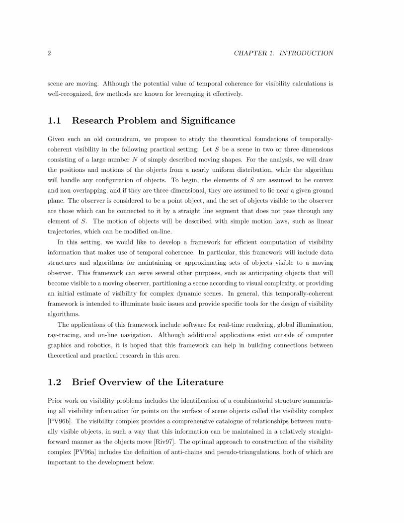
1.1 Research Problem and Significance
Given such an old conundrum, we propose to study the theoretical foundations of temporally-
coherent visibility in the following practical setting: Let S be a scene in two or three dimensions
consisting of a large number N of simply described moving shapes. For the analysis, we will draw
the positions and motions of the objects from a nearly uniform distribution, while the algorithm
will handle any configuration of objects. To begin, the elements of S are assumed to be convex
and non-overlapping, and if they are three-dimensional, they are assumed to lie near a given ground
plane. The observer is considered to be a point object, and the set of objects visible to the observer
are those which can be connected to it by a straight line segment that does not pass through any
element of S. The motion of objects will be described with simple motion laws, such as linear
trajectories, which can be modified on-line.
In this setting, we would like to develop a framework for efficient computation of visibility
information that makes use of temporal coherence. In particular, this framework will include data
structures and algorithms for maintaining or approximating sets of objects visible to a moving
observer. This framework can serve several other purposes, such as anticipating objects that will
become visible to a moving observer, partitioning a scene according to visual complexity, or providing
an initial estimate of visibility for complex dynamic scenes. In general, this temporally-coherent
framework is intended to illuminate basic issues and provide specific tools for the design of visibility
algorithms.
The applications of this framework include software for real-time rendering, global illumination,
ray-tracing, and on-line navigation. Although additional applications exist outside of computer
graphics and robotics, it is hoped that this framework can help in building connections between
theoretical and practical research in this area.
1.2 Brief Overview of the Literature
Prior work on visibility problems includes the identification of a combinatorial structure summariz-
ing all visibility information for points on the surface of scene objects called the visibility complex
[PV96b]. The visibility complex provides a comprehensive catalogue of relationships between mutu-
ally visible objects, in such a way that this information can be maintained in a relatively straight-
forward manner as the objects move [Riv97]. The optimal approach to construction of the visibility
complex [PV96a] includes the definition of anti-chains and pseudo-triangulations, both of which are
important to the development below.

1.3. CONTRIBUTION OF RESEARCH 3
A general framework for designing computationally-efficient methods in the context of moving
geometry has been developed under the name Kinetic Data Structures (KDS) [BGH99]. Examples
of KDSs include algorithms for efficient collision detection [ABG+00], maintenance of the Voronoi
diagram [Kar01], and kinetic BSP-trees [Com00]. The specific algorithms proposed below belong to
this general framework.
The history of theoretical research on visibility in the computational geometry community in-
cludes worst-case output sensitive methods for hidden surface removal [Dor94], general query struc-
tures for ray-shooting and other related ranges [AE99], and precise definitions for a few types of
object coherence found in typical scenes [dBKvdSV97]. Most of the work on temporally coherent
visibility has been undertaken in a worst-case setting, if precise bounds are available at all.
Practical approaches to visibility calculations developed by the computer graphics community
have often relied on the z-buffer, a hardware device that cannot by itself make use of temporal co-
herence. Instead, the z-buffer has often been used as the final step in algorithms that overestimate
the set of visible objects [ZMHI97] or as a means of sampling in determining objects visible from a
volume [DDTP00]. Other practical algorithms preprocess visibility for static scenes [SDDS00], de-
termine visibility in specialized settings such as urban environments [DMS01], or leverage additional
hardware resources.
1.3 Contribution of Research
The four principle contributions of this thesis are as follows:
1. The identification of new properties of the visibility complex relevant to point visibility main-
tenance. These properties include the existence and properties of a linear-sized substructure
of the visibility complex, called the visible zone, that can be used for temporally-coherent vis-
ibility calculations in the plane. The specific data structure proposed to implement the visible
zone synthesizes aspects of object-space and ray-space subdivision structures.
2. Data structures and algorithms addressing particular visibility problems. The visible zone
algorithm shows how a classic sweep algorithm can be transformed into a kinetic algorithm for
visibility maintenance. The corner arc algorithm provides an average-case near-optimal ap-
proach for maintaining the visible set among moving objects in the plane, based on maintaining
a novel invariant in a pseudo-triangulation.
3. A description of the practical results of implementing these planar algorithms, including a
verification of the probabilistic analysis and the associated constant factors.
4. A method for using planar, temporally-coherent visibility structures as the basis for three-
dimensional visibility algorithms. In collaboration with Szymon Rusikiewicz, I have built

4 CHAPTER 1. INTRODUCTION
and tested an interactive fly-through application for a large forest scene, and compared this
algorithm with the visibility algorithm of Downs et al. [DMS01].
This dissertation is organized as follows. Chapter 2 briefly reviews relevant literature. Chapter
3 describes a simple approach for maintaining visibility for a moving observer among static objects.
Chapter 4 describes an algorithm for maintaining visibility among moving objects. A probabilistic
analysis of the algorithm of chapter 4 is given in chapter 5. Chapter 6 presents implementation results
for the 2D visibility maintenance algorithms. Chapter 7 describes an extension of the algorithm of
chapter 3 to 3D, and compares it with another algorithm. Chapter 8 concludes.
1.4 Research Hypothesis
The general hypothesis to be investigated in this dissertation is whether kinetic methods based on
combinatorial structures arising from the visibility complex can efficiently leverage temporal coher-
ence in determining visibility for both static and moving scenes. The emphasis in this exploration
is on theoretical approaches; however, the goal is to remain close enough to practical application
domains so as to build toward practical algorithms. To this end, the principle algorithms developed
in the course of this investigation have all been implemented and tested on large datasets, and an
explicit comparison is given for the 3D case.

Chapter 2
Literature Review
Prior work devoted to problems of visibility has addressed many different aspects of visibility, from
robot navigation to the placement of guards in an art gallery for surveillance. A broad survey
[Dur99] indicates that much of this work for more than 30 years has focused on the problem of
computing what part of a virtual scene is visible to a virtual point observer. This is the specific
visibility problem studied in this thesis, with a focus on temporal coherence as a means to obtain
greater computational efficiency.
Over the years, some general tools have been developed to describe the underlying combinatorial
structure of visibility, as well as methods for designing geometric algorithms that leverage temporal
coherence. The first two sections in this chapter describe this foundational work on the visibility
complex and Kinetic Data Structures, respectively. The following section provides a tour of visibility
algorithms that leverage temporal coherence, beginning with work by Schumacker et al. in 1969. The
final section concludes with general observations.
2.1 The Visibility Complex
The visibility complex was introduced and refined by Pocchiola and Vegter [PV96b], [PV96a] and
later described in 3D by Durand et al. [DDP96], [DDP97b], [DDP97a]. At a high level, the visibility
complex is a way of describing all the visibility relationships among objects in a scene. If a point
on the boundary of one object can be connected to a point on the boundary of another object by
a straight line segment that does not intersect the interior of any other objects, then this segment
is represented within the visibility complex. In order to simplify the definitions and resulting com-
binatorial cases, the visibility complex is usually defined for the following smooth setting (in 2D or
3D).
Let S be a set of pairwise disjoint convex objects whose boundaries are ‘smooth’ in the following
sense: for each point on any object boundary, there exists a single well defined tangent (line or
5

6 CHAPTER 2. LITERATURE REVIEW
plane), and for each tangent (line or plane) to an object, there is exactly one tangent point. Also,
let us assume no tangent degeneracies, so that, for example, three objects are not allowed a common
tangent line in the plane, and four objects are not allowed a common tangent plane in space. The
free space is the space surrounding the objects of S, that is, the complement of the union of their
interiors. A maximal segment is a line segment of free space, such that it cannot be lengthened
along its supporting line without intersecting some object interior. (Technically, some of these
“segments” may be half-lines or lines.) In other words, maximal segments express visibility from
points on object boundaries to other objects in the scene (or infinity).
The visibility complex is the set of all maximal segments, grouped according to the objects
that they touch. Given a maximal segment m that is not tangent to any object, whose endpoints
lie on some objects A and B, m is grouped together with all other maximal segments that can be
obtained by moving the endpoints of m along the boundary of A and B without becoming tangent
to any object in the process. This group is called a face of the visibility complex in the 2D setting
or a 4-face in the 3D setting. Similarly, a maximal segment that is tangent at just one point to
some object is grouped together with those maximal segments that can be reached by moving the
endpoints and maintaining tangency to one object without becoming tangent to any other object
in the process. This group of maximal segments, each of which has exactly one tangent point, is
called an edge in 2D and a 3-face in 3D. In the plane, a maximal segment tangent to two objects
cannot be moved without destroying at least one tangency, so it is called a vertex. In space, maximal
segments with 2 tangencies make up 2-faces, those with 3 tangencies form edges, and those with
4 tangencies are the vertices. Thus the visibility complex is a cell complex defined over the set of
maximal segments.
The properties of the visibility complex are numerous, and depend on whether S is defined in
2D or 3D. In 3D, the visibility complex is potentially large and complicated, with Ω(n4) vertices in
the worst case and many 2-, 3-, and 4-faces that are not even simply connected. In the plane, the
visibility complex is simpler, having O(n2) vertices and simply connected faces. In particular, the
one-dimensional boundary of a face consists of a cyclic alternating sequence of edges and vertices.
The local connectivity of the 2D cell complex allows three faces to meet at an edge, and four edges
to meet in a vertex.
The visibility complex provides a unifying framework for describing visibility calculations, since
visibility along any set of rays can be understood as a subset of the visibility complex. However, most
visibility algorithms do not explicitly represent the entire visibility complex, due to its large size. In
chapter 3, we propose a linear size substructure of the visibility complex that can be represented and
maintained explicitly for the sake of visibility maintenance. A second linear size structure closely
related to the visibility complex, called a pseudo-triangulation [PV96c], has been found to be useful
in multiple contexts (e.g. [ABG+00]) and will also be described in chapter 4.

2.2. KINETIC DATA STRUCTURES 7
2.2 Kinetic Data Structures
In a physical setting that involves moving objects, motion is often considered to be continuous, in
the sense that the position of any point on any object is a continuous function of time. Even in
discrete simulations where positions are only available at discrete moments of time, the motion of an
object can often be considered continuous, by interpolation. In this setting of moving geometry, a
general framework for designing temporally coherent algorithms has been developed, called Kinetic
Data Structures (KDS) (e.g. [BGH99]).
Kinetic Data Structures are closely related to data structures used in event-based simulations.
Given a set of geometric objects, together with a description of their current motion, a KDS maintains
a geometric attribute of interest A. For example, A might be the closest pair of objects, or the set of
objects visible from a point. An event is a sudden change in geometric relationships, such as when
the attribute A changes suddenly, or when the geometric structure used to calculate A changes
suddenly, or when the motion of one or more of the objects changes suddenly. The overall approach
of a kinetic algorithm is to process these events in the order in which they occur, making updates
in the geometric data structure or the attribute A as necessary.
The design of a KDS can sometimes proceed directly from consideration of how A would be
calculated in a static setting. A geometric algorithm typically proceeds by computing a sequence of
geometric predicates on its input, and branching based on the results of these predicates. Given such
a static algorithm G, a KDS can be designed to mimic the behavior of G at some start time, and
then monitor the validity of the geometric predicates used by G as objects move. If these predicates
do not change, then the attribute A does not change either (at least not in a certain combinatorial
sense) since rerunning G would produce the same combinatorial result. On the other hand, if at
a certain moment one of these predicates changes, then this change is an event, and an update is
invoked to determine a new set of predicates that mimic a calculation of A.
The computational efficiency of a KDS cannot be measured in the same way that most geometric
algorithms are measured, since there is no particular termination to the calculation, and there may
not even be any termination to the input (for example, if the motion is specified on-line). Instead,
designers of KDSs have typically focused on the cost of individual event updates, as well as the
relationship between the number of events and the number of changes in A. The number of changes
in A is considered an unavoidable lower bound to the number of events, since the intent of a KDS
is to maintain A at all times, even if A is changing frequently.
The result of this approach is a kind of ‘pure’ focus on temporal coherence, since the cost of
a KDS is then entirely dependent on actual changes in geometric relationships, as opposed to the
frequency of an arbitrarily chosen set of time samples. From the point of view of designing geometric
algorithms that leverage temporal coherence, designing a KDS may be a good place to start, since it
will often illuminate critical geometric relationships that are important to time varying calculations.
However, KDSs are not always the best approach in practice, since an application may not need the
8 CHAPTER 2. LITERATURE REVIEW
attribute A at all times, but only at certain time samples.
2.3 Brief History of Temporally Coherent Point Visibility
Algorithms
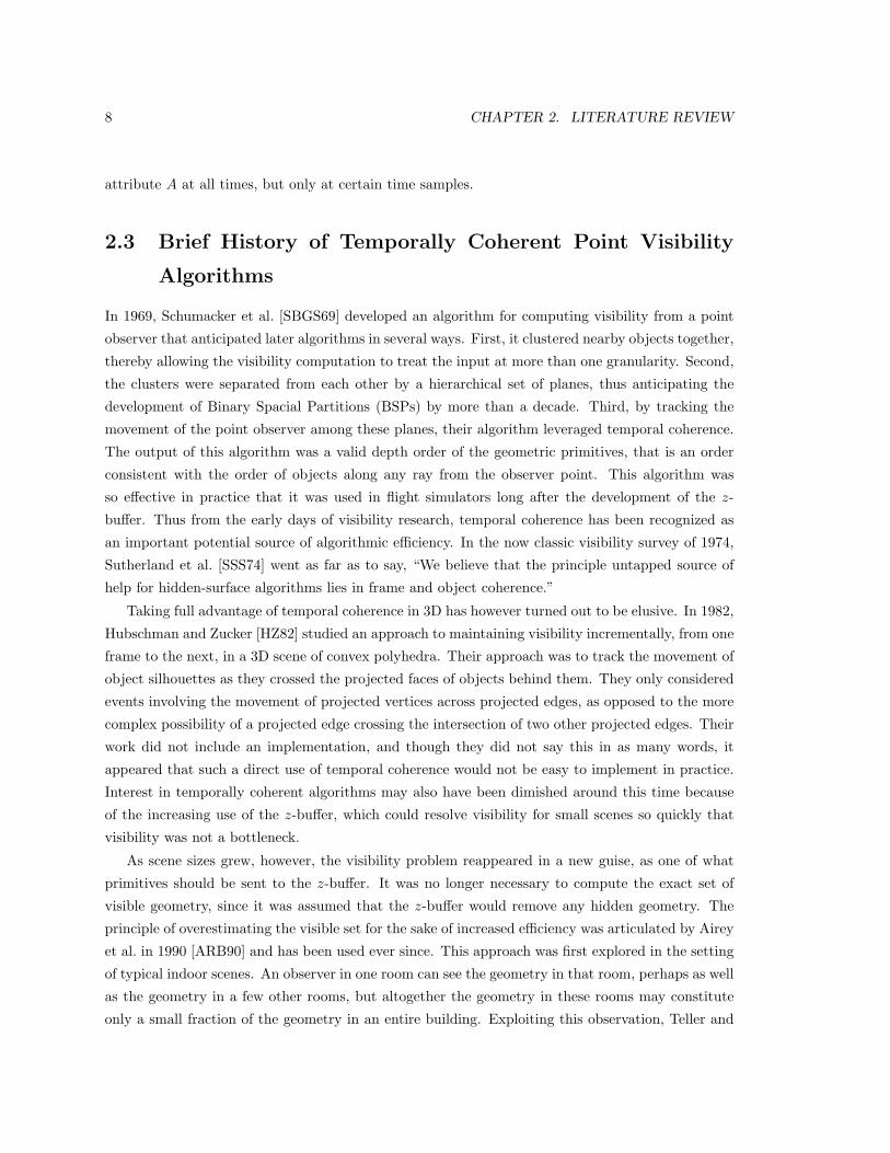
In 1969, Schumacker et al. [SBGS69] developed an algorithm for computing visibility from a point
observer that anticipated later algorithms in several ways. First, it clustered nearby objects together,
thereby allowing the visibility computation to treat the input at more than one granularity. Second,
the clusters were separated from each other by a hierarchical set of planes, thus anticipating the
development of Binary Spacial Partitions (BSPs) by more than a decade. Third, by tracking the
movement of the point observer among these planes, their algorithm leveraged temporal coherence.
The output of this algorithm was a valid depth order of the geometric primitives, that is an order
consistent with the order of objects along any ray from the observer point. This algorithm was
so effective in practice that it was used in flight simulators long after the development of the z-
buffer. Thus from the early days of visibility research, temporal coherence has been recognized as
an important potential source of algorithmic efficiency. In the now classic visibility survey of 1974,
Sutherland et al. [SSS74] went as far as to say, “We believe that the principle untapped source of
help for hidden-surface algorithms lies in frame and object coherence.”
Taking full advantage of temporal coherence in 3D has however turned out to be elusive. In 1982,
Hubschman and Zucker [HZ82] studied an approach to maintaining visibility incrementally, from one
frame to the next, in a 3D scene of convex polyhedra. Their approach was to track the movement of
object silhouettes as they crossed the projected faces of objects behind them. They only considered
events involving the movement of projected vertices across projected edges, as opposed to the more
complex possibility of a projected edge crossing the intersection of two other projected edges. Their
work did not include an implementation, and though they did not say this in as many words, it
appeared that such a direct use of temporal coherence would not be easy to implement in practice.
Interest in temporally coherent algorithms may also have been dimished around this time because
of the increasing use of the z-buffer, which could resolve visibility for small scenes so quickly that
visibility was not a bottleneck.
As scene sizes grew, however, the visibility problem reappeared in a new guise, as one of what
primitives should be sent to the z-buffer. It was no longer necessary to compute the exact set of
visible geometry, since it was assumed that the z-buffer would remove any hidden geometry. The
principle of overestimating the visible set for the sake of increased efficiency was articulated by Airey
et al. in 1990 [ARB90] and has been used ever since. This approach was first explored in the setting
of typical indoor scenes. An observer in one room can see the geometry in that room, perhaps as well
as the geometry in a few other rooms, but altogether the geometry in these rooms may constitute
only a small fraction of the geometry in an entire building. Exploiting this observation, Teller and

2.3. BRIEF HISTORY OF TEMPORALLY COHERENT POINT VISIBILITY ALGORITHMS 9
Sequin [TS91] (also [Tel92]) present methods for computing a subdivision of space conforming to a
set of walls, as well as the visibility relationships within this subdivision, that allow rapid estimates
of a superset of the visible geometry to be made at run time. This subdivision of space that the
observer moves through is once again the basis for a kind of temporal coherence: the estimated
visible set does not change significantly from one frame to the next while the observer remains in
the same room. The analogous problem in 2D of computing visibility in a polygon has been well
studied [CEG+94] and permits worst-case efficient solutions [AGTZ98].
Also in the early 1990s, research by Mulmuley [Mul91] and Bern et al. [BDEG94] examined
theoretical approaches to computing temporal coherence for a point observer moving along a known
linear trajectory in 3D. The algorithms they describe compute the locations along the trajectory
where the visible set changes. We call such a location where the visible set changes a coherence
boundary, namely the locus of points in space where a particular change in visibility occurs. In 3D,
these coherence boundaries are typically planes or quadratic ruled surfaces. Their work addressing
an observer moving along a fixed trajectory is perhaps the first to give non-trivial bounds on the
complexity of a visibility algorithm that depends on explicit calculation of coherence boundaries.
Unfortunately, these bounds depend not only on the number of intersected coherence boundaries,
but also on predicates operating on hidden geometry. The latter cost, which is dominant in the
worst case, appears difficult to avoid. That is, as we try to find those boundaries across which
the observer will see a change in visibility, it is necessary to search among geometry that is only
potentially, and not always, visible. Perhaps for this reason, as well as the mismatch between scenes
found in practice and worst-case examples, worst-case analysis of the maintenance of the visible set
has not yet yielded output-sensitive bounds for this type of problem. Other examples of visibility
algorithms in computational geometry, particularly for the case of no movement, are surveyed in
[Dor94].
Bringing together the themes of conservative over-estimation and temporal coherence based on
locating coherence boundaries, Coorg and Teller [CT96] [CT97] proposed a coarse subdivision of
the space around the observer in an outdoor scene. The coherence boundaries are chosen to arise
from considering a small number of occluders and large clusters of occludees. As with the work of
Hubschman and Zucker [HZ82], the coherence boundaries arise from the locations where a projected
vertex would appear to cross a projected edge, and both the vertex and the edge are assumed to
belong to convex polyhedra. As with the prior theoretical algorithms, the set of such coherence
boundaries is explicitly calculated. Several options are available for organizing the use of these
coherence boundaries.
In one approach [CT96], which is close to the kinetic approach, the motion of the observer is
assumed continuous, and incremental updates are triggered as the observer crosses the various coher-
ence boundaries. In the later approach [CT97] the continuity of observer motion is de-emphasized by
doing the updates in an order unrelated to the motion of the observer and calculating new coherence

10 CHAPTER 2. LITERATURE REVIEW
boundaries with reference to the new observer sample position. This latter approach preserves some
features of temporal coherence in using coherence boundaries to identify places in the scene where
new geometry may be revealed, yet is not as tied to the number of coherence boundaries crossed
per frame than the other algorithm. Another analogous trade-off between sampling and temporal
coherence will be presented in chapter 7.
With the development of the visibility complex, several authors have proposed methods based
directly or indirectly on the visibility complex for maintaining visibility. Riviere [Riv97] described
how to traverse the visibility complex to obtain the set of objects visible to an observer and the
changes that occur in the visibility complex due to object motion (see also [DORP96]). When made
explicit in an algorithm, these observations allow maintenance of the visible set under observer
and/or object motion. Due to the comprehensive representation of visibility information, individual
updates to the visibility complex as objects move are relatively simple and require only O(log n)
time each. The ease of updates largely translates into 3D as well, and [Dur99] catalogues the list of
relevant updates. On the other hand, the number of updates required to maintain this comprehensive
structure makes it less appealing for this application, since the number of events may far outstrip
the number of changes in the visible set. Also, no non-trivial bounds have been proposed for the
number of updates required in such an algorithm when objects other than the observer are moving.
Related work in the plane by Ghali and Stewart [GS96] focused on the relationship between the
observer and the coherence boundaries computable from the visibility complex. In particular, for a
static scene with a moving point observer in the plane, the coherence boundaries are lines and can be
dualized to points, while the observer point can be dualized to a line. In the dual plane, the crossing
of a coherence boundary becomes a line sweeping over a point. Rather than compare the moving
line with all the points in the dual, Ghali and Stewart maintained two convex hulls on each side of
the line, thus speeding up the identifications of crossed boundaries in practice. Characterizing the
complexity of this algorithm is challenging, since in the worst case there is no benefit to maintaining
the convex hull.
Further work on temporally coherent algorithms has sought to avoid storing the entire visibility
complex by relying on spatial subdivision structures. General purpose Kinetic Data Structures for
maintaining visibility with BSP trees in 3D were proposed by Comba [Com00] and Murali [Mur98].
They showed that, with the help of such a spatial subdivision, all necessary events for visibility
maintenance could be identified and appropriate updates performed. Other work on enabling motion
of objects in a BSP has been carried out for purposes of shadow calculations and radiosity (e.g.,
[Chr96]) demonstrating the versatility of BSP trees for addressing a variety of visibility problems in a
temporally coherent manner. Unfortunately, the constant factors in these algorithms are often high,
and there may also be problems arising from numerical imprecision. In addition, characterizing the
complexity of these algorithms continues to be a challenge, since the ‘typical’ behavior is so unlike
the worst case. In the plane, a temporally coherent subdivision similar to a vertical decomposition

2.3. BRIEF HISTORY OF TEMPORALLY COHERENT POINT VISIBILITY ALGORITHMS11
was proposed by Nechvile and Tobola [NT99b], but discussion of their work is deferred until chapter
3.
A different approach to eliminating geometry prior to sending it to the z-buffer is to seek to
eliminate large chunks of the scene hierarchically, as with the hierarchical z-buffer [GKM93] or
with hierarchical occlusion maps [ZMHI97] [Zha98]. The latter approaches select a set of candidate
occluders, build a query structure from them that can quickly reject occluded geometry, and traverse
the scene hierarchically. These techniques can make some use of temporal coherence in the selection
of occluders, since the visible geometry of one frame may provide a good hint as to the best occluders
to use for the next frame. However, there is no guarantee that this hint is a sufficient guess. If at
any frame this guess is inaccurate, that is the set of occluders obtained from the previous frame
is not representative, then the algorithm pays a high penalty. As a result, although this approach
has been discussed in the context of temporally coherent algorithms, in the actual implementation
Zhang [Zha98] dispensed with using temporal coherence, saying that the benefits are too small.
Another class of algorithms related to temporal coherence for reducing the amount of geometry
sent to the z-buffer consists of those that compute a conservative visible set for all possible observer
locations in a bounded region, rather than just from one point. If the observer moves within this
region for several frames, then the cost of computing visibility is amortized over these frames. This
calculation can be considerably more involved than computing visibility from a point, and a variety
of approximations and discretizations have been proposed. These methods include considering oc-
cluders one by one [COFHZ98], shrinking the size of occluders and doing a point-based calculation
[WWS00], restricting the computation to a regular spatial subdivision like an octree [SDDS00], and
conservative sampling methods [DDTP00]. In each case, the idea of motion has been converted into
a static spatial representation, and thus these techniques appear to apply best when the objects of
the scene are static. Another example of this approach to motion is given in [SG99], where objects
are allowed to move within a spatial subdivision, but the extent of their movement is modeled as
a region of space, which in turn is considered as though it were a static object. In this algorithm,
moving objects cannot contribute to occlusion of geometry behind them, and many moving objects
that are not visible may nevertheless be classified as potentially visible.
Among the methods for computing visibility from a region, Cohen-Or et al. [COFHZ98] are
notable in their analysis of complexity. Unlike most work in this field (see Durand [Dur99] for
another exception), Cohen-Or et al. provided an ‘average case’ type model of a scene that can be
used to estimate quantities like the expected number of objects visible from a small region based
on a small set of parameters. Their results were derived particularly for the from-region case, but
the average-case analysis of chapter 5 will begin with the setting of uniformly distributed objects
described there.
Yet another approach to visibility algorithms that seek to leverage temporal coherence is found
in research that assumes the presence of a uniform spatial subdivision, as in volume rendering or

12 CHAPTER 2. LITERATURE REVIEW
many instances of ray-tracing. In this setting, an apparently inefficient operation is to traverse a long
sequence of empty cells repeatedly. One approach to avoiding such operations is to construct cones
around rays [Ama84] to accelerate future queries in the same neighborhood. This approach was
found to be very expensive in practice. Another method stores the distance to the nearest geometry
from each empty cell, thus allowing leaps over sets of empty cells [CS94] [SK97]. These techniques
avoid computing coherence boundaries, and instead focus on leveraging temporal coherence within
some fast query structure.
2.4 Conclusion
The study of temporally coherent visibility algorithms for a point observer has evolved over more
than three decades from an emphasis on sorting the input geometry, to computing coherence bound-
aries instead of sorting, to avoiding coherence boundaries as well. In all this work, representative
asymptotic bounds on the time complexity of these algorithms have been difficult to obtain, and no
non-trivial bounds are known for the setting of no static objects. This thesis sets out to explore the
fundamental aspects of visibility and temporal coherence in a manner that permits the development
of asymptotic bounds for a moving observer in a static scene, as well as for an observer surrounded
by moving objects. The initial development will focus on kinetic algorithms, followed by methods
to reduce the dependence on explicit coherence boundaries.
Chapter 3
Static Objects: The Visible Zone
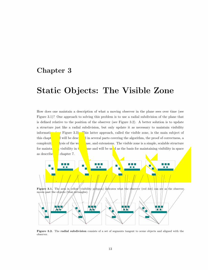
How does one maintain a description of what a moving observer in the plane sees over time (see
Figure 3.1)? One approach to solving this problem is to use a radial subdivision of the plane that
is defined relative to the position of the observer (see Figure 3.2). A better solution is to update
a structure just like a radial subdivision, but only update it as necessary to maintain visibility
information (see Figure 3.3). This latter approach, called the visible zone, is the main subject of
this chapter and will be described in several parts covering the algorithm, the proof of correctness, a
complexity analysis of the worst case, and extensions. The visible zone is a simple, scalable structure
for maintaining visibility in the plane and will be used as the basis for maintaining visibility in space
as described in chapter 7.
Figure 3.1. The area in yellow (visibility polygon) indicates what the observer (red dot) can see as the observermoves past the objects (blue rectangles).
Figure 3.2. The radial subdivision consists of a set of segments tangent to scene objects and aligned with theobserver.
13

14 CHAPTER 3. STATIC OBJECTS: THE VISIBLE ZONE
Figure 3.3. The visible zone, like the radial subdivision, consists of a set of segments tangent to scene objects.Updates, however, are applied only as needed. As a result, fewer combinatorial updates are required to maintain thevisible zone than the radial subdivision.
3.1 Problem Statement
The basic problem to be solved in this chapter is illustrated in Figure 3.1. A point observer (drawn
as a red dot) moves amid a set of rectangular obstacles, and we would like to continuously maintain a
description of the area visible to the observer (illustrated in yellow). This problem is the simplest non-
trivial visibility maintenance problem with multiple, unconnected occluders, and if efficient kinetic
solutions exist for more complex problems, there must be an efficient solution to this problem as
well.
Formally, let S be a set of N non-overlapping convex polygons in the plane in general position, so
that, for example, no three objects share a common tangent line. Let F be the free space surrounding
the polygons; namely, the complement of the union of the interiors of elements of S. Let p be a point
(the observer) that lies in F . The visibility polygon V (illustrated in yellow) is the set of points
in F such that a straight line segment from p to a point of V lies entirely within F . At any given
moment, the motion of the observer p is assumed to be described by a pseudo-algebraic function of
constant degree, such that p remains at all times in F . The function describing the movement of
p may be changed (say, in response to the movement of a mouse) as p moves. The problem is to
design an efficient on-line algorithm that maintains a list of the objects along the boundary of V at
all times as p moves. This list will be called the visible set, and may include an object more than
once if the object is visible in two distinct places along the visibility polygon.
The applications most in need of efficient visibility algorithms involve large numbers of scene
objects, often numbering in the millions. Thus from the outset we seek a solution that is efficient
with large scenes: one that uses only linear storage and which minimizes computation by focusing
changes in the data structure as much as possible on an area near to the observer.
3.2 The Radial Subdivision
One approach to this problem of maintaining visibility is to maintain a radial subdivision of the
plane about the observer [NT99b] [NT99a]. Although maintenance of the radial subdivision is not
scalable to large numbers of scene objects, this approach is integrally related to the better solution of
maintenance of the visible zone, and simpler to describe. This section defines the radial subdivision,

3.2. THE RADIAL SUBDIVISION 15
describes its initialization, and provides details on how it can be maintained as the observer moves.
The terminology and methods described in this section are essential to the solution described in the
rest of this chapter.
3.2.1 Definition of the Radial Subdivision
A radial sweep provides a direct method for computing the visibility polygon of an observer in a
static scene. This sweep can be used to build a (radial) trapezoidal subdivision of the plane that is
exactly analogous to the classic (vertical) trapezoidal subdivision. A radial subdivision consists of
the polygons of S together with a set of line segments, defined as follows.
Let l be a line through the point observer p that is also tangent to a polygon P of S. A tangent
segment of P is the connected portion of l incident to P that lies in free space. In other words, the
tangent segment is the part of l obtained by starting from the tangent point and extending toward
and away from the observer just enough to reach other objects (if any). Each of the frames of Figure
3.2 shows a slightly different radial subdivision. Some of the tangent segments extend all the way
to the observer p, while others are not incident to p because there are one or more objects between
the tangent point and p.
The combinatorial information associated with each tangent segment in a radial subdivision is
as follows (see Figure 3.4). A tangent segment t is defined by the object T to which it is tangent,
as well as by the side of T to which it lies. For example, we can denote the tangent segment in the
middle of Figure 3.4 as Tright, since it lies to the right of T . Tangent segments are oriented line
segments, and thus it is always clear whether t lies to the left or right of T . This orientation also
distinguishes between the forward object F and back object B of t, which are the objects incident
to t at either end. In the radial subdivision, the forward object is farther from the observer than the
back object along the tangent segment. The neighbors of a tangent segment are the three tangent
segments immediately to the left and right of it. For example, in the case shown in Figure 3.4, the
three neighbors of Tright are Fleft, Fright, and Bleft. If the combinatorial information associated
with the tangent segments incident to the observer is known, then the visible set is also known.
tangent object T
forward object F
back object B
tangentsegment
Figure 3.4. The combinatorial description of any given tangent segment includes the object and the object’s side onwhich it is tangent, the forward and back objects, and the three neighboring tangent segments (shown here in black).

16 CHAPTER 3. STATIC OBJECTS: THE VISIBLE ZONE
3.2.2 Kinetic Maintenance of the Radial Subdivision
A kinetic algorithm for maintaining the radial subdivision for a moving observer among stationary
objects consists of the following three general steps:
1. Initialize all tangent segments, including the pointers between neighboring tangent segments.
2. Initialize an event heap with the event times for when the radial subdivision will change due
to observer motion.
3. Process these events in time order; that is, make local changes to the radial subdivision as
necessary as the observer moves.
Each of these steps will be described next.
Initializing the tangent segments
Initializing the tangent segments can be done by a radial sweep. First, two tangent segments are
created for each object, one on the left and one on the right. The tangent segments are then ordered
by the angles made by their supporting lines with a fixed referent such as the x-axis. Turning a
half-line about the observer and maintaining an ordered list of the objects intersected by the half-
line allows the remaining combinatorial information for each tangent segment to be filled in. For
example, when the half-line first becomes tangent to a new object, that object is located in the list
of objects intersected by the half-line, and then the forward and back objects of a tangent segment
are immediately identified as the neighbors of the new object in the intersection list.
Initializing the event heap
Given the radial subdivision and a flight plan for the movement of the observer, the second step
is to compute the times at which various parts of the radial subdivision will need to change as a
result of observer motion. Although the radial subdivision changes continuously as the observer
moves, the combinatorial description of the radial subdivision changes only when two neighboring
tangent segments momentarily coincide. The time at which such an event occurs is determined by
the motion of the observer relative to a fixed line, namely the line tangent to both tangent objects
of the two tangent segments (as determined by the type, left or right, of each tangent segment).
Given a flight plan of the observer and a fixed line l, calculating the time that the observer crosses
l is assumed to be a relatively simple constant time operation. Initializing the event heap consists
of computing the appropriate line and associated event time for each pair of neighboring tangent
segments, and placing them in the heap.

3.2. THE RADIAL SUBDIVISION 17
Elementary Steps
The third, repeated step of this kinetic algorithm is to remove the first event in time order from the
event heap, and make the necessary changes to the radial subdivision. An incremental update of
the radial subdivision is called an elementary step (see Figure 3.5). In an elementary step, two
neighboring tangent segments become momentarily coincident, and then separate again with new
combinatorial information. In detail, the elementary step of Figure 3.5 between the right tangent
segment Rright of the red object R and the right tangent segment Gright of the green object G
consists of the following steps.
1. Change the back object of Gright from R to the back object of Rright (not shown).
2. Change the forward object of Rright from the forward object of Gright (not shown) to G.
3. Update the neighbor relationships appropriately.
There are three other cases of elementary steps whose detailed operations are similar. Once the
elementary step is completed, the event heap is updated with the event times for the new pairs of
neighboring tangent segments.
G
R
G
R
G
R
Figure 3.5. An elementary step of type “right-right”. A mirror image of this configuration results in a “left-left”elementary step. Elementary steps are the essential updates for maintaining radial subdivisions and visible zones.
3.2.3 Discussion
Among kinetic algorithms, maintaining a radial subdivision may be considered straightforward,
since the updates are simple and the equations to solve for the event times are linear in the motion
of p. Maintaining a radial subdivision uses only linear space, with exactly two tangent segments
per polygon. This kinetic algorithm can be extended in a number of ways, including allowing the
polygons of S to move [NT99a].
18 CHAPTER 3. STATIC OBJECTS: THE VISIBLE ZONE
However, maintaining a radial subdivision is not a scalable solution to visibility maintenance.
As the size of the scene grows, so does the number of updates, even if the scene grows in areas never
seen by the observer. To put this observation a different way, the time complexity of this algorithm
depends heavily on “invisible” geometry, such as the polygons in the upper right of the frames of
Figure 3.2. As can be seen in that example, several updates are needed to maintain the radial
subdivision in this part of the various frames, yet the work used in maintaining this information
does not contribute to visibility from the observer, at least for the path illustrated. If a scene were
constructed with thousands or millions of objects with similar spacing as shown in Figure 3.2, the
cost of maintaining tangent segments far from the observer would dwarf the costs associated with
maintaining tangent segments connected to the observer. The left side of Figure 3.6 illustrates the
maintenance of the radial subdivision for a scene of one thousand objects. How to defer unneeded
updates as long as possible, so that scalability becomes possible again for a large class of scenes, is
explained in the next section.
3.3 The Visible Zone: Definition and Kinetic Algorithm
The spatial data structure of the visible zone is the same as that of a radial subdivision, consisting
of a set of tangent segments with neighbor relations (see Figure 3.3, also the right of Figure 3.6).
However, the tangent segments of the visible zone are not required to align with the observer,
except for those attached to the observer. For example, the tangent segments in the upper right
of the various frames of Figure 3.3 (those unattached to the observer) are left unchanged as the
observer moves. As a result, maintaining the visible zone may require much less computation than
maintaining the radial subdivision, since updates are performed only as needed.
3.3.1 Definition of a Visible Zone
A visible zone is any structure that can be obtained by applying elementary steps to the tangent
segments of a radial subdivision. These elementary steps do not have to be tied to the position
or movement of the observer: broadly speaking, as long as a set Z of tangent segments can be
transformed by elementary steps back into a radial subdivision, Z is a visible zone. The frames of
Figure 3.2 show several (similar) visible zones. The tangent segments of a radial subdivision that
connect to the observer are preserved by any visible zone, so the visible zone also implicitly stores
the visible set. A visible zone is not so tightly constrained as a radial subdivision, however, since
the tangent segments of a visible zone do not have to be in alignment with the observer (unless they
connect to the observer). As a result, events in the kinetic algorithm will only be required when the
visible set changes. Also, the visible zone is not canonical, in the sense that there are many visible
zones that can be constructed for a given configuration of observer and scene objects.
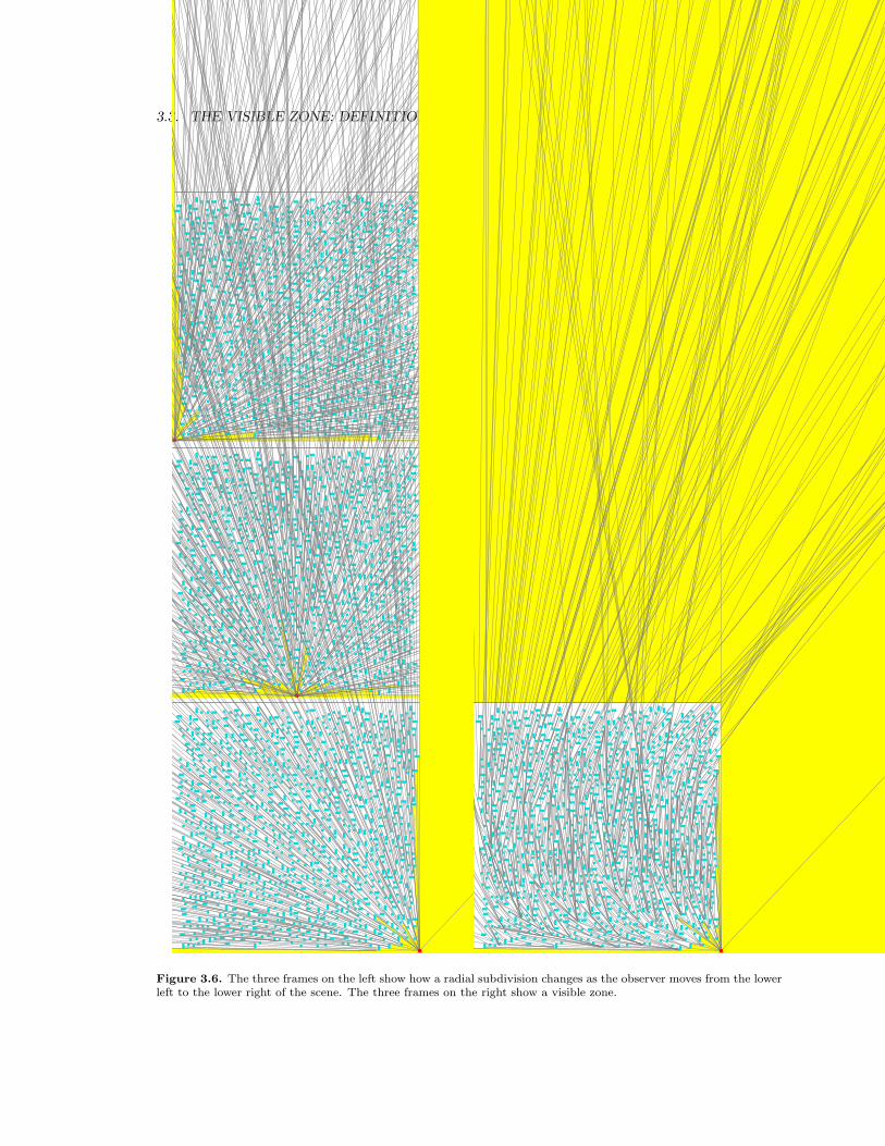
3.3. THE VISIBLE ZONE: DEFINITION AND KINETIC ALGORITHM 19
Figure 3.6. The three frames on the left show how a radial subdivision changes as the observer moves from the lowerleft to the lower right of the scene. The three frames on the right show a visible zone.

20 CHAPTER 3. STATIC OBJECTS: THE VISIBLE ZONE
3.3.2 Kinetic Maintenance of the Visible Zone
The top level of the kinetic algorithm for maintaining the visible zone is just like the algorithm
for maintaining the radial subdivision: 1) initialize the tangent segments using a radial sweep, 2)
construct an event heap, and 3) process required updates in time order. The major differences
are found in how the event times are computed and how the updates are made. In particular,
computing an event time requires a local search among nearby tangent segments, and updates may
require multiple elementary steps.
Computing Event Times
As the observer moves, the tangent segments attached to the observer also move. Unattached tangent
segments, however, do not have to move with the observer in the visible zone, and therefore do not
trigger kinetic updates. The only event times that need to be computed are for tangent segments
attached to the observer.
One case in which a tangent segment t must change due to observer movement is when two
tangent segments that are both attached to the observer are brought together (see Figure 3.7 where
Xright and Yright momentarily coincide). This case occurs exactly when an object ceases to be
visible (or at least ceases to be visible in a particular neighborhood). Identifying the event time
involves the same procedure as used in maintaining the radial subdivision: a line l tangent to the
two tangent objects is identified, and the time at which the observer crosses this line is computed
as the event time.
X
pY Y
X
Figure 3.7. As the observer moves, two neighboring tangent segments attached to the observer become momentarilycollinear, thus requiring an update to their combinatorial descriptions.
The other case that triggers an event is when an object first becomes visible, at least in a given
neighborhood (see Figure 3.8). In this case, a tangent segment t connected to the observer will soon
change its forward object. The question that needs to be answered to compute the event time is:
What object, other than the tangent object of t, is responsible for this change in visibility? That is,
what is the second object defining the line l whose crossing determines the event time?
In a visible zone, unlike the radial subdivision, the answer to this question is not always available

3.3. THE VISIBLE ZONE: DEFINITION AND KINETIC ALGORITHM 21
simply by examining the immediate neighbors of t. For example, in Figure 3.8, the object that will
first become visible as the observer moves to the right is A, but the neighbor of t in that region is
Bright, not Aright. However, Aright is not very far away: it is incident to the forward object F of t.
As will be shown in section 3.5.2, it will always be true that the second object responsible for this
type of event will be connected to the forward object by some tangent segment. The procedure for
computing the event time is to search among the objects connected to F by at least one tangent
segment, and find the object among this set of objects that will cause an event first. This set of
objects includes those connected to F by the opposite end of a tangent segment: back objects, as
well as tangent objects of tangent segments, must be included. The complexity of this search is
proportional to the number of tangent segments connected to the forward object of t.
F
A
B
T
F
A
B
T
(a) (b)
Figure 3.8. Locating the appropriate object for the next event associated with tangent segment Tright involvessearching among the objects connected to its forward object F . The frames above show the initial radial subdivision(a), and the visible zone just before the event (b). Some tangent segments have not been drawn, for clarity.
Visibility Updates and Cascading Elementary Steps
Unlike the radial subdivision, the visible zone does not require updates except when the list of visible
objects changes. However, a single update to a visible zone may be more costly to compute than
a single update to a radial subdivision. As with event time computations, there are two cases. In
the first case (see Figure 3.7), two tangent segments attached to the observer become aligned, and
all that is needed for the update is one elementary step between them (in addition to updating the
event heap).
In the second case, a single change in visibility may require multiple elementary steps (see Figure
3.9). Elementary steps may be dependent on each other; one elementary step may be required in
order for another to take place. The general update procedure for changes in visibility involves
identifying where an elementary step needs to be applied, and either applying that elementary step
right away, or recursively finding another elementary step which must be applied first.
Perhaps the easiest way of describing the steps involved in such an update is by example. Consider
the sequence depicted in Figure 3.9. As the observer moves to the right, the tangent segment Cright

22 CHAPTER 3. STATIC OBJECTS: THE VISIBLE ZONE
turns counter-clockwise about its tangent object C, until Cright becomes tangent to the left side
of A. At that moment, the combinatorial description of Cright needs to change. In order to make
this change, Cright needs to undergo an elementary step with Aleft. In order to bring Aleft into
alignment with Cright, however, Aleft must be turned so far counter-clockwise that its combinatorial
description changes along the way.
As Aleft turns counter-clockwise about A, it needs to update its forward object twice, by means
of elementary steps with Bleft and Dright, respectively. The precise geometric locations of Bleft and
Dright after the elementary step are not important: what matters is the combinatorial description of
each tangent segment, and this description does not have position or angle information. For illustra-
tion purposes, however, we choose some angle that is consistent with the combinatorial information,
so that for example Bleft is shown connected to A, rather than C in the second frame. After these
two elementary steps, Aleft is in a position where it can undergo an elementary step with Cright.
Once the elementary step between Aleft and Cright is applied, the observer can continue moving
to the right, and the tangent segments connected to the observer correctly reflect the list of visible
objects. The various elementary steps described in this update would have occurred earlier if a radial
subdivision were being maintained; the ‘lazy’ approach of the visible zone avoided these elementary
steps until they were necessary.
The recursive update procedure involves finding the next elementary step that a given tangent
segment must undergo as it turns in a particular direction about its tangent object. The procedure
for computing event times described in section 3.3.2 did more than compute a particular event time:
it also identified what second tangent object (and what side of the second object) would be involved
in an event. The event-finding procedure thus identifies the tangent segment needed for the final
elementary step of the recursive visibility update procedure.
A similar but more general procedure is needed for identifying the next elementary step of a
tangent segment t that is not attached to the observer. As will be shown in section 3.5.2, it is
sufficient to consider all the objects connected to the forward and back objects of t by tangent
segments. Let F and B be the forward and back objects of t, respectively. Let SF and SB be the
objects connected by tangent segments to F and B, respectively. To find the next elementary step
for t, each object of SF and SB is examined to see how far t must turn before becoming tangent to
it. (For the sake of constant factor speed-ups, it is possible to examine only those objects on the
relevant side of the tangent segment, and the calculation of turn angles only need be applied to one
of the sides of such an object.) The next elementary step will be determined by the object requiring
the smallest turn.
The correctness of this recursive procedure depends on its termination: in searching for a tangent
segment at which we can perform an elementary step, we must not get into a cycle. Conditions under
which termination is guaranteed will be described in section 3.5.4, but for now we simply assert that
as long as a tangent segment turns toward the position it would occupy in a radial subdivision

3.3. THE VISIBLE ZONE: DEFINITION AND KINETIC ALGORITHM 23
D B
A
CAs the observer moves, the tangent segment Cright be-comes tangent to A. In order to perform an elementarystep, the segment Aleft must be rotated.
D B
A
C
In order to rotate Aleft, we perform a “left-left” elemen-tary step on Aleft and Bleft.
D B
A
C
We continue rotating Aleft, and perform a “right-left” el-ementary step on Aleft and Dright.
D B
A
C
We are finally able to complete the “left-right” elementarystep on Cright and Aleft. The observer is now able to seebetween A and C to D.
Figure 3.9. A recursive cascade of elementary steps.

24 CHAPTER 3. STATIC OBJECTS: THE VISIBLE ZONE
(noting that, in the extreme, it may appear to have turned all the way around its tangent object
and so may need to be unwound), the procedure above is guaranteed to terminate correctly.
Additional Event Updates
An implementation detail in the procedures for identifying elementary steps involves computing
how far a tangent segment must turn about its tangent object before it becomes tangent to a given
second object. The angle of a tangent segment t is the angle formed by the supporting line of t and
a fixed referent (such as the x-axis). The angular difference between two positions can be used to
measure the amount that a tangent segment turns about its tangent object. In comparing which of
two objects will first require a change in the combinatorial description of t, we compare two angular
differences.
Computing angular differences is faster if, as the tangent segment t turns about its tangent object
T , t is always tangent to the same vertex of T . In many cases, an elementary step will require t to
turn just a little, and the tangent vertex will not change. In order to take advantage of this fact,
we can add a new field to the combinatorial description of a tangent segment which specifies the
current tangent vertex.
Keeping track of the current tangent vertex can speed up angle difference calculations, but, on
the other hand, new events are required to keep this information current. A sliding event occurs
when a tangent segment shifts from one tangent vertex to another (see Figure 3.10). Note that this
event type is not required: it is a practical acceleration technique that may not always be important.
Figure 3.10. A tangent segment slides from one vertex to another. Such sliding motions may also occur as tangentsegments attached to the observer change angle.
In conclusion, a kinetic algorithm for maintaining the visible zone is very similar to a kinetic
algorithm for maintaining a radial subdivision, but with slightly more complex event-time calcula-
tions and updates. In preparation for extensions into 3D, the next section considers modifications
to the visible zone that go beyond those required for observer motion.
3.4 The Visible Zone: Query Structure
Many visibility algorithms make use of some type of ray query at a low level. For rays originating
with the observer, a visible zone provides an optimal query structure, or at least the raw ingredients

3.5. THE VISIBLE ZONE: COMBINATORIAL PROPERTIES 25
for such a structure, in the list of tangent segments connected to the observer. In some circumstances,
such as with partially transparent objects, it may be important in addition to allow ray queries from
the observer to pass through some objects while still reporting all objects intersected. An extended
ray query is a ray whose origin lies anywhere in the plane, whose supporting line passes through
the observer, and whose termination criteria may permit passing through more than one object.
The radial subdivision appears ideally suited for such extended ray queries. Processing an ex-
tended ray query r in a radial subdivision would proceed as follows. Suppose r originates in a
particular cell C of the subdivision. Assuming without loss of generality that r is directed away
from the observer, the next object hit by r is the object on the far side of C from the observer. If r
passes through this object A, then the next cell reached by r is among those cells connected to the
far side of A, and the same procedure can be recursively invoked to identify the remaining objects
intersected by r. The extended ray query thus involves a traversal of only as many cells of the radial
subdivision as objects intersected by r. However, as noted earlier, the radial subdivision may be
expensive to maintain if the observer begins to move.
The same query described above may be made using a visible zone, with a slight modification,
as follows. Any tangent segment can be turned, with the help of cascading elementary steps, into
alignment with the current position of the observer. The visible zone can be modified to resemble the
radial subdivision in the neighborhood of a query ray as needed. For example, at the moment when
we are about to search among the cells on the far side of a polygon P for the next cell to contain the
query ray, we first ‘straighten’ all the tangent segments connected to P so that they are aligned with
the observer. This straightening operation can be accomplished iteratively, by starting with the left
or right tangent segment of P , searching for a neighbor t that has not been straightened, turning t
until it is aligned with the observer, and repeating until all attached tangent segments are aligned
with the observer. A similar approach can be used to straighten segments in the neighborhood of a
point in free space. An example of shooting an extended ray into the visible zone is shown in Figure
3.11. The visible zone has been changed near the ray, but not far away from it. Thus the visible
zone provides support for extended ray queries, without all the overhead of maintaining a radial
subdivision for a moving observer.
3.5 The Visible Zone: Combinatorial Properties
The properties of the visible zone, including the correctness of the procedures described above,
derive from properties of the visibility complex. This section is more easily followed if the reader is
already familiar with the visibility complex (see [PV96a]), though some definitions will be included
here for completeness. In the first subsection below, the visible zone is redefined formally with
respect to the visibility complex and elementary steps are also situated in this context. The second
subsection demonstrates the correctness of the angular limit finding procedure described above.
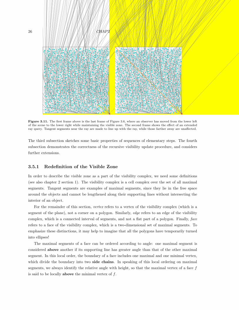
26 CHAPTER 3. STATIC OBJECTS: THE VISIBLE ZONE
Figure 3.11. The first frame above is the last frame of Figure 3.6, where an observer has moved from the lower leftof the scene to the lower right while maintaining the visible zone. The second frame shows the effect of an extendedray query. Tangent segments near the ray are made to line up with the ray, while those farther away are unaffected.
The third subsection sketches some basic properties of sequences of elementary steps. The fourth
subsection demonstrates the correctness of the recursive visibility update procedure, and considers
further extensions.
3.5.1 Redefinition of the Visible Zone
In order to describe the visible zone as a part of the visibility complex, we need some definitions
(see also chapter 2 section 1). The visibility complex is a cell complex over the set of all maximal
segments. Tangent segments are examples of maximal segments, since they lie in the free space
around the objects and cannot be lengthened along their supporting lines without intersecting the
interior of an object.
For the remainder of this section, vertex refers to a vertex of the visibility complex (which is a
segment of the plane), not a corner on a polygon. Similarly, edge refers to an edge of the visibility
complex, which is a connected interval of segments, and not a flat part of a polygon. Finally, face
refers to a face of the visibility complex, which is a two-dimensional set of maximal segments. To
emphasize these distinctions, it may help to imagine that all the polygons have temporarily turned
into ellipses!
The maximal segments of a face can be ordered according to angle: one maximal segment is
considered above another if its supporting line has greater angle than that of the other maximal
segment. In this local order, the boundary of a face includes one maximal and one minimal vertex,
which divide the boundary into two side chains. In speaking of this local ordering on maximal
segments, we always identify the relative angle with height, so that the maximal vertex of a face f
is said to be locally above the minimal vertex of f .

3.5. THE VISIBLE ZONE: COMBINATORIAL PROPERTIES 27
The tangent segments of the radial subdivision are related to each other in the visibility com-
plex as follows. Let R be the set of all maximal segments whose supporting lines pass through the
observer. Then R includes the tangent segments of the radial subdivision. Thus, the maximal seg-
ments of R together constitute a curve through the space of maximal segments, whose intersections
with edges are exactly the tangent segments of the radial subdivision. Intuitively, R is analogous
to a curve drawn on the plane through an arrangement of lines, where we mark the intersections of
the curve with these lines and focus on the edges containing these intersections.
The exact angle of a tangent segment often does not matter, since the combinatorial description
of a tangent segment does not require it. Thus, the curve R is part of an equivalence class of curves
through the visibility complex, which all intersect the same set of edges of the visibility complex.
The following definition follows the terminology used in the original topological sweep paper [EG86],
this time applied to the visibility complex instead of an arrangement of lines.
Definition 1: A cut is a set of edges (called cut edges) with the property that, for any face f
with a cut edge on its boundary, there is exactly one cut edge on each of the side chains of f .
A cut is a slight generalization of the anti-chain topological sweep structure defined in [PV96a].
We also use a slightly different definition for the visibility complex than used previously (our maximal
segments, though oriented, are not affected if the angle is changed by 2π). The zone of a cut is the
set of faces (called zone faces) with cut edges on their boundaries. The perspective cut is the
set of edges containing the tangent segments of the radial subdivision. In order for this definition to
make sense near the observer, the observer is considered to be a polygon that has been shrunk down
to infinitesimal size without destroying the local combinatorial structure of the visibility complex.
The tangent segments that connect to the observer are then considered to belong to edges of the
visibility complex that have been reduced to an infinitesimal extent. Let us call these special edges
the visible edges. The perspective cut captures the notion of the freedom of (most) tangent
segments to move around, possibly intersecting each other as segments in the plane, without losing
the underlying combinatorial information.
The number of edges incident to any given vertex is always four. In a topological sweep of an
arrangement of lines, or of the visibility complex, a cut can be modified incrementally:
Definition 2: An elementary step is an operation by which a cut is changed, by removing two
cut edges that share a vertex, and replacing them with the other two edges incident to the vertex.
An elementary step is considered to go up if it involves replacing edges below a vertex with those
above, or down if it goes the other way. A cut never contains edges both above and below a vertex,
since they would both lie on a single side chain of a face.
Lemma 3.5.1. The set of edges c1 obtained by applying an elementary step to a cut c0 is also a
cut.
Proof: Let e1 and e2 be the lower edges of v, and let e3 and e4 be the upper edges of v. The lower
edges are together adjacent to several faces:

28 CHAPTER 3. STATIC OBJECTS: THE VISIBLE ZONE
Figure 3.12. An abstract depiction of an elementary step, where the cut moves up or down over a vertex of thevisibility complex by substituting two new cut edges.
1) a shared face, fmin, whose maximal vertex is v. Thus the new cut will not include any edges
from either side chain of fmin.
2) two or more other faces adjacent to e1 or e2. For each of these faces, v is not the maximal
vertex, since only one face has maximal vertex v. Let f be one of these faces, which has a lower
edge on a side chain. One of the edges above v is on the same side chain of f as the edge below v.
Thus the number of edges on that side chains remains unchanged.
The upper edges are also adjacent to some number of faces, most of which have already been
examined. The remaining face, fmax, has v as the minimal vertex, and also has the new edges on
opposite side chains. In summary, all the requirements of a cut are still met by c1. ¤
Definition 3: A visible zone is the zone of any cut obtainable by applying elementary steps
to the perspective cut, such that the visible edges always remain in the cut.
A visible zone is a linear substructure of the visibility complex. The definition of the visible zone
given in the earlier part of this chapter is a particular representation for the visible zone, which
could also be represented in other ways. A visible zone captures the combinatorial information of
the visible set, as well as a set of relationships extending to all objects of the scene. It can be
visualized as a quasi-spatial subdivision via tangent segments or as a sort of topological line through
the visibility complex. The latter is useful for establishing its properties, as we will see below.
3.5.2 Correctness of the Event-Finding Procedure
In section 3.3.2, we claimed that the object responsible for the next elementary step of a given
tangent segment t could be found among those objects connected to the forward and back objects
of t by tangent segments. The procedure for calculating event times of section 3.3.2 made a similar
claim, but for the special case where only changes in the forward object were to be considered.
One approach to proving these claims is to consider how various faces in the visibility complex are
connected to each other.
Consider the three cases depicted in Figure 3.13, where a tangent segment Tright turns counter-
clockwise about its tangent object T . In the first case (Figure 3.13a), Tright will become tangent
to the forward object F before it becomes tangent to any other object. In this case, finding the

3.5. THE VISIBLE ZONE: COMBINATORIAL PROPERTIES 29
object responsible for the next elementary step is trivial, since F is referenced in the combinatorial
description of Tright.
F
T
B
A
F
T
B
A
F
T
B
(a) (b) (c)
Figure 3.13. Cases for determining the next elementary step as the tangent segment Tright turns counter-clockwiseabout T .
In Figure 3.13b, as Tright turns counter-clockwise, Tright first becomes tangent to an object A
that lies to the left of Tright. It is not easy to draw faces of the visibility complex directly in this
type of planar diagram, so instead of drawing a whole face, we will instead draw one of the maximal
segments that makes up a face, and refer to the face containing that maximal segment. In particular,
let f be the face that contains the maximal segment parallel to and just to the left of Tright as shown
in Figure 3.14a. The vertex of the elementary step we seek is the maximal vertex (by local angle)
of the face f .
In Figure 3.13c, as Tright turns counter-clockwise, Tright first becomes tangent to the nearest
small object A. Let g be the face containing the segment parallel to and just to the right of Tright
shown in Figure 3.14b. In this case, the vertex of the elementary step we seek to identify is the
maximal vertex of g. In all three cases of Figure 3.13 (and in any case), the object responsible for
the next elementary of Tright is one of the objects tangent to the maximal vertex of one of the faces
of the visibility complex adjacent to Tright.
A
F
T
B
A
F
T
B
(a) (b)
Figure 3.14. Segments defining the faces f and g next to the tangent segment Tright.
Recall that a face of the visibility complex that contains a cut edge along the boundary is called
a zone face. The proof of the following lemma is given in Appendix A:
Lemma 3.5.2 (Zone Propogation). A face immediately below (according to angle) the maximal
vertex of a zone face is itself a zone face.

30 CHAPTER 3. STATIC OBJECTS: THE VISIBLE ZONE
In particular, the face f2 containing the segment shown in Figure 3.15a, whose angle is just below
the angle of the vertex we seek, necessarily has a cut edge along its boundary. Similarly, the face g2
containing the segment shown in Figure 3.15b, with a slightly lesser angle than the vertex, also has
a cut edge along its boundary. Any maximal segment on the boundary of a face connects to the two
objects joined by maximal segments on the interior of the face. Thus the object A in Figures 3.14
and 3.15 is in each case necessarily connected to F or B by means of at least one tangent segment,
and the procedures described in sections 3.3.2 and 3.3.2 for finding objects involved in elementary
steps are correct.
A
F
T
B
A
F
T
B
(a) (b)
Figure 3.15. Segments belonging to two faces f2 and g2 just below the vertex defining the next elementary step. Asusual, this vertex is a maximal segment, not a vertex of a polygon.
3.5.3 Sequences of Elementary Steps
The correctness of the recursive cascading procedure depends on the existence of certain sequences
of elementary steps. More generally, the space of all possible visible zones for a given scene at a
given moment of time can be described with using terminology associated with these sequences. The
treatment of this topic in the following paragraphs will be at a high level, since many of the detailed
proofs do not provide any useful intuition. We begin with some important definitions and properties
for these sequences, and then examine the implications of observer motion.
Minimum Length Sequences
To transform one cut into another, one or more elementary steps may be applied, each of which
moves the cut locally up or down. Although many of the definitions and properties in this section
apply to any cut, we will always assume the cut is associated with a visible zone. An elementary step
(or step, for short) can be represented by a vertex, since the direction of the step is implied by the
location of the cut. A sequence of steps can be represented by a sequence of vertices v1, v2, . . . , vn.
Two cuts are connected if there is a sequence taking one to the other.
Two consecutive steps in a sequence over the same vertex are called a redundant pair, since
their effects on the cut cancel each other out. When a sequence contains a redundant pair, removing
this redundant pair from the sequence is in some sense a trivial adjustment of the sequence. Also,

3.5. THE VISIBLE ZONE: COMBINATORIAL PROPERTIES 31
if two consecutive steps of a sequence are independent, that is if they affect different parts of the
visibility complex, then transposing their order in the sequence is also in some sense a trivial change.
Such a transposition is called an allowable transposition.
Definition 4: Two sequences of steps T1 and T2 that both transform a cut z1 into another cut
z2 are equivalent (T1 ∼ T2) if by allowable transpositions in the order of steps, and the removal of
redundant pairs, T1 and T2 can be reduced to the very same sequence.
One example of when two steps in a transformation sequence can be transposed is the case of a
pair of non-redundant consecutive steps with opposite directions. We examine this case in detail;
the analysis for many other properties is similar in form. Suppose vi and vi+1 are the vertices of
two consecutive steps, which are upward and downward, respectively. The vertices vi and vi+1 are
distinct, by non-redundancy, and so the only way for these two elementary steps to have anything
in common is to share an edge. However, just after the step across vi, an edge above the vertex vi is
a cut edge (by the operation of the elementary step), and just prior to the step across vi+1, an edge
below vi+1 is not a cut edge, so such an edge cannot be shared. Again, just after the step across
vi, an edge below the vertex vi is not a cut edge, whereas an edge above the vertex vi+1 is a cut
edge, so such an edge cannot be shared either. Therefore an upward elementary step can always be
transposed with a downward elementary step next to it in the sequence, provided that these two do
not form a redundant pair.
A unidirectional sequence has all upward steps, or all downward steps. Thus any sequence can
be reduced to a concatenation of two unidirectional sequences, with no vertices shared in common
between their respective steps. This reduced form is called a non-redundant sequence.
In the definition of the visible zone, we required certain cut edges to remain in the cut, regardless
of which sequence was applied. A general mechanism for specifying restrictions on sequences is to
specify some set of vertices (the restricted vertices) that are not allowed to appear in the steps
of any sequence. These sequences are then called restricted sequences.
All restricted sequences connecting a given pair of cuts turn out to be equivalent. A restricted
sequence cannot have an arbitrarily large number of steps, because it would eventually have to cross
a restricted vertex. For any cut, all upward (resp. downward) restricted sequences of maximal length
are equivalent. In a space of connected cuts connected by restricted sequences, there is a unique
maximum cut, obtained by applying the longest possible upward restricted sequence.
The central theorem of this subsection is as follows.
Theorem 3.5.3 (Unique Minimum). Let z be a cut, let V be a set of vertices, let v be a vertex
not in V , and let T be the set of all non-redundant sequences of z restricted by V that have exactly
one upward step over v. Then there exists a minimum length sequence T of T that occurs as a
prefix to all the other sequences of T , up to allowable permutations in the order of steps.
The proof of this theorem proceeds by induction on minimum sequence length, and makes re-
peated use of the uniqueness (up to equivalence) of a sequence linking one cut to another.

32 CHAPTER 3. STATIC OBJECTS: THE VISIBLE ZONE
A minimum length sequence T has several interesting properties, including the following: if T
includes a step over a vertex w, then there is no other step of T over w. Thus to move the cut to
a desired location of the visibility complex, if this location can be described as being on “the other
side” of a particular vertex, then there exists a single most efficient sequence for doing so, and this
sequence will never cross any vertex twice. It is this sequence which is discovered by the cascading
algorithm given earlier.
3.5.4 Effect of Observer Motion
The problem of maintaining a cut then reduces to determining whether its connectivity to other
cuts can be negated by the motion of the observer. We observe that the visibility update algorithm,
if it terminates, will turn tangent segments in only one direction about their tangent objects.
To prove that the visibility update algorithm terminates correctly, we apply the properties de-
veloped for sequences. In particular, we would like to know whether the zone of a cut remains a
visible zone as the observer moves, to ensure that the space of connected cuts never collapses. Let
C be a visibility complex just before a visibility event, and let C ′ be the new visibility complex
just afterwards. We also will assume the change in visibility is non-degenerate (e.g. the observer is
not allowed to pass through a point where two vertices intersect.) To use the above terminology on
sequences, a visible zone can be defined as the zone of a cut connected to the perspective cut via a
restricted sequence, where the restriction refers to the upper and lower vertices of the visible edges.
Lemma 3.5.4. Let z be the cut associated with a visible zone in C, and z′ the corresponding cut
in C ′. Then z′ is also connected to the perspective cut.
Proof: (Sketch) In order to examine the structure of the visibility complex in the neighborhood of
the observer, recall that we start with a finite-sized observer, which is then shrunk down. The finite-
sized observer crosses the line l corresponding to a visibility event in three steps: the observer first
reaches l at a point along the boundary of the observer, then eventually the center of the observer
(from which visibility is computed) crosses l, and finally the observer ceases to have any intersection
with l. It is only at the second of these three steps, when the center of the observer crosses l, that
the recursive visibility update algorithm is applied. The first and last of these steps are when the
combinatorial structure of the visibility complex changes. The vertices of the visibility complex that
are affected as a result of this triple tangency between the (finite) observer and two scene objects
are so close to a restricted vertex that they cannot be a part of the sequence of elementary steps
joining z or z′ to the perspective cut. ¤
Since we are assured that some sequence exists to convert z into z′, we know also that the
visibility update algorithm identifies the shortest such sequence, and thus will terminate correctly.

3.6. THE VISIBLE ZONE: WORST CASE COMPLEXITY 33
3.6 The Visible Zone: Worst Case Complexity
The construction of the initial visible zone consists of the construction of the radial subdivision, thus
requiring O(n log n) time with a low constant factor.
One of the most important maintenance costs in a kinetic algorithm of this type is the cost
of changing the motion of the observer. In a real-time fly-through, for example, the motion of the
observer may change often. In the kinetic algorithm above, a change in the flight plan of the observer
requires a recomputation of all the event times that involve the observer. These event times are all
associated with tangent segments connected to the observer, and so the number of these events in
the event heap is proportional to the size of the visible set. When the observer changes its motion,
only these event times need to be recomputed, in constant time each, for a total cost proportional
to the size of the visible set v. A more sophisticated approach using dynamic convex hulls can
reduce this dependence to O(polylog v) (see [BGH99]) while still retaining the overall approach of
the visible zone.
When the observer moves along a single trajectory describable by a constant degree pseudo-
algebraic expression, the time complexity can be expressed in terms of the number of elementary
steps. Also, along such a trajectory, the angle of a tangent to a given object that passes through the
observer will evolve in a fairly simple manner, switching between increasing and decreasing only a
constant number of times. It can be shown that, during a cascade of elementary steps, the tangent
segments always turn ‘toward’ the observer, or more precisely they turn toward the angle they would
have in a radial subdivision, and thus the number of elementary steps is bounded by O(k), where
k is the size of the visibility complex. The size k is also an upper bound on the total number of
changes in visibility that may occur along such a path, and may be as low as linear. Unfortunately,
this bound is still loose: even the radial subdivision requires no more than O(k) elementary steps.
A more refined analysis, based on bounding the size of cascades in terms of a specialized scene
descriptor, can show that in some cases the number of elementary steps per cascade is at most a
constant factor larger than the largest number of objects visible to a point observer at any time.
However, the constant factors given are exponential in the scene descriptor.
In practice, for roughly uniformly distributed scenes, the constant factors involved may be quite
low. For example, in a simulation of a linear movement of the observer through a scene of 100,000
randomly placed objects, where the average number of objects visible at any given time to a point
observer was approximately 74, the average number of elementary steps involved in an update was
approximately 39.
The visible zone kinetic algorithm also differs from an approach that simply triangulates the
space between objects initially and then queries this static triangulation over time. Such a query-
based approach might need to perform an expensive query many times, thus limiting the efficiency of
the method when, for example, the observer changed direction often. Instead, the visible zone acts
as a sort of lazy approximation to the radial subdivision, changing its combinatorial structure just

34 CHAPTER 3. STATIC OBJECTS: THE VISIBLE ZONE
enough at each update to maintain a certain global consistency among the various tangent segments.
At any time, any part of a visible zone can be made to look just like the radial subdivision, but it
is not necessary to enforce the similarity at all times or places.
3.7 Extension of the Visible Zone to Moving Objects
In this chapter, we have described a simple scalable solution, under certain assumptions on the
input geometry, to the problem of maintaining the visible set of a moving observer in the plane. The
visible zone takes linear space and is based on the familiar elements of a trapezoidal subdivision.
Its simplicity makes it extensible in a variety of ways, including the capability of handling extended
ray queries for use in 3D approaches. The visible zone is a direct application of properties of the
visibility complex to a dynamic visibility problem.
Extending the maintenance of the radial subdivision to a scene of moving objects, as well as a
moving observer, is fairly straightforward (see [NT99a]). It is natural to seek to extend the visible
zone similarly. Various non-trivial modifications to the event-finding and update procedures do exist
to allow such an algorithm to work, and we have even implemented such an algorithm. Unfortunately,
in an extremely special case, the recursive procedure for cascading elementary steps can fall into an
infinite loop. A situation where this case could conceivably occur is shown in Figure 3.16. It is not
clear how to produce this situation starting from a radial subdivision and moving objects around,
but it may nevertheless be possible, perhaps with the help of very small objects circulating around
those shown in Figure 3.16.
Figure 3.16. The scene above depicts a visible zone with the observer in the center. If the topmost object is movedup a distance equal to a tenth of its height, no tangent segments will be disturbed, but the resulting configuration nolonger represents a visible zone: it is no longer connected via elementary steps to the radial subdivision.
This special case was discovered through our work on generalizing the proofs of correctness
summarized above. A fix for this case is to have the recursive procedure detect cycles and make
two ‘illegal’ changes to the cut that cancel each other out, leaving a valid visible zone as a result.

3.7. EXTENSION OF THE VISIBLE ZONE TO MOVING OBJECTS 35
However, the procedures involved are not simple, and the complexity analysis appears yet more
difficult, even when such a special case is assumed not to occur.
Maintenance of visibility for moving objects thus appears, at least in the context of maintenance
of the visible zone, to be considerably more difficult to handle in general than having just the observer
move. An algorithm developed specifically for that situation – maintaining visibility among moving
objects with the same goals for scalability – will be the subject of chapter 4.

36 CHAPTER 3. STATIC OBJECTS: THE VISIBLE ZONE
Chapter 4
Moving Objects: The Corner Arc
Algorithm
How can visibility be maintained for a point observer amid a set of moving objects? According to a
recent survey of visibility [COCS00], relatively little has been discovered about visibility algorithms
for dynamic scenes. When a large fraction of the scene objects are moving continuously, maintain-
ing standard scene hierarchies can involve complex and time consuming update operations. Even
characterizing the efficiency of such approaches appears to be difficult.
Instead of using a scene hierarchy to accelerate visibility computations, chapter 3 described a
method by which the shape of the visibility polygon is represented within a spatial subdivision, and
this shape is maintained within the spatial subdivision as the observer moves. The general approach
of embedding the shape of the visibility polygon within some spatial subdivision has important
benefits. In particular, the cost of a change in visibility may be low, even when objects involved in
such a change in visibility are far from the observer.
A different spatial subdivision, called a pseudo-triangulation [PV96a], can be used to partition
the space between moving convex objects [ABG+00]. Although a pseudo-triangulation cannot embed
the shape of a visibility polygon exactly, an approximation can be constructed by means of ‘corner
arcs’. This approximation provides the benefits of representing the shape of the visibility polygon,
and allows any number of moving objects to be handled efficiently.
The corner arc algorithm uses linear space and has optimal computational complexity (up to a
polylogarithmic factor) for an important class of scenes of moving objects. Prior to the development
of the corner arc algorithm, it was not known whether this level of efficiency could be achieved
by any visibility maintenance algorithm. This result also implies that the asymptotic complexity of
maintaining visibility among moving objects is the same (up to a polylogarithmic factor) as visibility
maintenance among static objects, again for an average case setting.
37
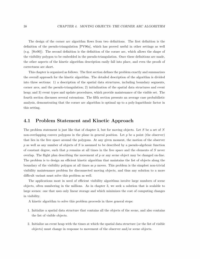
38 CHAPTER 4. MOVING OBJECTS: THE CORNER ARC ALGORITHM
The design of the corner arc algorithm flows from two definitions. The first definition is the
definition of the pseudo-triangulation [PV96a], which has proved useful in other settings as well
(e.g. [Str00]). The second definition is the definition of the corner arc, which allows the shape of
the visibility polygon to be embedded in the pseudo-triangulation. Once these definitions are made,
the other aspects of the kinetic algorithm description easily fall into place, and even the proofs of
correctness are short.
This chapter is organized as follows. The first section defines the problem exactly and summarizes
the overall approach for the kinetic algorithm. The detailed description of the algorithm is divided
into three sections: 1) a description of the spatial data structures, including boundary segments,
corner arcs, and the pseudo-triangulation; 2) initialization of the spatial data structures and event
heap; and 3) event types and update procedures, which provide maintenance of the visible set. The
fourth section discusses several extensions. The fifth section presents an average case probabilistic
analysis, demonstrating that the corner arc algorithm is optimal up to a poly-logarithmic factor in
this setting.
4.1 Problem Statement and Kinetic Approach
The problem statement is just like that of chapter 3, but for moving objects. Let S be a set of N
non-overlapping convex polygons in the plane in general position. Let p be a point (the observer)
that lies in the free space around the polygons. At any given moment, the motion of the observer
p as well as any number of objects of S is assumed to be described by a pseudo-algebraic function
of constant degree, such that p remains at all times in the free space and the elements of S never
overlap. The flight plan describing the movement of p or any scene object may be changed on-line.
The problem is to design an efficient kinetic algorithm that maintains the list of objects along the
boundary of the visibility polygon at all times as p moves. This problem is the simplest non-trivial
visibility maintenance problem for disconnected moving objects, and thus any solution to a more
difficult variant must solve this problem as well.
The applications most in need of efficient visibility algorithms involve large numbers of scene
objects, often numbering in the millions. As in chapter 3, we seek a solution that is scalable to
large scenes: one that uses only linear storage and which minimizes the cost of computing changes
in visibility.
A kinetic algorithm to solve this problem proceeds in three general steps:
1. Initialize a spatial data structure that contains all the objects of the scene, and also contains
the list of visible objects.
2. Initialize an event heap with the times at which the spatial data structure (or the list of visible
objects) must change in response to movement of the observer and/or scene objects.

4.2. SPATIAL DATA STRUCTURE 39
3. Repeatedly remove the first event in time order from the event heap, and make the necessary
change in the spatial data structre and/or list of visible objects.
The description of the corner arc algorithm will include a description of the spatial data structure,
computation of event times, and update procedures for maintaining the spatial subdivision.
4.2 Spatial Data Structure
The corner arc algorithm solves the problem of this chapter via three problem transformations, as
follows.
1. Transform the problem of maintaining a list of visible objects into the problem of maintaining
a combinatorial description of the boundary of the visible region by focusing on ‘boundary
segments.’
2. Transform the problem of maintaining boundary segments into maintenance of a topologically
equivalent structure, called a ‘corner arc’.
3. Transform the problem of maintaining corner arcs into a problem of maintaining a particular
spatial subdivision, namely a pseudo-triangulation.
These three transformations introduce the three elements of the data structure, and each of
which will be described in turn.
4.2.1 Definition of Boundary Segments
A kinetic algorithm for maintaining the list of visible objects must process changes to this list as the
changes occur. Changes in visibility always happen along the boundary of the visibility polygon. A
boundary segment is a line segment on the boundary of the visibility polygon that connects two
objects (see Figure 4.1). A boundary segment serves to separate the visible region from the occluded
region of free space. The supporting line of a boundary segment passes through the observer, and
changes in visibility always occur along boundary segments.
Each boundary segment is incident to two objects: one closer to the observer (the tangent
object), and one farther away (the far object). If the data structure for a boundary segment
includes pointers to the tangent and far objects, then the boundary segments implicitly encode the
combinatorial structure of the visibility polygon, including the list of visible objects. Also, if pointers
to all the boundary segments are stored in a balanced tree structure, ray queries from the observer
can be processed in O(log v) time, where v is the number of visible objects. For the remainder of
this chapter, maintenance of the boundary segments is equated with maintenance of visibility.
As the observer and/or scene objects move, the boundary segments also move. As a boundary
segment b moves, b remains tangent to its tangent object, just like one of the tangent segments of
40 CHAPTER 4. MOVING OBJECTS: THE CORNER ARC ALGORITHM
(a) visibility polygon (b) boundary segments
Figure 4.1. The boundary of the visibility polygon shown in (a) consists of an alternating sequence of parts ofobjects boundaries and segments through free space. These segments, shown in (b), are called boundary segments.
chapter 3. However, the far object of b may change (see Figure 4.2), and if it does then this change
will occur when a second object becomes momentarily tangent to b. These tangency events will
be discussed in more detail in section 4.4.1; the key observation to make now is that to maintain
visibility, an event-based algorithm must have a way to compute the event times for tangency events.
=⇒Figure 4.2. An example of a tangency event, where a particular boundary segment moves from one far object toanother.
4.2.2 Definition of Corner Arcs
Computing the tangency event time for a boundary segment b requires the identification of the
second object to which b becomes tangent. In principle, any object of a dynamic scene (except the
tangent object of b) may eventually move to become this second object tangent to b. The corner arc
algorithm chooses a particular object for this calculation as follows.
Let b be a boundary segment with tangent object T and far object F (see Figure 4.3b). Intuitively,
the corner arc of b is obtained by turning b into an elastic band and pulling the end of b along the
far object F , away from the visibility polygon, until it becomes tangent (rather than just incident) to
F . The corner arc is a concave chain of segments and connecting object boundary arcs that begins
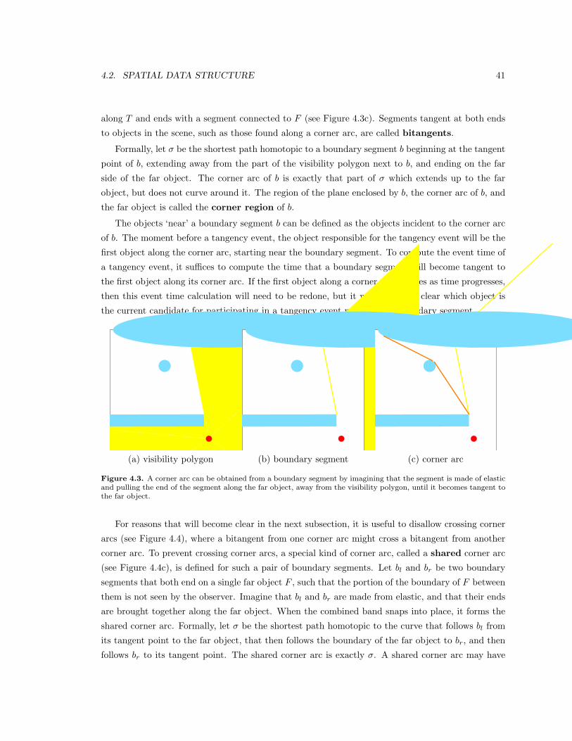
4.2. SPATIAL DATA STRUCTURE 41
along T and ends with a segment connected to F (see Figure 4.3c). Segments tangent at both ends
to objects in the scene, such as those found along a corner arc, are called bitangents.
Formally, let σ be the shortest path homotopic to a boundary segment b beginning at the tangent
point of b, extending away from the part of the visibility polygon next to b, and ending on the far
side of the far object. The corner arc of b is exactly that part of σ which extends up to the far
object, but does not curve around it. The region of the plane enclosed by b, the corner arc of b, and
the far object is called the corner region of b.
The objects ‘near’ a boundary segment b can be defined as the objects incident to the corner arc
of b. The moment before a tangency event, the object responsible for the tangency event will be the
first object along the corner arc, starting near the boundary segment. To compute the event time of
a tangency event, it suffices to compute the time that a boundary segment will become tangent to
the first object along its corner arc. If the first object along a corner arc changes as time progresses,
then this event time calculation will need to be redone, but it will always be clear which object is
the current candidate for participating in a tangency event with a given boundary segment.
(a) visibility polygon (b) boundary segment (c) corner arc
Figure 4.3. A corner arc can be obtained from a boundary segment by imagining that the segment is made of elasticand pulling the end of the segment along the far object, away from the visibility polygon, until it becomes tangent tothe far object.
For reasons that will become clear in the next subsection, it is useful to disallow crossing corner
arcs (see Figure 4.4), where a bitangent from one corner arc might cross a bitangent from another
corner arc. To prevent crossing corner arcs, a special kind of corner arc, called a shared corner arc
(see Figure 4.4c), is defined for such a pair of boundary segments. Let bl and br be two boundary
segments that both end on a single far object F , such that the portion of the boundary of F between
them is not seen by the observer. Imagine that bl and br are made from elastic, and that their ends
are brought together along the far object. When the combined band snaps into place, it forms the
shared corner arc. Formally, let σ be the shortest path homotopic to the curve that follows bl from
its tangent point to the far object, that then follows the boundary of the far object to br, and then
follows br to its tangent point. The shared corner arc is exactly σ. A shared corner arc may have
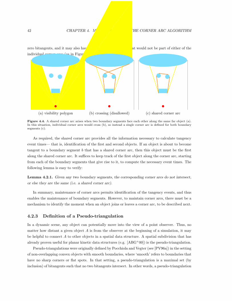
42 CHAPTER 4. MOVING OBJECTS: THE CORNER ARC ALGORITHM
zero bitangents, and it may also have one or more bitangents that would not be part of either of the
individual corner arcs (as in Figure 4.4).
(a) visibility polygon (b) crossing (disallowed) (c) shared corner arc
Figure 4.4. A shared corner arc arises when two boundary segments face each other along the same far object (a).In this situation, individual corner arcs would cross (b), so instead a single corner arc is defined for both boundarysegments (c).
As required, the shared corner arc provides all the information necessary to calculate tangency
event times— that is, identification of the first and second objects. If an object is about to become
tangent to a boundary segment b that has a shared corner arc, then this object must be the first
along the shared corner arc. It suffices to keep track of the first object along the corner arc, starting
from each of the boundary segments that give rise to it, to compute the necessary event times. The
following lemma is easy to verify:
Lemma 4.2.1. Given any two boundary segments, the corresponding corner arcs do not intersect,
or else they are the same (i.e. a shared corner arc).
In summary, maintenance of corner arcs permits identification of the tangency events, and thus
enables the maintenance of boundary segments. However, to maintain corner arcs, there must be a
mechanism to identify the moment when an object joins or leaves a corner arc, to be described next.
4.2.3 Definition of a Pseudo-triangulation
In a dynamic scene, any object can potentially move into the view of a point observer. Thus, no
matter how distant a given object A is from the observer at the beginning of a simulation, it may
be helpful to connect A to other objects in a spatial data structure. A spatial subdivision that has
already proven useful for planar kinetic data structures (e.g. [ABG+00]) is the pseudo-triangulation.
Pseudo-triangulations were originally defined by Pocchiola and Vegter (see [PV96a]) in the setting
of non-overlapping convex objects with smooth boundaries, where ‘smooth’ refers to boundaries that
have no sharp corners or flat spots. In that setting, a pseudo-triangulation is a maximal set (by
inclusion) of bitangents such that no two bitangents intersect. In other words, a pseudo-triangulation

4.2. SPATIAL DATA STRUCTURE 43
can be constructed as follows: 1) choose a bitangent that does not intersect any of the bitangents
previously chosen, 2) repeat until it is no longer possible to find a non-intersecting bitangent. For the
setting of polygons, whose boundaries consist entirely of sharp corners and flat spots, the definition
must be modified slightly to allow bitangents that share an endpoint, but not in such a way that
they would cross if the polygon were viewed as the limit of long sequence of smooth approximating
objects. See Figure 4.5 for examples of allowed and unallowed bitangent choices.
(a) not allowed (b) allowed
Figure 4.5. The requirements for non-intersection of bitangents are formulated as though the polygons were actuallyslightly rounded at the vertices. The rounding would have the effect of causing the bitangents in (a) to cross, andhence is not allowed, whereas in (b) the bitangents would merely move apart, and so both would be permitted in thesame pseudo-triangulation.
The bitangents of a pseudo-triangulation partition the free space around the objects into cells
that are called pseudo-triangles. The boundary of a pseudo-triangle consists of three concave
chains of zero or more bitangents, joined at three cusps.
The immediate relationship between a pseudo-triangulation and a corner arc is that both can
be described using a set of bitangents. To identify objects near corner arcs, we construct a pseudo-
triangulation that includes the bitangents of the various corner arcs, and then consider those objects
along pseudo-triangles next to the corner arcs as being nearby. Such a construction is possible
since no two corner arcs intersect, and by choosing the bitangents of the corner arcs first in the
construction of a pseudo-triangulation T , these bitangents will be guaranteed to form part of T .
T then provides some notion of locality for each corner arc, and for every other geometric element
of the scene. Other approaches to building pseudo-triangulations that include corner arcs will be
described in section 2.
When using a pseudo-triangulation for point visibility calculations, there are at least three options
for the relationship between the point observer and the pseudo-triangulation:
1. the observer is not considered to be an object of the scene as far as the pseudo-triangulation
is concerned, so no bitangents connect to the observer;

44 CHAPTER 4. MOVING OBJECTS: THE CORNER ARC ALGORITHM
Item to be initialized Time complexity
1) Any pseudo-triangulation (preferably one with low-stabbing number) O(N log N)
2) Boundary segments (radial sweep within the pseudo-triangulation) O(vt log t)
3) Corner arcs (applying embedding algorithm to each boundary segment) O(vt log t)
4) Event heap (calculating event times for all event types, and insertingthese into a heap)
O(N log N)
Table 4.1. Sequence of operations for initializing the kinetic data structure. N is the number of objects, v is thenumber of boundary segments, and t is the maximum number of objects along the boundary of pseudo-triangles thatintersect any given ray from the observer.
2. the observer, though only a point, is nevertheless to be considered an object of the scene,
endowed with connecting bitangents; or
3. the observer is a finite object in the scene, and visibility is computed relative to a point on the
interior of this finite object.
Of these various options, the first approach involves the least overhead for an observer that is removed
from the scene and then re-inserted in another place, the second approach is useful for certain
extensions described in section 4.5, and the third approach is probably the easiest to implement.
Any of these options can be used for the corner arc algorithm.
In summary, the spatial data structure of the corner arc algorithm consists of three elements: 1)
boundary segments, which encode the visible objects; 2) corner arcs, which permit events relevant
to boundary segments to be computed; and 3) a pseudo-triangulation, which connects all the ob-
jects and allows events relevant to corner arcs to be computed. The data structures for individual
boundary segments and bitangents record essential combinatorial information. This combinatorial
information includes pointers to tangent objects and neighbors, such as the immediate neighbors of
a bitangent along an object boundary.
4.3 Initialization of the Corner Arc Algorithm
An efficient approach to initialization of the spatial data structure of the corner arc algorithm con-
sists of initializing a pseudo-triangulation first, then using this spatial subdivision to accelerate the
construction of boundary segments and corner arcs (see Table 4.3). This approach to initialization
also allows a given pseudo-triangulation to be re-used if the observer is removed from one location
and inserted into another (if, for example, a user wanted to move the observer suddenly to an en-
tirely different part of the scene). The subsections below describe pseudo-triangulation, boundary
segment, and corner arc initialization routines, respectively.
4.3. INITIALIZATION OF THE CORNER ARC ALGORITHM 45
4.3.1 Initialization of a Pseudo-triangulation
For a scene of N objects, the number of possible pseudo-triangulations is exponential in N . Ini-
tializing a pseudo-triangulation implies choosing a particular pseudo-triangulation among all these
possibilities. A possible choice would be a ‘greedy’ pseudo-triangulation [PV96a] whose initialization
requires O(N log N) time. Another choice is a pseudo-triangulation designed for an arbitrary initial
observer location. If the initial location of the observer is not known at the time of this initialization,
or more broadly if the trajectory of an observer is not known until later, the latter choice will likely
result in more efficient updates.
When a pseudo-triangulation is used for visibility from a point, whether for visibility maintenance
or just for ray queries, the cost of visibility calculations will be related to the number of bitangents
crossed by rays from the observer. The stabbing number of a pseudo-triangulation can be defined as
the maximum number of bitangents intersected by any line segment that lies outside all the objects
(that is, in free space). The problem of devising low-stabbing number triangulations has been
studied for a long time [AF97], and analogous approaches can be devised for pseudo-triangulations.
In practice, if the objects have a relatively uniform size, then an incremental construction algorithm
may be able to achieve a low stabbing number by ordering the insertions in such a way as to mimic
a depth-first traversal of a quad-tree over the scene.
4.3.2 Initialization of Boundary Segments
A radial sweep may be used to construct the initial set of boundary segments at the beginning of
the simulation, just as in chapter 3. Alternatively, given a pseudo-triangulation, it may be more
efficient to apply a radial sweep within the pseudo-triangulation. The cost of the latter strategy
depends on the particular pseudo-triangulation. Let us call the complexity of a pseudo-triangle the
number of bitangents along its sides, and the complexity of a set of pseudo-triangles the sum of the
individual pseudo-triangle complexities. If the complexity of the set of pseudo-triangles intersecting
any given ray from the observer is at most t, and the number of boundary segments is v, then the
cost of initializing all the boundary segments is O(vt log t).
4.3.3 Initialization of Corner Arcs
The corner arcs of the boundary segments can be constructed by iterating over the set of boundary
segments and constructing a corner arc for each boundary segment in turn. Each corner arc will
be represented as a set of bitangents within the pseudo-triangulation. The construction of a corner
arc consists of modifying the pseudo-triangulation locally to include the necessary bitangents. The
method for constructing a corner arc described next not only enables the initialization of corner
arcs, but will also be used for event handling in the on-line portion of the algorithm.
The basic mechanism for modifying a pseudo-triangulation is called a flip [PV96a]. A flip consists

46 CHAPTER 4. MOVING OBJECTS: THE CORNER ARC ALGORITHM
of removing a bitangent from the pseudo-triangulation, and replacing it with the only other bitangent
that can fit in the space thus made available. This flip is analogous to a flip in a triangulation, where
one diagonal of a convex quadrilateral is exchanged for the other diagonal. Unlike a triangulation,
a pseudo-triangulation permits any of the bitangents that are not on the convex hull to be flipped.
Given a particular boundary segment b and pseudo-triangulation T , the corner arc of b can be
embedded in T as follows (see Figure 4.6). Imagine walking away from the observer along b, starting
from the tangent point of b and stopping at the opposite endpoint on the far object F . Along this
trajectory, flip any bitangents encountered in the order that they are reached. Then walk along the
border of F away from the visibility polygon, flipping any incident bitangents, until a bitangent is
found that is directed back toward b. At this time, the corner arc is guaranteed to be complete.
The next two subsections describe the embedding procedure for individual and shared corner arcs
in detail and prove the correctness of this procedure.
(a) initial configuration (b) after ClearSeg (c) after ClearSide
Figure 4.6. A pseudo-triangulation (a) can easily be modified to include a particular corner arc: flip each of thebitangents that intersect the interior of the corner arc region, in the order determined by moving from the tangentpoint of the boundary segment to the far object (b), and then along the far object to the end of the corner arc (c).
4.3.4 Embedding Individual Corner Arcs
Let us begin with an observation about the location of a flipped bitangent:
Lemma 4.3.1. Given a ray r tangent to pseudo-triangle τ such that the origin of r coincides with
its tangent point, let b be the bitangent of τ intersected by r. If b is flipped, the resulting bitangent
b′ does not intersect r, nor does it intersect the interior of the corner arc region.
Proof: Let a1, a2, and a3 be the three side arcs of τ , with p along a1, and b along a2. When b is
flipped to form b′, then b′ crosses where b used to be. Thus b′ is tangent to a1 or a3. If b′ were to
cross r, b′ would be contained entirely inside τ , a contradiction. Therefore b′ cannot cross r.
If b′ were to intersect the corner arc region, then in order to avoid r it would need to be incident
to the forward object. Also, b′ would need to extend a1, rather than a3, to be near the corner arc

4.3. INITIALIZATION OF THE CORNER ARC ALGORITHM 47
region. However, by extending a1 to the forward object, b′ forms the last bitangent of a concave
chain of bitangents from the tangent object to the forward object: b′ is then itself along the corner
arc, and does not intersect the interior of the corner arc region. ¤
Therefore to modify a pseudo-triangulation so that a given boundary segment is enclosed by
a single pseudo-triangle, it is sufficient to flip the bitangents intersected by the boundary segment
one after another starting from the tangent end of the boundary segment. We call this procedure
ClearSeg, since it involves clearing the pseudo-triangulation of bitangents that cross the boundary
segment (compare (a) and (b) of Figure 4.6).
In constructing a pseudo-triangle that contains the boundary segment, the corner arc will some-
times appear as an immediate by-product. Whenever the corner arc region is cleared of all bitangents,
the bitangents of the corner arc are necessarily part of the pseudo-triangulation, by the maximality
of the number of edges in the pseudo-triangulation. In some cases, however, despite clearing the
boundary of the corner arc region along the boundary segment, there may still be a bitangent con-
nected to the far object that intersects the corner arc region (see Figure 4.6 for an example where
this case arises). A procedure similar to ClearSeg, called ClearSide, can be used to finish the
construction of the corner arc (compare (b) and (c) of Figure 4.6), as follows. Iterate over the set of
bitangents connected to the far object, beginning next to the boundary segment, and moving away
from the visibility polygon. For each bitangent, if it is directed away from the boundary segment,
flip it; otherwise, stop, the iteration is complete. Formally,
Lemma 4.3.2. Let t be a boundary segment crossing no bitangents of the pseudo-triangulation.
Let b be the first bitangent encountered tangent to the far object, moving along the boundary of
the corner region away from T . If b is not part of the corner arc of t, then the bitangent b′ obtained
by flipping b does not intersect the interior of the corner region.
Proof: First, if b′ were to intersect t, then by flipping b′, we would get b again, which clearly
intersects the interior of the corner region, thus contradicting the previous lemma. So b′ cannot
intersect t. If b′ were to intersect the interior of the corner region, b′ would have to be tangent to
the far object. But b′ crosses (the location of) b, and b is already tangent to the far object, implying
that b′ would be tangent to the far object, but extending toward t. That is, b′ would then be the
last bitangent on the corner arc, and would not intersect the interior of the corner region. ¤
The combination of ClearSeg and ClearSide is thus guaranteed to embed a corner arc in a
pseudo-triangulation.
4.3.5 Embedding Shared Corner Arcs
Happily, the same tools used to embed individual corner arcs can also be used for constructing
shared corner arcs:

48 CHAPTER 4. MOVING OBJECTS: THE CORNER ARC ALGORITHM
Lemma 4.3.3. A shared corner arc can be constructed by sequentially constructing the two indi-
vidual corner arcs, in any order.
Proof: Let tl and tr be two neighboring boundary segments along the same far object A, for example
as shown in Figure 4.7. Without loss of generality, construct the individual corner arc cr of tr first,
by applying ClearSeg and ClearSide.
Constructing individual corner arcs is clearly sufficient when tl and tr, though neighbors, do
not have a shared corner arc, which would happen if their far object bulges far enough toward the
observer between them. When, however, tl and tr do share a corner arc, then in the process of
applying ClearSeg and ClearSide to tl, there will be a moment when a particular bitangent b of cr
is reached and is about to be flipped (see Figure 4.7).
(a) one boundary segment with corner arc (b) two boundary segments with shared corner arc
Figure 4.7. The construction of a shared corner arc proceeds as though individual arcs are being computed. In (a),the corner arc for the boundary segment on the right is computed. In (b), by the time ClearSeg reaches the cornerarc calculated in (a), the shared corner arc is in place. Some bitangents have been omitted from this figure for clarity.
At that instant, if b were instead an object in its own right, we would have constructed a corner
arc for tl to b (or possibly b plus some part of the boundary of the forward object). Therefore, the
shared arc would necessarily already be in place, and any flips applied during the remainder of the
construction of the individual arc of tl would not disturb it. ¤
4.4 Events and Event Handling
To maintain visibility as the observer and/or scene objects move, a kinetic algorithm calculates the
moment in time at which the combinatorial description of the scene must change, and updates the
spatial data structure appropriately when this time is reached. Particular types of events are used to
maintain each of the three parts of the spatial data structure (see Table 4.4). This section describes
each of the events and event updates in detail, including the methods necessary to compute event
times.

4.4. EVENTS AND EVENT HANDLING 49
Parts of the spatial data structure are maintained by these event typesboundary segments tangency events: shaft, unshaft, peek, and unpeek events
optional: sliding events
corner arcs (in pseudo-triangulation) tangency events: shaft, unshaft, peek, and unpeek events
pseudo-triangulation bitangents pseudo-triangle events: reflex or corner eventsoptional: sliding events
Table 4.2. The types of events used to maintain visibility with corner arcs.
4.4.1 Events for Maintaining Boundary Segments
Let b be a boundary segment tangent to some object T . As the observer and/or scene objects move,
b will appear to turn around T until some combinatorial change in its description becomes necessary.
A tangency event occurs when a scene object other than T becomes tangent to b. Changes in the
visible set occur exactly when tangency events occur.
The event time of a tangency event is determined by the moment at which the observer crosses
a line tangent to its tangent object and the first object along its corner arc. If a boundary segment
has a shared corner arc with no bitangents, no event time calculation is needed (there will not be
an event until there is a corner arc with at least one bitangent). The event time is determined by
the motion of the two objects and the motion of the observer. The equation of motion that needs
to be solved for these events is quadratic in the degree of the three flight plan descriptions, and can
be computed easily for simple linear motion.
Once the event times have been calculated, the events can be placed on the event heap and
processed in time order.
There are four types of tangency events, which we call peek, unpeek, shaft, and unshaft events. In
describing these events, it is useful to distinguish between the two objects that momentarily share a
common tangent through the observer. The near tangent object appears closer to the observer, and
the far tangent object appears farther away, along the affected boundary segment(s). Similarly,
we call the associated boundary segments the near and far boundary segments, according to the
relative distances of their tangent points to the observer.
In a peek event the observer starts to see an object previously hidden by the near tangent object
(see Figure 4.8a). The peek event update must create a new boundary segment on the far tangent
object. An unpeek event requires the reverse operation (see Figure 4.8b): removal of the boundary
segment of the far tangent object. Although it is useful to maintain pointers between neighboring
boundary segments along a common far object, this operation is straightforward and will not be
described in detail.
In a shaft event the observer starts to see between two objects (see Figure 4.9a). The shaft event
update creates a new boundary segment on the far tangent object. This event is potentially the

50 CHAPTER 4. MOVING OBJECTS: THE CORNER ARC ALGORITHM
(a) peek event (b) unpeek event
Figure 4.8. A peek event turns one boundary segment into two boundary segments (a), and an unpeek event reversesthis operation (b).
most expensive update, since it may dramatically increase the penetration of the visibility polygon
into the scene. An unshaft event requires the reverse operation (see Figure 4.9b): removal of the
boundary segment of the far tangent object.
(a) shaft event (b) unshaft event
Figure 4.9. A shaft event also turns one boundary segment into two boundary segments (a), and an unpeek eventreverses this operation (b).
4.4.2 Events for Maintaining Corner Arcs
The events involved in maintaining corner arcs can be divided into two categories: 1) those associated
with changes in visibility, that is the tangency events, and 2) those associated with maintaining a
valid pseudo-triangulation, such as when an object joins or leaves the corner arc of a given boundary
segment. We examine the tangency events first.
At a high level, the event handling for each of the four tangency event types is just an application
of the embedding procedure described for initialization, since whenever a particular corner arc is
needed, the embedding procedure can be called to construct the corner arc. The figures in this
section depict slightly more complex situations for each of the tangency events than were shown
in describing the effect on boundary segments, since the most complex updates of corner arcs are
associated with shared corner arcs. If two boundary segments have a shared corner arc, then we

4.4. EVENTS AND EVENT HANDLING 51
call one boundary segment the opposite boundary segment of the other boundary segment, and
vice-versa. The frames in the following figures have been drawn from four independent sequences,
and are not the result of moving ‘back and forth’ from some fixed observer position.
The peek event update must create a corner arc for the new boundary segment, and ensure the
presence of a corner arc for the continuing boundary segment (see Figure 4.10). The corner arc of
the far boundary segment is guaranteed to be in place already, since it (mostly) coincides with the
old corner arc of the near boundary segment. The near boundary segment, on the other hand, needs
a new corner arc. Because a bitangent of the pseudo-triangulation joins the tangent points of the
two boundary segments at the moment of the event, all that remains to construct the corner arc is
to call the ClearSide routine.
(a) peek effect on corner arcs (b) example pseudo-triangulation
Figure 4.10. A peek event requires construction of a new corner arc for the near boundary segment.
An unpeek event requires the reverse of the above operations (see Figure 4.11). If the initial
bitangent of the corner arc of the near boundary segment (connecting the two tangent points) is
not already present, we call ClearSeg starting from the near tangent point and stopping when the
tangent ray reaches the far tangent point. A subtlety arises if the old corner arc of the near boundary
segment was a shared corner arc. In that case, the corner arc of the opposite boundary segment
must also be maintained. To this end, we invoke ClearSeg and ClearSide on the opposite boundary
segment to ensure a valid corner arc is present.
At the moment of a shaft event, a bitangent is guaranteed to be present between the two tangent
points, since this bitangent forms the old corner arc for the near boundary segment (see Figure
4.12). To construct a new corner arc for the near boundary segment, as well as a corner arc for the
(new) far boundary segment, we apply ClearSeg starting at the far tangent point, and then apply
ClearSide to both sides of this ray, to obtain the necessary corner arc bitangents.
In an unshaft event, if there is not already a bitangent of the pseudo-triangulation connecting
the two tangent points, we call ClearSeg starting at the near tangent point and ending at the far
tangent point to add it (see Figure 4.13). This operation creates the necessary bitangent for the
near boundary segment. If both the old corner arcs (of the far and near boundary segments) were
not shared, then we are done. Otherwise, if either or both were shared, then the opposite corner

52 CHAPTER 4. MOVING OBJECTS: THE CORNER ARC ALGORITHM
(a) unpeek effect on corner arcs (b) example pseudo-triangulation
Figure 4.11. An unpeek event may require updating three boundary segments: the near and far boundary segments,as well as the opposite boundary segment of the near boundary segment (if there is a shared corner arc).
(a) shaft effect on corner arcs (b) example pseudo-triangulation
Figure 4.12. A shaft event may require the construction of two shared corner arcs.

4.4. EVENTS AND EVENT HANDLING 53
arc(s) must be updated, by applying the embedding procedure.
(a) unshaft effect on corner arcs (b) example pseudo-triangulation
Figure 4.13. Four boundary segments are involved in this particular unshaft event. Because either of the boundarysegments on the opposite ends of the shared corner arcs could have bitangents that block the formation of the newshared corner arc, the embedding operation is applied to both of them.
In summary, the updates required for tangency events involve careful application of the ClearSeg
and ClearSide routines to the affected boundary segments, which may include up to four distinct
boundary segments per event (as illustrated in figure 4.13).
The other events involved in maintaining corner arcs belong to the more general category of
maintaining a pseudo-triangulation, which will be described next.
4.4.3 Events for Maintaining a Pseudo-triangulation
The events required to maintain a pseudo-triangulation in a kinetic setting will be described next;
they have also been described in a very similar context by Agarwal et. al. [ABG+00]. We call these
events pseudo-triangle events, and they occur exactly when two neighboring bitangents become
momentarily collinear while sharing an object vertex (see Figure 4.14). In the setting of smooth
objects, the pseudo-triangle events occur exactly when two bitangents are brought into intersection
due to object movement.
There are two types of pseudo-triangle events: 1) a reflex event, when a pseudo-triangle cusp
opens (going from left to right in Figure 4.14) or 2) a corner event, when a pseudo-triangle cusp
closes (going from right to left in Figure 4.14). To put this a different way, in a reflex event, the two
bitangents involved begin on the same side of their shared vertex, and in a corner event, they begin
on opposite sides.
Computing event times for pseudo-triangle events (i.e. reflex and corner events) involves the same
calculation as for tangency events, since they occur when an object vertex crosses a line defined by
two other object vertices. The relevant vertices are defined as the endpoints of two neighboring
bitangents that share a vertex.
The update procedure for a corner event involves transferring one end of the longer bitangent
from the shared vertex to the opposite end of the shorter bitangent. The update for a reflex event is

54 CHAPTER 4. MOVING OBJECTS: THE CORNER ARC ALGORITHM
a
cusp
b
A
b
A
a
Figure 4.14. A pseudo-triangle event involves moving one end of a bitangent to the endpoint of another bitangentwhenever two bitangents become collinear. For example, going from left to right, the upper endpoint of a moves tothe upper endpoint of b.
potentially more complex since it can be handled in either of two ways: either bitangent can serve
as the “short” bitangent in the reverse update. That is, one of the two bitangents must be chosen as
the one that will not change, and the other bitangent transfers one of its endpoints to the opposite
end of the invariant bitangent.
The interaction between pseudo-triangle events and corner arcs is simple when an object joins
or leaves a corner arc (see Figure 4.15). When an object is about to join a corner arc, there will be
a bitangent connecting that object to one of the objects along the corner arc, and the corner event
that ensues just adds another bitangent to the corner arc, exactly as desired. When an object leaves
the corner arc, a reflex event causes two bitangents to appear to merge into one, and the corner arc
is correctly updated regardless of which bitangent is chosen as the invariant during the event.
(a) (b) (c)
Figure 4.15. In this figure, the observer is stationary, and one object is moving. When any object joins or leavesa corner arc, the pseudo-triangle events will preserve the corner arc correctly. Some bitangents have not been drawnfor clarity.
Not all pseudo-triangle events preserve a corner arc, however (see Figure 4.16). In particular,

4.4. EVENTS AND EVENT HANDLING 55
a reflex event between a bitangent along a corner arc and a bitangent not on the corner arc could
possibly pry a bitangent off the corner arc on one side. Such an incorrect modification of a corner
arc will occur only if the reflex event chooses the wrong bitangent to modify: If the bitangent along
the corner arc, rather than the other bitangent, were chosen as the bitangent to update, then the
corner arc would be destroyed. To preserve corner arcs, the choice of invariant of a reflex event is
constrained when one of the bitangents lies along a corner arc.
(a) (b) (c)
Figure 4.16. In this figure, the observer is stationary, and one object is moving. The third frame shows whathappens if the reflex update chooses the wrong invariant edge: the corner arc is destroyed. Some bitangents and theboundary segments for the moving object have not been drawn.
At least two approaches exist to ensuring that reflex events are handled correctly, as follows:
1. When a reflex update is required, check to see if either or both of the two bitangents involved
can lie along a corner arc by examining the positions of the bitangents relative to the observer.
A bitangent b along a corner arc has the geometric property that the tangent object of b nearer
the observer lies on the same side of the supporting line of b as the observer. If exactly one of
the bitangents potentially lies along a corner arc, then that bitangent is chosen as the invariant
for the reflex update. If neither bitangent could participate in a corner arc, then either update
method can be used. If both bitangents potentially lie along a corner arc, then the invariant
is chosen to be the bitangent further from the observer. This choice is sufficient to ensure
maintenance of corner arcs, since in this case it is not possible for the near bitangent to be
part of a corner arc, without the far bitangent also being part of a corner arc.
2. Another approach is to mark the bitangents along all corner arcs, and maintain this marking
during all the various events. Reflex events can then make use of this marking information
to choose which bitangent to modify. Maintaining the marking of bitangents requires a more
complex update procedure during tangency events, since corner arcs, including shared corner
arcs, must be marked when created and unmarked when destroyed. The procedure for travers-
ing a new or old corner arc must allow the possibility of edges that cross the corner arc region

56 CHAPTER 4. MOVING OBJECTS: THE CORNER ARC ALGORITHM
even though the corner arc is in place. Pseudo-triangle event updates also need to modify the
marking of bitangents when an object joins or leaves a corner arc.
In choosing which approach to use, the first approach is easier to implement, while the second
may allow more constant factor optimizations. The average case analysis of chapter 5 assumes the
second approach, since the changes in the pseudo-triangulation far from the observer are not affected
by the visibility maintenance and thus are easier to characterize.
4.4.4 Other Event Types
In addition to tangency and pseudo-triangle events, a few other event types can also be important
in a practical simulation of maintaining visibility for moving objects. These are collision events and
the optional sliding events.
A sliding event for a boundary segment or bitangent occurs when the boundary segment or
bitangent ‘slides’ from one tangent vertex to another along the same tangent object. Keeping track
of sliding events is a practical optimization to enable maintenance of the tangent vertex at all times,
which may speed up low level geometric predicates. However, adding this information to the data
structure is entirely optional, and sliding events are not necessary to the overall algorithm (see also
chapter 3 for more discussion of sliding events).
A collision event occurs when two objects move toward each other and are about to overlap.
Although the corner arc algorithm can be generalized to allow overlapping objects, it is simpler to
require non-overlapping objects, in which case collisions must be handled. When two objects become
sufficiently close, a bitangent is guaranteed to exist between them. Collisions can be detected by
checking to see when a bitangent will become aligned with an edge of one of its tangent objects. This
happens to be exactly the same condition that triggers a sliding event, except that for a collision the
opposite endpoint of the bitangent is moving in such a way as to cross the polygon edge. To avoid
overlap, when a collision occurs between two objects A and B, the flight plan of one or both objects
is modified to cause the objects to move apart. Changing the flight plan of A and/or B then requires
recomputation of all event times that depend on these flight plans, including the pseudo-triangle
events for the bitangents connected to A and/or B. If the scene is constrained to lie within a global
bounding box, a special kind of collision event occurs when an object reaches the boundary of the
global bounding box, and is redirected back into the scene.
4.5 Extensions
The basic kinetic algorithm described above can be extended in many ways, four of which are
described here. Other extensions are discussed in chapter 7.

4.5. EXTENSIONS 57
4.5.1 Changing object shape
Although the above description of event time calculations referred to flight plans for objects, the
events are actually calculated with respect to the motions of object vertices. If different flight
plans are associated with different vertices, the algorithm will automatically compute visibility for
deforming convex objects. The ability to handle changing shapes is useful, for example, when
inserting or deleting objects, since an object can shrink down to or grow from a point, and a point-
like object is straightforward to add to or delete from the pseudo-triangulation. For example, in an
incremental pseudo-triangulation construction algorithm, the objects can be inserted in this manner.
4.5.2 Viewing frustum
In many applications, the observer has a limited range of vision, so visibility only needs to be
calculated for a particular ‘viewing frustum’ that covers a restricted interval of directions about
the observer. Focusing on a particular frustum requires two additions. First, the limits of the
frustum must be added to the data structure. The precise manner that these limits are represented
within the pseudo-triangulation, if at all, will depend on how the observer is related to the pseudo-
triangulation. For example, if the observer is a point object in the pseudo-triangulation, then the
frustum limits can be considered limiting cases of two boundary segments, each with their own
corner arc. In this case, events associated with the frustum limits are identified just as with the
usual boundary segments, except that the change in boundary segment angle is specified with the
help of a specialized flight-plan. The second addition for frustum maintenance is handling the event
when a scene object becomes tangent to a frustum boundary. Handling this event type is a minor
addition, since it involves the creation or destruction of a boundary segment and the associated
corner arc, operations that have been discussed in various settings above.
4.5.3 Non-convex objects
Although pseudo-triangulations generally and the corner arc algorithm specifically have been de-
scribed for convex objects, simple non-convex polygons can also be handled in this framework. One
approach [ABG+00] is to surround each non-convex object with its relative convex hull, and then
maintain the pseudo-triangulation outside the relative convex hull. This approach will also work for
visibility maintenance, since a ray passing into the relative convex hull must thereafter intersect the
object itself.
4.5.4 Overlapping objects
A more involved extension could permit overlapping objects. When several convex objects overlap,
the boundary of the union consists of a set of convex curves, each of which can be considered an object
in its own right. Maintaining a pseudo-triangulation and corner arcs for these boundary objects

58 CHAPTER 4. MOVING OBJECTS: THE CORNER ARC ALGORITHM
requires correct handling of the endpoints of these arcs, but these operations can be determined by
considering the limit of a sequence of smooth convex objects that grow into the shape of the arcs.
Additional events would be required to monitor the appearance and disappearance of the boundary
arcs. For overlapping non-convex objects, it would be possible to maintain relative convex hulls for
groups of overlapping objects. The efficiency of such an approach would depend on the efficiency of
maintaining the relative convex hull of a union of objects.

Chapter 5
Probabilistic Analysis for the
Corner Arc Algorithm
The average case analysis presented in this chapter assumes the setting described in [COFHZ98]
of a random distribution of congruent circles in the plane. This setting will include many types
of coherence that may be present in practical scenes, and thus may be more indicative of the
performance of the algorithm in typical settings than worst-case analysis.
The performance of a kinetic algorithm is best described in terms of the number and cost of kinetic
updates. We would like to characterize the average cost of running the corner arc algorithm in terms
of the number of changes in the visible set, as well as in terms of the expected number of objects
visible at any one time. The best possible algorithm would devote only constant time on average to
each update (aside from event heap processing), and have a number of updates proportional to the
number of changes in the visible set.
The first section below introduces the specifics of the setting, including the motion. The second
section characterizes this setting in general, in a way not tied to any particular algorithm. The
third section uses these tools to provide bounds on the corner arc algorithm, and a fourth section
concludes. These probabilistic bounds will be compared with simulation data in chapter 6.
5.1 Setting
Let S consist of N unit circles uniformly distributed over an area A. See Figures 5.1 and 5.2 for
two such scenes, where the distribution has been modified slightly to prevent overlapping circles.
We would like to characterize the complexity of the algorithm primarily in terms of v, the average
number of unit circles visible to a point observer, rather than N . To remove the dependence on
N where possible, we consider limits in which N,A → ∞ while v stays constant. This limiting
59

60 CHAPTER 5. PROBABILISTIC ANALYSIS FOR THE CORNER ARC ALGORITHM
procedure corresponds to considering scenes with large numbers of objects, where the independent
variable expresses the density of the distribution. When v is small, that is when only a few objects
can be seen at a time from any given vantage point, many algorithms can be considered efficient. We
are particularly interested in v large, where the size of the visibility complex is large and the cost of
tracing individual rays in a ray-query structure would also be large. As v increases, the likelihood of
two objects overlapping in a uniform distribution of objects goes to zero, so we will use the uniform
distribution as the basis for our calculations.
Figure 5.1. A random scene with s = 3.
Figure 5.2. A random scene with s = 6.
While we eventually want to state our bounds in term of v, it is useful to have a more direct
measure of the density of the distribution. Let s be the spacing between objects, measured by saying
that a square with side length s has an expected occupancy of exactly one circle of S. Thus s is a
sort of average distance between neighbors, and can be calculated as a function of v or vice versa.
For the motion we consider two possibilities. First, in the ‘static’ setting, only the observer
moves. The observer moves at a constant speed of s units per second along a long linear trajectory
that does not intersect any scene objects. The choice of which speed will be used is a matter of
convenience: assigning a different speed will not change the cost of visibility updates. Second, in the
‘dynamic’ setting, the observer does not move, but all the circles of S move. Each circle maintains a
speed of s units per second along a linear trajectory whose direction is chosen uniformly at random
from the interval [0, 2π). To focus the analysis on the cost of visibility maintenance for the dynamic
setting, we will limit N , the number of moving objects, in terms of v. As we will see, this will be
a mild limitation. For large v, N can greatly exceed the number of objects that have a reasonable

5.2. SCENE CHARACTERISTICS 61
chance of being visible to the observer without affecting the overall bounds.
5.2 Scene Characteristics
The basic characteristics of this setting for visibility include expectations for the number of objects
visible at any given time and the number of events that occur due to motion. These can be derived
starting from the following basic observation:
Lemma 5.2.1. [COFHZ98] The probability that a point observer p can see a point q at distance r
is e−2r/s2.
Proof: The probability of having a clear line of sight from p to q is the probability that no object
overlaps the segment joining p and q. If a circle C overlaps this segment, the center of C will lie
within a rectangular shaped area that encloses the segment. The area of this rectangular area is
twice the length of the segment. If the circle centers are chosen uniformly at random inside a large
area A, then the probability that a given circle does not overlap the segment is (A − 2r)/A. The
expected number of circles in this area A is A/s2, so the probability that none of the circles overlaps
the segment is:
(A− 2r
A)A/s2 → e−2r/s2
.
¤
The next lemma expresses the promised relationship between v, the number of objects visible to
a point observer, and s, the inter-object spacing.
Lemma 5.2.2. The expected number of objects v visible to a point observer p is πs2.
Proof: Let C be a circle at distance r from the point observer p, where r is assumed large relative
to the diameter of C. The region shaded blue in Figure 5.3 is the locus of circle centers whose
corresponding circles, if present, would entirely occlude C from the view of p. Let k = r/s2 be the
expected number of circle centers in the blue region. With the same reasoning as in the previous
lemma, the probability that this area is free of circle centers is e−r/s2= e−k.
The regions shaded red to the left and right of the blue triangle in Figure 5.3 represent the locus
of circle centers that can partially block the view from p to C. We can parameterize the position
of a single circle in the left red region according to the fraction of C that it obscures from view, as
seen by p. For large r, if a circle center is chosen uniformly at random in the left red region, then
this parameter will be distributed nearly uniformly between zero and one. If more than one circle
center falls in the left region, let α be the value of the parameter for the circle that occludes C the
most.
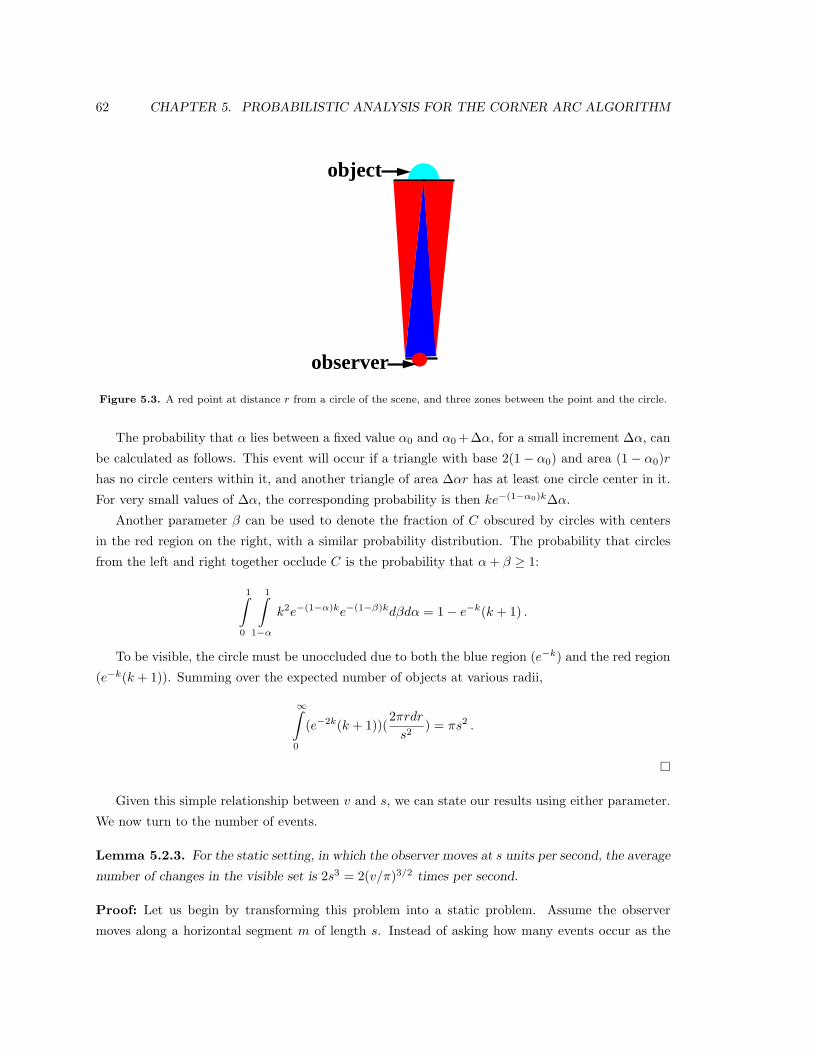
62 CHAPTER 5. PROBABILISTIC ANALYSIS FOR THE CORNER ARC ALGORITHM
object
observer
Figure 5.3. A red point at distance r from a circle of the scene, and three zones between the point and the circle.
The probability that α lies between a fixed value α0 and α0 +∆α, for a small increment ∆α, can
be calculated as follows. This event will occur if a triangle with base 2(1− α0) and area (1 − α0)r
has no circle centers within it, and another triangle of area ∆αr has at least one circle center in it.
For very small values of ∆α, the corresponding probability is then ke−(1−α0)k∆α.
Another parameter β can be used to denote the fraction of C obscured by circles with centers
in the red region on the right, with a similar probability distribution. The probability that circles
from the left and right together occlude C is the probability that α + β ≥ 1:
1∫
0
1∫
1−α
k2e−(1−α)ke−(1−β)kdβdα = 1− e−k(k + 1) .
To be visible, the circle must be unoccluded due to both the blue region (e−k) and the red region
(e−k(k + 1)). Summing over the expected number of objects at various radii,
∞∫
0
(e−2k(k + 1))(2πrdr
s2) = πs2 .
¤
Given this simple relationship between v and s, we can state our results using either parameter.
We now turn to the number of events.
Lemma 5.2.3. For the static setting, in which the observer moves at s units per second, the average
number of changes in the visible set is 2s3 = 2(v/π)3/2 times per second.
Proof: Let us begin by transforming this problem into a static problem. Assume the observer
moves along a horizontal segment m of length s. Instead of asking how many events occur as the
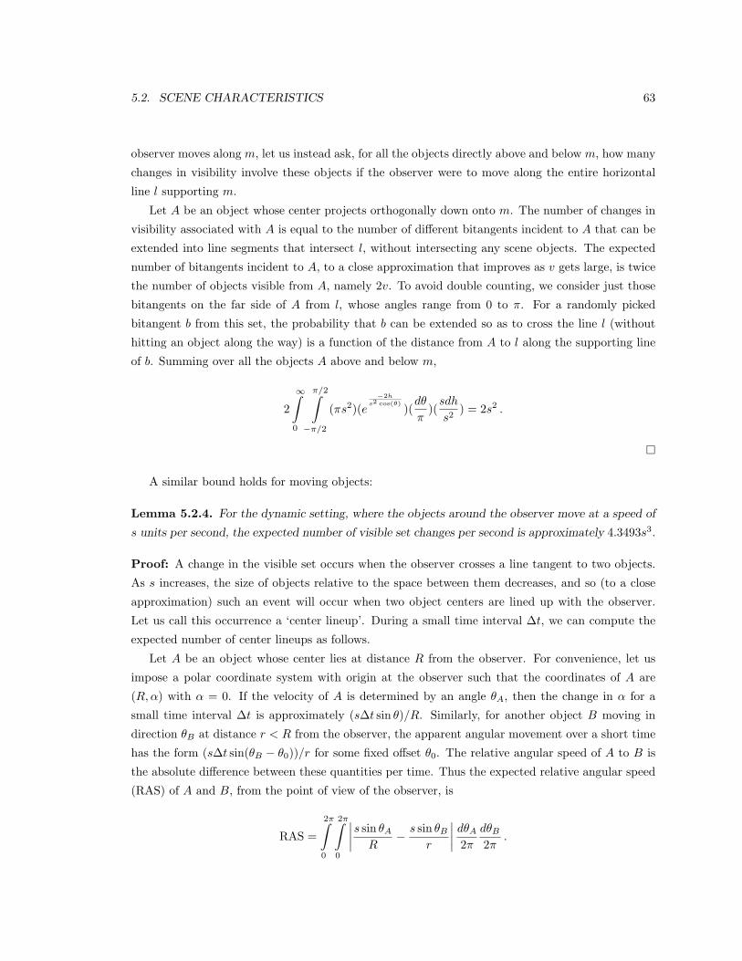
5.2. SCENE CHARACTERISTICS 63
observer moves along m, let us instead ask, for all the objects directly above and below m, how many
changes in visibility involve these objects if the observer were to move along the entire horizontal
line l supporting m.
Let A be an object whose center projects orthogonally down onto m. The number of changes in
visibility associated with A is equal to the number of different bitangents incident to A that can be
extended into line segments that intersect l, without intersecting any scene objects. The expected
number of bitangents incident to A, to a close approximation that improves as v gets large, is twice
the number of objects visible from A, namely 2v. To avoid double counting, we consider just those
bitangents on the far side of A from l, whose angles range from 0 to π. For a randomly picked
bitangent b from this set, the probability that b can be extended so as to cross the line l (without
hitting an object along the way) is a function of the distance from A to l along the supporting line
of b. Summing over all the objects A above and below m,
2
∞∫
0
π/2∫
−π/2
(πs2)(e−2h
s2 cos(θ))(
dθ
π)(
sdh
s2) = 2s2 .
¤
A similar bound holds for moving objects:
Lemma 5.2.4. For the dynamic setting, where the objects around the observer move at a speed of
s units per second, the expected number of visible set changes per second is approximately 4.3493s3.
Proof: A change in the visible set occurs when the observer crosses a line tangent to two objects.
As s increases, the size of objects relative to the space between them decreases, and so (to a close
approximation) such an event will occur when two object centers are lined up with the observer.
Let us call this occurrence a ‘center lineup’. During a small time interval ∆t, we can compute the
expected number of center lineups as follows.
Let A be an object whose center lies at distance R from the observer. For convenience, let us
impose a polar coordinate system with origin at the observer such that the coordinates of A are
(R, α) with α = 0. If the velocity of A is determined by an angle θA, then the change in α for a
small time interval ∆t is approximately (s∆t sin θ)/R. Similarly, for another object B moving in
direction θB at distance r < R from the observer, the apparent angular movement over a short time
has the form (s∆t sin(θB − θ0))/r for some fixed offset θ0. The relative angular speed of A to B is
the absolute difference between these quantities per time. Thus the expected relative angular speed
(RAS) of A and B, from the point of view of the observer, is
RAS =
2π∫
0
2π∫
0
∣∣∣∣s sin θA
R− s sin θB
r
∣∣∣∣dθA
2π
dθB
2π.

64 CHAPTER 5. PROBABILISTIC ANALYSIS FOR THE CORNER ARC ALGORITHM
Given the relative angular speed of movement, the probability of having a center lineup between
A and B is ∆tRAS/2π. This probability can then be summed over all objects B at distances less
then R from the observer to obtain the expected number of center lineups (CL) that have to do with
A as the farther object:
CL =
R∫
0
(∆tRAS
2π)(
2πrdr
s2)
=∆t
s(
12π
)2R
1∫
0
2π∫
0
2π∫
0
|ρ sin θA − sin θB |dθAdθBdρ
≈ 27.3277∆t
s(
12π
)2R
Finally the probability of having a change in visibility with A as the farther object is four times
the number of center line-ups (one for each possible line tangent to two objects) times the probability
of having a clear line of sight from the observer to A: 4CLe−2R/s2. The expected number of events
per second is then:
∞∫
0
4(27.3277∆t
s(
12π
)2R)e−2R/s2 2πRdR
s2≈ 4.3493s3 .
¤
Thus the number of visibility events for both the static and moving scenes are asymptotically
the same up to a constant factor, if the motion in both cases is of the same speed and the objects
are spread out to the same extent.
5.3 Corner Arc Algorithm Complexity
The complexity of the corner arc algorithm depends on both the number and cost of the various
kinetic updates. In the average case setting presented here, we assume event times can be modeled
as arising from a known random distribution. Therefore the expected cost of changes to the event
heap will be constant when bucketing techniques are used. Most of the kinetic updates, such the
pseudo-triangle updates, require only constant time each. The visibility updates, on the other hand,
may involve many pseudo-triangle flips. The first step in analyzing the complexity of the corner arc
algorithm is to compute the expected cost (over many updates) of a single tangency event.

5.3. CORNER ARC ALGORITHM COMPLEXITY 65
5.3.1 Cost of Tangency Events
To compute the expected average number of flips for a tangency event, one approach would be to
examine the local combinatorial structure in the neighborhood of such an update, as is typically
done in worst-case analysis. However, the behavior of the corner arc algorithm is history dependent:
The number of flips at one event depends on the number of flips at a previous event, and so on,
until the configuration of bitangents becomes difficult or impossible to predict. Another approach
is therefore needed to bound the complexity.
Although the position of bitangents in the pseudo-triangulation overall is history-dependent,
there are some bitangents whose positions do not depend on the prior motion, namely the bitangents
that lie along corner arcs. One approach, then, to characterizing the complexity of the corner arc
algorithm is to develop statistical descriptions of the behavior of the bitangents that fall along corner
arcs, and use this information to bound the behavior of the other bitangents.
To be more precise, let us divide the bitangents of the pseudo-triangulation into two groups,
the “arc” and “non-arc” bitangents. Initially, all bitangents are considered non-arc bitangents.
Whenever a bitangent is flipped, if in being flipped it becomes part of a corner arc, then it is called
an arc bitangent. Otherwise, it is called a non-arc bitangent. That is, a bitangent b is considered
an arc bitangent if, at the last time b was flipped, b landed on a corner arc. Otherwise, b is a non-arc
bitangent. The arc bitangents and the non-arc bitangents may be modified by pseudo-triangle event
updates, but such modifications do not affect the division into arc and non-arc bitangents.
To characterize the costs associated with tangency events, let us begin by exploring characteristics
associated with arc bitangents.
Lemma 5.3.1. The expected average number of bitangents along a corner arc is between 1.189 and
1.25, regardless of the spacing s.
Proof: The number of bitangents along a corner arc is one more than the number of intermediate
objects along the corner arc, not counting the tangent and far objects of the boundary segment.
Any intermediate object must overlap a triangle formed by the boundary segment and part of the
far object. If this triangle has area A, then the number of intermediate objects within it is no more
than the expected number of overlapping objects: A/s2. On the other hand, if there is at least one
overlapping object (with probability 1− e−A/s2), then the number of intermediate objects must be
at least one. To compute the area A, the height of the triangle is uniformly distributed between
0 and 2, and the base length is distributed according to the probability of having a clear line of
sight to distance r followed by an object within a small additional distance ∆r of e−2r/s2( 2∆r
s2 ). The
desired upper and lower bounds are thus:
∫ 2
0
∫ ∞
0
(1 +rh
2s2)e−2r/s2 2dr
s2
dh
2= 5/4 .
and

66 CHAPTER 5. PROBABILISTIC ANALYSIS FOR THE CORNER ARC ALGORITHM
∫ 2
0
∫ ∞
0
(1e−rh/2s2+ 2(1− e−rh/2s2
))e−2r/s2 2dr
s2
dh
2= 2(1 + log 2/3) ≈ 1.189 .
¤
Because the expected number of bitangents along a corner arc is constant, the cost of marking
the bitangents along corner arcs will also be constant if the marking approach is used for handling
reflex events. We will assume marking is used to simplify the later analysis of pseudo-triangle events.
We next bound the number of arc bitangents at a given radius from the observer. To obtain a
lower bound for this population, one approach would be to lower bound the expected number of arc
bitangents that are created per second, and lower bound the expected time each such arc remains
untouched by further visibility events (i.e. the expected average time between flips, for a typical
arc bitangent), and put these estimates together. The latter quantity, namely the expected average
time between flips, can be calculated as follows.
The probability that a given arc bitangent b will be flipped during a given short time interval ∆t
depends on the position of b. If b is near the observer where many visibility events are occurring,
then the chances of being flipped are higher, but if the endpoints of the bitangent span a very small
sector of the field of view of the observer, then the chances are reduced. The first task, then, in
analyzing the expectation of flipping an arc bitangent is to characterize its position, and the change
in its position over time. The distance of an arc bitangent from the observer is initially dependent
on the distances of changes in visibility from the observer, and this distribution was calculated
already for the sake of counting the expected number of changes in visibility during a given time
interval. Over time, a bitangent may move toward or away from the observer, but it will be shown
that a bitangent cannot move significantly closer or farther from the observer in the typical interval
between flips.
As long as an arc bitangent b is part of a corner arc, it will be very nearly aligned with the
observer, since for large s the average length of a boundary segment is large in comparison with
the width of a far object (the expected average length is s2/2). Over time, however, the objects to
which a bitangent is connected may move apart. The width of a bitangent is the sector of the field
of view of the observer covered by a bitangent, measured in radians. To a close approximation, the
width begins at zero, and increases with the expected separation of the objects to which it connects.
More precisely,
Lemma 5.3.2. The expected increase in width of an arc bitangent b with nearer endpoint at dis-
tance r from the observer over the course of a time period t is upper bounded by cest/r, where
ce ≈ .811.
Proof: Let A and B be the two objects on either end of b. Let r be the distance between the
observer and the closer of A and B. The expected average speed at which A and B separate is

5.3. CORNER ARC ALGORITHM COMPLEXITY 67
greatest when both objects lie at roughly the same distance from the observer. Also, although b
may move off of A and/or B due to pseudo-triangle events, the expected speed of separation of any
such new objects will not be more than the expected speed of separation of A and B. It thus suffices
to consider the relative speed of two points moving on a circle of radius r:
2π∫
0
2π∫
0
∣∣∣∣st sin θ1
r− st sin θ2
r
∣∣∣∣dθ1
2π
dθ2
2π≈ 0.811st
r.
¤
A simple model of the position and movement of an arc bitangent b over time is then as follows:
Let r be the distance from the observer to the near endpoint of b when b is first flipped. Let a be
an arc of the circle of radius r around the observer with central angle cest/r, at time t. Thus the
width of the arc is expected to be greater than that of b, at a similar distance from the observer, as
time progresses. The probability that b will be flipped during a short time interval t is thus upper
bounded by the probability that a boundary segment will cross a during the same time interval.
This latter probability has two components: either a boundary segment will gradually move across
one of the endpoints of a, or a boundary segment will suddenly appear through the middle of a due
to a visibility event. (The probability that a boundary segment will move through the middle of a
due to object movement is negligible in comparison to these factors for small arcs.) To bound these
two components, we first bound the number of times an object center passes underneath an endpoint
of a, and the number of times two object centers align beneath a, using the same calculation as used
earlier in deriving the number of changes in visibility:
Lemma 5.3.3. The number of object centers passing beneath an endpoint of arc a is C1 = µtr/4πs,
and the number of center alignments below a is C2 = ceµr2t2/48πs2 where µ ≈ 17.3973.
We are now ready to estimate the time between flips for an arc bitangent b. At a high level, this
is just a matter of integrating the probability that none of the passages and alignments C1 and C2
occur when no other objects block a line of sight from the observer to a. However, since this bound
will be used in later derivations, it will be important to have a simple form of it, which is still a
lower bound.
Lemma 5.3.4. The expected average time between the creation and destruction of an arc bitangent
b whose near endpoint begins at distance r from the observer is at least L1(r) = 1/s when 0 ≤ r ≤2.6s2, and at least L2(r) = 1.022(s/r)er/s2
when r ≥ 2.6s2.
Proof: The probability that a single one of the passages and alignments C1 and C2 occurs at a time
that another object blocks the view of the observer to see all the way to arc a along the implied line
is x = 1 − e−2r/s2, and the probability that none of these events occur is xC1+C2 . The probability
68 CHAPTER 5. PROBABILISTIC ANALYSIS FOR THE CORNER ARC ALGORITHM
that the destruction of b happens before time t is then at most 1− xC1+C2 , and the expected time
until this flip is at least
∞∫
0
t(d
dt(1− xC1+C2))dt .
Unfortunately, this integral seems difficult to evaluate symbolically, due to the differing powers
of t in the exponent of x. C1 > C2 from t = 0 to t = 12s/cer, after which C2 > C1. An upper bound
can be obtained by replacing the sum C1 + C2 by 2C1 and 2C2 for the appropriate time intervals.
The result of the integral is then as follows:
12s/cer∫
0
t(d
dt(1− x2C1))dt +
∞∫
12s/cer
t(d
dt(1− x2C2))dt =
s
r(T1 + T2)
where
T1 =2π(x6µ/ceπ − 1)
µ log x
and
T2 =
√6π(1− Erf[
√6µceπ
√− log x])√
ceµ√− log x
.
By inspection of a numerically generated graph, the first term, sr T1, is greater than 1/s when
0 ≤ r ≤ 2.6s2. The second term sr T2 increases monotonically with r, beginning at zero. In the
second term, when r ≥ 2.6s2, the error function Erf[] value is between zero and one half. For these
values of r, a lower bound to T2 is thus
T3 =12
√6π√
ceµ√− log x
.
Let y = e−2r/s2, so that x = 1− y. Since r ≥ 2.6s2 implies y ≤ e−5.2, then
1√− log x=
1√y(− 1
y log(1− y))
≥ 1√y(− 1
e−5.2 log(1− e−5.2))
≈ 0.9981√y

5.3. CORNER ARC ALGORITHM COMPLEXITY 69
and thus a lower bound on T3 for r ≥ 2.6s2 is
0.998√
3π√2ceµ
er/s2 ≈ 1.022er/s2.
¤
We can now use these bounds to compute a bound on the expected number of flips per visibility
event:
Theorem 5.3.5. The expected average number of flips per visibility event in the corner arc algo-
rithm is no more than 19.046 for the randomly generated scenes of moving objects described above,
regardless of the spacing s.
Proof: The overall strategy for bounding the number of flips is to examine the population of arc
bitangents at various distances from the observer. Except possibly for distances r very near the
observer, in general the proportion of arc bitangents among all bitangents at a distance r decreases
as r increases. Thus for a conservative bound, it is better to overestimate than underestimate the
distance from the near endpoint of a bitangent to the observer.
A visibility event occurs when at least one boundary segment becomes tangent to two objects
simultaneously. Suppose for a particular event the two objects lie at distances r1 and r2 from the
observer, where r1 > r2. The distance to the near endpoint of the bitangent or bitangents created
along the new corner arc(s) will be typically be between r1 and r2, though sometimes (in the case
of shaft events) a new arc bitangent could conceivably have its near endpoint at a distance greater
than r2. The distance from the observer to this visibility event will be defined as the larger of r1
and r2.
Let α(r) represent the expected average number of arc bitangents created per visibility event at
distance r from the observer. Let nvis(r) = µ(r2/s3)e−2r/s2∆r be the expected average number of
visibility events per second in a small annulus at distance r from the observer of width ∆r. The ex-
pected average number of arc bitangents whose near endpoints lie in this annulus at a given moment
is lower bounded by the expected average number of arc bitangents created per second times the
expected average number of seconds between the creation and destruction of a single arc bitangent:
α(r)nvis(r)L(r). The expected number of bitangents inside this annulus is three times the number
of objects with centers inside the annulus: nbitangent(r) = 3(2πr/s2)∆r. Putting these together,
the ratio of all bitangents to arc bitangents in this annulus is then upper bounded by ratio(r) =
nbitangent(r)/(α(r)nvis(r)L(r)). Assuming that this ratio is the same for the general population of bi-
tangents as for the bitangents encountered during the flips involved in visibility events, the expected
average number of flips per visibility event is nflips(r) = α(r)ratio(r) = nbitangent(r)/(nvis(r)L(r)).
In other words, it is not necessary to estimate α(r) to obtain a bound on the number of flips per
event.

70 CHAPTER 5. PROBABILISTIC ANALYSIS FOR THE CORNER ARC ALGORITHM
Plugging in the specific bounds for the expected average time between flips for arc bitangents,
the expected average number of flips that occur per second at distances less than s2 log s are:
2.6s2∫
0
nflips(r)nvis(r)dr =
2.6s2∫
0
nbitangent(r)/L1(r)dr
=
2.6s2∫
0
(3(2πr/s2))/(1/s)dr
≈ 63.711s3 ,
and
s2 log s∫
2.6s2
nflips(r)nvis(r)dr =
s2 log s∫
2.6s2
nbitangent(r)/L2(r)dr
=
s2 log s∫
2.6s2
(3(2πr/s2))/(1.022(s/r)er/s2)dr
≈ 19.124s3 + o(s3) .
Over the same distances, the number of visibility events are approximately 3.876s3 and 0.473s3+
o(s3), respectively, so the expected average number of flips for all visibility events up to distance
r = s2 log s is at most 19.046. Beyond this distance, the number of events is so few that even if the
average complexity were as high as s flips per event, the number of such flips would not contribute
asymptotically to the total. ¤
The bound on the expected average number of flips per tangency event must be combined with
the cost of individual flips to obtain the expected cost of tangency updates:
Lemma 5.3.6. The expected cost of a flip operation in this setting is O(log s).
Proof: The time complexity of flipping a bitangent b is at most proportional to the number of sides
along the two pseudo-triangles adjacent to b. The average number of sides along a pseudo-triangle
anywhere in the scene is bounded by a constant (the total number of bitangents along pseudo-triangle
sides is less than 6N , and the total number of pseudo-triangles is 2N − 2). However, during the
course of a visibility update, the sequence of flips can create progressively longer pseudo-triangles
that could conceivably have many bitangents along their sides. Although these pseudo-triangles
can be as long as boundary segments, they can only be as wide as the bitangents allow, which is

5.3. CORNER ARC ALGORITHM COMPLEXITY 71
on average O(s). The area within which these pseudo-triangles are formed is at most O(s2s), and
thus the expected number of objects overlapping this area is at most O(s). The expected number
of sides on the convex hull for a uniform distribution of points inside a rectangle is logarithmic in
the number of points, so the expected number of sides along such a pseudo-triangle is bounded by
O(log s). ¤
The cost of individual flips can be reduced further using acceleration structures along the sides of
pseudo-triangles [PV96a] to O(log log s). In practice, however, when the number of objects simulta-
neously visible to an observer is less than 10, 000, the average number of sides along a pseudo-triangle
is less than 5 and thus the simpler O(log s) flip may perform just as well. In conclusion:
Corollary 5.3.7. The expected cost of a tangency event in this setting is O(log s).
5.3.2 Cost of Other Event Types
The remaining cost of the corner arc algorithm is due to event types other than tangency events.
In particular, pseudo-triangle events can be particularly numerous near the observer, while collision
events may have a lesser impact on the total running time. The discussion below addresses collision
events first, then pseudo-triangle events.
The number of collision events per object per second decreases as the spacing s between objects
increases. For a given object A, the probability that A will collide with another object during
one second depends on the likelihood of having two extruded segments in space-time overlap, and
this probability will decrease as the space-time object volumes move apart. Also, if a global scene
bounding box is used, the number of collisions per second with the scene bounding box depends on
the number of objects within a distance s from the scene bounding box, which is asymptotically less
than the total number of objects. Thus the number of collisions grows asymptotically insignificant
in comparison with events whose frequency is proportional to the total number of objects. The cost
of a single collision update is constant, since the number of bitangents connected to a given object
is a constant on average.
The number of pseudo-triangle events per second is at least proportional to the number of
objects in the scene. The cost of pseudo-triangle events far from the observer, or in a scene without
an observer, can be bounded as follows:
Lemma 5.3.8. The expected number of pseudo-triangle events for maintaining a pseudo-triangulation
in a dynamic scene without an observer and a constant speed of motion for each object is O(N)
events per second, regardless of the spacing s between objects.
Proof: Consider two scenes with the same total number of objects N but different spacing between
objects, s1 and s2. Suppose that a coordinate system are chosen where the unit of length is propor-
tional to the spacing between objects, rather than the width of a single object. That is, the spacing

72 CHAPTER 5. PROBABILISTIC ANALYSIS FOR THE CORNER ARC ALGORITHM
between objects is fixed, and it is the size of objects that is varied, rather than the other way around.
Suppose further that the positions of the object centers, in this new coordinate system, is exactly
the same for the two scenes. Also suppose that the velocities of the objects is chosen to be the same
in the two scenes. In this setting, except for the effect of collisions, the number of pseudo-triangle
events in the two scenes will be exactly the same. Thus there is a perfect correspondence between
the space of possible scenes of spacing s1 and spacing s2, with the same number of pseudo-triangle
events, except in the event of a collision. But we have already seen that for large s, the effect of
collision is negligible, so the number of pseudo-triangle events is asymptotically independent of s.
On the other hand, if the size of the scene N is increased, then the number of pseudo-triangle events
will increase as the number of pseudo-triangles, which is linear in N . ¤
If N is chosen to be O(s3), the cost of these events far from the observer will be asymptotically
no more than than the cost of tangency events. However, the number of pseudo-triangle events near
to the observer can be higher:
Lemma 5.3.9. The number of pseudo-triangle events per second that arise due to visibility main-
tenance near the observer is O(s3 log2 s).
Proof: The influence of the construction of corner arcs beyond a distance of 2s2 log s from the
observer is negligible for large s, since the expected number of events beyond that distance is
O(log2 s/s). Within that distance, the total number of objects is 4s2 log2 s. If all the bitangents
were perfectly aligned with the observer, then the pseudo-triangle events would happen as often as
every 1/s seconds per object, since it would take this long for an object to travel a distance equal
to (a constant times) the width of an object. Thus the expected number of pseudo-triangle events
per second that result from the configuration of bitangents near the observer is at most s times the
number of objects within this radius. ¤
The cost of a single pseudo-triangle event update is constant, so the expected cost attributable
to this type of event per second is the same as the expected cost attributed to tangency events, up
to a poly-logarithmic factor.
In conclusion the complexity of the corner arc algorithm for average case dynamic scenes can be
described as follows:
Theorem 5.3.10. The average cost per change in visibility in the dynamic scene, including the
costs of non-visibility related events, is O(log2 s).
The best possible cost of a temporally coherent algorithm of this type is a cost of a constant
amount of computation per change in visibility, so the corner arc algorithm is optimal up to a poly-
logarithmic factor. In addition, we claim that an optimal or near-optimal algorithm also exists for
the simpler problem of maintaining visibility in a static scene, which implies the following:

5.4. CONCLUSION 73
Corollary 5.3.11. The intrinsic complexity of maintaining visibility in a temporally coherent man-
ner for static and dynamic scenes as described above is asymptotically the same, up to a poly-
logarithmic factor in v, the number of visible objects.
5.4 Conclusion
The corner arc algorithm is a relatively simple kinetic algorithm for maintaining visibility from
a point observer among moving objects in the plane, using a pseudo-triangulation for the spatial
subdivision. The size of the data structure is proportional to the number of objects, the size of the
event heap is proportional to the number of moving objects (plus the number of visible objects, if
there are only a few moving objects), and the computation associated with individual updates is local,
in the sense that the only objects affected by events touch the pseudo-triangles in the neighborhood
of the events. This algorithm is optimal up to a poly-logarithmic factor for an average case setting of
moving objects, and thus provides the first non-trivial result on the intrinsic complexity of temporally
coherent visibility maintenance in a dynamic setting.

74 CHAPTER 5. PROBABILISTIC ANALYSIS FOR THE CORNER ARC ALGORITHM
Chapter 6
2D Implementation Results
How fast are 2D visibility maintenance algorithms when implemented on current hardware? The
cost of maintaining visibility with the corner arc algorithm has been estimated probabilistically in
chapter 5 to be nearly proportional to the number of changes in visibility, for an average case scene.
To verify this analysis and examine the constant factors involved, we have implemented the corner
arc algorithm, as well as the visible zone algorithm, and tested these algorithms on scenes with
millions of objects. The results indicate that for the corner arc algorithm, the cost of visibility
maintenance on an R10000 CPU is approximately 100,000 clock cycles per change in visibility in
the static case (where only the observer moves), and approximately a million cycles per change in
visibility when all the objects of the scene are in motion.
This chapter is organized in three sections as follows: 1) a description of how the test scenes
were generated and the motion of the objects, 2) characteristics of these test scenes relevant to
any visibility maintenance algorithm, and 3) a comparison of four 2D visibility algorithms, with a
detailed description of the performance of the corner arc algorithm.
6.1 An Average Case Setting
Although many insights into the behavior of algorithms generally may be obtained from study of
worst case inputs, the type of visibility algorithms that predominate in practice derive their efficiency
from taking advantage of the coherence found in typical inputs. Quantifying what a typical scene
is remains a challenge, although many popular visibility algorithms are most obviously suited to
either a uniform distribution of objects or perhaps a uniform distribution of uniform distributions,
as implied by the popularity of multi-grid ray-tracing techniques.
We have chosen to test these kinetic visibility algorithms on randomly generated scenes consisting
of N unit circles distributed uniformly in a rectangle of the plane, with the observer in the center
of the rectangle. The unit circles are represented using regular octagons of perimeter 2π. The
75

76 CHAPTER 6. 2D IMPLEMENTATION RESULTS
direction of motion of any moving object is also chosen uniformly at random. Although these results
are computed in the plane, with the techniques to be presented in chapter 7 this analysis may be
seen as a component of the complexity of a 3D algorithm.
The difficulty of computing visibility is often related to the expected number of objects v visible
to the observer: as v increases, the expected number of changes in visibility that must be processed
for a small movement of the observer may increase as well. Also, as v increases, it may be necessary
to search further to find the objects involved in changes in visibility, because the scene is more sparse.
The size of the visibility complex increases linearly with v, given a fixed number of objects N in the
scene. As another example of the impact of increasing the number of visible objects, shooting a ray
through a grid has a cost proportional to the number of grid cells intersected, which increases as√
v
(in the uniformly distributed context that is assumed). We explore the performance of the corner
arc algorithm as the number of visible objects v increases.
While the parameter v captures the sparsity of the scene from the point of view of the observer,
the sparsity of the scene can also be described by the parameter s, which is the side length of a
square whose expected occupancy is one. In some cases, such as in describing distances, s may be a
more intuitive measure since it approximates the average distance between two neighboring objects.
In order to avoid boundary effects in the performance of the corner arc algorithm on scenes with
different numbers of visible objects, the total number N of objects and the area of the rectangle
in the plane containing the scene is chosen large enough that the observer cannot see through the
objects to the boundary of the scene. More specifically, since the number of visible objects beyond
a distance of s2 log s goes asymptotically to zero as s increases, the test scenes are constructed so
that the nearest boundary of the scene is at a distance of at least 7s2 log s from the observer, which
means that the total number objects N is greater than 49s2 log2 s. In practice, this means that to
generate results where the observer can see 5,000 objects at once, the total number N of objects in
the scene is roughly one million.
The difference between the cost of maintaining visibility in a scene with static objects and a scene
with moving objects has not been systematically described before. We compare two possibilities for
the motion in the scene: 1) in the ‘static’ setting, the objects do not move and the observer moves
along a linear trajectory free of obstacles, and 2) in the ‘dynamic’ setting, the observer does not
move but all the objects of the scene are given linear trajectories. In both cases, the speed of motion
is chosen to be s units per second of simulation time (not CPU time).
6.2 Visibility-Related Characteristics
The expected number of visible objects v is not necessarily the same as the actual number of visible
objects for a given observer position in a given randomly generated scene. Given v, the test scenes
are actually generated by setting values for N and s which correspond to the chosen value of v

6.2. VISIBILITY-RELATED CHARACTERISTICS 77
according to the probability analysis. Figure 6.1 compares the expected to the actual number of
visible objects in the test scenes. For each value of v that we tested, approximately 100 simulations
were run and the actual number of visible objects was recorded at several times during each run.
The average over all runs, as well as the standard deviation across runs, is indicated in red. This
data follows the line of slope one, as expected.
100
1000
10000
100 1000 10000
actu
al n
umbe
r of
vis
ible
obj
ects
expected number of visible objects v
Figure 6.1. The expected number of visible objects v compared with the actual number of visible objects for a seriesof experiments. The averages and standard deviations are shown in red, and the line of slope 1 is shown in green.
The probabilistic analysis indicates that v = πs2 on average, so the number of visible objects
increases much more quickly than the typical inter-object spacing. The number of changes in the
visible set per second is predicted to be proportional to s3, as verified in Figure 6.2.
0
1
2
3
4
5
6
100 1000 10000
visi
bilit
y ev
ents
div
ided
by
s3
expected number of visible objects v
Figure 6.2. The number of changes in visibility per second divided by s3 is shown in red, and appears to be roughlyconstant. The expected constant of proportionality is shown as a green line.
As the number of visible objects increases, the number of visibility events goes up roughly as the
product vs, for both the static and moving scenes. Thus the increase in the number of events as the

78 CHAPTER 6. 2D IMPLEMENTATION RESULTS
scene becomes more sparse is somewhat super-linear in v, but not quadratic.
The behavior of static scenes and moving scenes are similar with regard to both the number
of visible objects and the number of changes in visibility per second under the motion described
above. However, there are several differences between the two settings. One such difference is in
the number of collisions. For the sake of simplicity, we construct the static scene in such a way
that the observer will never collide with any scene object, thus introducing a slightly non-uniform
distribution of objects near the observer’s trajectory.
The number of collisions in the moving scene depends on N , the total number of objects, as well
as v. If v is held fixed, the dependence on N is linear for ordinary collisions, and sub-linear for
collisions with a global scene boundary (see Figure 6.3).
0
0.02
0.04
0.06
0.08
0.1
0.12
0.14
0.16
0.18
1000 10000 100000
colli
sion
s (b
oth
type
s) p
er o
bjec
t per
sec
ond
number of objects N
Figure 6.3. The average number of two-object collisions per object per second (red) remains steady as the numberof objects increases, and the number of collisions with the boundary (green) decreases (at v = 1000).
However, if N is held fixed, and v is varied (see Figure 6.4), the number of collisions per object
decreases with increasing v. Thus as long as the total number N of objects in the scene increases
more slowly than the number of changes in visibility, the asymptotic costs of handling changes in
visibility will dominate the cost of handling collision events.
An implication of this characterization of the number of collision events with the scene boundary
is that if we classify the objects of the scene into two sets – those that are found in a reasonable
proximity of the observer and those far away – then the transitions between these two sets are
relatively rare, as compared to the number of changes in the visible set. Although we do not explore
this fact here, it implies that significantly larger scenes could possibly be accommodated with such
a two-set approach.
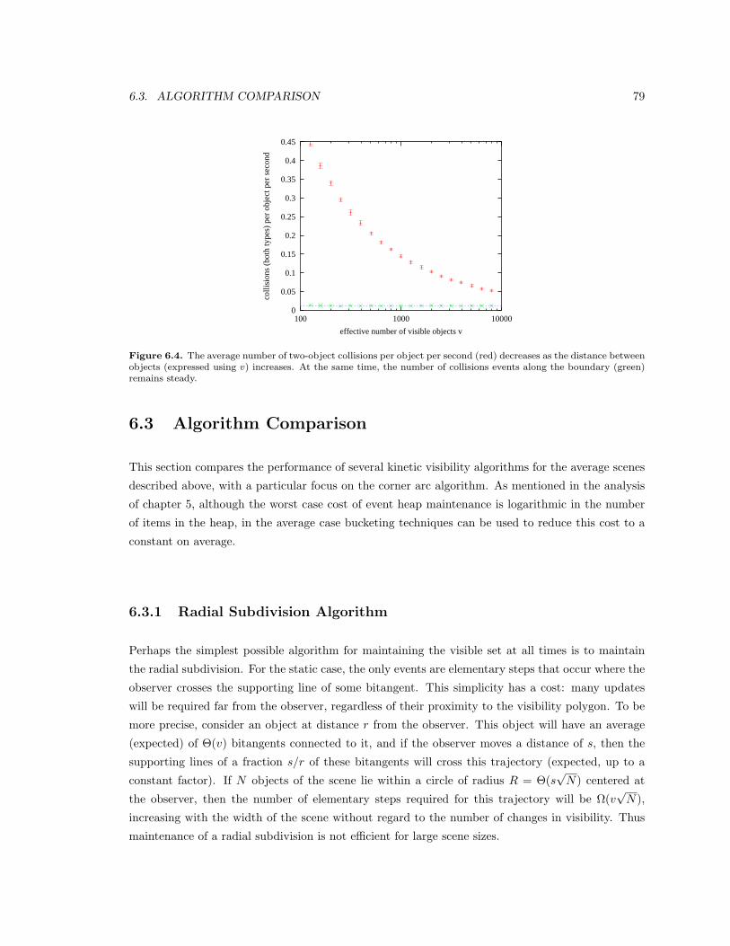
6.3. ALGORITHM COMPARISON 79
0
0.05
0.1
0.15
0.2
0.25
0.3
0.35
0.4
0.45
100 1000 10000
colli
sion
s (b
oth
type
s) p
er o
bjec
t per
sec
ond
effective number of visible objects v
Figure 6.4. The average number of two-object collisions per object per second (red) decreases as the distance betweenobjects (expressed using v) increases. At the same time, the number of collisions events along the boundary (green)remains steady.
6.3 Algorithm Comparison
This section compares the performance of several kinetic visibility algorithms for the average scenes
described above, with a particular focus on the corner arc algorithm. As mentioned in the analysis
of chapter 5, although the worst case cost of event heap maintenance is logarithmic in the number
of items in the heap, in the average case bucketing techniques can be used to reduce this cost to a
constant on average.
6.3.1 Radial Subdivision Algorithm
Perhaps the simplest possible algorithm for maintaining the visible set at all times is to maintain
the radial subdivision. For the static case, the only events are elementary steps that occur where the
observer crosses the supporting line of some bitangent. This simplicity has a cost: many updates
will be required far from the observer, regardless of their proximity to the visibility polygon. To be
more precise, consider an object at distance r from the observer. This object will have an average
(expected) of Θ(v) bitangents connected to it, and if the observer moves a distance of s, then the
supporting lines of a fraction s/r of these bitangents will cross this trajectory (expected, up to a
constant factor). If N objects of the scene lie within a circle of radius R = Θ(s√
N) centered at
the observer, then the number of elementary steps required for this trajectory will be Ω(v√
N),
increasing with the width of the scene without regard to the number of changes in visibility. Thus
maintenance of a radial subdivision is not efficient for large scene sizes.
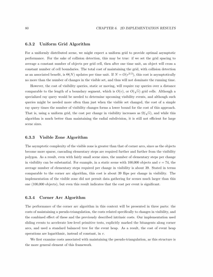
80 CHAPTER 6. 2D IMPLEMENTATION RESULTS
6.3.2 Uniform Grid Algorithm
For a uniformly distributed scene, we might expect a uniform grid to provide optimal asymptotic
performance. For the sake of collision detection, this may be true: if we set the grid spacing to
average a constant number of objects per grid cell, then after one time unit, an object will cross a
constant number of cell boundaries. The total cost of maintaining the grid, with collision detection
as an associated benefit, is Θ(N) updates per time unit. If N = O(v3/2), this cost is asymptotically
no more than the number of changes in the visible set, and thus will not dominate the running time.
However, the cost of visibility queries, static or moving, will require ray queries over a distance
comparable to the length of a boundary segment, which is O(v), or O(√
v) grid cells. Although a
specialized ray query would be needed to determine upcoming visibility events, and although such
queries might be needed more often than just when the visible set changed, the cost of a simple
ray query times the number of visibility changes forms a lower bound for the cost of this approach.
That is, using a uniform grid, the cost per change in visibility increases as Ω(√
v), and while this
algorithm is much better than maintaining the radial subdivision, it is still not efficient for large
scene sizes.
6.3.3 Visible Zone Algorithm
The asymptotic complexity of the visible zone is greater than that of corner arcs, since as the objects
become more sparse, cascading elementary steps are required further and further from the visibility
polygon. As a result, even with fairly small scene sizes, the number of elementary steps per change
in visibility can be substantial. For example, in a static scene with 100,000 objects and v = 74, the
average number of elementary steps required per change in visibility is about 39. Stated in terms
comparable to the corner arc algorithm, this cost is about 39 flips per change in visibility. The
implementation of the visible zone did not permit data gathering for scenes much larger than this
one (100,000 objects), but even this result indicates that the cost per event is significant.
6.3.4 Corner Arc Algorithm
The performance of the corner arc algorithm in this context will be presented in three parts: the
costs of maintaining a pseudo-triangulation, the costs related specifically to changes in visibility, and
the combined effect of these and the previously described intrinsic costs. Our implementation used
sliding events to accelerate low-level primitive tests, explicitly marked the bitangents along corner
arcs, and used a standard balanced tree for the event heap. As a result, the cost of event heap
operations are logarithmic, instead of constant, in v.
We first examine costs associated with maintaining the pseudo-triangulation, as this structure is
the more general element of this framework.
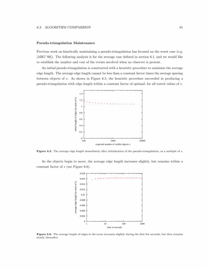
6.3. ALGORITHM COMPARISON 81
Pseudo-triangulation Maintenance
Previous work on kinetically maintaining a pseudo-triangulation has focused on the worst case (e.g.
[ABG+00]). The following analysis is for the average case defined in section 6.1, and we would like
to establish the number and cost of the events involved when no observer is present.
An initial pseudo-triangulation is constructed with a heuristic procedure to minimize the average
edge length. The average edge length cannot be less than a constant factor times the average spacing
between objects of s. As shown in Figure 6.5, the heuristic procedure succeeded in producing a
pseudo-triangulation with edge length within a constant factor of optimal, for all tested values of v.
0
0.2
0.4
0.6
0.8
1
1.2
1.4
100 1000 10000
initi
al le
ngth
of
edge
s (i
n un
its o
f s)
expected number of visible objects v
Figure 6.5. The average edge length immediately after initialization of the pseudo-triangulation, as a multiple of s.
As the objects begin to move, the average edge length increases slightly, but remains within a
constant factor of s (see Figure 6.6).
0
0.002
0.004
0.006
0.008
0.01
0.012
0.014
0.016
0.018
1 10 100 1000
aver
age
edge
leng
th (
in u
nits
of
s)
time in seconds
Figure 6.6. The average length of edges in the scene increases slightly during the first few seconds, but then remainssteady thereafter.

82 CHAPTER 6. 2D IMPLEMENTATION RESULTS
With a constant edge length that is near s, we can expect an object to encounter a constant
number of edges as it moves a distance of s units per second, and the number of pseudo-triangle
events per second should be proportional to the number of moving objects. The number of sliding
events should also be proportional to the number of moving objects. This proportionality for both
pseudo-triangle and sliding events is relatively insensitive to the spacing expressed as a multiple of
v (see Figures 6.7 and 6.8).
0
0.5
1
1.5
2
2.5
3
3.5
4
1000 10000 100000pseu
do-t
rian
gle
and
slid
ing
even
ts p
er o
bjec
t per
sec
ond
number of objects N
Figure 6.7. The average number of pseudo-triangle events (red) and sliding events (green) per object per secondremains steady as the number of objects increases.
0
0.5
1
1.5
2
2.5
3
3.5
4
100 1000 10000pseu
do-t
rian
gle
and
slid
ing
even
ts p
er o
bjec
t per
sec
ond
effective number of visible objects v
Figure 6.8. For a fixed number of objects (N = 10, 000) the average number of pseudo-triangle events per objectper second (red) remains steady as the distance between objects (expressed using v) increases. At the same time, thenumber of sliding events (green) decreases slowly, as the influence of the reflective scene boundary declines.
In summary, the cost of maintaining a pseudo-triangulation for the sake of collision detection is
asymptotically the same in this setting as the cost of maintaining object positions in a uniform grid.

6.3. ALGORITHM COMPARISON 83
Tangency Events
The probabilistic analysis of chapter 5 provided a means of characterizing the complexity of typical
tangency events in terms of a certain population ratio, namely between ‘arc’ edges and ‘non-arc’
edges. This section begins by verifying key elements of that analysis, and then presents overall
statistics on the costs of tangency events.
The definition of arc and non-arc edges is as follows. A tangency event consists in part of flipping
edges. Some of these edges immediately become part of a corner arc as a result of the flip and are
called arc edges, while others do not immediately form part of a corner arc and are called non-arc
edges. This categorization into arc and non-arc persists until the edge is flipped again. Any edges
that have never been flipped are considered non-arc edges. An arc edge is thus ‘created’ when it
is flipped onto a corner arc and ‘destroyed’ when it is flipped again (though it may become an arc
edge, once again).
The rate of creation of arc edges is a function of the number of tangency events, which can in
turn be characterized in terms of the distance from the observer. Figure 6.9 depicts this relationship
for a particular size of scene (v = 1000). The distance from the observer is given as a multiple of s2,
and the green curve indicates the expected average computed in the probabilistic analysis.
0
200
400
600
800
1000
1200
1400
1600
0 1 2 3 4 5
tang
ency
eve
nts
per
seco
nd
distance from observer (in units of s2)
Figure 6.9. The number of tangency events per second as a function of distance from the observer (at v = 1000),compared to the expected average at those distances.
To infer the number of arc edges that will accumulate at a given radius, we also need to know
the average ‘age’ of an arc edge, namely the number of seconds since it was created. Figure 6.10
depicts this quantity, as well as the lower bound derived in the probabilistic analysis.
As the distance to the observer increases, the rate at which arc edges are created goes down, but
the average age of arc edges goes up. Taken together, these factors imply a certain population of arc
edges at any distance from the observer in the steady state. Figure 6.11 depicts the population ratio
(in red) of the total number of (arc or non-arc) edges per arc edge, on average, at various distances
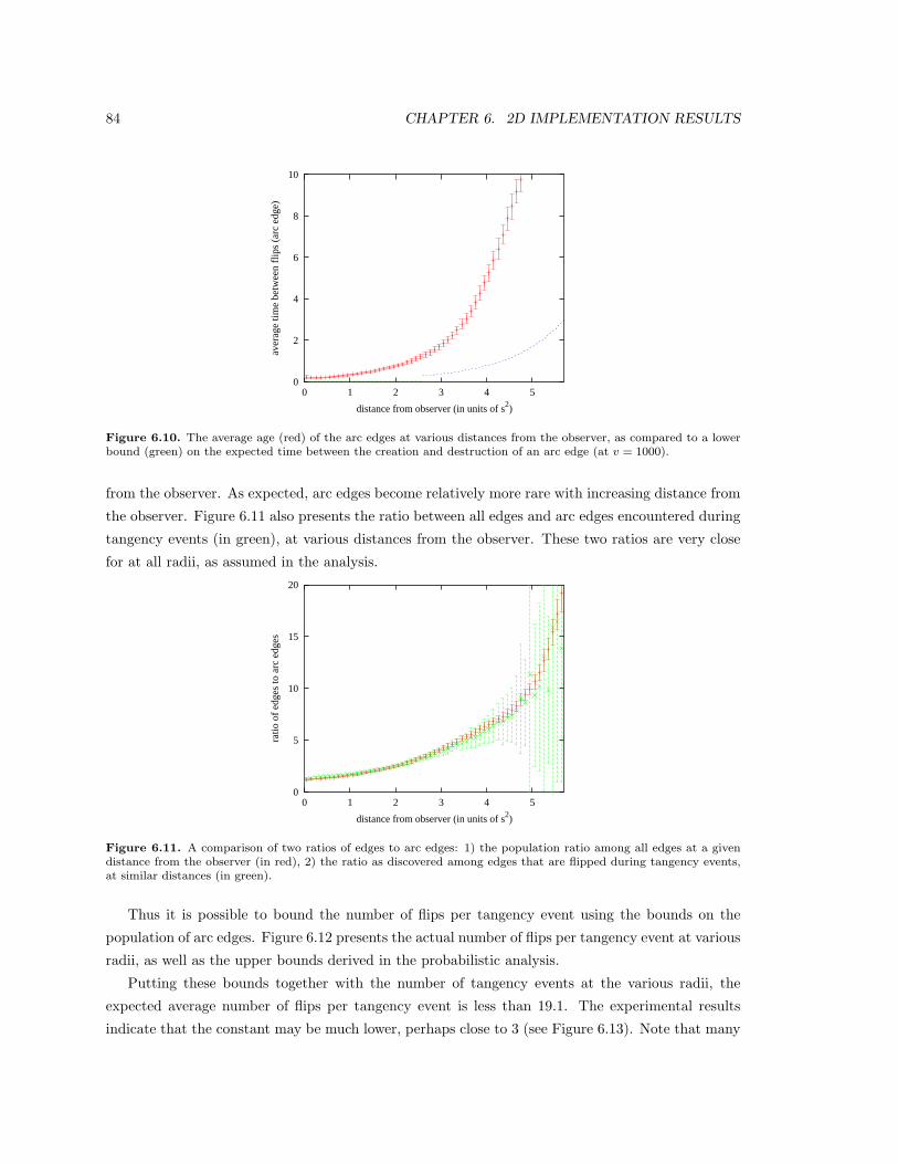
84 CHAPTER 6. 2D IMPLEMENTATION RESULTS
0
2
4
6
8
10
0 1 2 3 4 5
aver
age
time
betw
een
flip
s (a
rc e
dge)
distance from observer (in units of s2)
Figure 6.10. The average age (red) of the arc edges at various distances from the observer, as compared to a lowerbound (green) on the expected time between the creation and destruction of an arc edge (at v = 1000).
from the observer. As expected, arc edges become relatively more rare with increasing distance from
the observer. Figure 6.11 also presents the ratio between all edges and arc edges encountered during
tangency events (in green), at various distances from the observer. These two ratios are very close
for at all radii, as assumed in the analysis.
0
5
10
15
20
0 1 2 3 4 5
ratio
of
edge
s to
arc
edg
es
distance from observer (in units of s2)
Figure 6.11. A comparison of two ratios of edges to arc edges: 1) the population ratio among all edges at a givendistance from the observer (in red), 2) the ratio as discovered among edges that are flipped during tangency events,at similar distances (in green).
Thus it is possible to bound the number of flips per tangency event using the bounds on the
population of arc edges. Figure 6.12 presents the actual number of flips per tangency event at various
radii, as well as the upper bounds derived in the probabilistic analysis.
Putting these bounds together with the number of tangency events at the various radii, the
expected average number of flips per tangency event is less than 19.1. The experimental results
indicate that the constant may be much lower, perhaps close to 3 (see Figure 6.13). Note that many

6.3. ALGORITHM COMPARISON 85
0
5
10
15
20
0 1 2 3 4 5
num
ber
of f
lips
per
angl
e ev
ent
distance from observer (in units of s2)
Figure 6.12. The actual average number of flips per tangency event (red), and the expected upper bounds on thisquantity (green and blue), for various distances from the observer. The frequency of tangency events grows small atlarge distances from the observer, so the available data becomes more sparse.
of these graphs are log-linear, to emphasize the asymptotic behavior as v grows large.
0
0.5
1
1.5
2
2.5
3
3.5
4
100 1000 10000
flip
s pe
r vi
sibi
lity
even
t
expected number of visible objects v
Figure 6.13. The number of flips per tangency event, as a function of the number of visible objects, for a movingscene.
The cost of each such flip is a function of the number of sides along the pseudo-triangles on
each side of flipped edges. The further a tangency event occurs from the observer, the larger
the number of edges that will be flipped, and as a result the number of edges along the sides of
these pseudo-triangles will increase (see Figure 6.14). As a result, the expected overall average
size of pseudo-triangles encountered during these updates may increase with increasing v, with an
estimated bound of O(log v). The actual number of sides along these pseudo-triangles appears to
increase very slowly in practice (see Figure 6.15).
In conclusion, the costs of handling tangency events appears to be nearly constant in practice,
with approximately 3 flips per tangency event and approximately 4 edges per pseudo-triangle next

86 CHAPTER 6. 2D IMPLEMENTATION RESULTS
0
2
4
6
8
10
12
0 1 2 3 4 5
aver
age
edge
s pe
r ps
eudo
-tri
angl
e
distance from observer (in units of s2)
Figure 6.14. The average number edges along triangles encountered during flips, as a function of distance from theobserver (at v = 1000).
0
1
2
3
4
5
6
100 1000 10000
edge
s pe
r ps
eudo
-tri
angl
e
expected number of visible objects v
Figure 6.15. The average number of edges along pseudo-triangles next to flipped edges.

6.3. ALGORITHM COMPARISON 87
to each flipped edge.
Additional Visibility-Related Events
Although the cost of pseudo-triangle events in a scene of moving objects with no observer is pro-
portional to the number of objects, these events may become more numerous when corner arcs are
maintained. One way of examining the influence of corner arc maintenance on the frequency of other
event types is to plot the number of events per object as a function of distance from the observer
(see Figure 6.16). We see that the number of pseudo-triangle events is very much elevated near
the observer, whereas the number of sliding events is actually slightly depressed near the observer.
Thus the sliding events will be no more numerous than in a scene without an observer, but the
pseudo-triangle events may contribute more.
0
5
10
15
20
0 1 2 3 4 5pseu
do-t
rian
gle
and
slid
ing
even
ts p
er o
bjec
t per
sec
ond
distance from observer (in units of s2)
Figure 6.16. The average number of pseudo-triangle (red) and sliding (green) events per object, at various radiifrom the observer, when visibility is maintained.
The increased number of pseudo-triangle events near the observer can be estimated empirically
by taking the total number of pseudo-triangle events, and subtracting the number that would be
expected for a scene that has no observer (see Figure 6.17). It appears that the actual rate of growth
of these events is closer to Θ(s3 log s) than the conservative upper bound of O(s3 log2 s) given by
the probabilistic analysis.
The cost of sliding events associated with maintenance of boundary segments is small in com-
parison to the cost of tangency events, since these sliding events are associated with the rotation of
boundary segments about their tangent objects, which decreases with increasing v.
Total Cost in Moving Scene
The total cost per change in visibility for the corner arc algorithm is the sum of the above mentioned
costs, including collisions, tangency, pseudo-triangle, and sliding events. In the average case setting

88 CHAPTER 6. 2D IMPLEMENTATION RESULTS
0
1
2
3
4
5
6
7
8
100 1000 10000
extr
a cu
sp e
vent
s di
vide
d by
s3 lo
g s
expected number of visible objects v
Figure 6.17. The average number of additional pseudo-triangle events, beyond the events expected when visibilityis not computed, per second as a multiple of s3 log s.
of moving objects described above this cost nearly proportional to the number of changes in visibility,
even when the costs of maintaining all the geometric relationships between non-visible objects are
taken into account (see Figure 6.18). For the scene sizes we tested, the total number of CPU clock
cycles is around one million per change in visibility, even for scenes with a million moving objects.
0
200000
400000
600000
800000
1e+06
1.2e+06
1.4e+06
1.6e+06
1.8e+06
100 1000 10000
CPU
clo
ck c
ycle
s pe
r ch
ange
in v
isib
ility
expected number of visible objects v
Figure 6.18. The average number of CPU clock cycles required to handle each change in visibility on an R10000CPU.
Static Case
The costs of maintaining visibility when the objects are static is predictably lower. There are very
few pseudo-triangle events (only those associated with the movement of the observer, if any) and
similarly few sliding events associated with bitangents. The expected number of changes in visibility,
and thus the number of tangency events, is still proportional to v3/2 (see Figure 6.19). The number
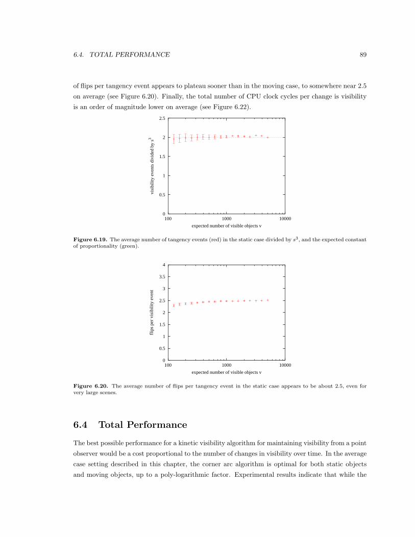
6.4. TOTAL PERFORMANCE 89
of flips per tangency event appears to plateau sooner than in the moving case, to somewhere near 2.5
on average (see Figure 6.20). Finally, the total number of CPU clock cycles per change is visibility
is an order of magnitude lower on average (see Figure 6.22).
0
0.5
1
1.5
2
2.5
100 1000 10000
visi
bilit
y ev
ents
div
ided
by
s3
expected number of visible objects v
Figure 6.19. The average number of tangency events (red) in the static case divided by s3, and the expected constantof proportionality (green).
0
0.5
1
1.5
2
2.5
3
3.5
4
100 1000 10000
flip
s pe
r vi
sibi
lity
even
t
expected number of visible objects v
Figure 6.20. The average number of flips per tangency event in the static case appears to be about 2.5, even forvery large scenes.
6.4 Total Performance
The best possible performance for a kinetic visibility algorithm for maintaining visibility from a point
observer would be a cost proportional to the number of changes in visibility over time. In the average
case setting described in this chapter, the corner arc algorithm is optimal for both static objects
and moving objects, up to a poly-logarithmic factor. Experimental results indicate that while the
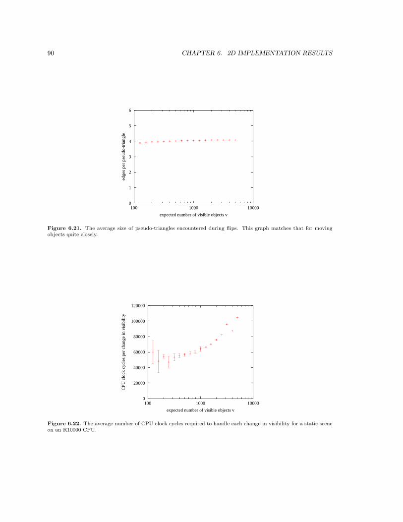
90 CHAPTER 6. 2D IMPLEMENTATION RESULTS
0
1
2
3
4
5
6
100 1000 10000
edge
s pe
r ps
eudo
-tri
angl
e
expected number of visible objects v
Figure 6.21. The average size of pseudo-triangles encountered during flips. This graph matches that for movingobjects quite closely.
0
20000
40000
60000
80000
100000
120000
100 1000 10000
CPU
clo
ck c
ycle
s pe
r ch
ange
in v
isib
ility
expected number of visible objects v
Figure 6.22. The average number of CPU clock cycles required to handle each change in visibility for a static sceneon an R10000 CPU.

6.4. TOTAL PERFORMANCE 91
number of combinatorial updates required for this maintenance involve only small constant factors,
the cost per combinatorial update is nevertheless high in terms of CPU clock cycles.

92 CHAPTER 6. 2D IMPLEMENTATION RESULTS
Chapter 7
Extension to 3D
Most applications of visibility algorithms assume a 3D environment. From the point of view of algo-
rithm design, the difference between 2D and 3D can be dramatic. Temporally coherent algorithms
in particular may be vulnerable to the increase in dimension, since temporal coherence is linked to
ray-space coherence, and the space of rays can be especially complex in 3D.
The intuition for leveraging temporal coherence in 3D is, however, the same as in 2D: as long as
the set of visible objects does not change very much from one frame to the next in an animation, the
cost of maintaining visibility might still compare favorably with the cost of repeatedly rediscovering
all the visible objects.
Previous work on 3D visibility has leveraged temporal coherence to varying degrees. For example,
Coorg and Teller [CT96] first organized a temporally coherent algorithm with an event loop that
processes changes to visibility in time order, whereas later [CT97] they removed the event loop, and
instead periodically updated spatial data structures in such a way that small observer movements
are still relatively efficient.
An approach similar to Coorg and Teller’s can be used to leverage a 2D visibility structure like
the visible zone in 3D. Rather than maintain temporal coherence in the full 3D space, we begin
with a non-temporally coherent, fully 3D algorithm and accelerate low-level queries using the 2D
temporally coherent structure. The result is a robust visibility algorithm for computing visibility
among objects that lie near to a fixed ground plane.
To evaluate the practical utility of this approach, the author and Szymon Rusinkeiwicz have
compared this algorithm with the Occlusion Horizons algorithm of Downs et al. [DMS01] in a real-
time forest fly-though application. The comparison indicates that these two algorithms have similar
computational costs, despite their different organization of the visibility computation.
This chapter is organized as follows. Section 1 discusses some of the difficulties to be surmounted
in designing a temporally coherent algorithm in 3D and briefly describes the non-temporally coherent
method of Downs et al. [DMS01]. Section 2 defines a particular visibility problem that arises in
93
94 CHAPTER 7. EXTENSION TO 3D
practical situations, like navigation of virtual cities. The next three sections describe a partly
temporally coherent algorithm: a fully 3D top-level algorithm, its integration with a visible zone
structure, and approaches to how it can handle more complex objects. Section 6 compares the
performance of these two visibility algorithms, section 7 considers extensions, and section 8 concludes.
7.1 Background
At least three difficulties arise in designing 3D temporally-coherent algorithms.
1. Event time computations may have high constant costs and low accuracy. For example, the
cost of computing a line that passes through four other lines (a vertex of the 3D visibility
complex) may require over 70 multiplications, even when accuracy is not an issue.
2. Update procedures for 3D spatial subdivisions may be complex and prone to robustness prob-
lems, especially when the spatial subdivisions are capable of embedding an approximation to
the visible region.
3. Software-based algorithms must contend with the disparity between the total number of poly-
gons in practical scenes (sometimes numbering in the billions) and the number of complex
updates that a typical CPU can handle during a single frame-time.
In contrast, approaches that do not leverage temporal coherence may not have any of these
difficulties, such as the popular hardware-based method of Zhang et al. [ZMHI97]. Hardware-based
approaches can be difficult to compare with software-based approaches, however, since the intended
input can be quite different. In order to provide a fair comparison, we have chosen to implement
the recently-published method of Downs et al. [DMS01], which is software-based and also computes
visibility from a point observer instead of a region.
The Occlusion Horizons algorithm [DMS01] is designed for an urban setting of buildings arranged
on a ground plane. The observer is assumed to move near ground level, so that only a small fraction
of the scene is visible at one time. Due to the geometric complexity of a realistic model of a
building, each such model is replaced with two simple approximating volumes during the visibility
computation: an outer bounding box, and an inner occluder volume. The outer bounding box
contains all the geometry of a building. The inner occluder volume provides a conservative estimate
of where the building will block lines of sight from the observer. At each frame, the outer bounding
boxes and inner occluder volumes are used to compute a superset of the set of visible objects. This
superset is then sent to the graphics hardware for rendering.
The Occlusion Horizons algorithm does not use temporal coherence, focusing instead on repro-
ducing visibility information quickly at each frame (see [DMS01]). For a given observer position
and view direction, a plane sweeps through the scene away from the observer, keeping track of the
7.2. PROBLEM STATEMENT 95
current ‘occlusion horizon.’ The occlusion horizon is the upper envelope of the arrangement of (pro-
jected) buildings in the image plane, and the current occlusion horizon is defined with respect to
those buildings between the observer and the sweep plane. Only the inner occluder volumes are used
to compute the occlusion horizon, while the outer bounding boxes are tested against the occlusion
horizon to determine visibility. This approach guarantees that all visible buildings will be included
in the computed approximation to the visible set.
We would like to design a problem that captures the essential requirements of the Occlusion
Horizons algorithm as well as a projection-based approach, as follows.
7.2 Problem Statement
Let S be a set of N objects in 3D that all lie near a given ground plane g, such that all elements
of S lie between g and a sky plane g′. For each element Pi of S, let Bi be an outer bounding box
of Pi that is axis-aligned and sits on the ground plane g. Similarly, for each element Pi of S, let Ci
be an inner occluding volume that is also an axis-aligned box above the ground plane with one face
supported by g. The inner occluder volumes Ci are assumed pair-wise disjoint.
Let p be a point, the observer point, that lies between the ground plane g and the sky plane g′,
outside all the occluder volumes Ci. Let V be the visible region, namely the set of points that can
be connected via a line segment to p without intersecting any of the Ci. The approximate visible
set is the set of objects of S whose outer bounding boxes intersect the visible region V .
The problem is to design a practical algorithm to compute the approximate visible set for each
frame in an interactive fly-through. The performance of the algorithm is to be measured in two
ways:
1. Accuracy of approximation: how well does the combination of outer bounding boxes and
inner occluder volumes model occlusion?
2. Computation time: how many milliseconds are required to compute the approximate visible
set?
To generalize the occlusion model, we will allow partial transparency where the inner occluder
volumes Vi sometimes permit light to pass through them. This extension will be defined precisely
in section 7.5.
7.3 3D Radial Sweep Algorithm
To solve the problem defined in section 7.2, the Occlusion Horizons algorithm constructs the visible
region implicitly and intersects the outer bounding boxes with it to obtain the approximate visible

96 CHAPTER 7. EXTENSION TO 3D
set. For comparison purposes, we will take the same general approach, namely to construct (a
version of) the visible region and intersect outer bounding boxes with it.
A complementary type of sweep to the sweep used by the Occlusion Horizons algorithm is a
radial sweep, where a vertical sweep plane incident to the observer turns about the vertical line
through the observer, sweeping through the view frustum. If a radial sweep is used to build a 3D
radial subdivision centered at the observer, the visible region will be directly available. While this
radial sweep algorithm is not new, we will describe it in some detail to prepare for extensions and
variations that build on its basic structure.
Let SP stand for the sweep plane, which is a plane orthogonal to the ground plane g and incident
to the point observer p. The sweep consists of constructing a 2D radial subdivision of the cross-
sections of objects intersected by SP, and then maintaining the 2D radial subdivision as SP turns
about the observer. For clarity, let us distinguish between 3D objects, which are the inner occluder
volumes Ci, and SP-objects, which are the cross-sections of the 3D objects in the sweep plane. The
SP-objects are polygons whose boundaries consist of SP-edges and SP-vertices, namely the cross
sections of faces and edges of 3D objects. As the sweep plane moves, the SP-objects appear to move
in the sweep plane, first growing from a point into a finite size polygon, then shrinking back to a
point and disappearing. The motion of the SP-vertices in the turning sweep plane can be described
using linear formuli, except when the sweep plane encounters vertices of the 3D objects.
Described in this way, the radial sweep can be viewed as a kinetic algorithm for maintaining a
radial subdivision of moving objects. Using the terminology of chapter 3, the algorithm consists of
three general steps:
1. Initialize the tangent segments of the radial subdivision, including the pointers between neigh-
boring tangent segments.
2. Initialize an event heap with the event times for when the radial subdivision will change due
to SP-object motion.
3. Process these events in time order; that is, make local changes to the radial subdivision as
necessary as the sweep plane moves.
When maintaining a 2D radial subdivision for a set of deforming objects, there are four types of
events:
1. Insertion event. A new SP-object A is inserted into the radial subdivision as a point that
grows into a small polygon. In this event, point location is used to locate A in the current
radial subdivision (say by shooting an extended ray out from the observer toward A) and then
inserting two new tangent segments.
2. Deletion event. An SP-object shrinks to a point and is deleted. The two associated tangent
segments are removed as well.

7.4. MAINTAINING AN EXTENDED RAY 97
3. Vertex motion event. An SP-vertex changes its motion, or splits into two SP-vertices, or
two SP-vertices merge into one. In each case, all event times that have been calculated on the
basis of the motion of the SP-vertex or SP-vertices are recomputed.
4. Tangent segment event. The motion of SP-object vertices cause two tangent segments to
momentarily overlap. The update involved is an elementary step.
Computing event times for the first three event types is straightforward, since these events
occur when the sweep plane reaches a vertex of a 3D object. Tangent segment event times can be
calculated by projecting the 3D edges associated with the moving SP-vertices onto the image plane,
and calculating when the sweep plane will reach their intersection point.
Given the mechanism for insertion and deletion of objects, the sweep algorithm can be initialized
incrementally. Instead of using a 2D radial sweep to initialize the radial subdivision inside the sweep
plane, we instead insert the SP-objects one by one, growing each of them from a point.
In summary, the 3D radial sweep can be described as an event-based algorithm for maintaining a
2D radial subdivision, where SP-objects are inserted and deleted and allowed to deform continuously.
The visible region can be constructed as a by-product of this sweep, provided that all necessary
objects are inserted into the sweep plane at the right time.
The efficiency of the 3D radial sweep as a means of constructing the visible region depends on
the number of objects inserted into the sweep plane. If each of the 3D objects in the observer’s
view frustum triggers an insertion event, then this method of constructing the visible region may
be highly-inefficient, since many objects may lie far beyond the visible region. The next section
describes an approach for identifying a subset of the objects in the view frustum that are guaranteed
to be sufficient to construct the visible region.
7.4 Maintaining an Extended Ray
The 3D radial sweep requires information on which objects to insert into the sweep plane during the
construction of the visible region. This information is required during both the initialization and
the sweep itself.
7.4.1 Initializing the Sweep Plane
During initialization, a sufficient number of SP-objects must be inserted to the sweep plane SP
in order to define the visibility polygon, namely the part of the visible region intersected by SP.
Consider the cross-section of the scene by SP (see Figure 7.1). Due to the placement of 3D objects
on the ground plane g, the SP-objects in the sweep plane are all incident to a ground line gl, and
can be ordered along the ground line by distance from the observer. One approach to initialization

98 CHAPTER 7. EXTENSION TO 3D
is to insert SP-objects into the sweep plane in order along the ground line, until some criterion can
guarantee that the visibility polygon is complete.
z
x
Not CheckedChecked −Not Visible
VisibleChecked −Not Visible
Visible
ground
sky
A B C D E
Figure 7.1. The intersection of the scene with the sweep plane shows the ground line, the sky line, the observer, andseveral objects.
All 3D objects lie below the sky plane g′, so the SP-objects all lie below a sky line g′l in the
sweep plane. Consider the situation shown in Figure 7.1, where five SP-objects A, B, C, D, and E
have been inserted into the sweep plane. E as well as any 3D objects that intersect the sweep plane
beyond E cannot be incident to the visibility polygon. Formally, let b be the boundary segment of
the visibility polygon that crosses the sky line g′l. Let q be the point of intersection between b and
g′l, and let q′ be the vertical projection of q down onto the ground line gl. An unbounded triangle
bounded by gl, g′l, and the segment qq′ contains all the SP-objects further from the observer than
the SP-object D, and therefore these objects cannot be incident to the boundary of the visibility
polygon.
The criterion for inserting new SP-objects into the sweep plane can then be formulated along
the ground line as follows. Suppose some number k of SP-objects have been inserted into the sweep
plane, and let V (k) be the current visibility polygon corresponding to this set of objects. Let q be
the intersection of the boundary of V (k) with the sky line g′l. Let q′ be the vertical projection of q
onto the ground line gl, and let p′ be the vertical projection of the point observer p onto the ground
line. If the (k + 1)-th SP-object is not incident to the segment p′q′, then a sufficient number of
objects have been inserted: no more objects need to be inserted in order to correctly compute the
(final) visibility polygon. We call the segment p′q′ the ground query segment.
In summary, to initialize the sweep plane, we iterate over the 3D objects intersecting the sweep
plane in the order of distance from the observer, inserting the corresponding SP-objects one by one.
The radial subdivision of the inserted objects is also maintained, which enables computation of the
ground query segment. The iteration terminates when the ground query segment is found to be
disjoint from the next 3D object.
7.4. MAINTAINING AN EXTENDED RAY 99
7.4.2 Locating 3D Objects with an Extended Ray
The initialization procedure iterates over the 3D objects intersecting the sweep plane in order of
distance from the point observer. A method is required to discover these objects efficiently.
The entire 3D scene has been assumed to lie near to the ground plane g. Let us draw a map
of the scene by projecting the 3D objects down onto the ground plane g. A map-object is the
projection of a 3D object onto g, and the map-observer is the projection of the point observer
onto g. Instead of searching for the 3D objects that intersect a sweep plane in space, it suffices
to search for the map-objects that intersect a particular ray from the map-observer in the plane.
Discovering objects in order of distance from the observer is an extended ray query, as described in
chapter 3.
In order to efficiently process extended ray queries, we maintain a visible zone for the map-
observer as it moves amid the map-objects. In an interactive fly-through application, before drawing
a given frame, we discover the new position of the observer, move the map-observer to match the
motion of the observer, updating the visible zone as described in chapter 3. An extended ray query
is then used to support the initialization of the sweep plane, reporting the map-objects along a
particular ray in order of distance from the observer.
7.4.3 Maintaining the Ground Query Segment
During the main event loop of the 3D radial sweep, that is, as the sweep plane turns about the
observer, additional objects must be inserted into the sweep plane in order to correctly maintain the
intersection of the sweep plane with the visible region. A similar approach can be used to identify
these objects as was used during the initialization: given the current ground query segment, locate
all map-objects that intersect the ground query segment. As the sweep plane turns, the ground query
segment turns with it, and the ground query segment is maintained concurrently with the radial
subdivision of the SP-objects. The location of the ground query segment among the map-objects is
also maintained, as follows.
When computing an extended ray query in the visible zone, the tangent segments near the ray
are turned so as to align with the observer. This operation causes the visible zone to locally mimic
a radial subdivision. As the ground query segment turns about the map-observer, we straighten all
the tangent segments connected to the map-objects intersected by the ground query segment, so
that the maintenance of the location of the ground query segment among the map-objects is the
same as if we were performing this maintenance inside a radial subdivision, instead of a visible zone.
Maintaining the position of a ground query segment in a radial subdivision requires two types of
events:
1. Endpoint events: The far endpoint of the ground query segment (away from the map-
observer) moves from one cell of the radial subdivision to another. The cell boundary might

100 CHAPTER 7. EXTENSION TO 3D
be along a tangent segment or along an object boundary. In some cases, the ground query
segment will begin to intersect a new map-object, and this event will then trigger the insertion
of a new SP-object to the sweep plane.
2. Interior events: Similarly, the interior of the ground query segment may begin to intersect a
new map-object, and thus trigger the insertion of the associated SP-object to the sweep plane.
Computing event times for these events involves computing when the current motion of the
endpoint or interior of the ground query segment will reach the boundary of a given subdivision cell.
The motion of the endpoint of the ground query segment depends on the motion of the intersection
of the visibility polygon with the sky plane, which is determined by an edge of the most distant
visible 3D object.
The event updates consist of straightening the tangent segments connected to a newly intersected
map-object (if any), updating the current list of intersected cells, and computing any necessary new
event times.
In summary, maintaining the ground query segment looks like a 2D radial sweep of a segment of
variable length inside a radial subdivision. The information needed to determine the length of the
ground query segment is provided by calculations performed in the SP-plane, and the information
needed for the 3D radial sweep is provided by the map-object subdivision in the ground plane.
Together, the 3D radial sweep and the ground plane sweep construct a representation of the visible
region, which can also be used (concurrently or subsequently) to obtain the approximate visible set.
7.5 Complex Occlusion and Transparency
The problem statement of section 7.2 defined the visible region with respect to completely opaque
inner occluder volumes. However, for objects like trees with complex occlusion characteristics, there
may not exist any simple opaque volumes that well approximate the occlusion of one object by
another. However, occlusion can be approximated with partially transparent as well as opaque
volumes, as follows.
Consider a row of complex objects, such as trees. An observer may be able to see through the
first object to the second, and through the second to the third and so forth. However, the area of the
image plane that remains unoccluded will usually shrink as more objects are added. In particular,
if the ‘holes’ of one object through which the observer can see are not aligned with ‘holes’ from
the next object, then the unoccluded area of the image plane may shrink in a manner that can
be simply approximated by an occlusion function over several objects. For example, although an
observer may see through the leaves of one tree, or through the leaves of two trees, it is less likely
that an observer will be able to see through the leaves of three trees at once (depending on the leaf
density). So instead of attempting to model the occlusion of a tree with an opaque box, we substitute
7.6. PERFORMANCE COMPARISON 101
semi-transparent boxes, where the predicate for deciding whether a given ray from the observer will
stop when it reaches a given inner occluder volume involves the accumulation of transparency levels
as more objects are crossed until a threshold is reached. This technique is very similar to techniques
in volumetric rendering, where accumulated opacity drives the traversal of the voxel grid.
In order to accommodate partially transparent objects, the 3D radial sweep must be slightly
extended. Rather than maintain just the radial subdivision within which the visibility polygon is
implicit, an explicit structure modeling an extended visibility polygon must also be maintained.
This extended visibility polygon is defined relative to the transparency of objects, and thus has
boundary segments that coincide (at least partially) with tangent segments of the radial subdivision.
The boundary segments of the extended visibility polygon are maintained concurrently with the
maintenance of tangent segments. Although this procedure complicates the 3D radial sweep, the
maintenance of the ground query segment in the visible zone on the ground plane remains unchanged,
since the ground query segment continues to jump back and forth depending on information from
the 3D radial sweep. Generalizing the Occlusion Horizons algorithm to handle partial transparency
is also not difficult and will not be described in detail here.
7.6 Performance Comparison
The performance of the two algorithms described in this chapter can be measured in two ways:
according to the accuracy with which the visible set is computed, and the time required for this
computation. We have implemented and tested these algorithms in the context of a real-time fly-
through of a forest scene (see Figure 7.2). The forest consists of 10,000 trees of about 10,000 polygons
each. The total number of (visible and invisible) polygons in the view frustum at any given time
is in the tens of millions, thus precluding naive reliance on frustum culling for real-time visibility
calculations. Although level of detail techniques would seem to apply to trees that are far away,
most if not all of the visible trees are close enough to the point observer that accurate levels of detail
may not reduce the polygon count significantly. Interactive rendering of this type of scene requires
efficient culling of occluded geometry.
We have chosen to compare two variants of each of the algorithms described above. Specifically,
for the Occlusion Horizons algorithm, the first variant uses an aggressive simplification technique
to approximate inner occluder volumes with screen space rectangles and thus save on computation
time, while the second variant preserves more of the geometry of the inner occluder volumes to
obtain a more accurate estimate of visibility. Both variants compute a discretized version of the
occlusion horizon, storing one or more heights at each left-right position across the image area. For
our modified visible zone algorithm, we compare an entirely 2D version that uses transparency as
a proxy for the height of an object with a 2.5D version that correctly computes visibility in the
ambient space. The 2.5D variant of the visible zone algorithm does not simplify the inner occluder

102 CHAPTER 7. EXTENSION TO 3D
Figure 7.2. A forest scene.
volumes, and instead explicitly processes each vertex swept by the 3D radial sweep. All statistics
are for a 300-frame walk-through of the forest scene computed on a 1.8 GHz Pentium 4 CPU with
a GeForce 3 graphics card.
7.6.1 Accuracy of the Computed Visible Set
In a fly-through of the forest scene, a perfect visibility algorithm would always report exactly those
trees that contributed to the color of at least one pixel in a rendered image. Conservative approxi-
mations to the visible set that do not miss any of the visible objects are often the focus of visibility
algorithms designed for urban settings, since it is desirable not to miss any geometry, and the cost
of computing conservative approximations is not high. In some forest scenes, however, the intrinsic
complexity of visibility calculations is sufficiently high that conservative approximations may not be
practical.
In using partial transparency to model occlusion relationships, the approximation is not nec-
essarily conservative. We measure the underdraw as the number of trees that contribute color to
the correctly rendered image but are not reported by the visibility algorithm, divided by the total
number of visible trees. The underdraw for each of the four variants is shown in Figure 7.3, as
a function of the number of trees the observer is allowed to see along a single line of sight. The
underdraw drops quickly as the transparency of the inner occluder volumes is increased, and is small
when three trees may be seen along a line of sight for three of the four variants. The purely 2D
algorithm is not as accurate as the other variants because the calculation does not account for the
height of objects.
Reducing the underdraw by increasing the transparency comes at a cost, however, since more
objects that really are occluded will be added to the computed visible set. We measure the overdraw
as the number of objects reported by the visibility algorithm as potentially visible that are actually

7.6. PERFORMANCE COMPARISON 103
0
0.05
0.1
0.15
0.2
0.25
0.3
0.35
0.4
1 1.5 2 2.5 3 3.5 4 4.5 5
Fra
ctio
n o
f vi
sib
le o
bje
cts
no
t d
raw
n
1 / opacity
Underdraw
2D algorithm2.5D algorithmOH Approx #1OH Approx #2
Figure 7.3. The underdraw of each of the four implemented variants, at various levels of transparency.
not visible, divided by the total number of objects in the computed visible set (see Figure 7.4). As
the transparency increases, so does the overdraw. The overdraw of the Occlusion Horizon variants
is consistently greater than the overdraw of the 2.5D visible zone variant, due to more aggressive
simplification of the inner occlusion volumes.
0
0.2
0.4
0.6
0.8
1
1 1.5 2 2.5 3 3.5 4 4.5 5
Fra
ctio
n o
f d
raw
n o
bje
cts
that
are
invi
sib
le
1 / opacity
Overdraw
2D algorithm2.5D algorithmOH Approx #1OH Approx #2
Figure 7.4. The overdraw of each of the four implemented variants, at various levels of transparency.
To decide which level of transparency to use, we had to balance the costs of overdraw and
underdraw. Figure 7.5 plots the overdraw and underdraw on the same graph for the various levels
of transparency, and we would like to minimize the value along both axes. The most accurate
algorithm is seen to be the 2.5D variant. We have chosen to focus on the level of transparency that
allows three trees in a row along a line of sight, since we are more concerned about underdraw than
overdraw, and at this level of transparency the underdraw averages less than 0.2% for three of the
four variants. This level of transparency will be assumed for all the graphs in the next subsection.
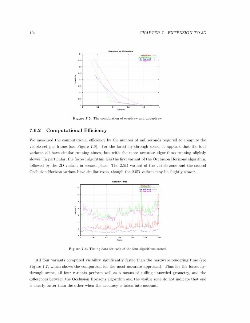
104 CHAPTER 7. EXTENSION TO 3D
0
0.05
0.1
0.15
0.2
0.25
0.3
0.35
0.4
0 0.2 0.4 0.6 0.8 1
Un
der
dra
w
Overdraw
Overdraw vs. Underdraw
2D algorithm2.5D algorithmOH Approx #1OH Approx #2
Figure 7.5. The combination of overdraw and underdraw.
7.6.2 Computational Efficiency
We measured the computational efficiency by the number of milliseconds required to compute the
visible set per frame (see Figure 7.6). For the forest fly-through scene, it appears that the four
variants all have similar running times, but with the more accurate algorithms running slightly
slower. In particular, the fastest algorithm was the first variant of the Occlusion Horizons algorithm,
followed by the 2D variant in second place. The 2.5D variant of the visible zone and the second
Occlusion Horizon variant have similar costs, though the 2.5D variant may be slightly slower.
0
2
4
6
8
10
12
14
0 50 100 150 200 250 300
Tim
e (m
s)
Frame
Visibility Times
2D algorithm2.5D algorithmOH Approx #1OH Approx #2
Figure 7.6. Timing data for each of the four algorithms tested.
All four variants computed visibility significantly faster than the hardware rendering time (see
Figure 7.7, which shows the comparison for the most accurate approach). Thus for the forest fly-
through scene, all four variants perform well as a means of culling unneeded geometry, and the
differences between the Occlusion Horizons algorithm and the visible zone do not indicate that one
is clearly faster than the other when the accuracy is taken into account.

7.7. EXTENSIONS 105
0
20
40
60
80
100
120
140
160
0 50 100 150 200 250 300
Tim
e (m
s)
Frame
Running Times for 2.5D Algorithm
RenderingVisibility
Figure 7.7. The time required by the most accurate variant compared to the rendering time.
7.7 Extensions
The approach described in this chapter for applying the visible zone to a 3D scene can be extended
in several ways, including the following.
1. There is no need to restrict the scene objects to lie on the ground plane: the 3D radial sweep is
a truly 3D algorithm, and the projections of the objects onto the ground plane can be treated
in the same way for the visible zone regardless of their height, as long as the projections do
not overlap. Overlapping projections would require special handling, as briefly discussed in
chapter 4.
2. Many visibility algorithms make use of a hierarchical structure. For example, the Occlusion
Horizons algorithm does not use a global bound on the height of buildings, but instead builds
a quad-tree or similar hierarchy on the set of scene objects that includes height information
for sets of objects. To incorporate a hierarchy in the visible zone algorithm, a group of convex
objects in a convex volume could be treated as a single object, and the transformation between
different levels of a hierarchy could be treated in the same way as the insertion and deletion
of SP-objects in the sweep plane. This appears to be easier in the corner arc algorithm, where
the spatial subdivision is always planar.
3. It may be possible to include some form of temporal coherence in the 3D radial sweep. If the
point observer moves only a small distance, the difference between the 3D radial sweeps at the
two locations may be small, and hence it may be possible to cache information that speeds up
the sweep. Such an improvement could be leveraged by moving the observer near the expected
position at the next frame, doing a 3D radial sweep from the expected position as the objects
of the previous frame are rendered, and then move the observer a yet smaller distance to the
correct position as soon as the correct position is known.
106 CHAPTER 7. EXTENSION TO 3D
It remains to be seen whether such extensions would significantly enhance the efficiency of this
approach for more general types of scenes.
7.8 Conclusion
Computing visibility in a 3D scene is significantly more challenging than in 2D, yet 2D approaches can
still be useful for accelerating low-level operations in 3D algorithms. In a side-by-side comparison of
an algorithm based on the visible zone that computes a 3D radial sweep with the Occlusion Horizon
algorithm of Downs et al. [DMS01], both algorithms performed similarly. The advantage of using
temporal coherence may be tempered by the complexity of the data structures required and by the
constant time costs of low level primitive calculations. Additional research will be required to see if
both of these costs can be reduced or circumvented entirely.
Chapter 8
Conclusion
The investigation of temporally coherent visibility given in this dissertation interweaves local prox-
imity, such as is found between successive observer positions from one frame to the next, and the
geometry of lines, which are responsible for the non-local characteristics of visibility. In general,
one might describe the approach taken as one of embedding the portion of ray-space relevant to a
moving observer in a spatial subdivision. The visible zone does this directly, while the corner arc
invariant embeds a topological equivalent. This approach works well in the plane, where the space
of points and the space of lines have the same number of dimensions. In 3D, where the space of
lines is four-dimensional, we have not been able to find an analogous embedding with acceptable
constant factor costs. Instead, it may be enough in many cases to make approximations that depend
on projections of scene objects into a common ground plane.
8.1 Summary of Results
The visibility complex provides a natural context for understanding and developing exact visibility
algorithms for both static and moving objects. We have described a linear-size substructure of the
visibility complex, called the visible zone, which can be used to maintain the visibility of a moving
observer in a scene of static objects. By generalizing well-known algorithms in computation geometry,
this approach enables worst-case analysis in terms of elements of the visibility complex. In addition,
the most simple associated spatial data structure generalizes the well-known radial subdivision of
the plane, and introduces a variation on spatial subdivisions in which a non-hierarchical set of cells
is permitted to overlap to a limited extent. This spatial subdivision is a first example of an oriented
spatial subdivision in the plane, where the cells of the subdivision can approximate the shape of the
visibility polygon using a number of elements proportional to the combinatorial size of the visibility
polygon.
Although the visible zone can be extended to handle moving occluders, doing so is neither
107

108 CHAPTER 8. CONCLUSION
direct nor necessarily efficient. Instead, a different orientable spatial subdivision – namely a pseudo-
triangulation that embeds the shape of the visibility polygon via corner arcs – can be used to
maintain visibility among moving obstacles in the plane. The corner arc algorithm is simple to
describe, updating the spatial subdivision only in a close neighborhood of the visibility polygon. For
a particular average case setting of randomly placed objects, the corner arc algorithm has nearly-
optimal expected costs, requiring a nearly-constant amount of computation to update the spatial
data structure per change in visibility, for dense or sparse scenes (up to a poly-logarithmic factor).
This is true even when all the objects in the vicinity of the observer (those close enough to have a
reasonable probability of being visible) are moving. Thus, through the use of temporal coherence,
the asymptotic complexity of visibility maintenance in a certain class of average scenes is the same
(up to a poly-logarithmic factor) for static and moving sets of objects.
The analysis of the visible zone and corner arc algorithms indicate the possibility of scaling to
large numbers of objects. In practice, this claim has been verified through implementations using
up to millions of objects. The total cost of handling a change in visibility in our implementation is
approximately 100,000 CPU clock cycles in a static scene, and one million clock cycles for a fully
dynamic scene. Specific estimates for the complexity of handling different event types for average
case scenes are given, which provide a description of the combinatorial structure of visibility in the
neighborhood of the observer for a randomly distributed scene.
In order to extend these results to 3D, we focus on those scenes where the geometry lies close
to a given ground plane. In such a setting, we propose a framework of blended algorithms: using a
fully 3D visibility algorithm at a high level, while processing low-level queries using the temporally
coherent planar visibility query structure of chapter 3. This approach has also been implemented,
and appears to work well for an interactive fly-through of a forest of hundreds of millions of polygons.
In this setting, the time required for visibility calculation is similar to that required by the algorithm
of Downs et al. [DMS01].
8.2 Limitations
The analysis presented here has focused on scenes where objects are randomly placed in a roughly
uniform manner. Naturally, some scenes are not well approximated in this way. For example, in
an urban setting with a grid of streets, the changes in visibility which occur while crossing a street
can be more numerous than traveling a comparable distance in a randomly generated scene. In
worst-case scenarios, the number of changes in visibility, as well as the cost per change in visibility,
can be very high. It may be possible to improve the efficiency of these algorithms for worst-case
scenarios, for example by stepping out of the kinetic framework and re-initializing the structure
when too many events are about to be processed. Such modifications are not explored here.
A second limitation of these methods pertains to the modeling of motion. A very simple motion

8.3. RELATION TO PRIOR RESEARCH 109
model has been proposed that does not leverage motion hierarchies, repeated motion, or motion
constrained to known paths or maximum speeds. These types of motion, which can be found in
scenes of practical interest, can potentially result in substantial savings in computation.
A third limitation has been discussed in the context of extensions to 3D: we have not found
an exact, fully three-dimensional approach to leveraging temporal coherence that avoids expensive
low-level computations. The exact algorithms we propose have significant constant factor costs even
in 2D, and the most promising extension we have found depends on projecting object positions from
space into the plane. As a result, the algorithms proposed here will not work well for 3D scenes that
are not close to some ground plane or that have too many small occluders.
8.3 Relation to Prior Research
The framework for visibility methods proposed in this dissertation is built on the ground-breaking
work on the visibility complex [PV96a] and Kinetic Data Structures [BGH99]. The combinatorial
structures used to construct the visibility complex [PV96a] include a linear-sized sweep structure (the
anti-chain) and an associated spatial subdivision (a pseudo-triangulation). The visible zone derives
from a slight generalization of that sweep structure, and the corner arc algorithm depends on some
of the properties of pseudo-triangulations. These combinatorial structures are combined with the
design approach of Kinetic Data Structures to produce methods for handling moving objects. The
analysis of average case complexity begins with the setting proposed in [COFHZ98], where objects
are distributed nearly uniformly at random, subject to a non-overlapping constraint. The general
method proposed for using an exact planar algorithm in a complex 3D scene resembles many other
approaches for urban settings, including [DMS01]. The observations on the difficulty of obtaining
oriented spatial subdivisions in 3D with low update times draw from work on three-dimensional
KDSs, particularly BSP trees [Mur98] [Com00]. In addition, the work by Joao Comba [Com00]
pointed out the possibility of taking a spatial subdivision that is normally defined with reference to
infinity, and redesigning it around a moving observer.
8.4 Future Work
An immediate continuation of this work would be to generalize the corner arc algorithm to 3D settings
using the general approach given in chapter 7 for transforming a 2D algorithm to an environment
lying near a ground plane. This would arguably be the first 3D, outdoor visibility algorithm that
handles large numbers of moving occluders and focuses on temporal coherence. Additional imple-
mentations could make use of these ideas in a ray-tracing setting or for fast visibility pre-processing
in static scenes. For example, by moving a virtual observer quickly through a static scene during
preprocessing, it may be possible to identify those areas where visibility is particularly complex, and

110 CHAPTER 8. CONCLUSION
then focus the development of acceleration structures there.
The work on extending exact algorithms to complex 3D scenes has underlined the importance of
computing appropriate approximations to the occlusion properties of complex 3D objects. Various
proposals have already been made for such constructions, especially in the plane [KCCO00]. New
approximations may also be helpful for moving occluders.
For the sake of truly general-purpose 3D algorithms, it remains to be seen if the z-buffer can
be used to accelerate computations that take continuous occluder motion into account. Hopefully
some of the insights of theoretical approaches can help to formulate appropriate sampling strategies
which can leverage hardware acceleration.
Amazingly, the venerable problem of efficient visibility computation continues to elicit new and
more efficient algorithms and data structures.

Appendix A
Zone Propogation Lemma
The correctness of the event-finding procedure in chapter 3 depends on the combinatorial relation-
ships between faces of a visibility complex. In order to describe these relationships, we focus attention
on the connectivity of the edges of the visibility complex through the four types of vertices. After
defining various elements of the visibility complex, we describe a geometric tool that can be used
to prove properties of the visibility complex, namely various types of paths through the visibility
complex. Using this tool, we finally prove the zone propogation lemma.
A.1 Towers and Spiralettes
While the visibility complex as a whole can be difficult to visualize, the set of all maximal segments
that intersect the boundary of a given object F is topologically equivalent to a torus, and thus if we
focus on this subset of the visibility complex, our investigations will proceed more easily.
Definition A.1.1. The tower of a object F is the set of maximal segments with an endpoint on
F .
Definition A.1.2. The spiralette of a object T is the set of maximal segments tangent to T .
The boundary of the tower of an object is the spiralette of the object.
A.2 Elements of a Single Tower
We will often find it useful to restrict our attention to the elements of a single tower, and ignore their
relationships to any parts of the visibility complex not represented on that tower. For example, we
know that a edge is on the boundary of three faces, but on a single tower, such a edge appears to only
be on the boundary of two faces, at most. In order to handle this formally, we define counterparts to
111

112 APPENDIX A. ZONE PROPOGATION LEMMA
the elements of the visibility complex defined above, but with the proviso that they are considered
with reference to a particular tower.
Definition A.2.1. A forward tower face is a face, as associated with the forward tower of the
face.
Definition A.2.2. A tower spiralette is a spiralette, as associated with one of its two adjacent
towers.
Definition A.2.3. A forward tower edge is a edge contained in a forward tower, as associated
with that forward tower.
Tower edges are thus restricted not to lie on the boundaries of their associated towers.
Lemma A.2.4. A tower edge lies on the boundary of two tower faces.
Proof: This is an example of the use of these specialized definitions, where the associated towers
of the various tower elements are assumed to be the same. The lemma follows from an examination
of the neighborhood of one of these tower edges, as was done to count the number of faces next to
a edge. ¤
Definition A.2.5. A tower vertex is similarly a vertex, as associated with a tower containing it.
A.3 Spiral Edges and Edge Types
Definition A.3.1. A spiral edge is a maximal connected set of maximal segments, in the inter-
section of a tower and a spiralette.
A edge is exactly the intersection of the two spiral edges (one on each of two towers) which
contain it. Thus, the upper and lower vertices of an edge can be found at one or the other end of
one of the associated spiral edge(s).
Definition A.3.2. A left spiralette is a spiralette whose maximal segments lie locally to the left of
the object of the spiralette, relative to the orientation of the maximal segments. A right spiralette
is a spiralette whose maximal segments lie locally to the right.
This division into ‘left’ and ‘right’ spiralettes also applies to edges and tower edges:
Definition A.3.3. A left edge is an edge whose spiralette is a left spiralette. A right edge is an
edge whose spiralette is a right spiralette.
Definition A.3.4. A left tower edge is a tower edge whose associated edge is a left edge. A right
tower edge is a tower edge whose associated edge is a right edge.
A.4. PATHS 113
A.4 Paths
Perhaps the most useful tool restricted to a single tower is a simple curves in the space of maximal
segments of the tower.
Definition A.4.1. A path on a tower T is defined as follows: Let f be an injective continuous
non-stationary function from a closed interval I of the real numbers to the closure of the set of
maximal segments T , such that any vertex is intersected by the path at most a finite number of
times, and such that the set of real numbers mapped to any edge constitutes a finite number of
subintervals of I. The tower distance is used for the definition of continuity. We call the function
f a path, and we also call the set of segments f(I) a path. In the latter case, we always assume a
particular underlying function f , and by implication the total order on the set of segments implied
by the domain of f .
We also will sometimes use more general paths of segments that are not necessarily maximal
segments, but whose forward or back endpoints remain on the closure of a particular tower T .
A.5 Shapes of Spiralettes and Edges
Lemma A.5.1 (Tower Spiralette Shape). Given a tower spiralette ts associated with tower T ,
let PT be the object of T . Let c be the curve of intersections of the maximal segments of ts with
the object PT . Then c proceeds monotonically counter-clockwise around PT as the height of the
maximal segments increases.
Proof: Omitted. ¤
Definition A.5.2. The supporting ray of a maximal segment m on a forward tower T is the ray
in the plane with origin at the forward endpoint of m, directed so as to contain the back endpoint of
m. Similarly, the supporting ray of a maximal segment m on a tower spiralette s of a forward tower
T whose object is PT , is the ray in the plane with origin at the intersection of m and PT , directed
so as to contain the back endpoint of m. Note that the supporting ray has no associated angle– it
is merely a set of points in the plane.
Lemma A.5.3 (Supporting Ray). The supporting rays of the maximal segments of a tower spi-
ralette are pairwise disjoint, and together cover a sector of the plane bounded by the object.
Proof: Any point of the given plane sector may have either one or two undirected tangent lines to
the associated object, but if there are two, then they will correspond to different spiralettes. ¤
Lemma A.5.4 (Tower Edge Shape). Given a tower edge e associated with a tower T , let PT be
the object of T . Let c be the curve of intersections of the maximal segments of e with the object

114 APPENDIX A. ZONE PROPOGATION LEMMA
PT . Then c proceeds monotonically clockwise around PT as the height of the maximal segments
increases.
Proof: Application of the supporting ray lemma. ¤
A.6 Vertex Types
Vertices can be locally distinguished by the types of the spiralettes to which they belong. The name
of a vertex type is then the (shortened) type of its forward spiralette (left or right), followed by
the (shortened) type of its back spiralette (left or right). Thus there are four types of vertices,
corresponding to the four types of elementary steps.
Definition A.6.1. The forward object of a vertex that belongs to a forward tower is the object
of the forward tower, and the back object of a vertex that belongs to a back tower is the object of
the back tower.
Lemma A.6.2. A vertex v with two tangent points is on the boundary of six faces: one face for
which v is the highest maximal segment of the boundary of the face, one face for which v is the
lowest maximal segment of the boundary of the face, and four faces for which v is locally neither
highest nor lowest along the boundary. Each of these faces has a pair of edges on its boundary which
contain the vertex in their closures.
Proof: Follows from examining the neighborhood of each type of vertex, namely the (left, right),
(left, left), (right, left), and (right, right) vertices. Any pair of the forward, back, forward spiral,
and back spiral objects have a face between them, adjacent to the vertex. ¤
A.7 Types of Faces
Definition A.7.1. A tower edge on the left chain of a forward tower face is a tower edge on the
boundary of the tower face, which is locally to the left of the face, as it appears on the forward
tower. Tower edges on the right chain are defined similarly, but are locally to the right.
Proof: By examining the neighborhood of a maximal segment on a edge, we can verify that the
same tower face always appears to one side of the tower edge, and cannot also appear on the other
side. ¤
Definition A.7.2. The maximal vertex of a face is the maximal segment of the boundary of the
face whose height is maximal. The minimal vertex of a face is defined similarly, but with minimal
height.

A.7. TYPES OF FACES 115
Proof: The above lemma ensures that these are unique. ¤
Definition A.7.3. The left chain of a face is the connected set of vertices and edges on the
boundary of the face between the minimal and maximal vertices, and lying locally to the left of the
face (relative to the direction of the constituent maximal segments). The right chain is defined
similarly, but lying to the right.
Definition A.7.4. A side chain of a face is either the left chain or the right chain.
Definition A.7.5. The forward subchain of a side chain is the set of edges (if any) on the side
chain whose maximal segments are tangent to the forward object of the face, together with any
vertices on the boundary of two such edges. The back subchain is defined similarly, but with
respect to the back object of the face.
Definition A.7.6. The blocking subchain of a side chain is the set of edges which are not on the
forward or back subchains of the side chain, together with any vertices on the boundary of two such
edges.
Definition A.7.7. A blocking edge of a face is a edge on one of the two blocking subchains.
Forward edges and back edges are similar, but are on forward and back subchains, respectively.
Definition A.7.8. A blocking face of a face f is a face on the opposite side of a blocking edge of
f from f .
Lemma A.7.9. The union of the elements of a subchain forms a connected set of maximal segments.
Proof: Follows from closer examination of the traversal argument given above. ¤
Lemma A.7.10. The types of edges found on the various subchains are as follows:
subchain edge types
subchain edge type
left forward left
left blocking right
left back left
right forward right
right blocking left
right back right
Proof: By local structure. ¤
Lemma A.7.11. A side chain consists of one of the following combinations of subchains:
116 APPENDIX A. ZONE PROPOGATION LEMMA
side chain types
forward blocking back
a. present present
b. present
c. present present
d. present present
e. present present present
Proof: Also from the traversal argument. ¤
A.8 Tower Trees and the Face Order
Definition A.8.1. The right tower tree of a forward tower is the tree of vertices and edges formed
by the closures of the right tower edges, together with the left spiralette. The left tower tree is
similar, but with right tower edges and the other tower boundary.
Proof: To prove that these edges form a tree, we first show acyclicity: if there were a cycle, it would
have a minimal height vertex. But such a minimal vertex cannot exist, due to the forward tower
vertex types. Next we show that this is not a forest: Given maximal segments on the indicated
boundary of the tower, there is a unique path joining them along the spiralette(s). An tower vertex
in the right tower tree is connected to the spiral by an increasing height path, which always moves
clockwise, according to the tower edge shape lemma, and cannot stop before the tower boundary,
due to the tower vertex types. However, the spiralettes either stay put or move counter-clockwise,
according to the spiralette shape lemma. Therefore this path must reach a tower spiralette, and we
can connect any two vertices with a unique path. ¤
Definition A.8.2. The face order is the total order on the tower faces of a tower, obtained by
the transitive closure of the above/below relationship of two adjacent tower faces.
Proof: The maximal vertex of a face is a maximal segment in the right tower tree. The face order is
equivalent to the order of the vertices in the right tower tree obtained via an in-order traversal. ¤
A.9 Spiral Edges
We have already seen the definition of a spiral edge, namely a maximal connected set of maximal
segments, in the intersection of a tower and a spiralette. Also, we have seen that forward spiral edges
lie on forward towers, and back spiral edges lie on back towers. We also previously distinguished
between left and right spiralettes. The same distinctions apply to spiral edges, so there are left and
right spiral edges.

A.10. CHORDS 117
Definition A.9.1. A generalized spiral edge is a spiral edge or a tower spiralette.
Definition A.9.2. The terminating vertex of a spiral edge is the highest maximal segment of
its closure. Similarly, the initiating vertex of a spiral edge is the lowest maximal segment of its
closure.
Definition A.9.3. The terminating edge of a spiral edge is the generalized spiral edge of the
same tower that contains its terminating vertex. The initiating edge is the generalized spiral edge
of the same tower containing for its initiating vertex.
Lemma A.9.4. The terminating edge of a forward spiral edge is either a right spiral edge or a
tower spiralette of the terminating tower spiral. Similarly, the initiating edge of a forward spiral
edge is either a left spiral edge or a tower spiralette of the initiating tower spiral.
Proof: By examination of the vertex types. ¤
The terminating edge of a back spiral edge is either a left spiral edge or a tower spiralette of the
terminating tower spiral. Similarly, the initiating edge of a back spiral edge is either a right spiral
edge or a tower spiralette of the initiating tower spiral.
Lemma A.9.5. A forward right spiral edge has only one tower face locally to its left, and a forward
left spiral edge has only one tower face locally to its right.
Proof: Follows from the previous lemma. ¤
Lemma A.9.6. Let s be a forward spiral edge terminating at a vertex v, where v is not on the
tower boundary. The terminating edge is part of the forward spiralette of v. Similarly, the initiating
edge is part of the forward spiralette or spiralette of the initiating vertex.
Proof: By examination of the vertex types. ¤
Lemma A.9.7 (Spiral Edge). The upper vertex of an edge is the terminating vertex of either its
forward or back spiral edge.
Proof: Follows from the definition of these edges. ¤
A.10 Chords
Definition A.10.1. A chord is a segment in free space, whose endpoints are on objects, and whose
interior is disjoint from all object boundaries.

118 APPENDIX A. ZONE PROPOGATION LEMMA
Lemma A.10.2. The relationship between two chords must be one of the following: 1) they are
disjoint 2) they are identical 3) their intersection consists of an endpoint of both 4) they cross in
the interior of both.
Proof: The only possibilities for intersection that are disallowed involve the endpoint of one chord
lying in the interior of the other, which cannot happen because that point must either lie on an
object boundary or not. ¤
Definition A.10.3. The forward tower segment of a maximal segment of a forward tower or a
maximal segment of a tower spiralette of a forward tower is the chord contained in the supporting
ray for that maximal segment and that tower, that includes the origin of the supporting ray.
Convention: The mapping from a chord to a maximal segment is represented by subscripting
the letter m of the maximal segment with the chord. For example, if c is a chord, then mc is a
maximal segment containing c.
Definition A.10.4. The intersection of a maximal segment with a object, or with another max-
imal segment, is the intersection of these objects when considered as sets of points in the plane.
For example, one maximal segment intersects another maximal segment if, when considered as
segments in the plane, they have at least one point in common.
Convention: When the name of a maximal segment is subscripted with the name of a object,
the resulting symbol is used to denote the point in the plane where the maximal segment intersects
the the object. For example, if v is a maximal segment, and F is a object, then vF is the intersection
point of v and F .
Lemma A.10.5 (Face Chord). Let c be a chord intersecting a maximal segment m of a face
f between objects B and F . Then the set of maximal segments of f intersecting c includes the
following:
1) If the endpoints of c do not lie on B or F , then all maximal segments of f intersect c.
2) Otherwise, let qF be the maximal connected set of boundary points of F consisting entirely of
forward endpoints of maximal segments of f , excluding any endpoint of c, but including the forward
endpoint of m. Let qB be the analogous set on B. Then all the maximal segments of f whose
endpoints lie in both qF and qB must cross c.
Proof: For case 1, let p be a path lying in the interior of f , starting at m, and ending at any other
segment n of f . Since this path does not involve any maximal segments tangent to a object, the
constituent maximal segments of this path are all chords. By delta arguments, the only way for a
continuously moving chord to cease intersecting a static chord is for the moving chord to share an
endpoint with the static chord. However, the endpoints of the chords of p are on different objects
A.11. FORWARD PATHS 119
than the endpoints of c, so this can never happen. Thus all such paths consist of chords intersecting
c.
For case 2, suppose c touches both F and B. Let pF be the path of segments in f whose forward
endpoints coincide with cF (note the use of the above convention here), and pB be the path of
segments in f whose back endpoints coincide with cB . According to our results on the shape of a
tower face, these paths each divide f into two parts, each of which is a topological disk of segments.
In addition, these two paths intersect at most once, since there can be at most one maximal segment
containing both cF and cB . Thus together they divide f into four topological disks, corresponding
exactly to those segments which intersect both qF and qB , just one of them, or neither. Since m lies
in the region of maximal segments intersecting both qF and qB , and since any path in this region
cannot have a maximal segment sharing an endpoint with c, then all these maximal segments must
intersect c.
The argument for when c intersects F or B, but not both, is similar, only now it is not necessary
to argue about the intersection of two parts of f . ¤
A.11 Forward Paths
Lemma A.11.1 (Path Interval). If all the segments of an open interval of segments on a path
have the same segment type, then they are all on a single edge, or in a single face. Furthermore,
there exists an open interval of segments of the path on each side of the segment, each of which
consists of maximal segments of a single segment type.
Proof: The first assertion follows from the non-stationary requirement on paths, together with the
definitions of edges and faces. The second assertion follows from the fact that a path passes through
a finite number of vertices, edges, and faces, a finite number of times each, and from the topology
of the real interval which is the domain space of the path. ¤
Lemma A.11.2 (Type Transformation). Let p be a path that lies entirely on a edge or in a
face, except for the last segment v of p. Let x be the limit point of the forward endpoints of the
segments of p leading up to v, and let y be the limit point of the back endpoints of the segments of
p leading up to v. Let s be the segment from x to y. Then s is one of the chords contained in v, or
the union of adjacent chords in v.
Proof: By examination of the local geometry of the various edge and vertex types. ¤
Definition A.11.3. A forward path is a path on a forward tower whose maximal segments have
been replaced by the forward tower segments of those maximal segments. That is, a forward path
satisfies the properties of a path in general, but consists of chords with one endpoint on a particular
forward tower.

120 APPENDIX A. ZONE PROPOGATION LEMMA
Lemma A.11.4. The forward endpoints of the segments of a forward path move continuously.
Proof: In this report, the movement of segments or endpoints refers to the ordered set of segments or
endpoints obtained from a path or a composition of another function with a path. In the definition
of a path, the tower distance was used for the definition of continuity, which measures distances
between the forward endpoints of the segments of the corresponding forward path, and thus implies
continuous movement of the endpoint when viewed simply as a point in the plane. ¤
Lemma A.11.5 (Forward Path Lemma). Let p be a forward path starting with forward tower
segment a. Let b be a chord, such that a and b do not intersect. If any of the forward tower segments
of p intersects b, then let c be the infimum of the set of all such segments of p that intersect b. Then
the relationship between b and c can be described in one of the following ways:
1) b = c
2) b and c share an endpoint.
3) mc intersects the interior of b, but c doesn’t intersect b. Also, the length of the segments of p
in a neighborhood of c increases discontinuously at c.
Proof: We first note that since we are only considering forward segments of the path p, we are always
dealing with chords. Consider the motion of the back endpoint of the forward tower segments of
p. If this motion is continuous at c, then c must be a chord sharing an endpoint with b, following
an argument similar to that used for the face chord lemma. If it is not continuous at c, then by
delta arguments, the chords cannot be discontinuously decreasing in length at c, and still manage
to intersect b immediately thereafter. The only way for the back endpoint of the segments of p to
move discontinuously is at a segment type change. We have examined these type changes in the type
transformation lemma, where we saw that they appear locally like the addition or deletion of chords
from a maximal segment on the boundary of a face. Thus to increase in length discontinuously
involves the apparent addition of a chord at a maximal segment on the boundary of a face, such
that the chord previously present was not intersected. ¤
A.12 Diagonal Paths
Definition A.12.1. A diagonal path on a forward tower is a path which is strictly monotonic
in height and in position on the tower. In addition, a diagonal path must proceed either up and
clockwise, in which case it is called an increasing diagonal path, or down and counter-clockwise,
in which case it is called a decreasing diagonal path.
Lemma A.12.2. A spiral edge is a diagonal path.
Proof: Follows from the tower edge shape lemma, together with the local structure of tower ver-
tices. ¤

A.13. CONSERVATIVE PATHS 121
Lemma A.12.3 (Diagonal Path Lemma). Consider two diagonally placed forward tower seg-
ments a and b on a forward tower, such that they do not intersect. Consider also a diagonal forward
path p starting from a, directed toward b. If any of the segments of p intersects b, then let c be the
infimum of the set of all segments of p that intersect b. Then the relationship between b and c can
be described in one of the following ways:
1) c is b
2a) c shares the forward endpoint of b. If p is a decreasing (increasing) path, then c has lesser
(greater) height than b.
2b) c shares the back endpoint of b. If p is a decreasing (increasing) path, then c has greater
(lesser) height than b.
3) mc intersects the interior of b, but c does not intersect b. Also, the length of the segments of
p in a neighborhood of c increases discontinuously at c.
Proof: This is a specialization of the forward path lemma, but taking height into account. For
2a), assume otherwise. Then by delta arguments, forward segments of p must intersect b just before
reaching c. For 2b), we must intersect b at or before the first time that the forward endpoint of the
segments of p reaches the forward endpoint of b, but in the disallowed case, the forward endpoint of
c is on the opposite side of b from the forward endpoint of a. ¤
A.13 Conservative Paths
Definition A.13.1. A conservative path is a forward path satisfying the following property: the
mapping from the path to the lengths of the segments of the path is a continuous mapping, except
where the length is discontinuously reduced.
Lemma A.13.2 (Conservative Path Lemma). Let p be a conservative path starting with tower
forward segment a. Let b be a chord, such that a and b do not intersect. If any of the segments
of p intersects b, then let c be the infimum of the set of all segments of p that intersect b. The
relationship between b and c can be described in one of the following ways:
1) b = c
2) b and c share an endpoint.
Proof: This is a different specialization of the forward path lemma, where we eliminate the option
of increasing the segment length discontinuously. ¤
A.14 Branches
Definition A.14.1. The up branch of a forward spiral edge on a forward tower is the path obtained
by following the spiral edge up to its terminating vertex, and doing the same for the terminating

122 APPENDIX A. ZONE PROPOGATION LEMMA
edge thus found, and repeating, until the tower boundary is reached.
Definition A.14.2. The down branch of a forward spiral edge on a forward tower is defined
similarly, only this time we follow the spiral edge down to the initiating vertex, and repeat.
Definition A.14.3. A branch is an up branch or a down branch.
Lemma A.14.4. A down branch has at most one right spiral edge, and an up branch has at most
one left spiral edge.
Proof: According to the local tower vertex geometry, terminating vertices not on the tower bound-
ary only occur on right spiral edges, and initiating vertices off the boundary occur only on left spiral
edges. ¤
Lemma A.14.5. A branch is a diagonal path.
Proof: Follows from the spiral edge shape lemma. ¤
Lemma A.14.6. A branch is a conservative path.
Proof: Follows from the local geometry of terminating vertices, which was examined earlier. ¤
Definition A.14.7. A branch path is the forward path associated with a branch on a forward
tower.
Lemma A.14.8 (Branch Path Lemma). Consider two diagonally placed, non-intersecting for-
ward tower segments a and b on a forward tower, such that a lies on a edge, and b lies either on
a edge or on a vertex. Consider also a branch p starting from a, directed toward b. If any of the
segments of p intersects b, then let c be the infimum of the set of all segments of p that intersect b.
Then the relationship between b and c can be described in one of the following ways:
1) b = c
2a) c shares the forward endpoint of b. If p is a decreasing (increasing) path, then c has lesser
(greater) height than b.
2b) c shares the back endpoint of b. If p is a decreasing (increasing) path, then c has greater
(lesser) height than b.
Proof: This is just the result of merging the conservative path lemma with the diagonal path
lemma. ¤
Lemma A.14.9. Let e be a forward spiral edge, whose terminating vertex v does not lie on the
tower boundary. Let et be the terminating edge. Let b be the forward tower segment of a maximal
segment of e, and let c be the forward tower segment of a maximal segment of et. Let a be forward
tower segment diagonally placed with respect to b, with angle less than b. If a intersects c, then a
intersects b.

A.14. BRANCHES 123
Proof: Let F be the forward object of v, which is thus the object of the forward tower on which
all these segments lie. Let C be the object containing the forward spiral point of v, which is then a
tangent point according to the possible types of interior terminating vertices. If v does not intersect
b then let B be the object of the spiralette of b, which then also contains the back spiral point of v,
according to the possible types of termination vertices.
Let R1 be the region of the plane bounded by c, the part of F between cF and vF , v∗, and the
part of C between vC and cC , if this is not just a point. Similarly, if v does not intersect b, then let
R2 be the region of the plane bounded by b, the part of F between bF and vF , the part of v from
vF to vB , and the part of B from vB to bB . If v intersects b, then let R2 be the region of the plane
bounded by b, the part of F from bF to vF , and v.
Let y be the intersection point of a and c. Since b and c are diagonally placed, and a and b are
diagonally placed, a and c are also diagonally placed forward tower segments on the same forward
tower. Thus the forward endpoint of a, aF , occurs forward of y on a. Since a is a chord, this means
that a does not intersect any object other than F forward of x.
Also, since a and b are diagonally placed, aF does not lie between bF and cF on F , but instead
lies counter-clockwise of these points along F .
Now a enters R1 at y, and cannot stop on the boundary of F along R1, so a must then exit R1
at a point z on v. But that means that a enters R2 along v. Again, a cannot stop on the boundary
of F along R2, so a must exit R2 along b. This is what was to be demonstrated. ¤
Lemma A.14.10 (Branch Space). Any two segments on a branch path do not intersect each
other on in their interiors.
Proof: We examine only the case of up branches, since the case of down branches is symmetric.
Suppose the lemma is false, and let p be an up branch path with at least one pair (a, c) of chords
on it that intersect. Assume WLOG that a is the lower segment of the pair. For now, let us also
assume that neither a nor c is a vertex.
By the supporting ray lemma, two forward tower segments on a single spiral edge do not intersect.
So a and c must be on different spiral edges, say e0 and et, respectively. Let e be the spiral edge of
p just below et, and let v be the terminating vertex of e on et. Let b be a forward tower segment of
e between a and c. Now we apply the preceding lemma, which shows that a must also intersect b.
However, if we can do this once, we can do it again, and again, until b lies on e0. Thus we have a
contradiction, because we have found another forward tower segment on e0 that intersects a. Thus
the initial assumption, that a intersects c, is impossible.
Finally, if a and/or c is part of a vertex, then we can apply delta arguments to show that they
have nearby neighbors that intersect, yielding the conclusion that even in these special cases, a
cannot intersect c. ¤

124 APPENDIX A. ZONE PROPOGATION LEMMA
A.15 Branch Face Lemma
Lemma A.15.1. The up branch of a edge e on the left chain of a forward tower face contains the
other edges of the left chain above e, up to the tower boundary. In particular, if the maximal vertex
of the face is not on the tower boundary, then it is on the up branch. Similarly, the down branch of
a edge e on the right chain of a forward tower face contains the other edges of the right chain below
e, up to the tower boundary. In particular, if the minimal vertex of the face is not on the tower
boundary, then it is on the down branch.
Proof: By examination of the types of forward tower vertices. ¤
Lemma A.15.2 (Branch Face). Let t be the terminating vertex of a spiral edge s, and let f be
the tower face locally below t. If the minimal vertex v of f is not on the tower boundary, then v is
on the down branch of s.
Proof: The forward tower segment associated with a maximal segment will be indicated by adding
a superscripted asterisk to the name of the maximal segment. Let e be the edge on the right chain
of f whose upper vertex is t, which may may or may not be on s. If e is on s, then the result follows
immediately from the previous lemma, so in the rest of the proof, assume that this is not the case.
First, t∗ and v∗ do not intersect since they both lie on the downbranch of e, by the branch space
lemma.
Second, the branch path p along the down branch of s contains at least one segment that does
intersect v∗, as follows. Let z be the path of forward tower segments on the forward tower of f , that
share the same forward endpoint as v, but have height greater than or equal to that of v. Since p
always stays on face boundaries, it cannot intersect f on its way down, so it must intersect z. But
this means that it has a segment that shares its forward endpoint with v∗.
Third, by applying the branch path lemma to p and v∗, the only way for p not to contain v∗ is for
p to contain another forward segment c that shares the forward endpoint of v∗, but has lesser height
than v. But the above observation that p must intersect z shows that this would be impossible. ¤
A.16 Zone Propagation
Lemma A.16.1 (Zone Propagation). If f is a zone face of a forward tower whose maximal vertex
t is not on the tower boundary, then the face immediately below t is also a zone face.
Proof: Let g be the face below t, and s the spiral edge terminating at t. If g reaches the initiating
tower spiral, then g must be a zone face, since a left-chain crossing walk from f to the terminating
tower spiral cannot cross the down branch of s, nor can it reach the initiating tower spiral, so it
must cross through g.

A.16. ZONE PROPAGATION 125
On the other hand, if g does not reach the initiating tower spiral, g still must be a zone face,
since we can now apply the branch face lemma to see that the down branch of s must pass through
the minimal vertex of g, and so a left-chain crossing walk from f must similarly pass though g before
reaching the terminating tower spiral. ¤

126 APPENDIX A. ZONE PROPOGATION LEMMA

Appendix B
Elementary Step Sequences
The correctness of the recursive update procedure described in chapter 3 depends on the properties
of sequences of elementary steps that connected different cuts of the visibility complex. Although the
overall shape of the argument for this correctness was given in chapter 3, this appendix presents the
details and also provides a slightly broader analysis of the elementary step sequences and the effect
of motion on the connectivity provided by these sequences. A final section addresses the amortized
worst case bounds claimed for a static scene.
Among possible cuts of the visibility complex, another cut besides the perspective cut defined
in chapter 3 is the vertical cut, whose tangent segments are the segments of vertical trapezoidal
subdivision of the scene. That is, if we consider all maximal segments tangent to an object and
parallel to the y-axis, this set constitutes the vertical cut, and the zone resulting from this cut is
the vertical zone. In the vertical zone, all the faces of the visibility complex containing maximal
segments with infinite extent in the negative y direction are part of the zone, and thus the zone
can be used to identify the lower envelope of the scene. The same can be done with the vertical
decomposition, but a zone has more flexibility: we call a lower envelope zone any zone that can
be obtained by applying elementary steps to the vertical zone, with the constraint that the above
mentioned faces remain in the zone. Thus any lower envelope zone captures the lower envelope of
the scene. A lower envelope zone is somewhat simpler than a visible zone, and so will motivate some
of the analysis.
B.1 Zone Transformations
In order to be able to maintain a zone when the objects of the scene move, the zone needs to be
changed periodically into a related zone. The first subsection below defines a general class of zone
transformations, and shows how to represent a zone transformation as a sequence of sets of vertices.
The second subsection examines ‘composite steps’. The third and fourth subsections demonstrate
127
128 APPENDIX B. ELEMENTARY STEP SEQUENCES
that for two zones z1 and z2 in a static scene, there is at most one such zone transformation from one
zone to the other, modulo some ‘redundant’ operations. The final subsection examines properties of
minimum length transformations from a given zone z to a nearby space of zones.
B.1.1 Definition
The underlying transformation step used in the topological sweep algorithm [PV96a], using the
terminology from [EG86], can be defined as follows. An elementary step is an operation by which
a cut is changed incrementally, by removing two cut edges that share a vertex, and replacing them
with the other two edges incident to the vertex. Note that, if a vertex has a cut edge immediately
below it (according to relative angle), then it cannot have a cut edge immediately above it (and
vice versa), since these two edges would then be on a single side chain of some face. An elementary
step is considered to go upward if it involves replacing edges below a vertex with those above, or
downward if it goes the other way.
An elementary step can be specified with just a vertex, since the location of the zone implies the
direction of the elementary step.
A composite step has a similar definition as an elementary step, but involving more than one
vertex, as follows. Let V be a set of vertices, let I (the interior edges) be the set of edges whose
upper and lower vertices both lie in V , let L (the lower edges) be the set of edges whose upper
but not lower vertices are in V , and let U (the upper edges) be the set of edges whose lower but
not upper vertices are in V . For a given zone z, the set V defines an upward composite step if the
following conditions are met:
1) The edges of L are all cut edges.
2) None of the edges of I or U are cut edges.
3) There is no non-empty proper subset of V satisfying conditions 1) and 2).
The upward composite step consists of removing the set L from the cut, and replacing it with the
set U . A downward composite step is defined analogously. It will be shown elsewhere that applying
a composite step to a cut always results in a cut. A composite step can be specified by the set of
vertices V , since the direction of the composite step (upward or downward) is also implied by the
location of the cut.
A zone transformation T is a finite sequence of elementary and composite steps (or steps, for
short). Thus T can be represented as V1, V2, ..., Vn, where each Vi is a non-empty set of vertices.
B.1.2 Properties of Composite Steps
A composite step is necessarily more complex than an elementary step. Before launching into a
description of zone transformations, let us consider how composite steps may be related to elementary
steps, and what composite steps can occur consecutively in a transformation.

B.1. ZONE TRANSFORMATIONS 129
Lemma B.1.1. For any composite step V , the set of lower edges L and the set of upper edges U
are both non-empty.
Proof: If the set V consists of all the vertices of the visibility complex, then the interior edges of
V include all the edges of the visibility complex, including all cut edges of a zone. Then V would
not be a composite step. Thus there must exist at least one vertex v that is not included in the set
V . Let v′ be a vertex that is in V . Due to the connectivity of the graph of vertices of edges of the
visibility complex, there exists an ascending (locally increasing angle) chain of edges from v to v′.
Let w be the first vertex of V encountered in a traversal of this chain from v to v′. Then the edge
of the chain below w is a lower edge of V . A similar argument establishes the existence of an upper
edge of V . ¤
In the following lemma, as elsewhere, the choice of an upward step is arbitrary; a symmetric
result applies to downward steps.
Lemma B.1.2. Let V be a composite step upward, and let v1 and v2 be any two vertices of V .
Then there exists an ascending chain of interior edges of V connecting v1 to v2 (and vice versa).
Proof: Let V ′ be the set of vertices of V reachable by descending interior edge chains from v2. Let
I, L, and U be the interior, lower, and upper edges of V , respectively.
Let I ′, L′, and U ′ be the interior, lower, and upper edges of V ′, respectively. If e′ is an edge of
L′, then the lower vertex v′ of e is not in V ′, which means that v′ is not in V . Thus e′ must be in L,
and L′ must be a subset of L. The edges of I ′ and U ′ must either be in I or U , since they all have
their lower vertices in V ′, and thus in V . Thus none of the edges I ′ or U ′ are cut edges. If V ′ does
not include all the vertices of V , then we have identified a non-empty proper subset of V satisfying
the first two criteria for a composite step, and thus a contradiction.
Therefore V ′ must include all the vertices of V . In particular, v1 must be in V ′. ¤
Composite steps may thus be thought of as connected chains of edges, which cannot be reduced
to elementary steps because there is no clear starting point.
Lemma B.1.3 (Composite Match). Let V1 and V2 be consecutive composite steps of a transfor-
mation T . If V1 and V2 have at least one vertex in common, then V1 and V2 involve the same set of
vertices, and have opposite directions.
Proof: Let v be a vertex in both V1 and V2.
Case 1: V1 and V2 are both upward steps. Let e be an edge immediately below v. Thus e is a
lower edge or an interior edge of V1, and a lower edge or an interior edge of V2.
If e is an interior edge of V1, then e must also be an interior edge of V2, since after V1, e is not
in the cut, and so cannot be a lower edge of V2. Let v′ be another vertex of V1. By tracing interior
edges down from v to v′, v′ must be in V2 as well. So all the vertices of V1 are found in V2.
130 APPENDIX B. ELEMENTARY STEP SEQUENCES
Let e′ be an upper edge of V1, so it is an upper or interior edge of V2. However, e′ is added to the
cut by V1, so cannot be an upper or interior edge of V2. So there is a contradiction, and there cannot
be two consecutive composite steps in the same direction with at least one vertex in common.
Case 2: V1 is an upward step, and V2 is a downward step. Let e be an edge immediately above
v. Thus e is an upper edge or an interior edge of V1, and an upper edge or an interior edge of V2.
If e is an upper edge of V1, then it must also be an upper edge of V2, since after the step V1, it
is in the cut, and thus cannot be an interior edge of V2.
Conversely, if e is an interior edge of V1, then e must also be an interior edge of V2, since after
applying the composite step V1, e is not in the cut, and e would need to be in the cut to be an upper
edge of V2. Thus e is an interior edge of V1, if and only if e is an interior edge of V2.
Let v′ be another vertex of V1. By tracing interior edges up from v to v′, v′ must be in V2 as
well. Similarly, let v′′ be another vertex of V2. We can connect v′′ to v with a descending chain of
interior edges in V2. By traversing this chain in the opposite direction, we cannot encounter any
upper edges of V1, so v′′ must also be in V1. Thus V1 and V2 involve the same set of vertices.
The other cases, where V1 is a downward step, are similar. ¤
Two consecutive steps in a zone transformation with the same set of vertices (whether elementary
steps or composite steps) are called a redundant pair since their effects on the cut cancel each
other out.
B.1.3 Equivalent Transformations
When a transformation contains a redundant pair, removing this redundant pair from the sequence is
in some sense a trivial adjustment of the sequence. Also, if two consecutive steps of a transformation
operate on completely different parts of the visibility complex, transposing their order in the sequence
(an allowable transposition) is also in some sense a trivial change. An allowable ordering of steps
of a transformation is any ordering obtainable using allowable transpositions.
Definition: Two sequences of steps T1 and T2 that both transform a zone z1 into another zone
z2 are equivalent (T1 ∼ T2) if by allowable transpositions in the order of steps, and the removal of
redundant pairs, T1 and T2 can be reduced to the very same sequence.
Let us begin by examining what can happen to a sequence as allowable transpositions and
deletions of redundant pairs are applied.
Lemma B.1.4 (Transposability). Let Vi and Vi+1 be two consecutive steps of a transformation
T , such that Vi and Vi+1 have no vertices in common, and their directions (upward or downward)
are opposite. Then Vi and Vi+1 have no incident edges in common, and can be transposed in T .
Proof: WLOG let Vi be upward and let Vi+1 be downward. Suppose e is an edge incident to a
vertex of Vi, and suppose that e is also incident to a vertex of Vi+1. Because Vi and Vi+1 are disjoint,
B.1. ZONE TRANSFORMATIONS 131
either e is an upper edge of Vi and a lower edge of Vi+1, or a lower edge of Vi and an upper edge of
Vi+1.
If e is an upper edge of Vi, then e is in the cut just after Vi, which means e is in the cut just
before Vi+1, which means it cannot be a lower edge of Vi+1. Similarly, if e is a lower edge of Vi, then
e is not in the cut just after Vi, so e is not in the cut just before Vi+1, so e is not an upper edge of
Vi+1. Thus there are no edges incident to both Vi and Vi+1.
Therefore Vi and Vi+1 can be transposed, since their requirements and effects on a cut are entirely
independent of each other. ¤
A unidirectional transformation is a sequence of steps that all go up, or that all go down. The
concatenation of two sequences of steps is indicated by, e.g., T1T2.
Lemma B.1.5 (Decomposability). For any transformation T , T ∼ TupTdown, the concatenation
of two unidirectional sequences where the first is composed entirely of upward steps, and the second
is composed entirely of downward steps.
Proof: Consider two steps Vi and Vi+1 of T such that Vi is a downward step and Vi+1 is an upward
step. (If there is no such pair, T already satisfies the lemma.)
If Vi+1 has at least one vertex in common with Vi, then this pair of steps can be deleted from the
sequence, since they form a redundant pair. If on the other hand Vi+1 has no vertices in common
with Vi, then these steps can be transposed.
Finally, such deletions and transpositions can be repeatedly applied until the desired sequence
is obtained. ¤
A non-redundant transformation is a sequence of steps such that no vertex has associated steps
that go both up and down over it.
Lemma B.1.6 (Non-redundancy). For any transformation T , T ∼ T ′, where T ′ is non-redundant.
Proof: In the above proof of the decomposability lemma, redundant adjacent pairs were deleted as
part of the process of rearranging the order of steps of T . By rearranging the order of steps of T so
that all the upward steps occur first, and then rearranging again so that all the upward steps occur
last, all possible pairs of upward and downward steps are at some point transposed with each other,
so that all redundancies are thereby removed. ¤
The above proof also establishes the transitivity of the equivalence relation ∼, since it shows how
to remove all redundancies from a sequence before we even know what other sequence it may be
compared to, leaving only transpositions that need to be performed to make two sequences match
(which in turn are clearly transitive).
A slightly tricky aspect of zone transformations is that there may exist long sequences of steps
that transform a zone z1 into itself. In order to avoid these identity transformations, let us focus

132 APPENDIX B. ELEMENTARY STEP SEQUENCES
for the moment on the case of restricted transformations, which are sequences of steps that are
not permitted to include steps across some predefined non-empty set of vertices (the restricted
vertices). This type of restriction limits the parts of the visibility complex to which a zone can be
moved, and so will also be used in maintaining properties of zones in the applications to be described
later.
Lemma B.1.7. All unidirectional, restricted transformations are of bounded length in the size of
the scene.
Proof: Otherwise, there is a vertex that is traversed an unbounded number of times. This means
that the vertices on the opposite ends of the adjoining edges are also traversed an unbounded number
of times. Because the graph of vertices and edges is connected, applying this reasoning repeatedly,
all vertices must be traversed an unbounded number of times. This contradicts any restriction on
vertices. ¤
A maximal transformation M is a unidirectional, restricted transformation such that no other
unidirectional transformation in the same direction, with the same restriction, properly contains M
as a prefix.
Lemma B.1.8. Any two maximal transformations for a given zone z in the same direction, with
the same restrictions, are equivalent.
Proof: By induction on the length of the shorter transformation. Without loss of generality, let T1
and T2 be two maximal transformations of z with the same restrictions, both going up, with lengths
n and m respectively, such that n ≤ m.
Let V be the first step of T1, let e be a lower edge of V , and let v be the upper vertex of e. Then
e is a cut edge of z, and any step that removes e from the cut must involve the vertex v. If none of
the steps of T2 include v, then e is in the cut at the end of T2. Let e′ be an upper or interior edge of
V , and let v2 be the lower vertex of e′. Then e′ is not a cut edge of z, and any step that adds e′ to
the cut must include v2. If none of the steps of T2 include any of the vertices of V , then at the end
of T2, all the incident edges of V have not changed with respect to the cut, so V could be applied.
This contradicts the maximality of T2, so at T2 must have a step that includes a vertex from V .
In the Move-To-Front lemma below, we will prove that the first such step of T2 involves exactly
the same vertices as V , and can be moved to the front of T2 by allowable transpositions.
If n = 1, T1 has only the one step V . If T2 has length greater than one, and V is moved to the
beginning of T2, then T2 proves that T1 was not maximal, a contradiction. Thus T2 must be the
same as T1, and the claim is verified for n = 1.
Suppose the claim is true for all pairs of maximal transforms of z, where n = k for some k. First
re-arrange the order of the steps of T2 so that V is again the first step of T2.
B.1. ZONE TRANSFORMATIONS 133
Let z′ be the zone obtained by applying V to z. Let T ′1 and T ′2 be two transformations of
z′, which are obtained by removing V from the beginning of T1 and T2, respectively. That these
transformations are unidirectional, in the same direction, with the same restriction as T1 and T2, is
obvious. That they are maximal then follows from the fact that, the zone obtained by starting with
with z and applying T1 is the same as that obtained by taking z′ and applying T ′1, so there are no
valid steps left for either of them at the end of the transformation. The same applies to T2. Now
however we have that T ′1 and T ′2 are allowable permutations of the same steps (in the sense that
the permutations are obtained by allowable transpositions), so T1 and T2 must also be allowable
permutations of the same steps. ¤
The preceding proof made use of the following lemma:
Lemma B.1.9 (Move-To-Front). Let V be an upward step containing a vertex v, that can be
applied to a zone z. Let T be a unidirectional transformation on z, such that T includes at least one
upward step over the vertex v. Then the first step of T that includes v is exactly V , and furthermore,
this step can be moved to the front of T by allowable transpositions.
Proof: Let z′ be the zone obtained by applying V to z, and let T ′ be a zone transformation for z′,
starting with a downward step across the vertices of V followed by the steps of T . Now T ′ has one
downward step, followed by all upward steps. By the transposition lemma, this downward step is
completely independent of all upward steps at the beginning of T ′, up to the first step Vi that has
a vertex in common with V . Also, once V has been transposed as far as Vi, we find that Vi and V
must involve exactly the same vertices. [Therefore there exists only one such step V .]
Let Vi also denote the first occurrence of V in T . According to the preceeding reasoning, Vi has
no incident edges in common with any of the steps of T before it. Thus Vi can be moved to the
beginning of T . ¤
Let T−1 be the sequence Vn, ..., V2, V1, with all the steps taken in the opposite direction as in T .
Clearly, if T transforms z1 into z2, then T−1 transforms z2 into z1. Also, the functional notation
T (z) refers to the zone obtained by applying T to z.
Theorem B.1.10. Given a restricted transformation T from z1 to z2, and two maximal transfor-
mations T1 and T2 in the same direction for z1 and z2 respectively, with the same restriction on
vertices, then the zones obtained by applying T1 and T2 to z1 and z2, respectively, are identical.
Proof: Assume WLOG that T1 and T2 are upward. Let T ′ be a sequence such that T ′ ∼ T and
T ′ = TupTdown, the concatenation of two unidirectional transformations. Let z1,max = T1(z1),
z2,max = T2(z2), and zshared = Tup(z1) = T−1down(z2). Then z1,max = T1(T−1
up (zshared)), and T−1up T1
is a maximal transformation of zshared. Similarly, z2,max = T2(Tdown(zshared)), and TdownT2 is a
maximal transformation of zshared. Now TdownT2 ∼ T−1up T1 as applied to zshared, and so z1,max is
the same as z2,max. ¤

134 APPENDIX B. ELEMENTARY STEP SEQUENCES
In other words, in a space of zones connected by restricted transformations, there is exactly one
maximum.
Theorem B.1.11. For any two restricted transformations T and T ′ from z1 to z2, T ∼ T ′.
Proof: Let T ∼ T ′′ = TupTdown, where the decomposition is also non-redundant. Let Tmax be
an extension of Tup into a maximal transformation, which is the concatenation of Tup with another
transformation Text. T−1extTdown is then the inverse of some maximal transformation, Tmin. Now T ∼
TupTextT−1extTdown = TmaxT−1
min. However, the same construction applies to T ′: T ′ ∼ Tmax′T−1min′ , for
some maximal transformations Tmax′ and Tmin′ . Furthermore, we have from a previous lemma that
Tmax ∼ Tmax′ , and Tmin ∼ Tmin′ . So T ∼ TmaxT−1min ∼ Tmax′T
−1min′ ∼ T ′. ¤
B.1.4 General Sequences
In order to handle the possibility of identity transformations, we focus on characterizing these
identity transformations, and then expand the definition of equivalence to allow for them. If the
visibility complex is defined using maximal segments with angle, then this subsection is unnecessary,
as follows.
Lemma B.1.12. No non-redundant identity transformations exist (except the trivial transforma-
tion of zero steps) when the visibility complex is defined using maximal segments with angle.
Proof: Suppose otherwise, so let T be a non-redundant transformation from zone z to itself with
at least one step. Let T = TupTdown, the concatenation of two unidirectional sequences. Now Tup
must itself be an identity transformation, since by the transposition lemma, all the steps of Tup and
Tdown are independent. So we can assume T is composed entirely of upward steps.
Let V1 be the first step of T . Let e0 be a lower edge of V1, so e0 is a cut edge of z. Let e1 be an
upper edge of V1, connected to e0 by an ascending chain of interior edges of V1.
Now if e1 is not a cut edge of z, let Vj be the next step after V1 that involves the upper vertex
of e1. Let e2 be an upper edge of Vj that is connected to e1 by an ascending chain of interior edges
of Vj . If e2 is not a cut edge of z, then this process can be applied again, and so on, until a cut edge
en of z is finally reached.
In a visibility complex with angle, e0 and en cannot be the same edge, since the ascending chain
of edges between them ensures that the angles of the maximal segments of en are greater than the
angles of the maximal segments of e0. Because en was added to the cut by some step of T , en must
have been removed from the cut by an earlier step. Thus there must be another ascending chain of
edges connecting en to a cut edge with a yet greater angle. This sequence of cut edges with ever
greater angle then has no limit, implying an infinite number of steps of T , which contradicts our
definition of zone transformations. ¤

B.1. ZONE TRANSFORMATIONS 135
For the remainder of this section, we consider only that definition of the visibility complex using
plain maximal segments (with no associated angle).
One possible nontrivial identity transformation is to lift a zone through π radians (as may be
locally defined). Such an identity transformation is called a sweep sequence, since it passes over
each vertex exactly once.
Lemma B.1.13. Any transformation T from z1 to z2 that passes over each of the vertices of the
visibility complex exactly once takes z1 into itself, and therefore is a sweep sequence.
Proof: Let e be a cut edge of z1 and v1 and v2 the vertices immediately above and below e respec-
tively. Let Vi be the first step of T that includes v1 or v2. Then Vi cannot include both v1 and
v2, since e would still be a cut edge just before Vi, and thus could not be an interior edge of Vi.
Suppose WLOG that Vi includes v1. Because v1 occurs only once in the steps of T , there cannot be
any steps of T for which e is an interior edge. Until there is a step involving v2, e remains outside
the cut. Thus the step involving vj must add e to the cut.
Thus all cut edges of z1 are preserved by T . A similar argument shows that all edges that are
not cut edges must also not be cut edges at the end of T . ¤
Lemma B.1.14. Let T be a non-trivial, non-redundant transformation taking z1 to itself. Then T
is unidirectional, and includes at least one step involving each vertex of the visibility complex.
Proof: Let V1 be the first step of T and assume WLOG that it is an upward step. Let v1 be a
vertex of V1, and suppose there exists some vertex v2 that has no corresponding step in T . Due to
the connectivity of the graph of edges of the visibility complex, there exists an ascending chain of
edges e1, e2, ..., em connecting v1 to v2. Traversing this chain from v1, let w be the last vertex in
the chain that is associated with an upward step in T . Let ei be the edge above w in the chain,
and let w2 be the vertex above ei. If ei is not a cut edge of z1, then T must contain an upward
step across w2, since ei must be removed from the cut at some point later after the step across w,
and by non-redundancy T has no steps down across w. On the other hand, if ei is a cut edge of
z1, then w2 must also have an upward step in T , since ei cannot be in the cut at the time of the
step across w, and so must have been removed from the set of cut edges earlier by a step up across
w2, by non-redundancy. Thus w2 must also be represented in an upward step in T , providing the
desired contradiction. ¤
Lemma B.1.15. Let T be a non-redundant transformation that includes all the vertices of the
visibility complex. Then T ∼ TsweepT′, the concatenation of a sweep sequence Tsweep and a shorter
transformation T ′.
Proof: The following recipe for rearranging the steps of T so that a sweep sequence appears at the
front has several steps. A vertex v that appears in a step V will be called a new vertex if it is the
first time that v has appeared in the sequence, and v (as it appears in V ) will be called old otherwise.

136 APPENDIX B. ELEMENTARY STEP SEQUENCES
First decompose T into TupTdown, the concatenation of two unidirectional sequences.
Second, let us focus on Tup, pretending that it is the whole sequence. We would like to move all
the steps composed of new vertices to the front of Tup.
We first show that both new and old vertices are never found in a single step. Let Vi be a
composite step of Tup that includes both a new and an old vertex. Then there is an ascending
chain of interior edges from the old vertex to the new vertex, along which must be an edge e whose
lower vertex v1 is an old vertex, and whose upper vertex v2 is a new vertex. In any previous step
containing v1, e must be an upper edge, since v2 must not be part of it. Also, since all the previous
steps are upward, such a step must add e to the cut. No other previous steps can affect e at all,
since they also do not include v2. But e cannot be in the cut just before Vi, since e is an interior
edge of Vi. This contradiction shows that we cannot have a composite step with both new and old
vertices in Tup.
Suppose some step Vi has only old vertices, and Vi+1 has only new vertices. If there is no such
pair, then all the steps of new vertices are already at the front of Tup. Suppose there is an upper
edge e of Vi that is also a lower edge of Vi+1. Let v1 be the lower vertex of e, which is in Vi and
thus is an old vertex. Let v2 be the upper vertex of e, which is in Vi+1 and thus is a new vertex.
As in the previous paragraph, this leads to a contradiction, since e must be in the cut just prior to
Vi. Suppose instead that e is a lower edge of Vi and an upper edge of Vi+1, so that v1 is now a new
vertex and v2 is an old vertex. Then e must have been a lower edge before, so it could not be in the
cut just prior to Vi, resulting in a contradiction. So as in the transposition lemma, this argument
shows that the incident edges of Vi and Vi+1 are completely independent, and so Vi and Vi+1 can
be transposed.
Thus by repeated transpositions, all the steps composed of new vertices can be moved to the
front of Tup.
Third, apply the same process to Tdown. Note that, due to non-redundancy, no vertex that
appears in Tup can appear in Tdown, so the designation of “new” vertices is unaffected by the fact
that we are focusing on a second part of T .
Fourth, move the steps of Tup that were composed of old vertices to the end of T . Thus all the
new vertices, in both Tup and Tdown, are now at the front of the sequence. Also note the set of
new vertices includes all the vertices of the visibility complex, since the above operations did not
delete any steps. So now T has a prefix composed of steps that include each vertex of the visibility
complex exactly once, and hence must be a sweep sequence. ¤
Lemma B.1.16. Let T be a transformation from z1 to itself. Then T ∼ T ′, where T ′ is the
concatenation of zero or more sweep sequences.
Proof: If T has zero steps, the lemma is trivially satisfied, so let T = V1, V2, ..., Vn with n ≥ 1.
Then T includes steps involving each of the vertices of the visibility complex, so T ∼ TsweepT′′, and
the same operation can be recursively applied to T ′′. ¤

B.1. ZONE TRANSFORMATIONS 137
Lemma B.1.17. Let T1 and T2 be two transformations of a given zone z. Then T1 ∼ T2 if and
only if T1T−12 is well defined and, in non-redundant form, has zero steps.
Proof: Let T be the transformation T1T−12 .
First, assume T1 ∼ T2. This means that by reducing T1 and T2 to non-redundant form and
choosing a particular order of steps, these two transformations look identical. Thus they must
connect the same zones, and T is well defined. Then by applying the same operations to T1T−12 that
can be used to demonstrate T1 ∼ T2, albeit ‘backwards’ for T−12 , the transformation T is rendered
into a sequence and its inverse, and thus the non-redundant form must not have any steps.
Second, suppose T is well defined and the non-redundant form of T has zero steps. That means
T1 and T2 connect the same zones, and that they are composed of the same steps. If we were
dealing with restricted transformations, the result would follow immediately. Instead, we argue by
induction on the length of these sequences that the order of these steps can be permuted (with
allowable transpositions) until they coincide.
If T1 and T2 have only one step, then no permutation is necessary, and the order of their steps
is equivalent. Suppose T1 has k + 1 steps, and that the desired result is true for all sequences with
k steps.
Let V be the last step of T1. If there is an allowable permutation of T2 such that the last step of
T2 is also V , then by induction, the subsequences of T1 and T2 formed by removing V are equivalent,
and we are done.
Suppose otherwise, and let T2 have its steps arranged so that V occurs as far back as possible, i.e.
that Vi is the same as V , with i maximal among orderings obtainable with allowable transpositions.
Thus all the steps after Vi must be in the same direction as Vi, which let us assume WLOG is
upward.
Note that Vi is the last time in T2 that any of the vertices of V are mentioned, since in boiling
down the transformation T , V is removed as soon as it encounters a step of T−12 with some vertex
in common.
Suppose e is an upper edge of Vi, and also a lower edge of Vi+1. After Vi, if e is incident to a
vertex of a step Vj of T2, then e must be a lower edge of Vj , since the lower vertex of e is not seen
again after Vi. Also, since Vj is an upward step, e is not in the cut after Vj . Then e could not be in
the cut at the end of T2, but it would be in the cut at the end of T1, a contradiction. So an upper
edge of Vi cannot also be a lower edge of Vi+1.
Suppose e is a lower edge of Vi, and also an upper edge of Vi+1. After Vi, e must be an upper
edge, if it is incident to a vertex of a step Vj . Thus e would be in the cut at the end of T2, but not
at the end of T1, another contradiction. So a lower edge of Vi cannot also be an upper edge of Vi+1.
Finally, this means that Vi and Vi+1 can be transposed. But this contradicts the assumption
that i was maximal. ¤
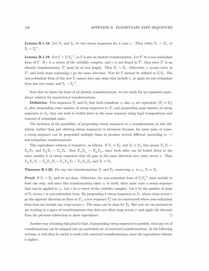
138 APPENDIX B. ELEMENTARY STEP SEQUENCES
Lemma B.1.18. Let T1 and T2 be two sweep sequences for a zone z. Then either T1 ∼ T2, or
T1 ∼ T−12 .
Lemma B.1.19. Let T = T1T−12 , so T is also an identity transformation. Let T ′ be a non-redundant
form of T . If v is a vertex of the visibility complex, and v is not found in T ′, then since T ′ is an
identity transformation, T ′ must be of zero length. Then T1 ∼ T2. Otherwise, v occurs twice in
T ′, and both steps containing v go the same direction. Now let T instead be defined as T1T2. The
non-redundant form of this new T cannot have any steps that include v, so again its non-redundant
form has zero steps, and T1 ∼ T−12 .
Now that we know the form of all identity transformations, we are ready for an expanded equiv-
alence relation for unrestricted transformations.
Definition: Two sequences T1 and T2 that both transform z1 into z2 are equivalent (T1 ≈ T2)
if, after prepending some number of sweep sequences to T1 and prepending some number of sweep
sequences to T2, they can both be boiled down to the same sequence using legal transpositions and
removal of redundant pairs.
The inclusion of the possibility of prepending sweep sequences to a transformation in this def-
inition (rather than just deleting sweep sequences) is necessary because, for some pairs of zones,
a sweep sequence can be prepended multiple times to produce several different (according to ∼)
non-redundant transformations.
This equivalence relation is transitive, as follows. If T1 ≈ T2, and T2 ≈ T3, this means Ts1T1 ∼Ts2T2, and Ts′2T2 ∼ Ts3T3. Now Ts2Ts′2 ∼ Ts′2Ts2 , since both sides can be boiled down to the
same number k of sweep sequences that all pass in the same direction over some vertex v. Thus
Ts′2Ts1T1 ∼ Ts′2Ts2T2 ∼ Ts2Ts′2T2 ∼ Ts2Ts3T3, and T1 ≈ T3.
Theorem B.1.20. For any two transformations T1 and T2 connecting z1 to z2, T1 ≈ T2.
Proof: If T1 ∼ T2, and we are done. Otherwise, the non-redundant form of T1T−12 must include at
least one step, and since this transformation takes z1 to itself, there must exist a sweep sequence
that can be applied to z1. Let v be a vertex of the visibility complex. Let k be the number of steps
of T1 across v in non-redundant form. By prepending k sweep sequences to T1, whose steps across v
go the opposite direction as those in T1, a new sequence T ′1 can be constructed whose non-redundant
form does not include any steps across v. The same can be done for T2. But now we can pretend we
are working in a space of transformations that does not allow steps across v, and apply the theorem
from the previous subsection to show equivalence. ¤
Another way of stating this proof is that, if prepending sweep sequences is possible, then any set of
transformations can be mapped into an equivalent set of restricted transformations. In the following
sections, it will often be useful to work with restricted transformations, since the equivalence relation
is tighter.
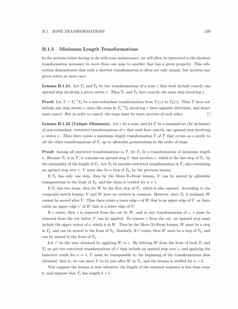
B.1. ZONE TRANSFORMATIONS 139
B.1.5 Minimum Length Transformations
In the sections below having to do with zone maintenance, we will often be interested in the shortest
transformation necessary to move from one zone to another that has a given property. This sub-
section demonstrates that such a shortest transformation is often not only unique, but involves any
given vertex at most once.
Lemma B.1.21. Let T1 and T2 be two transformations of a zone z that both include exactly one
upward step involving a given vertex v. Then T1 and T2 have exactly the same step involving v.
Proof: Let T ∼ T−11 T2 be a non-redundant transformation from T1(z) to T2(z). Then T does not
include any step across v, since the steps in T−11 T2 involving v have opposite directions, and hence
must cancel. But in order to cancel, the steps must be exact inverses of each other. ¤
Lemma B.1.22 (Unique Minimum). Let z be a zone, and let T be a maximal set (by inclusion)
of non-redundant, restricted transformations of z that each have exactly one upward step involving
a vertex v. Then there exists a minimum length transformation T of T that occurs as a prefix to
all the other transformations of T , up to allowable permutations in the order of steps.
Proof: Among all restricted transformations in T , let T1 be a transformation of minimum length
n. Because T1 is in T , it contains an upward step V that involves v, which is the last step of T1, by
the minimality of the length of T1. Let T2 be another restricted transformation in T , also containing
an upward step over v. V must also be a step of T2, by the previous lemma.
If T1 has only one step, then by the Move-To-Front lemma, V can be moved by allowable
transpositions to the front of T2, and the claim is verified for n = 1.
If T1 has two steps, then let W be the first step of T1, which is also upward. According to the
composite match lemma, V and W have no vertices in common. However, since T1 is minimal, W
cannot be moved after V . Thus there exists a lower edge e of W that is an upper edge of V , or there
exists an upper edge e′ of W that is a lower edge of V .
If e exists, then e is removed from the cut by W , and in any transformation of z, e must be
removed from the cut before V can be applied. To remove e from the cut, an upward step must
include the upper vertex of e, which is in W . Thus by the Move-To-Front lemma, W must be a step
in T2, and can be moved to the front of T2. Similarly, if e′ exists, then W must be a step of T2, and
can be moved to the front of T2.
Let z′ be the zone obtained by applying W to z. By deleting W from the front of both T1 and
T2 we get two restricted transformations of z′ that include an upward step over v, and applying the
inductive result for n = 1, V must be transposable to the beginning of the transformations thus
obtained: that is, we can move V to be just after W in T2, and the lemma is verified for n = 2.
Now suppose the lemma is true whenever the length of the minimal sequence is less than some
k, and suppose that T1 has length k + 1.

140 APPENDIX B. ELEMENTARY STEP SEQUENCES
Let Tcross ∼ T−11 T2 be a non-redundant transformation from T1(z) to T2(z), which obviously
satisfies the same restriction on vertices. If Tcross does not have any steps in common with T−11 , then
the lemma is verified, as follows: Let Tboth = T1Tcross, so Tboth connects z to T2(z). If Tcross does
not have any steps in common with T−11 , this is another way of saying that there are no redundant
pairs that can be formed in Tboth. That is, since T2 ∼ Tboth, Tboth is an allowable permutation of
the steps of T2, and so T1 can be considered to be a prefix of T2.
From now on, suppose Tcross does have a step W in common with T−11 . Suppose W is the i-th
step of Tcross and the j-th step of T−11 . Let us define the shared index of W to be the lesser of i and
j. This shared index may change based on various equivalent orderings of the steps of Tcross and
T−11 , however, so let us define the minimum shared index of W to be the minimum possible shared
index of W , over all allowable orderings of the steps of Tcross and T1 (those which can be obtained
by allowable transpositions). Finally, of all the steps that Tcross and T−11 have in common, let W0
be a step whose minimum shared index l is no larger than that of any other shared step. WLOG,
we assume that the steps of Tcross and T−11 are ordered in such a way that W0 is as close to the
front of each sequence as possible.
The size of l is bounded by the length of T1, namely l ≤ k + 1. For the moment, assume that
l ≤ k.
The vertices of W0 are not included in any of the steps of Tcross or T−11 leading up to W0, as
follows. Suppose otherwise, so for example there is a step W1 of Tcross that includes a vertex vshared
which is also found in W0. Now the transformation Tboth = T1Tcross can be reduced so that the
first instance of vshared in Tcross is canceled out by the inverse step in T1. Thus T1 must contain
the inverse of W1, before the inverse of W0. But then we have identified a step in common between
Tcross and T−11 , whose minimum shared index is less than l. So there cannot be a step W1 before
W0 in Tcross that shares a vertex with W0. The same conclusion holds for T−11 .
Suppose WLOG that W0 is an upward step. Let Tmin be the minimum length transformation
(with the same restriction as T1) from T1(z) that includes an upward step over some vertex v0 of
W0. According to the inductive hypothesis, Tmin is unique, and can be found as a prefix, up to
order, of all other restricted transformations from T1(z) that include an upward step over v0. We
have assumed that it is not possible to re-order T−11 so that W0 is closer to the front, so Tmin must
include the steps of T−11 before W0. In particular, Tmin includes the first step of T−1
1 , which is the
inverse of V .
Now however, Tmin also must occur as a prefix to Tcross, up to allowable orderings of the steps
of Tcross. This means that the step involving v of Tmin must also be present in Tcross. However,
this contradicts the fact that this step must have been canceled between T1 and T2 when Tcross was
reduced to non-redundant form. Thus in this case it is impossible for Tcross to have had a shared
step with T−11 , and so once again Tboth must be non-redundant, so T1 occurs as a prefix, up to order,
of T2.

B.1. ZONE TRANSFORMATIONS 141
What if l = k + 1? The length of Tcross must be at least l, i.e. the length of Tcross would be
at least k + 1. Also, there could only be one shared step between Tcross and T−11 , since otherwise
any ordering of T−11 would have a shared step of index ≤ k. If Tcross and T−1
1 have only a single
step in common, then returning to Tboth = T1Tcross, this means that there is only one possible
cancelation when boiling Tboth down to non-redundant form. Thus the non-redundant form of Tboth
will have length equal to two less than the sum of the lengths of Tcross and T−11 , which is at least
(k + 1) + (k + 1)− 2 = 2k. The non-redundant form of Tboth has the same length as T2, so T2 would
then have length at least 2k. For the cases of interest, k ≥ 2. Thus T2 must have length greater
than T1.
If T2 has length greater than T1 in all cases where l = k + 1, then for all T2 of the same length
as T1, by the above reasoning we have that T1 must occur as a prefix, up to order, of T2. Thus the
steps of T1, for n = k + 1, are unique. The reason we originally required l to be ≤ k was precisely
to be able to verify this fact when looking at Tmin. Now we no longer need l to be less than k, and
so the inductive step is complete. ¤
The minimum length transformation T described above has several interesting properties, in-
cluding the following: if T includes a step over a vertex w, then there is no other step of T over
w. In order to prove this property, it is helpful to be able to distinguish between the occurrences of
a given vertex in the steps of a transformation. For any given transformation T = V1, V2, ..., Vn, a
vertex w appearing in a step Vi will be called a new vertex if it is the first time that w has appeared
in any of the steps V1, V2, ..., Vi, and it will be called old otherwise.
Lemma B.1.23 (Second Decomposition). Let T be any non-redundant transformation. Then
the order of steps of T can be rearranged (by allowable transpositions) so that T = TnewTold, the
concatenation of a subsequence containing only steps across new vertices, and a subsequence with
steps containing only old vertices.
Proof: First decompose T into TupTdown, the concatenation of two unidirectional sequences. Note
that the designation of “new” vertices is unaffected by this rearrangement, since by non-redundancy
none of the vertices appearing in steps of Tup appear in any of the steps of Tdown.
Second, let us focus on Tup, pretending that it is the whole sequence. We would like to move all
the steps composed of new vertices to the front of Tup.
We first show that both new and old vertices are never found in a single step. Let Vi be a
composite step of Tup that includes both a new and an old vertex. Then there is an ascending
chain of interior edges from the old vertex to the new vertex, along which must be an edge e whose
lower vertex v1 is an old vertex, and whose upper vertex v2 is a new vertex. In any previous step
containing v1, e must be an upper edge, since v2 must not be part of it. Also, since all the previous
steps are upward, such a step must add e to the cut. No other previous steps can affect e at all,
since they also do not include v2. But e cannot be in the cut just before Vi, since e is an interior

142 APPENDIX B. ELEMENTARY STEP SEQUENCES
edge of Vi. This contradiction shows that we cannot have a composite step with both new and old
vertices in Tup.
Suppose some step Vi has only old vertices, and Vi+1 has only new vertices. If there is no such
pair, then all the steps of new vertices are already at the front of Tup. Suppose there is an upper
edge e of Vi that is also a lower edge of Vi+1. Let v1 be the lower vertex of e, which is in Vi and
thus is an old vertex. Let v2 be the upper vertex of e, which is in Vi+1 and thus is a new vertex.
As in the previous paragraph, this leads to a contradiction, since e must be in the cut just prior to
Vi. Suppose instead that e is a lower edge of Vi and an upper edge of Vi+1, so that v1 is now a new
vertex and v2 is an old vertex. Then e must have been a lower edge before, so it could not be in the
cut just prior to Vi, resulting in a contradiction. So as in the transposition lemma, this argument
shows that the incident edges of Vi and Vi+1 are completely independent, and so Vi and Vi+1 can
be transposed.
Thus by repeated transpositions, all the steps composed of new vertices can be moved to the
front of Tup.
Third, apply the same process to Tdown. Again, due to non-redundancy, no vertex that appears
in Tup can appear in Tdown, so the designation of “new” vertices is unaffected by the fact that we
are focusing on a second part of T .
Fourth, move the steps of Tup that are composed of old vertices to the end of T . Thus all the
new vertices, in both Tup and Tdown, are now at the front of the sequence. ¤
Now we can apply this second decomposition to minimum length transformations:
Lemma B.1.24 (Single Crossing). Let T be the minimum length restricted transformation from
a zone z that includes an upward step across a given vertex v. Then T is unidirectional, and for any
vertex w of the visibility complex, T includes at most one step across w.
Proof: The upward step of T that includes v must be the last step Vlast of T , otherwise T would not
be of minimum length. Because the steps of T could be rearranged to have all the downward steps
at the end, T must be unidirectional. Again, because the steps of T could be rearranged to have all
the steps with new vertices at the front, and since Vlast must be a step containing new vertices (it
must be the only step containing v), T must be composed solely of steps of new vertices. ¤
B.2 Motion and Zone Connectivity
The first section claimed that, in addition to being good sweep structures, zones are also well suited
to incremental maintenance when objects of the scene are allowed to move. In order to examine how
a zone can be maintained, this section studies the effects of continuous object movement on a space
of connected zones.

B.2. MOTION AND ZONE CONNECTIVITY 143
The connections between zones can be restricted by barring steps across a given set of vertices,
and they can also be restricted in another way: by only allowing transformations that are composed
of elementary steps. These elementary transformations will be seen to be simpler from an
algorithmic point of view than the general case. Note that the results and tools of the previous
section apply to elementary transformations as well as general transformations, since it was never
assumed that a given step had to be a composite step.
The effects of motion on a space of connected zones depends on the precise relationship between
the combinatorial changes in the visibility complex, and particular zones or step sequences. The first
subsection below describes the effect of continuous motion on the visibility complex as a whole. The
next two subsections examine combinatorial changes that preserve cut edges, assuming elementary
or general transformations, respectively. The next subsection considers combinatorial changes that
destroy cut edges, and the final subsection describes the role of changes in the set of restricted
vertices.
B.2.1 Definition of Triple Events
When the objects of a scene begin to move, no change in the combinatorial structure of the visibility
complex occurs until a single maximal segment becomes tangent to three objects at once. The
instantaneous formation and disappearance of such a triple tangent is called a triple event. In this
section, we assume non-degeneracy in both the static configuration (no triple tangents not caused
by triple events) and in the motion (triple events are always separated in time).
vb
va
vc
va
vc’
’
e1 e2
e3
eac
e4e5
e6
eab
ebc
e3 e2
e1
eac
e4
e6e5
’
e3e2e1
e4 e5e6
Figure B.1. a triple event
As can be verified by lining up three glasses on a table, a triple event involves either the creation
or destruction of a face of the visibility complex. When a face f is about to disappear, it has three
vertices along its boundary, and three edges. Let va, vb, and vc be these three vertices, ordered by
locally consistent angles for f , so that va has the greatest angle/height, then vb, then vc. Let eab be
the edge between va and vb, let ebc be the edge between vb and vc, and let eac be the edge between
va and vc (see Fig. 2).
In the disappearance of f , va, vb, and vc become momentarily collinear, and then are replaced

144 APPENDIX B. ELEMENTARY STEP SEQUENCES
by two new vertices v′a and v′c, with v′a above v′c, connected by a single edge e′ac.
The other six edges connecting to va, vb, and vc remain intact, as follows. Let e1 and e2 be
the edges above va, let e3 6= eab be the other edge above vb, let e4 and e5 be the edges below vc,
and let e6 6= ebc be the other edge below vb. After the triple event, among the edges above, e3 and
e1 connect to v′a, and e2 connects to v′c. Among the edges below, e4 and e6 connect to v′c, and e5
connects to v′a.
Basically, at the time of the triple event, a degenerate vertex is formed, with three edges above
and three edges below, which are then divided up among the non-degenerate vertices that appear
afterward. Note that the triple event is signaled by one or three edges shrinking together, depending
on whether a face is appearing or disappearing.
For the rest of this section, let C be the visibility complex for a scene of objects at a particular
point in time, and let C ′ be another visibility complex for the same scene at a later point in time,
such that the only (combinatorial) difference between C and C ′ is due to a single triple event. We
indicate the analogue of a zone z of C in C ′ as z′, where it is defined by using the same cut edges.
B.2.2 Triple Events and Elementary Transformations
When two zones are connected in C, if neither zone is affected by a triple event, then we would like
to say that their analogues will also be connected in C ′. We show that this is indeed the case for
elementary transformations, if the following condition is satisfied:
Acyclicity Condition: A nonredundant elementary transformation T satisfies the acyclicity
condition if, for any pair of elementary steps vi and vj of T whose vertices are found at the opposite
ends of a disappearing edge e (disappearing due to a triple event), the order of elementary steps of
T can be permuted so that vi and vj are adjacent in the new ordering.
Two zones connected by an elementary transformation that meets the acyclicity condition are
said to also satisfy this condition. A step of an elementary transformation will be represented directly
as a vertex, rather than a set containing that vertex.
Lemma B.2.1 (Elementary Connectivity). If z1 and z2 are two connected zones in C that
satisfy the acyclicity condition, and the triple event from C to C ′ does not remove any of their cut
edges, then z′1 and z′2 are also connected by an elementary transformation in C ′.
Proof: Let T be a non-redundant elementary transformation from z1 to z2 that satisfies the acyclic-
ity condition. There are two cases, corresponding to the two types of triple events. The first case
examines a triple event where a face disappears, and this case does not make use of the acyclicity
condition. The second case examines the creation of a new face. In both cases we use the variables
defined in the previous subsection to describe the triple event.
Case 1: va, vb, and vc join together. If T does not include any of va, vb, or vc, then the lemma is
satisfied, since the very same sequence of elementary steps can be used to connect z′1 and z′2 in C ′.

B.2. MOTION AND ZONE CONNECTIVITY 145
Let us assume otherwise. According to the hypothesis, z1 and z2 are unchanged by the triple event,
so edges eab, ebc, and eac cannot be cut edges of either zone.
Thus, if va, vb, or vc occur in the sequence T = v1, v2, ..., vn, the first such occurrence must be
a step down across va, or a step up across vc. Without loss of generality, assume it is a step down
across va at vi. When this occurs, eab will be in the zone thus formed. In order for eab not to be in
z2, there must be a step down over vb later in the sequence. (There cannot be a step up over va, by
non-redundancy.)
Let vj be the next elementary step down over vb. Now because neither va nor vb is visited
between vi and vj , eab remains in the zone for that entire subsequence. Also, while eab is a cut edge,
f is a zone face, so eac must also be part of all the cuts constructed between vi and vj . Therefore,
the edges eab and eac are not needed by any of the elementary steps between vi and vj . Thus we
can modify the sequence T to postpone vi until immediately before vj .
Let vk be the first time that vc is an elementary step vertex after vj . Following a similar argument,
vk can be repositioned back in the sequence to just after vj . Thus T can be transformed into an
equivalent sequence, but with the first occurrence of va, vb, and vc precisely in a consecutive triplet
of all three.
Given a consecutive triplet of elementary steps across va, vb, and vc in C, we can obtain the
same effect in C ′ by replacing the triplet with a doublet of the new vertices v′a and v′c that appear
in C ′. This is because, just prior to the triplet, we must have the edges e1, e2, and e3 in the zone,
and the effect after the triplet is to replace these with e4, e5, and e6. A pair of events with v′a and
v′c in C ′ has exactly the same precondition, and exactly the same result. Thus any such triplet of
elementary steps can be transcribed into C ′ to be used in connecting z′1 and z′2.
Case 2: The triple event goes the other way, so that an edge disappears and a new face f appears.
We use the same notation as before, but with the understanding that va, vb, and vc now belong to
C ′, and v′a and v′c belong to C. This time, however, we invoke the acyclicity condition in order to
reposition an occurrence of v′a next to an occurrence of v′c in T .
With similar reasoning as in Case 1, this doublet of elementary steps in C can be transposed
into a triplet of elementary steps in C ′.
Finally, since one occurrence of vertices involved in a triple event is not a barrier to translating
T into an equivalent sequence in C ′, neither is a finite set of them, since they can be converted one
by one. Therefore z′1 and z′2 are connected in C ′ by another transformation T ′. ¤
In other words, provided that cut edges are not involved in triple events and the acyclicity
condition can be met, the connectedness property of two zones is invariant under the motion of scene
objects. Note also that if the elementary transformations are restricted with respect to vertices, as
long as restricted vertices are not involved in triple events, the corresponding transformations in C ′
are also allowed under the restriction.
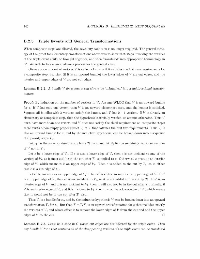
146 APPENDIX B. ELEMENTARY STEP SEQUENCES
B.2.3 Triple Events and General Transformations
When composite steps are allowed, the acyclicity condition is no longer required. The general strat-
egy of the proof for elementary transformations above was to show that steps involving the vertices
of the triple event could be brought together, and then ‘translated’ into appropriate terminology in
C ′. We seek to follow an analogous process for the general case.
Given a zone z, a set of vertices V is called a bundle if it satisfies the first two requirements for
a composite step, i.e. that (if it is an upward bundle) the lower edges of V are cut edges, and the
interior and upper edges of V are not cut edges.
Lemma B.2.2. A bundle V for a zone z can always be ‘unbundled’ into a unidirectional transfor-
mation.
Proof: By induction on the number of vertices in V . Assume WLOG that V is an upward bundle
for z. If V has only one vertex, then V is an upward elementary step, and the lemma is satisfied.
Suppose all bundles with k vertices satisfy the lemma, and V has k + 1 vertices. If V is already an
elementary or composite step, then the hypothesis is trivially verified, so assume otherwise. Thus V
must have more than one vertex, and V does not satisfy the third requirement on composite steps:
there exists a non-empty proper subset V1 of V that satisfies the first two requirements. Thus V1 is
also an upward bundle for z, and by the inductive hypothesis, can be broken down into a sequence
of (upward) steps T1.
Let z1 be the zone obtained by applying T1 to z, and let V2 be the remaining vertex or vertices
of V not in V1.
Let e be a lower edge of V2. If e is also a lower edge of V , then e is not incident to any of the
vertices of V1, so it must still be in the cut after T1 is applied to z. Otherwise, e must be an interior
edge of V , which means it is an upper edge of V1. Then e is added to the cut by T1, so in either
case e is a cut edge of z1.
Let e′ be an interior or upper edge of V2. Then e′ is either an interior or upper edge of V . If e′
is an upper edge of V , then e′ is not incident to V1, so it is not added to the cut by T1. If e′ is an
interior edge of V , and it is not incident to V1, then it will also not be in the cut after T1. Finally, if
e′ is an interior edge of V , and it is incident to V1, then it must be a lower edge of V1, which means
that it would not be in the cut after T1 also.
Thus V2 is a bundle for z1, and by the inductive hypothesis V2 can be broken down into an upward
transformation T2 for z1. But then T = T1T2 is an upward transformation for z that includes exactly
the vertices of V , and whose effect is to remove the lower edges of V from the cut and add the upper
edges of V to the cut. ¤
Lemma B.2.3. Let z be a zone in C whose cut edges are not affected by the triple event. Then
any bundle V for z that contains all of the disappearing vertices of the triple event can be translated

B.2. MOTION AND ZONE CONNECTIVITY 147
into an equivalent bundle V ′ for z′ in C ′ (in the sense that the effect on the cut of the associated
transformations are the same).
Proof: Let V ′ be the bundle obtained by replacing the disappearing vertices of the triple event in
V by the newly appearing vertices of the triple event.
The newly appearing edge(s) of the triple event are interior to V ′, since their upper and lower
vertices are in V ′. Because the cut edges of z are not affected by the triple event, the zone z′ has
the same cut edges as z; in particular, z′ does not include the newly appearing edges as cut edges.
Thus the only incident edges of V ′ that are not incident to V are interior edges of V ′, which are not
in the cut z′. Thus V ′ must also be a bundle for z′ in C ′.
The disappearing edge(s) of the triple event are interior to V , since their upper and lower vertices
are in V . Thus the zone zV obtained by applying the unbundled form of V to z also has no cut
edges involved in the triple event. Then the zone zV ′ obtained by applying the unbundled form of
V ′ to z′ must have exactly the same cut edges as zV . ¤
Lemma B.2.4 (General Connectivity). If z1 and z2 are two connected zones in C, and the triple
event from C to C ′ does not remove any of their cut edges, then z′1 and z′2 are also connected in C ′.
Proof: Let T be a non-redundant transformation connecting z1 to z2. As in the elementary transfor-
mation case, let us consider the two types of triple events separately, and use the variables mentioned
before to describe the triple event.
Case 1: A single edge e′ac disappears, as v′a and v′c merge. Let Vi be the first step of T that
contains v′a or v′c. If Vi contains both v′a and v′c, then it is a bundle that contains all the disappearing
vertices of the triple event, and can be translated into another bundle, and thence into a new sequence
of steps, in C ′. So then that part of T can be translated into C ′ without adverse effect.
If Vi contains just one of v′a or v′c, then WLOG suppose it contains just v′a. Then e′ac is a lower
edge of Vi, and since e′ac cannot have been added to the cut before Vi, that means Vi must be a
downward step, which adds e′ac to the cut. Let Vj be the next step after Vi that includes at least
one of v′a or v′c. Vj cannot include both v′a and v′c, since e′ac is a cut edge just prior to Vj , and so
cannot be an interior edge of Vj . There are only two options left, since e′ac must be removed from
the cut by Vj : an upward step that includes v′a, or a downward step that includes v′c. The former of
these is eliminated by non-redundancy, so Vj must contain just v′c.
Now apply allowable transpositions to the sequence T until Vj is as close as possible to Vi in the
order of steps. Note that this re-ordering simply moves steps out from between Vi and Vj , and so
does not affect the relative ordering of the sequence of steps that contain at least one of v′a or v′c.
Let z′ be the zone obtained by applying all the steps of (the re-ordered version of) T prior to Vi to
z. The subsequence of T including all the steps from Vi to Vj is the minimal length transformation
from z′ that includes a downward step over v′c. As a minimal length transformation, it contains at
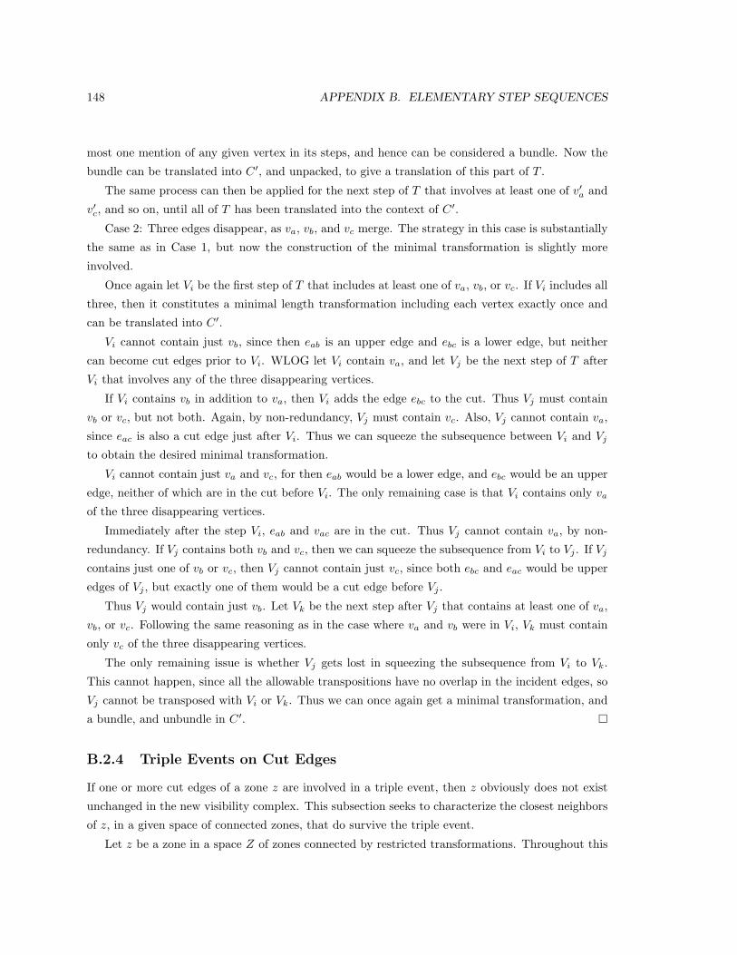
148 APPENDIX B. ELEMENTARY STEP SEQUENCES
most one mention of any given vertex in its steps, and hence can be considered a bundle. Now the
bundle can be translated into C ′, and unpacked, to give a translation of this part of T .
The same process can then be applied for the next step of T that involves at least one of v′a and
v′c, and so on, until all of T has been translated into the context of C ′.
Case 2: Three edges disappear, as va, vb, and vc merge. The strategy in this case is substantially
the same as in Case 1, but now the construction of the minimal transformation is slightly more
involved.
Once again let Vi be the first step of T that includes at least one of va, vb, or vc. If Vi includes all
three, then it constitutes a minimal length transformation including each vertex exactly once and
can be translated into C ′.
Vi cannot contain just vb, since then eab is an upper edge and ebc is a lower edge, but neither
can become cut edges prior to Vi. WLOG let Vi contain va, and let Vj be the next step of T after
Vi that involves any of the three disappearing vertices.
If Vi contains vb in addition to va, then Vi adds the edge ebc to the cut. Thus Vj must contain
vb or vc, but not both. Again, by non-redundancy, Vj must contain vc. Also, Vj cannot contain va,
since eac is also a cut edge just after Vi. Thus we can squeeze the subsequence between Vi and Vj
to obtain the desired minimal transformation.
Vi cannot contain just va and vc, for then eab would be a lower edge, and ebc would be an upper
edge, neither of which are in the cut before Vi. The only remaining case is that Vi contains only va
of the three disappearing vertices.
Immediately after the step Vi, eab and vac are in the cut. Thus Vj cannot contain va, by non-
redundancy. If Vj contains both vb and vc, then we can squeeze the subsequence from Vi to Vj . If Vj
contains just one of vb or vc, then Vj cannot contain just vc, since both ebc and eac would be upper
edges of Vj , but exactly one of them would be a cut edge before Vj .
Thus Vj would contain just vb. Let Vk be the next step after Vj that contains at least one of va,
vb, or vc. Following the same reasoning as in the case where va and vb were in Vi, Vk must contain
only vc of the three disappearing vertices.
The only remaining issue is whether Vj gets lost in squeezing the subsequence from Vi to Vk.
This cannot happen, since all the allowable transpositions have no overlap in the incident edges, so
Vj cannot be transposed with Vi or Vk. Thus we can once again get a minimal transformation, and
a bundle, and unbundle in C ′. ¤
B.2.4 Triple Events on Cut Edges
If one or more cut edges of a zone z are involved in a triple event, then z obviously does not exist
unchanged in the new visibility complex. This subsection seeks to characterize the closest neighbors
of z, in a given space of connected zones, that do survive the triple event.
Let z be a zone in a space Z of zones connected by restricted transformations. Throughout this
B.2. MOTION AND ZONE CONNECTIVITY 149
subsection, a restriction on the vertices of steps will be assumed, but as observed in section 3, this
does not necessarily limit the set of zones under consideration. Let e be a cut edge of z, with upper
and lower vertices vupper and vlower, respectively. Let Ze be the set of zones of Z that do not contain
e as a cut edge. Assume Ze is non-empty (otherwise the entire space of connected zones disappears
after the triple event!)
Lemma B.2.5. Let z′ be an element of Ze, and let T1 and T2 be two non-redundant restricted
transformations connecting z to z′. Then T1 and T2 both have an upward step involving vupper, or
(exclusively) both have a downward step involving vlower.
Proof: T1 must have a step up over vupper or down over vlower in order to remove e from the cut.
T1 cannot have both, by non-redundancy. The same applies to T2. Finally, T1 and T2 connect the
same zones, so T1 ∼ T2. ¤
Thus Ze can be split into two sets: a set Z+e of zones whose (non-redundant) connecting trans-
formations from z contain a step up over vupper, and a set Z−e of the rest, whose connecting trans-
formations from z all contain a step down over vlower. In general, one or the other of these sets may
be empty, for example if z is the maximum or minimum zone of Z. In the following, let us assume
that Z+e is not empty. The same conclusions will apply, with similar reasoning, to Z−e if it is not
empty.
Lemma B.2.6 (Nearest Neighbor). Z+e contains a unique nearest neighbor to z, through which
z is connected to all other zones of Z+e , in the sense that all non-redundant transformations from z
to Z+e can be made to pass through it.
Proof: Let T be any non-redundant restricted transformation from z to any member of Z+e . T can
be written as the concatenation T1T2, where T1 is a non-redundant transformation of z with only
one step down across vlower. Applying the unique minimum lemma to all the possible T1, we obtain
the desired result. ¤
Up until now the edge e has been any cut edge of z. In order to apply these results to triple events,
we also need to consider the case where not just one, but two cut edges simultaneously disappear
in a triple event. A triple event in which two cut edges disappear is an event where an entire zone
face disappears, one of whose side chains contains only one edge. By choosing this unique side chain
edge to be e, the zones of Ze described above automatically avoid both disappearing edges, since
they are forced to avoid the entire disappearing zone face.
In summary, if a zone z has at least one cut edge removed by a triple event, then among all the
zones connected to z that are not affected by the triple event, there is a unique nearest neighbor
(if any) above, and a unique nearest neighbor (if any) below, which in turn connect z to all other
possible neighbors.
150 APPENDIX B. ELEMENTARY STEP SEQUENCES
B.2.5 Restricted Vertices
The previous subsection assumed the existence of at least one vertex of the visibility complex that
was not allowed to appear in any transformation, if only to enable a more clear classification of
connectedness relationships. In the applications of zones considered below, however, restricted
vertices are used quite naturally to constrain the set of connected zones under consideration, and
thus to ensure additional properties of the zones. If the objects are allowed to move, however, the
set of restricted vertices must necessarily be allowed to change. This subsection examines the effect
of imposing restricted vertices on a space of connected zones, and in particular the relationships
between one space of connected zones and another that lies on the opposite side of a restricted
vertex.
Lemma B.2.7. Let Z be a space of zones connected by restricted transformations that are not
restricted with regard to some vertex v. If v is added as a restricted vertex, then Z is split into k+1
connected components, where k is the maximum number of times v appears in any non-redundant
transformation connecting one element of Z to another.
Proof: Let T = V1, V2, ..., Vn be a non-redundant transformation, connecting za to zb in Z, such
that it contains k steps across v. Let z1, z2, ...zk be the zones encountered along T immediately after
each of the steps across v, and let z0 = za. We seek to show that the zi are drawn from each of k +1
connected components.
Let z′ be any zone of Z. Let T ′ be a non-redundant restricted transformation connecting za to
z′, and let l ≤ k be the number of times that v appears in T ′. Let Tl be the prefix of T ending with
the l-th step across v, so that zl = Tl(z0). Let Tcross be a non-redundant transformation connecting
zl to z′. Thus T ′ ∼ TlTcross. These three transformations are non-redundant, meaning that all the
steps in one such transformation across v are in the same direction. Because the aggregate number
of steps across v in a particular direction must be the same on both sides of the ∼ sign (after removal
of redundancies), the number of steps across v in Tcross must be either zero or 2l.
If the number of steps across v in Tcross is 2l, then this means the direction of the steps across v in
T ′ is opposite to those in T . Then T−1T ′ is a transformation from zb to z′, which in non-redundant
form has k + l steps across v. Then l Would be zero, since k is already maximal.
In either case, the number of steps of Tcross across v must be zero. Thus all zones of Z are
connected by non-redundant transformations that do not cross v to one of z0, ..., zk, and two zones
so connected to a particular zl are obviously still connected when the restriction on v is applied. ¤
The proof of the above lemma also implied that if Zi and Zj are two of the connected components
resulting from adding v to the set of restricted vertices, then all non-redundant transformations from
elements of Zi to elements of Zj have the same number n (and same direction) of steps across v.
Conversely, all non-redundant restricted transformations from Zi that include exactly n steps in the
required direction across v land in Zj . Suppose Zi and Zj are neighboring components, in the sense

B.3. ZONE MAINTENANCE ALGORITHMS 151
that n is one. As in the previous subsection, we would like to know if there is a nearest neighbor to
a zone z of Zi in Zj .
Lemma B.2.8. Let z be a zone in a space of zones Zi connected by restricted transformations,
where v is a restricted vertex. Let Zj be another space of connected zones with the same restriction,
which can be reached by transformations having a single step up across v from Zi. Then z has a
unique nearest neighbor in Zj , which can be reached by a unidirectional transformation.
Proof: Application of the unique minimum lemma. ¤
Note that the choice of an upward step in the above lemmata was arbitrary; it could just as
well have been a downward step. In summary, this section has described a basic set of properties
of connected spaces of zones. These properties can be now be applied to the construction of zone
maintenance algorithms.
B.3 Zone Maintenance Algorithms
We now have the tools to describe general algorithms for maintaining a zone as objects move. The
first subsection below treats the case where only elementary transformations are allowed, and thus
can only be applied when the acyclicity condition is satisfied. The section subsection gives the
general algorithm for transformations that can include composite steps.
B.3.1 Elementary Transformations
Given a zone z, we would like to maintain z as objects move. First, we need to detect and handle
events where a cut edge of z disappears. Second, we need to detect and handle changes in the
set of restricted vertices, which may include moving z to the other side of a restricted vertex. In
order to accomplish these operations with elementary transformations, we must make the following
assumptions about the space of zones Z within which z is maintained:
Assumption 1: The space of zones Z never entirely collapses due to object motion.
Assumption 2: The connecting transformations in Z, or at least the elementary transformations
used in maintaining z, satisfy the acyclicity condition.
Also, there must be a representation for the zone that can be updated to reflect an elementary
step, and that contains the following combinatorial information:
• the cut edges and their local combinatorial structure, including their upper and lower vertices.
• local relationships between cut edges: when two cut edges lie on a single zone face, or alter-
natively when two cut edges have the same tangent object.
• the restricted vertices.

152 APPENDIX B. ELEMENTARY STEP SEQUENCES
• for each restricted vertex vr, a corresponding cut edge connected to vr via an ascending or
descending chain of non-cut edges.
Finally, the representation of the zone and the representation of motion must together allow
detection of the collapse of cut edges, and any desired changes in the set of restricted vertices or
their position with respect to the zone.
The reasons for specifying the characteristics of a desirable representation, rather then actually
describing one, is that this representation may vary depending on the problem being solved, and
may also require lengthy justification. In this paper, we simply claim that such representations exist.
Zone Maintenance Algorithm: The two events to be handled are the disappearance of a cut
edge, or movement to the other side of a restricted vertex. In the latter event, let vr be the restricted
vertex. Let e be a cut edge connected to vr by an ascending (or descending) chain of edges, and
let v be the upper (resp. lower) vertex of e. Let Move-Across be the algorithm described below
for moving the zone to the other side of a cut edge vertex. After applying Move-Across to v, check
whether the zone has been moved to the other side of vr. If not, repeat this process of identifying
a vertex on a connecting chain from a cut edge to vr, and moving the zone across it, until the zone
is found to be on the other side of vr. In the former event where a cut edge e disappears, let v be
the upper or lower vertex of e. Apply the Move-Across algorithm to v, and if there is no feasible
transformation across v, apply the Move-Across algorithm to the opposite vertex of e.
For efficiency reasons, when handling the collapse of a cut edge, it may be helpful to have an
oracle that indicates a vertex of the disappearing cut edge which is guaranteed to have an associated
feasible transformation, but as far as correctness is concerned, this is not necessary.
Move-Across Algorithm: Given a vertex v which is the upper (or lower) vertex of the cut
edge e, we would like to move z to the other side of v. There are two basic approaches, depending
on the zone representation:
Case 1: The zone representation allows us to obtain the cut edge on the opposite side chain of
an incident face of a given cut edge. In particular, let e1 be the cut edge on the opposite side chain
from e on the zone face whose maximal (resp. minimal) vertex is v. Suppose e1 not incident to v,
so the edge other than e below (resp. above) v is not a cut edge. Let v1 be the upper (resp. lower)
vertex of e1. Recursively apply the Move-Across algorithm to v1, and then to the next vertex just
above (resp. below) the cut along the opposite side chain from e, until the other edge incident to v
is a cut edge. Finally, apply an elementary step across v.
Case 2: The zone representation (more easily) allows us to obtain the cut edges tangent to a
given object. Let A be the tangent object of v that is not tangent to the maximal segments of e.
Let e1 be the cut edge tangent to A that is nearest v, in the sense that if v is the upper vertex of e,
then e1 is connected with an ascending chain of non-cut edges to v. Now as in Case 1, if e1 is not
incident to v, recursively apply the algorithm until the other edge below v is in the cut, and apply
an elementary step to v.
B.3. ZONE MAINTENANCE ALGORITHMS 153
In either case, if v is a restricted vertex, return failure, or if a cut edge ek is encountered twice,
return failure.
The correctness of the overall algorithm depends on the correctness of the Move-Across algorithm,
so we examine this first.
Lemma B.3.1 (Move-Across). If v is an incident vertex to a cut edge of z, and there exists
a restricted elementary transformation of z that steps across v, then the Move-Across Algorithm
applied to v identifies and applies the shortest possible such transformation. If not, the Move-Across
algorithm fails, leaving a zone connected to z by a restricted elementary transformation.
Proof: (Sketch) If there is no connecting transformation from z to the other side of v, then Move-
Across will return failure, since Move-Across only applies elementary steps (across unrestricted
vertices) in one direction, and hence must run into a restricted vertex or a repeated cut edge at or
before transforming z into the maximal (or resp. minimal) zone.
If there is a connecting transformation from z to the other side of v, let T be the minimal length
transformation. A recursive invariant is as follows: for any recursive invocation of Move-Across, the
input vertex v has a corresponding elementary step in T . This ensures that no restricted vertices are
encountered. Also, if during the recursion a cut edge f is encountered twice, then it can be shown
that there is a cycle of non-cut edges that needs to be crossed, resulting in a contradiction. Thus
the algorithm must terminate with a step across v, and by the recursive invariant the only steps
applied correspond to an application of the transformation T . ¤
Proof: If there is no connecting transformation from z to the other side of v, then Move-Across
will return failure, since Move-Across only applies elementary steps (across unrestricted vertices)
in one direction, and hence must run into a restricted vertex or a repeated cut edge at or before
transforming z into the maximal (or resp. minimal) zone.
Suppose then that there does exist a connecting transformation from z to a zone on the other side
of v. According to the minimum length lemma, there exists a unique minimum length transformation
T (up to ordering) that accomplishes this task. We claim that the Move-Across algorithm identifies
and applies the transformation T .
In order for the zone z to move across the vertex v, by definition an upward elementary step across
v must eventually be applied, and so this elementary step must be the last step of T . Assume WLOG
that T is upward. A recursive invariant is as follows: for any recursive invocation of Move-Across,
the input vertex v has a corresponding upward elementary step in T .
If the input vertex v has two incident cut edges, then the recursion stops, and the invariant does
not need to be verified any further. Otherwise, in both Case 1 and Case 2, an upward chain of
non-cut edges exists connecting e1 to v. Let e′ be the other edge below v other than e, and let v2
be the lower vertex of e′. Because T is a unidirectional transformation, the only way that e′ can be
added to the cut is if there is an upward step across v2. One of the edges below v2, say e2, is on

154 APPENDIX B. ELEMENTARY STEP SEQUENCES
the chain of non-cut edges from e1 to v, and in order for there to be an upward step across v2, e2
must at some point be added to the cut. Continuing down the chain, it therefore must be the case
that the upper vertex of e1 is the vertex of an upward elementary step of T . Thus this recursive
invariant must be satisfied, one result of which is that a restricted vertex will never be encountered.
Now suppose that, during the recursion, a cut edge f is encountered for the second time. Let vf
be the upper vertex of f .
If vf had both lower edges in the cut the first time it was encountered, then an elementary step
was applied to vf . From the single crossing lemma, we know that there is at most one elementary
step across vf in T , so once this step was applied, there would no longer be a step across vf in T ,
and thus there could not be any further recursive calls with input vf . But that we would mean that
f was not encountered again, a contradiction. Therefore vf cannot have had both lower edges in
the cut the first time it was encountered.
Instead, when Move-Across was first applied to vf , there existed an upward chain of non-cut
edges connecting some other cut edge vertex v1 to vf . When Move-Across was applied to v1, if
that recursion terminated before vf , another vertex v2 was identified that also was connected to
vf though an ascending chain of non-cut edges. Let w1 be the vertex in the series v1, v2, ... whose
recursive call to Move-Across did not terminate, since it eventually reached vf . Of all the recursive
calls spawned by w1, one did not terminate, and let w2 be the vertex responsible. Again, w2 is
connected to w1 with an ascending chain of non-cut edges. Continuing in this manner, a sequence
of vertices w1, w2, ... is identified that eventually reaches vf . In the course of this construction, we
find that vf is connected to itself by an ascending chain of non-cut edges.
Now however this shows that there cannot be an elementary step transformation from z with an
upward step over vf , since in order to have a step across vf , both edges below vf must be added to
the cut, and in order for one of the edges of this upward chain to be added to the cut, at least one
other of the edges of the chain must also be added to the cut. Thus the initial hypothesis that a
given cut edge f was encountered twice must be false.
Now that any cut edge is encountered at most once, any given recursion must terminate by
finding a valid elementary step. Each elementary step so found is an elementary step of T , so the
top level recursion, including all the elementary steps, must also terminate. Furthermore, since any
edge is encountered at most once, the total number of calls to Move-Across is exactly the number
of elementary steps of T . ¤
Theorem B.3.2. The Zone Maintenance Algorithm correctly maintains a zone z under motion of
scene objects, given the preceding assumptions 1 and 2.
Proof: When the zone z needs to be moved to the other side of a restricted vertex v, we have
assumed that the connected space of allowable zones does not collapse completely, so there exists a
minimal length transformation that will accomplish this task. By identifying a chain non-cut edges
connecting v to a cut edge, just as in the proof of the Move-Across lemma above, all the vertices

B.3. ZONE MAINTENANCE ALGORITHMS 155
of this chain must correspond to elementary steps in this minimal length transformation. Thus,
applying the same reasoning as before, this procedure gradually reveals the elementary steps of the
minimal transformation, until z reaches the other side of v.
When a cut edge e of z collapses, again we have assumed that the connected space of allowable
zones does not disappear entirely, so there exists a zone in either Z+e or Z−e , the connected zones
obtained by upward or downward steps that do not include e. Thus by choosing the right direction,
there is a minimal transformation that removes e from the cut. In the worst case, say that Z+e is
empty, and Move-Across is applied upward. When Move-Across returns failure, the resulting zone
is still in Z, so when Move-Across is then applied in the opposite direction, the appropriate minimal
transformation is applied. ¤
In conclusion, the Elementary Step Algorithm is guaranteed to maintain a zone, assuming the
space Z does not disappear and the acyclicity condition can always be met (when moving across a
restricted vertex). In addition, provided that the direction of updates for collapsing cut edges is cho-
sen correctly, the complexity of updates correspond to the minimum possible length transformations
necessary to allow z to remain a zone.
B.3.2 General Transformations
When transformations that contain composite steps are allowed, the acyclicity condition can be
dropped. However, an additional assumption must be made, namely that the representation is
capable of handling composite steps. A representation that can handle a composite step, however,
can presumably process all the steps necessary to move across an upper vertex of a cut edge (when
the necessary steps exist). Rather than assume a particular representation-dependent procedure for
doing so, we simply assume this procedure, in place of the acyclicity condition:
Assumption 2’: A procedure Move-Across-Bundle exists to move a zone to the opposite
side of a vertex incident to one of its cut edges, provided that such a transformation exists.
Note that a minimal transformation to the other side of such a vertex v involves any vertex of
the visibility complex in at most one step.
The Zone Maintenance Algorithm may now be applied to the general case, simply by using
Move-Across-Bundle in place of Move-Across.
Theorem B.3.3. The Zone Maintenance Algorithm correctly maintains a zone z under motion of
scene objects, given the preceding assumptions 1 and 2’.
Proof: We have already shown that, under the assumption that the space of connected zones
does not disappear entirely, the requisite transformations exist, and that in the minimal length
transformations with no repeated vertices also exist. Thus the only thing left to verify is that, when
Move-Across-Bundle is repeatedly applied vertices found on a chains of non-cut edges to vr, we are
uncovering steps of the minimal transformation across vr.
156 APPENDIX B. ELEMENTARY STEP SEQUENCES
The same reasoning applies as before: assume WLOG that an ascending chain of non-cut edges
connects a vertex v to vr. Then a minimal transformation across vr will eventually have to place the
lower edges of vr into the cut, or else include vr in a composite step that includes the lower edges of
vr as interior edges, or as a mix of an interior edge and a cut edge. Thus we can again traverse this
chain from vr down to v, showing that each edge must at some point be either in the cut, and hence
must there must be a step across its lower vertex, or must have been an interior edge, in which case
the lower vertex must have been part of a composite step, until v itself is reached. ¤
We are now ready to apply the zone transformation algorithm to the zones described in the
introduction, namely zones that capture the lower envelope of a scene, and the zones that capture
the visible set of a moving point observer.
B.4 Lower Envelope Zones
As a first illustration of the results of the last section, let us consider maintenance of the lower
envelope zones defined in the introduction. We will show that it is enough to consider elementary
transformations for this purpose. From previous work, it is known that elementary steps transform
anti-chains into anti-chains, and because the vertical zone is an anti-chain, all lower envelope zones
are anti-chains. The first subsection below shows that anti-chains always satisfy the acyclicity
condition, and the next subsection applies this observation to the problem of maintaining the lower
envelope of a set of (convex, non-overlapping) moving objects.
B.4.1 Acyclicity in Anti-Chains
Anti-chains are defined in the context of maximal segments with angle, where angles differing by 2π
are considered distinct. This consistent assignment of angles implies acyclicity, as follows:
Lemma B.4.1. Let z1 and z2 be two anti-chains connected by a non-redundant elementary trans-
formation T . Then T satisfies the acyclicity condition.
Proof: Suppose otherwise, so that T has a pair of elementary steps vi and vj that cannot be moved
next to each other. That is, there exists a subsequence vi = w0, w1, ..., wk = vj of T where no
transpositions in the order of these steps is possible, and k > 1. This is therefore a unidirectional
sequence, with vertices connected by edges in the visibility complex. Thus the angles of the maximal
segments wi are uniformly increasing from the angle of w0 to the angle of wk. However, for the
acyclicity condition, we also have that vi and vj have a disappearing edge connecting them: the
angular difference between w0 and wk tends to zero as we approach the triple event. Thus there
cannot be any vertices whose angles are between those of vi and vj if the triple event is close
enough. ¤
B.4. LOWER ENVELOPE ZONES 157
B.4.2 Lower Envelope Maintenance
In order to maintain the lower envelope, we simply need to construct and maintain a lower envelope
zone, which contains the requisite information. First, let us define the lower envelope zone more
precisely, using the terminology now available.
A visible face is a face of the visibility complex that contains at least one maximal segment with
infinite extent in the negative y direction. The visible faces thus connect to the lower envelope of
the scene. A visible edge is similarly an edge that contains a maximal segment with infinite extent
in the negative y direction (this maximal segment would be part of the vertical decomposition).
A lower envelope zone is any zone connected to the vertical zone by an elementary transfor-
mation, with the following restriction on vertices: no step can contain a vertex incident to a visible
edge. Thus by restricting the vertices of visible edges, all the lower envelope zones are constrained
to include the visible edges as cut edges, and thus are also constrained to include the visible faces
as zone faces.
To construct an initial lower envelope zone, we construct the vertical zone described in [PV96a]
in O(n log n) time and linear space. Then to maintain the zone, we apply the Zone Maintenance
Algorithm. Note that because any pair of lower envelope zones are connected with a transformation
satisfying the acyclicity condition, we can apply the Zone Maintenance Algorithm for the case of
elementary transformations.
In more detail, maintaining the zone involves two types of events. When a cut edge collapses,
the zone needs to be moved to the other side of one of the incident vertices. The other type of event,
where the zone needs to be moved to the other side of a restricted vertex, also occurs, as follows.
The definition of the visible edges is very similar to that of the lower envelope. When the lower
envelope changes, the set of visible edges changes, and vice versa. These changes occur when two
vertical tangents become aligned, i.e. when a particular vertex v of the visibility complex passes
through a vertical orientation. This vertex v is a restricted vertex both before and after the event–
the difference is that a visible edge has “moved” to the other side of v. Thus to maintain the lower
envelope zone, it is necessary to move the zone to the other side of this restricted vertex. Note that
all restricted vertices are incident to cut edges, so that it is easy to detect when they are about to
pass through a vertical orientation.
This algorithm is thus correct, and depends solely on the maintenance of a single zone. Compared
to maintaining a vertical decomposition, this algorithm behaves ‘lazily’, only updating the zone when
cut edges are destroyed or the lower envelope changes. The cost of this maintenance will depend
on the motion of the objects. In the language of kinetic data structures, the number of certificates
will be proportional to the size of the lower envelope (to detect elementary steps across restricted
vertices) plus the number of moving objects (to detect triple events on cut edges). These zones are
anti-chains, and hence can be represented by pseudo-triangulation data structures, which also serve
as spacial decompositions. As a result, maintaining these zones provides collision detection as well,

158 APPENDIX B. ELEMENTARY STEP SEQUENCES
with no additional overhead. The cost of individual updates depends on the length of the minimal
transformations being computed, and these can vary widely, depending on the history of the motion
of the objects. In the worst case, a single event can trigger a transformation that sweeps though a
large part of the visibility complex. In practice, most of the updates in our test cases can be charged
to collisions, so the cost of maintaining the lower envelope appears almost ‘free’ in comparison.
In summary, this section has described a zone maintenance algorithm for maintaining the lower
envelope of a set of moving objects, while providing collision detection as an intermediate result.
B.5 Visible Zone Maintenance
The visible zones mentioned in section 1 form a second example of zones we would like to be able
maintain in order to preserve some geometric information about the scene. The technical definition
of these zones is entirely analogous to the lower envelope zones: they are the zones connected to the
canonical visible zone by transformations restricted with respect to the upper and lower vertices of
the visible edges (this time to the viewpoint).
Unfortunately the acyclicity condition does not apply in general to visible zones. In the first
subsection below, we present an example where the acyclicity condition fails. In the second subsec-
tion we consider the case where only the observer moves (but not any scene objects), and show that
in this case it is sufficient to use elementary transformations. The third subsection examines the
general case.
B.5.1 Visible Zone Cyclicity
Let S be the scene shown in Figure B.2. The canonical visible zone for this scene is computed from
the radial decomposition (see Figure B.2a). Among all the zones connected by elementary steps
to this canonical visible zone, the zone with the least ‘freedom of movement’ is the maximal zone
obtained by applying a maximal (upward) elementary transformation (see Figure B.2b).
Figure B.2. As the observer moves, two neighboring tangent segments attached to the observer become momentarilycollinear, thus requiring an update to their combinatorial descriptions.
Let A be the smallest object of S, namely the one shaded dark grey. If A is moved down and to
B.5. VISIBLE ZONE MAINTENANCE 159
the left, a triple event occurs that does not affect any of the cut edges, but destroys the elementary
step connection to the canonical visible zone. If A continues this trajectory until the visible set
changes, this update across a restricted vertex cannot be performed using elementary steps.
In addition, the conditions under which acyclicity is violated are not precisely identifiable just
from the combinatorial structure of the zone. In the above example, if the bottom-most object is
moved a little further up, without disturbing the cut edges of z, then the same motion of the small
object can be correctly handled.
B.5.2 Observer Motion
If, however, the objects are static, and only the observer is allowed to move, we once again can rely
on elementary transformations. We seek to establish the invariance of zone connectedness under
observer motions, since that is the only part of the preceding development that depended on the
acyclicity condition. We use the same variables C, C ′ to denote a visibility complex just before and
just after a triple event.
Lemma B.5.1. Let z be a visible zone in C, none of whose cut edges are removed by a triple event
(resulting from observer motion). Then the corresponding zone z′ in C ′ is also a visible zone.
Proof: Let T be a non-redundant restricted transformation connecting z to the canonical visible
zone. The only triple events are those that involve the infinitesimal object around the viewpoint.
These occur either as the viewpoint object reaches a bitangent or an extension of a bitangent. Let
v be the vertex corresponding to the bitangent.
In the latter case, v is a restricted vertex. As a result, T cannot contain any elementary steps
across v, and so can be used unmodified to connect z′ to the canonical visible zone in C ′.
In the former case, although v is not a restricted vertex, it is just above an edge that is in turn
just above a restricted vertex, along a single side chain. If there were an elementary step in T across
such a vertex, then all the adjacent edges would have to be in the cut at some point along the
sequence, but this contradicts the zone definition of just one cut edge along a given side chain. Thus
v cannot be in the sequence T , and T can be used unmodified to connect z′ to the canonical visible
zone. ¤
Thus the remaining tools of section 4 apply to visible zones with observer motion, and the
elementary step algorithm described in section 5 can be applied to these zones correctly.
B.5.3 General Motion
For the general case, it is necessary to handle composite steps. However, in order for composite steps
to really be needed, the transformation T connecting the canonical visible zone to the currently
160 APPENDIX B. ELEMENTARY STEP SEQUENCES
maintained zone z must include composite steps. In order for this to happen, T must not satisfy
the acyclicity condition at some earlier point.
A violation of the acyclicity condition can be shown to involve a cycle of cut edges that links
objects in a circle around the observer. In order for such a cycle to arise, the motion of these objects
must be choreographed in a rather restrictive manner, with the result that, in all our test scenes
with random motions, we were unable to produce any examples of this behavior. Thus it appears
that in many situations the algorithm to handle composite steps would only be used rarely, if at all.
We have found that the algorithm for elementary steps is sufficient for experimentally testing the
behavior of zone maintenance, even when many objects are moving.
Finally, the number of certificates connected to the observer, that is the number of potential
events involving the observer for any given motion, is exactly the number of restricted vertices,
which is in turn proportional to the size of the visible set. Thus when the observer changes its
motion, only these certificates need to be recomputed, in constant time each, for a total cost for
each change in motion proportional to the size of the visible set.
B.6 Amortized Complexity
In this section, the total complexity of the above algorithms will always be expressed in terms of
the number of elementary steps, if elementary transformations are involved, or more generally the
number of vertices involved in the steps of the transformation. We consider just the case of the
visible zones, since maintaining the lower envelope can be considered a special case. Also, note
that all motions are assumed not to involve collisions (including collisions between the viewpoint
and scene objects), since the visibility complex has only been defined for non-overlapping convex
objects.
The first subsection below defines the notion of a wind angle of a maximal segment. The second
section applies wind angles to the movement of cut edges along a given object boundary. The third
sections applies these tools to obtain bounds on the total complexity of updates, given constant
degree polynomial motion. The fourth section defines and analyses the complexity in terms of a
characteristic of a scene called the maximum rigidity.
B.6.1 Wind Angles
An important requirement of this analysis is to somehow account for the history of the motion.
In the original definition of the visibility complex, each maximal segment had an associated angle,
which captured the location of the cut, even when it was raised though a half-turn or a full turn.
We would like to define an analogous quantity, such that if we follow a continuous path of maximal
segments around the perspective point from one maximal segment to itself, this quantity can be
continously propagated from one maximal segment to the next along the path, and still yield the

B.6. AMORTIZED COMPLEXITY 161
same value at the end of such a loop. The difficulty of finding such an assignment has led to the
following definition, which is not so much a single real number as an equivalence class tying angles
and the winding numbers of implicit paths together:
Definition: The wind angle of a maximal segment of a zone face in a visible zone is an angular
difference, between the angle as usually assigned (formed by the supporting line of the maximal
segment with some referent, like the positive x axis), and 2π times an implied winding number of
the maximal segment, with respect to the perspective point.
For example, if we know a priori that segment s has angle π/4 and implied winding number
2, then the wind angle of s would be π/4 − 2 ∗ 2π. If we follow a loop around the perspective
point from s to itself that resembles a rotation, we increase (resp. decrease) the implied winding
number by one, and also increase (resp. decrease) the usual angle by 2π, which taken together does
not change the wind angle. In order to assign wind angles to the maximal segments of (the zone
faces of) a visible zone, we start with a particular maximal segment s0, say the maximal segment
connected to the perspective point whose extension toward infinity is parallel to the positive x axis,
and assign s0 some usual angle, like zero. The other maximal segments of the visible zone can then
be assigned wind angles by connecting them with paths to s0, and continuously propagating wind
angles. Despite the deliberate ambiguity in exactly what value the implied winding number takes
on for paths that do not form loops, the assignment of wind angles can always be performed in a
consistent manner, as follows.
Lemma B.6.1. If a wind angle is assigned to one maximal segment s of a zone face in a visible
zone, then the other maximal segments of the zone face can be assigned wind angles consistent with
s, and which are consistent with each other.
Proof: Let f be a zone face. By definition, f is connected, and contains no maximal segments
passing through the perspective point. Thus it is possible to connect s to each maximal segment
m of f with a path that lies entirely in f , and thereby propagate some wind angle to m. Also, it
is known that each face of the visibility complex is simply connected, at least when there is more
than one object in the scene (we can safely assume). Thus in any path from a segment to itself in
f , the implicit winding number cannot change. Thus the propagation of winding angles is fully as
consistent as propagation of usual angles, and hence is itself consistent within the face. ¤
Lemma B.6.2. When a wind angle is assigned to the maximal segment s0 mentioned above in the
canonical visible zone, then the other maximal segments of the entire zone can be assigned wind
angles consistent with s0, and which are consistent with each other.
Proof: First consider only those maximal segments of zone faces whose supporting lines pass
through the perspective point, and note that s0 belongs to this set R. Then it is clear that the
maximal segments of R can be connected to s0 with paths in R, and that furthermore any path in

162 APPENDIX B. ELEMENTARY STEP SEQUENCES
R from a maximal segment of R to itself will preserve a given wind angle. Also, every zone face
has maximal segments in R. Thus an assignment of wind angles to R can be extended to all the
maximal segments of the zone. Finally, any path p from a maximal segment t of the zone to itself
must then be consistent, as follows.
If p is not consistent, then the inconsistency must appear at the boundary between two zone
faces f1 and f2, since all the subsections of p contained in the interior of any given zone face must
be consistent. Let s be a problematic maximal segment on the boundary between f1 and f2, and
let us assume WLOG that s lies on the interior of an edge of the visibility complex.
Let c be a simple curve in the plane, whose points lie along a segment that coincides with s. Thus
c stretches from the boundary of some object A to the boundary of some object B, and incidentally
is tangent to exactly one object between them. Consider the relationship between c and the cells
of the radial decomposition of the scene. Two of the cells C1 and C2 of the radial decomposition
correspond to f1 and f2, and c may or may not intersect these cells. However, c cannot be too far
from C1 and C2: C1 connects to either A or B, since c must connect to both objects bounding C1.
The same is true for C2. If c does not already intersect C1, then extend c along A or B until it does.
Do the same for c and C2.
Now let s1 be a maximal segment of R that lies in f1, and which also intersects c. Let s2 be
a maximal segment of R that lies in f2, that also intersects c. Let p1 be a path entirely contained
in f1 from s to s1, such that each maximal segment of p1, considered as a set of points in the
plane, intersects with c, and such that a continuous traversal of p1 would imply continuous motion
of this intersection. Let p2 be a path in f2 from s2 back to s, that also continuously maintains an
intersection with c. To each point of c, there is exactly one maximal segment of R that intersects it,
so let p3 be a path in R from s1 to s2, such that all the maximal segments along this path intersect
the curve c, and have this same continuous intersection property. Let p∗ be the path from s to itself
obtained by following p1, then p3, then p2. The winding number of p∗ relative to the perspective
point must be zero, since all the maximal segments of p∗ maintain a continuously moving contact
point with a closed curve in the plane.
This means that, by following this path, the wind angles assigned to s from the side of f1, and
from the side of f2, must be the same. Therefore s cannot have been assigned conflicting wind angles
by the two faces f1 and f2. ¤
Lemma B.6.3. Given two visible zones z1 and z2 connected by a single step V , and a consistent
assignment of wind angles to the maximal segments of z1 can be extended to a consistent assignment
of wind angles in z2.
Proof: (Sketch) In a single elementary step, one zone face is deleted, and one zone face is added.
The new zone face f has the elementary step vertex v on its boundary, whose wind angle can be
used to assign wind angles to all the maximal segments of f . This assignment is consistent within
the new face, by the above lemma on single faces.

B.6. AMORTIZED COMPLEXITY 163
The assignment must also be consistent with all the remaining zone faces, following a similar
path argument as in the previous lemma, as follows. As before, if there is any inconsistency, it must
appear at a boundary maximal segment s between f and some other zone face, g.
The maximal segments of the interior of f are incident to two objects, A and B. Thus s must
also be incident to the boundaries of A and B. Applying the same reasoning to g, and noting that s
is incident to only three objects total, the maximal segments of the interior of g must all be incident
to one of A or B, say A. Thus all the maximal segments of f and g, including s, are incident to the
boundary of A.
It can be shown that, for any two zone faces incident to a given object, there exists a path
connecting them consisting of maximal segments that are always incident to that object, and always
lie in the zone. Thus there is a path p1 from s to v that is always incident to A, and remains in
the ‘old’ zone prior to the elementary step. There exists a second path p2 from v back to s on the
interior of f , which obviously also remains incident to A. Now by putting these two paths together,
we obtain a loop from s to itself, through g then through f , that always remains in contact with
A. This path then cannot involve a change in the implicit winding number, and so there cannot be
any inconsistency at s. An incremental argument along the same lines can be made for composite
steps. ¤
Note that, due to the vertex restriction, no elementary or composite steps can remove the zone
face containing s0 from a visible zone. Thus instead of starting with the canonical visible zone, and
then propagating wind angles to all the connected zones, it is equivalent to always start with s0,
and assign wind angles directly within a given zone.
Thus wind angles can be consistently assigned to all visible zones, and change relatively little as
elementary or composite steps are applied. Because all visible zones can have assigned wind angles,
there is no problem imagining continuously changing wind angles for a visible zone in a moving
context, as well.
Although the exact value of an implicit winding number has deliberately been left fuzzy, it is
nevertheless possible to assign a total order to the wind angles of maximal segments tangent to
a given object A. This is because, given a path of maximal segments which are all tangent to A
that forms a loop, this path has a known winding number, namely zero (assuming A is not the
infinitesimal object around the perspective point). Thus all such wind angles can be compared
purely according to usual angles, by assuming the implicit winding number is relatively fixed. In
particular, relative to this order it makes sense to say that the wind angle is increasing or decreasing
as a maximal segment turns tangent to A.
B.6.2 Representative Maximal Segments
Let e be a cut edge of a visible zone, and let m be a maximal segment of e which is not the upper or
lower vertex. Then m can be considered a representative maximal segment for e, and we can

164 APPENDIX B. ELEMENTARY STEP SEQUENCES
say e has a representative wind angle which is the wind angle of m. In the context of continuous
motion, let us imagine that the representative maximal segment m of e is chosen in such a way that
m varies continuously over time, and that furthermore m moves infinitesimally close to a step vertex
just prior to any steps that will change the zone in the vicinity of e. Note that, in an elementary
step, m can be imagined to move through the step vertex to a new cut edge sharing the same tangent
object A as e, and similarly for a composite step m can be imagined to move through several vertices
to a new cut edge (always remaining tangent to A). Thus even these discrete changes do not affect
the continuity of motion of such a representative maximal segment m, and the continuity of its wind
angle.
If a series of elementary and/or composite steps is applied to the visible zone to transform it into
the canonical visible zone, then m can move in such a way that its supporting line ends up incident
to the viewpoint; this is the canonical position of m. The wind angle of m when m reaches its
canonical position is the canonical wind angle of m.
Lemma B.6.4. Let z be a visible zone, connected by a non-redundant transformation T to the
canonical visible zone, whose first step is V . Let e be a cut edge of z, and suppose e has a particular
representative maximal segment m. When the step V is applied to z, the wind angle of m, if m
changes, is moved closer to its canonical wind angle.
Proof: The wind angle of m must eventually move to its canonical wind angle, if the rest of the
steps of T are applied. By the non-redundancy of T , m must turn in only one direction. ¤
Lemma B.6.5. Let z1 and z2 be two visible zones, just before and just after a change in the
visible set of the perspective point, respectively. Let z2 be obtained from z1 by application of the
transformation T performed by the Zone Maintenance Algorithm. Let e be a cut edge of z1, and
suppose e has a particular representative maximal segment m. When T is applied to z1, the wind
angle of m, if m changes, is moved closer to its canonical wind angle.
Proof: Let T1 be a non-redundant transformation from z1 to its canonical visible zone za. Note
that the canonical zone changes from za to another canonical zone zb during the movement of the
viewpoint across the restricted vertex, and further that this change from za to zb is equivalent to
a simple elementary step across the restricted vertex vr. Let Tr be the transformation consisting
of this elementary step. Then T1Tr is a transformation from z1 to zb, with exactly one step in the
required direction across vr. The transformation T is the minimum length restricted transformation
of z1 that crosses vr, so it occurs as a prefix, up to order, of T1Tr. Also, T must include the same
step across vr as this transformation, at the end. Thus T can be expressed as the concatenation
TpTr, where Tp is a prefix, up to order, of T1.
By applying Tp to z1, m may be forced to move, but if so, according to the previous lemma, m
moves closer to its canonical wind angle. The only remaining question is the effect of Tr on m. If m
is not on one of the cut edges incident to vr, then m is not affected, and we are done.

B.6. AMORTIZED COMPLEXITY 165
If on the other hand m is on one of the cut edges incident to vr, then m is on a cut edge which is
a cut edge of za. That is, m has been brought to such a position that its wind angle can be exactly
the canonical wind angle, prior to the application of Tr. When Tr is applied, all that happens to m is
that m is allowed to continue in its canonical position, so that its wind angle continues to be exactly
the canonical wind angle. Thus if the wind angle of m was changed by Tp, the aggregate change in
the wind angle of m was to bring it closer to the canonical wind angle, and if the wind angle of m
was not affected by Tp, then the wind angle could not have been brought closer to the canonical wind
angle, and continued to be equal to the canonical wind angle as a result of the transformation. ¤
Lemma B.6.6. Let e be a cut edge of a visible zone, and suppose e has a particular representative
maximal segment m. In any update by the Zone Maintenance Algorithm, assuming the direction of
steps is correctly chosen, the wind angle of m, if m changes, is moved closer to its canonical wind
angle.
Proof: Let z be the visible zone, and let T be a non-redundant transformation from z to the
canonical visible zone. The only updates not handled by the previous lemma are those involving the
collapse of at least one cut edge e of z. Suppose WLOG that the canonical visible zone belongs to
Z+e , the set of zones not including e as a cut edge, with an upward step responsible for removing e
from the cut. When the direction of steps is correctly chosen, we apply the minimal transformation
to move z into Z+e . By the unique minimum lemma, this transformation can be found as a prefix, up
to order, of any non-redundant transformation from z to Z+e . In particular, we are applying steps
that form a prefix to T , and so the wind angle of m, if it changes, must move closer to its canonical
wind angle. ¤
Thus intuitively the situation for a single cut edge e that is tangent to an object A can be
described as follows: there is a spring connecting the representative maximal segment of e to its
canonical location. As the viewpoint moves, this canonical location changes, and the spring may
have to lengthen. However, whenever there is an update that affects the cut edge e, this spring is
allowed to pull the representative maximal segment back in. The following subsection applies this
intuition to bound the number of times a given vertex can appear in update transformations, based
on the movement of the perspective point.
B.6.3 Amortized Complexity Analysis
The complexity analysis presented below is only for the case of static objects. When the objects of
the scene are allowed to move, the same bounds will not apply.
Lemma B.6.7. Let z be a visible zone for a static scene and a moving viewpoint, maintained using
the Zone Maintenance Algorithm. Let v be a vertex of the visibility complex, not connected to the
infinitesimal object around the viewpoint. If in the course of a simulation the perspective point

166 APPENDIX B. ELEMENTARY STEP SEQUENCES
crosses the supporting line of v exactly k times, then the update transformations used to maintain
z involve at most 2k steps involving v.
Proof: Let A be one of the objects tangent to v, which is therefore not the infinitesimal object
around the viewpoint. For any canonical zone, A has exactly two cut edges tangent to it, and A
also has two tangent cut edges in any visible zone, since this property is preserved by elementary
and composite steps. Let e1 and e2 be these two cut edges, and let m1 and m2 be representative
maximal segments for them. An update transformation that involves v must therefore cause m1 or
m2 (or both) to pass through the supporting line l of v.
Let us focus on how many times one of the representative maximal segments, say m1, can pass
through l. At the beginning of a simulation, m1 is in its canonical position, and so as long as the
viewpoint stays in one place or moves along the supporting line of m1, m1 cannot be moved by
updates. Once the viewpoint moves off the supporting line of m1, however, the canonical position
changes, and m1 may be forced to move closer to the canonical position.
As long as the viewpoint does not cross l, however, the canonical position of m1 (visualized as
the tangent point corresponding to this position) also does not cross l, and so m1 cannot cross l
either. When the viewpoint finally does cross l, m1 may eventually follow, but if it does, we are
once again in the position that m1 cannot reach l unless the viewpoint leads the way.
In general, then, we can count the number of times the ‘spring’ between m1 and its canonical
position crosses l. Updates that force m1 to move cannot cause this number to increase, and thus
the only way to increase this number is when the canonical position moves across l, i.e. when the
viewpoint crosses l. Also, every update that involves v causes this number to decrease, for at least
one of m1 or m2. Thus the total number of updates across v can be at most 2k. ¤
Theorem B.6.8. Let z be a visible zone for a static scene and a moving viewpoint. If the motion
of the observer can be described with a pseudo-algebraic function of constant degree, then the total
complexity of updates (measured in vertices) is O(k), where k is the number of vertices in the
visibility complex of the static objects.
Proof: The path of the observer, when described by pseudo-algebraic function of constant degree,
crosses the supporting line of any given vertex v (not connected to the observer) a constant number
of times. Therefore, the number of updates involving v is also a constant, which summed over all
such static vertices is proportional to k. As observed in a previous section, maintenance updates
do not involve any vertices that are connected to the infinitesimal object around the perspective
point. ¤

Appendix C
Glossary
above A maximal segment m1 of the visibility complex is ‘above’ another maximal segment m2 if
they belong to the same face and the angle of m1 is greater than the angle of m2 (see also
angle definition).
allowable transposition In a sequence of elementary steps, an allowable transposition is an op-
eration that interchanges the order of two adjacent elementary steps whose effect on the cut
is independent of each other.
angle The angle of a maximal segment m is the angle formed by the supporting line of m with
respect to a fixed referent, such as the x-axis.
approximate visible set The set of objects whose outer bounding boxes intersect the visible re-
gion.
arc bitangent A bitangent that has been flipped, and when it was last flipped, it became part of
a corner arc (at least for awhile).
bitangent width The sector of the field of view of the observer covered by a bitangent, measured in
radians. This measure is independent of whether there are any objects between the bitangent
and the observer or not.
bitangent A line segment tangent at both ends to objects in the scene, whose interior does not
intersect the interior of any scene object, such as those line segments found along a corner arc.
boundary segment A line segment on the boundary of the visibility polygon that connects two
objects.
ClearSeg A procedure by all the bitangents crossing a given boundary segment are flipped, and
thereby no longer intersect the boundary segment.
167

168 APPENDIX C. GLOSSARY
ClearSide A procedure by which one or more bitangents indicent to the forward object of a given
bitangent are flipped, resulting in the construction of the associated corner arc.
coherence boundary The locus of points in space where a particular change in visibility occurs.
collision event When two objects move toward each other and are about to overlap.
connected Two cuts of the visibility complex are connected if there exists a sequence of elementary
steps taking one to the other.
corner arc A topological equivalent to a boundary segment b consisting of a concave chain of
bitangents and connecting object boundary arcs that begins along the tangent object of b and
ends with a bitangent connected to the far object of b.
corner region Given a boundary segment b, the part of the plane enclosed by b, the corner arc of
b, and the far object of b.
cut A set of edges of the visibility complex (called cut edges) with the property that, for any face
of the visibility complex f with a cut edge on its boundary, there is exactly one cut edge on
each of the side chains of f .
deletion event An event in which an SP-object that has been shrunk to a point is removed from
a radial subdivision.
edge In the 2D visibility complex, a maximal connected set of maximal segments each of which has
exactly one tangent point.
elementary step down An elementary step that replaces edges above a vertex with those below.
(see definition for above)
elementary step up An elementary step that replaces edges below a vertex with those above. (see
definition for above)
elementary step 1) An incremental update of the radial subdivision in which two neighboring
tangent segments momentary share the same supporting line, 2) the basic combinatorial update
step for changes to the visible zone, and 3) an operation by which a cut is changed, by removing
two cut edges that share a vertex, and replacing them with the other two edges incident to
the vertex.
endpoint event An event in which the endpoint of the ground query segment moves from one cell
of a radial subdivision to another (or one cell formed by tangent segments of a visible zone to
another).

169
extended ray query A type of ray query where the ray origin lies anywhere in the plane, the
supporting line for the ray passes through the observer, and the query termination criteria
may permit passing through more than one object.
face In 2D, a maximal segment m that is not tangent to any object, whose endpoints lie on some
objects A and B, grouped together with all other maximal segments that can be obtained by
moving the endpoints of m along the boundary of A and B without becoming tangent to any
object in the process.
far object The object indicent to a boundary segment at the endpoint that lies farther, rather than
nearer, to the observer.
far tangent Each tangency event involves two boundary segments only one of which may be present
before or after the event, and the far tangent boundary segment is the boundary segment
whose tangent point is farther from the observer than the tangent point of the other boundary
segment.
flip The basic mechanism for modifying a pseudo-triangulation, in which a bitangent is removed and
replaced with the only other bitangent that can be inserted in the space thus made available.
free space The space surrounding the objects of the scene that is the complement of the union of
their interiors.
ground line The intersection of the sweep plane and the ground plane.
ground plane In a 3d scene, the plane g which all objects in the scene lie above.
ground query segment A line segment in the ground plane (and in the sweep plane) obtained by
projecting the segment s vertically down onto the ground plane, where s is the line segment
joining the point observer to the sky line along a line tangent to the most distant visible object
(s is disjoint from the interior of any object).
insertion event The event when a new SP-object is inserted into a radial subdivision.
interior event An event that occurs during maintenance of the ground query segment in a ra-
dial subdivision (or visible zone) in the ground plane, in which the ground query segment
momentarily contains a tangent segment as a subsegment.
map-object The projection of a 3d object onto the ground plane.
map-observer The projection of the point observer onto the ground plane.
maximal segment A line segment m of free space such that m cannot be lengthened along its
supporting line without intersecting the interior of some object.

170 APPENDIX C. GLOSSARY
maximum cut A cut obtained by applying as many restrictred upward elementary steps as possible
to a given cut.
near tangent Each tangency event involves two boundary segments only one of which may be
present before or after the event, and the near tangent boundary segment is the boundary seg-
ment whose tangent point is nearer the observer than the tangent point of the other boundary
segment.
non-arc bitangent A bitangent that has never been flipped, or that when last flipped did not
immediately become part of a corner arc.
non-redundant sequence An elementary step sequence reduced to a concatenation of two unidi-
rectional sequences, with no vertices shared in common between their respective steps.
opposite boundary segment Given a boundary segment with a shared corner arc, the opposite
boundary segment is the other boundary segment that shares the same corner arc.
peek event The event when an observer starts to see an object previously hidden by the near
tangent object.
perspective cut A set of edges of the visibility complex containing the tangent segments of a radial
subdivision.
pseudo-triangle event An event when two neighboring bitangents momentarily share the same
supporting line due to object movement.
pseudo-triangle A cell of free space as partitioned by the bitangents of a pseudo-triangulation.
radial subdivision The type of trapezoidal subdivision in which all the line segments that bound
the cells of the subdivision are aligned with the observer (their supporting lines pass through
the observer).
redundant pair Two consecutive steps in a sequence of elementary steps across the same vertex
of the visibility complex.
restricted sequence An elementary step sequence satisfying a constraint in which certain vertices
of the visibility complex may not be used for elementary steps.
restricted vertex A vertex of the visibility complex that forms part of a constraint on elementary
step sequences (see restricted sequence).
shaft event A tangency event in which the observer is suddenly able to see between two objects
in the scene.

171
shared corner arc A corner arc defined for two neighboring boundary segments, and thus shared
by both boundary segments.
side chains The extremal vertices of a face of the visibility complex divide the boundary of the
face into two parts, which are called side chains.
sky line The intersection of the sky plane and the sweep plane.
sky plane In a 3d scene, a plane g′ which all objects in the scene lie below.
slide event An event where a tangent segment, boundary segment, or bitangent shifts from one
tangent vertex to another along the same tangent object.
SP-edge An edge of an SP-object.
SP-object The cross-section of a 3D object in the sweep plane.
SP-vertex A vertex of an SP-object.
sweep plane A plane orthogonal to a ground plane g and incident to a point observer p.
tangent segment event In 3D, and event where the motion of SP-objects causes two tangent
segments to momentarily overlap.
triple event An event in which the combinatorial structure of the visibility complex changes due to
the collapse of an edge. This event is used only for the analysis, not in describing an algorithm
in chapter 3.
unidirectional sequence A sequence of elementary steps with all upward or all downward steps.
unpeek event The opposite of a peek event, when an object first becomes occluded by the near
tangent object.
unshaft event The opposite of shaft event, in which observer first cannot see between two objects
in the scene.
vertex event An event in which an SP-vertex change motion, splits into two SP-vertices, or two
formerly-separate SP-vertices combine.
visibility polygon In 2D, the star-shaped polygon formed by all points of the plane directly visible
to the observer; that is, those points that can be connected via a line segment to the observer
without intersecting any object interior.
visibility complex The set of all maximal segments grouped according to the objects to which
they are incident.

172 APPENDIX C. GLOSSARY
visible edge An edge of the visibility complex whose maximal segments are incident but not tangent
to the observer, and whose extent is infinitesimal due to the infinitesimal size of the observer.
visible region In 3D, the set of points that can be connected via a line segment to the observer
without intersecting any inner occluder volume (see also visiblity polygon).
visible set In 2D, the ordered set of objects found along the boundary of the visibility polygon.
visible zone A generalization of a radial subdivision in which the tangent segments are not required
to be aligned with the observer, but whose derivation from a radial subdivision must be possible
via a sequence of elementary steps.
visible zone the zone of any cut obtainable by applying elementary steps to the perspective cut
such that the visible edges always remain in the cut.
zone A set of faces (called zone faces) with cut edges on their boundaries.

Bibliography
[ABG+00] Pankaj K. Agarwal, J. Basch, L. J. Guibas, J. Hershberger, and L. Zhang. Deformable
free space tiling for kinetic collision detection. In Proc. 4th Workshop Algorithmic
Found. Robot., 2000.
[AE99] Pankaj K. Agarwal and Jeff Erickson. Geometric range searching and its relatives.
In B. Chazelle, J. E. Goodman, and R. Pollack, editors, Advances in Discrete and
Computational Geometry, volume 223 of Contemporary Mathematics, pages 1–56.
American Mathematical Society, Providence, RI, 1999.
[AF97] B. Aronov and S. Fortune. Average-case ray shooting and minimum weight triangu-
lations. In Proc. 13th Annu. ACM Sympos. Comput. Geom., pages 203–211, 1997.
[AGTZ98] B. Aronov, L. J. Guibas, M. Teichmann, and L. Zhang. Visibility queries in simple
polygons and applications. In ISAAC ’98, LNCS, pages 357–366. Springer, 1998.
[Ama84] J. Amanatides. Ray tracing with cones. In Proc. SIGGRAPH ’84, Computer Graphics
Proceedings, Annual Conference Series, pages 129–135, 1984.
[ARB90] J. M. Airey, J. H. Rohlf, and F. P. Brooks, Jr. Towards image realism with interactive
update rates in complex virtual building environments. ACM Siggraph Special Issue
on 1990 Symposium on Interactive 3D Graphics, 24(2):41–50, 1990.
[BDEG94] M. Bern, D. Dobkin, D. Eppstein, and R. Grossman. Visibility with a moving point
of view. Algorithmica, 11:360–378, 1994.
[BGH99] J. Basch, L. J. Guibas, and J. Hershberger. Data structures for mobile data. J.
Algorithms, 1:1–28, 1999.
[CEG+94] Bernard Chazelle, H. Edelsbrunner, M. Grigni, Leonidas J. Guibas, J. Hershberger,
Micha Sharir, and J. Snoeyink. Ray shooting in polygons using geodesic triangula-
tions. Algorithmica, 12:54–68, 1994.
173
174 BIBLIOGRAPHY
[Chr96] Yiorgos Chrysanthou. Shadow Computation for 3D Interaction and Animation. Ph.D.
thesis, Queen Mary and Westfield College, University of London, 1996.
[COCS00] D. Cohen-Or, Y. Chrysanthou, and C. T. Silva. A survey of visibility for walkthrough
applications. In SIGGRAPH 2000 Course Notes: Visibility, problems, techniques and
applications, 2000.
[COFHZ98] D. Cohen-Or, G. Fibich, D. Halperin, and E. Zadicario. Conservative visibility and
strong occlusion for viewspace partitioning of densely occluded scenes. Comput.
Graph. Forum, 17:C243–C253, 1998. Eurographics ’98.
[Com00] J. Comba. Kinetic Vertical Decomposition Trees. Ph.D. dissertation, Computer Sci-
ence, Stanford University, California, USA, January 2000.
[CS94] D. Cohen and Z. Sheffer. Proximity clouds, an acceleration technique for 3d grid
traversal. Visual Comput., 11(1):27–38, 1994.
[CT96] Satyan Coorg and Seth Teller. Temporally coherent conservative visibility. In Proc.
12th Annu. ACM Sympos. Comput. Geom., pages 78–87, 1996.
[CT97] S. Coorg and S. Teller. Real-time occlusion culling for models with large occluders.
In Proc. 1997 Sympos. Interactive 3D Graphics, 1997.
[dBKvdSV97] M. de Berg, M. J. Katz, A. F. van der Stappen, and J. Vleugels. Realistic input models
for geometric algorithms. In Proc. 13th Annu. ACM Sympos. Comput. Geom., pages
294–303, 1997.
[DDP96] F. Durand, G. Drettakis, and C. Puech. The 3d visibility complex, a new approach
to the problems of accurate visibility. In Proc. Eurographics Workshop on Rendering,
pages 245–257, 1996.
[DDP97a] F. Durand, G. Drettakis, and C. Peuch. The visibility skeleton: A powerful and
efficient multi-purpose global visibility tool. In Proc. SIGGRAPH ’97, Computer
Graphics Proceedings, Annual Conference Series, pages 89–100, 1997.
[DDP97b] Fredo Durand, George Drettakis, and Claude Puech. The 3D visibility complex: a
unified data–structure for global visibility of scenes of polygons and smooth objects.
In Proc. 9th Canad. Conf. Comput. Geom., pages 153–158, 1997.
[DDTP00] F. Durand, G. Drettakis, J. Thollot, and C. Puech. Conservative visibility prepro-
cessing using extended projections. In Proc. SIGGRAPH ’00, Computer Graphics
Proceedings, Annual Conference Series, pages 239–248, 2000.

BIBLIOGRAPHY 175
[DMS01] L. Downs, T. Moller, and C. Sequin. Occlusion horizons for driving through urban
scenery. In Symp. Interactive 3D Graphics, pages 121–124, 2001.
[Dor94] S. E. Dorward. A survey of object-space hidden surface removal. Internat. J. Comput.
Geom. Appl., 4:325–362, 1994.
[DORP96] F. Durand, R. Orti, S. Riviere, and C. Puech. Radiosity for dynamic scenes in flatland
with the visibility complex. Comput. Graph. Forum, 16:237–249, 1996. Eurographics
’96.
[Dur99] F. Durand. 3d Visibility, Analysis and Applications. Ph.D. dissertation, U. Joseph
Fourier, Grenoble, France, 1999.
[EG86] H. Edelsbrunner and Leonidas J. Guibas. Topologically sweeping an arrangement. In
Proc. 18th STOC, pages 389–403, 1986.
[GKM93] N. Greene, M. Kass, and G. Miller. Hierachical z-buffer visibility. In Computer
Graphics Proceedings, Annu. Conference Series, 1993, pages 273–278, 1993.
[GS96] Sherif Ghali and A. James Stewart. Incremental update of the visibility map as
seen by a moving viewpoint in two dimensions. In 7th Eurographics Workshop on
Computer Animation and Simulation, pages 1–11, August 1996.
[HZ82] H. Hubschman and S. W. Zucker. Frame-to-frame coherence and the hidden surface
computation: constraints for a convex world. ACM Trans. Graph., 1:129–162, 1982.
[Kar01] Menelaos Karavelas. Voronoi diagrams for moving disks and applications. In Proc.
7th Workshop Algorithms Data Struct., volume 2125 of Lecture Notes Comput. Sci.,
pages 62–74. Springer-Verlag, 2001.
[KCCO00] Vladlen Koltun, Yiorgos Chrysanthou, and Daniel Cohen-Or. Virtual occluders:
an efficient intermediate pvs representation. In Proc. Eurographics Workshop on
Rendering, pages 59–70, 2000.
[Mul91] K. Mulmuley. Hidden surface removal with respect to a moving point. In Proc. 23rd
Annu. ACM Sympos. Theory Comput., pages 512–522, 1991.
[Mur98] T. M. Murali. Efficient Hidden-Surface Removal in Theory and in Practice. Ph.D.
dissertation, Computer Science, Brown University, Rhode Island, USA, June 1998.
[NT99a] K. Nechvile and Petr Tobola. Dynamic visibility in the plane. In Seventh Int. Conf.
in Central Europe on Computer Graphics and Visualization, WSCG ’99, February
1999.

176 BIBLIOGRAPHY
[NT99b] K. Nechvile and Petr Tobola. Local approach to dynamic visibility in the plane.
In Seventh Int. Conf. in Central Europe on Computer Graphics and Visualization,
WSCG ’99, February 1999.
[PV96a] M. Pocchiola and G. Vegter. Topologically sweeping visibility complexes via pseudo-
triangulations. Discrete Comput. Geom., 16:419–453, December 1996.
[PV96b] M. Pocchiola and G. Vegter. The visibility complex. Internat. J. Comput. Geom.
Appl., 6(3):279–308, 1996.
[PV96c] Michel Pocchiola and Gert Vegter. Pseudo-triangulations: Theory and applications.
In Proc. 12th Annu. ACM Sympos. Comput. Geom., pages 291–300, 1996.
[Riv97] S. Riviere. Dynamic visibility in polygonal scenes with the visibility complex. In
Proc. 13th ACM Sympos. Comput. Geom., pages 421–423, 1997.
[SBGS69] R. A. Schumacker, R. Brand, M. Gilliland, and W. Sharp. Study for applying
computer-generated images to visual simulation. Technical Report AFHRL–TR–
69–14, U.S. Air Force Human Resources Laboratory, 1969.
[SDDS00] G. Schaufler, J. Dorsey, X. Decoret, and F. Sillion. Conservative volumetric visibility
with occluder fusion. In Proc. SIGGRAPH ’00, Computer Graphics Proceedings,
Annual Conference Series, pages 229–238, 2000.
[SG99] O. Sudarsky and C. Gotsman. Dynamic scene occlusion culling. IEEE Trans. Visu-
alizat. Comput. Graph., 5(1), January 1999.
[SK97] S. Semwal and H. Kvarnstrom. Directed safe zones and the dual extent algorithms
for efficient grid traversal during ray tracing. In Wayne Davis, Marilyn Mantei, and
Victor Klassen, editors, Graphics Interface, pages 76–87, May 1997.
[SSS74] I. E. Sutherland, R. F. Sproull, and R. A. Schumacker. A characterization of ten
hidden-surface algorithms. ACM Comput. Surv., 6(1):1–55, March 1974.
[Str00] I. Streinu. A combinatorial approach to planar non-colliding robot arm moti on
planning. In Proc. 41st Annu. IEEE Sympos. Found. Comput. Sci., November 2000.
443–453.
[Tel92] S. J. Teller. Visibility Computations in Densely Occluded Polyhedral Environments.
PhD thesis, Dept. of Computer Science, University of California, Berkeley, California,
USA, 1992.
BIBLIOGRAPHY 177
[TS91] S. J. Teller and C. H. Sequin. Visibility preprocessing for interactive walkthroughs. In
Proc. SIGGRAPH ’91, Computer Graphics Proceedings, Annual Conference Series,
pages 61–69, 1991.
[WWS00] Peter Wonka, Michael Wimmer, and Dieter Schmalstieg. Visibility preprocessing
with occluder fusion for urban walkthroughs. In Proc. Eurographics Workshop on
Rendering, pages 71–82, 2000.
[Zha98] H. Zhang. Hierachical Occlusion Maps and Occlusion Culling. Ph.D. dissertation,
Computer Science, UNC-Chapel Hill, North Carolina, USA, July 1998.
[ZMHI97] Hansong Zhang, Dinesh Manocha, Tom Hudson, and Kenneth E. Hoff III. Visibil-
ity culling using hierarchical occlusion maps. In Proc. SIGGRAPH ’97, Computer
Graphics Proceedings, Annual Conference Series, pages 77–88, 1997.