Plasma Phys. Control. Fusion38 (1996) 2011–2028. Printed in the UK

Kinetic theory of low-frequency Alfv en modes in tokamaks

Fulvio Zonca†, Liu Chen and Robert A SantoroDepartment of Physics and Astronomy, University of California, Irvine, CA 92717-4575, USA

Received 29 February 1996, in final form 17 June 1996

Abstract. The kinetic theory of low-frequency Alfven modes in tokamaks is presented. Theinclusion of both diamagnetic effects and finite core-plasma ion compressibility generalizesprevious theoretical analyses (Tsai S T and Chen L 1993Phys. FluidsB 5 3284) of kineticballooning modes and clarifies their strong connection to beta-induced Alfven eigenmodes. Thederivation of an analytic mode dispersion relation allows us to study the linear stability of bothtypes of modes as a function of the parameters characterizing the local plasma equilibrium andto demonstrate that the most unstable regime corresponds to a strong coupling between the twobranches due to the finite thermal ion temperature gradient. In addition, we also show that,under certain circumstances, non-collective modes may be present in the plasma, formed as asuperposition of local oscillations which are quasi-exponentially growing in time.

1. Introduction

The experimental observation [1] of large energetic ion losses due to Alfven waves withfrequencies lower than that of the toroidal Alfven eigenmode (TAE) [2] has recentlydemonstrated that low-frequency Alfven waves can be as deleterious as TAE modesto energetic particle confinement. Experimentally, these modes have the predominantpolarization of shear Alfven waves [1] and they have been given the name of beta-inducedAlfv en eigenmodes (BAE) [3] since their frequency is located in the low-frequency beta-induced gap in the shear Alfven continuous spectrum [4], which is caused by finite plasmacompressibility.

Ideal magneto-hydrodynamic (MHD) theories predict the beta-induced frequency gapat [3] 0 < (ω/ωA)2 . γβq2, whereω is the mode frequency,γ is the ratio of specificheats,β the ratio of kinetic and magnetic pressures,q the safety factor,ωA = vA/qR0

the Alfven frequency,R0 the major radius of the toroidal plasma column,vA = B/√

4π%

the Alfven speed and% the plasma mass density. This fact, along with the experimentalobservation that BAEs are shear Alfven waves with frequency within or near the beta-induced gap, indicates that these modes have long parallel (to the equilibrium magneticfield B) wavelengths, i.e.ω ' k‖vA ≈ √

γβvA/R0 → k‖ ≈ √γβ/R0 (k‖ being the parallel

wavevector), and that the relevant BAE frequency range is ordered as the thermal ion transitfrequency,ω ≈ ωti = √

2Ti/mi/qR0 (Ti is the ion temperature in energy units andmi theion mass). Furthermore, there is clear experimental evidence [1] that diamagnetic effectsare important for the BAE dynamics, since typicallyω ≈ ω∗pi = (cTi/eiB

2)(k×B)·∇ ln Pi ,the core-plasma ion diamagnetic frequency. Here,ei is the ion electric charge,Pi the ionpressure andk the wavevector.

† Permanent Address: Associazione EURATOM-ENEA sulla Fusione, CP 65-00044 Frascati, Rome, Italy.

0741-3335/96/112011+18$19.50c© 1996 IOP Publishing Ltd 2011

2012 F Zonca et al

From the previous discussion, it is evident that ideal MHD is inadequate to constructa realistic theory of BAE modes, for whichω ≈ ωti ≈ ω∗pi, since finite core-plasma ioncompressibility is expected to strongly affect the mode dynamics via resonant interactionswith the ion transit motion along magnetic field lines. Moreover, it is important toclarify any relationship of BAEs with kinetic ballooning modes [5, 6] (KBM), which areexpected to occur in the same frequency range. Previous theories of resonant excitationsof KBM by energetic particles [5, 6] have shown that these modes, like BAEs, belongto the shear Alfven branch and haveω ≈ ω∗pi. However, these theories assumedincompressible oscillations, thereby neglectingω ≈ ωti wave–particle resonances with core-plasma ions.

In the present paper we develop a unified theory for Alfven waves belonging to theBAE/KBM branches by accounting for finite core-plasma compressibility and diamagneticeffects on the same footing. In this respect, we present the kinetic theory of high toroidalmode number [5, 6] low-frequency Alfven modes in a high-β plasma (β = O(ε); ε = a/R0,a being the plasma minor radius), which we may refer to as drift Alfven kinetic ballooningmodes. As a relevant and novel result we show that the most unstable scenario correspondsto the situation in which BAE and KBM are strongly coupled due to the presence of a finitetemperature gradient of the thermal ions. The validity of the ideal MHD assumption ofnegligible parallel electric field perturbations (δE‖ ' 0) is also discussed, since, in general,the coupling between shear Alfven and acoustic branches is not negligible atω ≈ ωti ≈ ω∗pi.More specifically, we show that, for long wavelength modes (k‖ ≈ β1/2/R0), the δE‖ ' 0assumption holds for waves propagating in the ion diamagnetic direction, whereas it maybreak down for modes propagating in the electron diamagnetic direction and/or modes withω∗pi/ω = O(1/β), which are strongly coupled to the slab-like ion temperature gradient(ITG) driven wave [7–9].

Since our goal is to study the BAE/KBM modes which may be resonantly excitedby energetic ions, only the branches propagating in the ion diamagnetic direction areconsidered here. Nevertheless, in the present analysis we neglect the resonant excitationof the BAE/KBM branch by energetic particles. The primary reason for this choice isthat of simplicity, which allows us to focus on the relevant features of the kinetic Alfvenspectrum due to the wave resonances with thermal ions. A second reason is that wave–particle resonances with core-plasma ions are important only in a narrow boundary layer(the inertial layer) centred at the mode rational surface, where the dynamics of energeticparticles may be neglected [6] because of their large orbits (compared to the layer width).In this sense, the issue of the resonant excitation of BAE/KBM by energetic particles canbe addressed by simply ‘adding’ the energetic particle dynamics to the present theory [6].This problem will be analysed in a separate work.

The plan of the paper is as follows. In section 2 the theoretical model is presentedand the relevant eigenmode equations are derived. Section 3 is devoted to a discussionof the characteristic two-scalelength mode structures of the Alfven waves we wish toanalyse. The knowledge of mode structures is used in section 4 to derive an analyticdispersion relation for BAE/KBM modes. The general features of BAE/KBM spectraare discussed in section 5, whereas detailed numerical studies of the analytic dispersionrelation are presented in section 6. Section 7 gives final discussions and conclusions.An analysis of theδE‖ ' 0 ideal MHD assumption is presented in appendix A. Finally,appendix B provides an elementary derivation of the shear Alfven continuous spectrum, withits modifications due to diamagnetic effects and core-plasma ion compressibility. There, abrief discussion of the relationship between singular mode structures and continuous spectrais also given.

Kinetic theory of Alfv´en modes 2013

2. Theoretical model and eigenmode equations

We consider a large aspect-ratio axisymmetric toroidal plasma equilibrium with shiftedcircular magnetic flux surfaces and with major and minor radii given byR0 and a. Forthe sake of simplicity, we assume a high-β (β = 8πP/B2 ≈ ε = a/R0, P being the totalcore-plasma pressure andB the equilibrium magnetic field) (s, α) model equilibrium [10],which is entirely determined by the local equilibrium parameterss, the magnetic shear, andα = −R0q

2β ′. We also concentrate on waves with high toroidal mode numbers, such thatkϑρLi ≈ ε (kϑ being the poloidal component of the wavevectork andρLi the ion Larmorradius). This assumption does not cause any loss of generality, since this is the range ofmost unstable mode numbers [6].

As usual [11, 12], we will describe the plasma oscillations in terms of three fluctuatingscalar fields: the scalar potential perturbationδφ; the parallel (tob = B/B) magneticfield perturbationδB‖; and the perturbed fieldδψ, related to the parallel vector potentialfluctuationδA‖ by

δA‖ ≡ − i( c

ω

)b · ∇δψ.

With this representation, the parallel electric field fluctuation isδE‖ = −b · ∇(δφ−δψ), andthe ideal magneto-hydrodynamic (MHD) limit,δE‖ = 0, is obtained forδψ = δφ. Isolatingadiabatic and convective particle responses to the wave, the perturbed particle distributionfunction can be expressed as [11, 12]

δfs =(

e

m

)s

[∂F0

∂E δφ − J0(k⊥ρL)QF0

ωδψ eiLk

]s

+ δKs eiLks (1)

where s is the species index,es the species electric charge,ms the mass,F0s theequilibrium distribution function,E = v2/2 the energy per unit mass,J0 the Besselfunction of zero index,k⊥ the perpendicular (tob) wavevector, ρLs = mscv⊥/esB

the Larmor radius,QF0s = (ω∂E + ω∗)sF0s , ω∗sF0s = (msc/esB)(k × b) · ∇F0s , andLks = (msc/esB)(k × b) · v.

Adopting the ballooning mode representation [10] in the space of the extended poloidalangle variableθ , the particle distribution functionδKs is derived from the gyrokineticequation [12]

[ωtr∂θ − i(ω − ωd)]s δKs = i( e

m

)s

QF0s

×[J0(k⊥ρLs)(δφ − δψ) +

(ωd

ω

)s

J0(k⊥ρLs)δψ + v⊥k⊥c

J1(k⊥ρLs)δB‖

](2)

whereωtr = v‖/qR is the transit frequency,k2⊥ = k2

ϑ [1 + (sθ − α sinθ)2] and ωds is themagnetic drift frequencyωds(θ) = g(θ)kϑmsc(v

2⊥/2 + v2

‖)/esBR, g(θ) = cosθ + [sθ −α sinθ ] sinθ . In the following, we will assume the electron response to be adiabatic, i.e.δKe = 0. Furthermore, it may be shown that, for the Alfven modes we are interested in[12],

δB‖ = 4π

B2(k × b) · ∇P

( c

ω

)δψ. (3)

If we multiply both sides of equation (2) by i(4πωesJ0(k⊥ρLs)/k2ϑc2) and then sum over

the species index and integrate over the velocity space, it is well known that the followingvorticity equation is obtained [5, 6]

2014 F Zonca et al

Bb · ∇[

1

B

k2⊥

k2ϑ

b · ∇δψ]

+ ω2

v2A

(1 − ω∗pi

ω

) k2⊥

k2ϑ

δφ

+ α

q2R2g(θ)δψ =

⟨ ∑s

4πes

k2ϑc2

J0(k⊥ρLs)ωωdsδKs

⟩(4)

where 〈. . .〉 = ∫dv(. . .), ω∗ps = ω∗ns

+ ω∗Ts, ω∗ns

= (Tsc/esB)(k × b) · (∇ns)/ns ,ω∗Ts

= (Tsc/esB)(k × b) · (∇Ts)/Ts , ns is the species particle density,Ts the temperaturein energy units, and use has been made of the parallel Ampere’s law

k2⊥

k2ϑ

b · ∇δψ = 4π

k2ϑc2

iω

⟨ ∑s

esv‖δfs

⟩.

Equations (2)–(4), along with thequasi-neutralitycondition,∑

s〈esδfs〉 = 0, forma closed set of integro-differential equations for the modes we are interested in, i.e. driftAlfv en kinetic ballooning modes. The quasi-neutrality equation can be put into the followingform (

1 + 1

τ

)(δφ − δψ) +

(1 − ω∗pi

ω

)biδψ = Ti

ne〈J0(k⊥ρLi )δKi〉 (5)

where τ = Te/Ti , bi = k2⊥(mic

2Ti/e2B2), n = ni = ne and core-plasma ions with unitelectric charge have been assumed.

3. Two-scale mode structures

Equations (2)–(5) describe a variety of drift Alfven ballooning modes. They are in acomplicated integro-differential form and little can be gleaned directly from these equationsconcerning the general properties of those waves. However, some analytic progress canbe made and further insight can be gained when we recall the characteristic frequency andwavelength orderings assumed here; i.e.ω ≈ ω∗pi ≈ ωti ≈ O(β1/2)ωA andkϑρLi ≈ O(β).

3.1. Inertial layer physics: the large|θ | solution

It can be recognized that, at large|θ | = O(β−1/2), equations (2)–(5) always have a two-scale structure: in fact, the fluctuating fields vary on the short scaleθ0 ≈ 1 and on thelong scaleθ1 ≈ β−1/2. We consider this statement as an ansatz, to be self-consistentlyverified a-posteriori. Furthermore, for convenience, we work with new field quantitiesdefined as follows:δ8 = (k⊥/kϑ)δφ, δ9 = (k⊥/kϑ)δψ and δB‖ = (k⊥/kϑ)δB‖. Eachfield is thought to be expressed in terms of an asymptotic series in powers ofβ1/2; e.g.,δ8 = δ8(0) + δ8(1) + δ8(2) + · · ·, whereδ8(1) = O(β1/2), δ8(2) = O(β), etc.

It is readily recognized that large|θ | values correspond, in real space, to a narrow toroidallayer centred around the mode rational surface, in ideal MHD usually referred to as the‘inertial layer’. At large|θ | = O(β−1/2), we havek2

⊥ρ2Li ≈ bi ≈ (ωdi/ω)2 ≈ (ω/ωA)2 ≈ β.

Equation (2), thus, gives

δK(0)

i = −(

e

mi

)QF0i

ω

kϑ

k⊥(δ8(0) − δ9(0))

which, substituted into the quasi-neutrality condition, equation (5), yields(1 + 1

τ

)(δ8(0) − δ9(0)) =

(1 − ω∗ni

ω

)(δ8(0) − δ9(0))

Kinetic theory of Alfv´en modes 2015

i.e. δ9(0) = δ8(0) to the lowest order. Thus, to the lowest order, equation (4) predicts thatδ8(0) = δ8(0)(θ1).

To the next O(β1/2) order, equation (4) gives

∂2θ0δ9(1) = −2∂θ0∂θ1δ9

(0) = 0

i.e. δ9(1) = 0, since theθ1 dependence ofδ9(1) can be incorporated intoδ9(0). Therefore,equation (2) reads

(ωtr∂θ0 − iω)δK(1)

i = −ωtr∂θ1δK(0)

i + ikϑ

k⊥

(e

mi

)QF0i

[δ8(1) + ωdi

ωδ8(0)

]which yields

δK(1)

i = − iωtr

ω∂θ1δK

(0)

i + ikϑ

k⊥

(e/mi)QF0i

ω2 − ω2tr

×[

( iω + sθ1ωtr)ωdi(0)

ωδ8(0) + iωδ8(1)

c + ωtrδ8(1)s

]cosθ0

+[(iωsθ1 − ωtr)

ωdi(0)

ωδ8(0) + iωδ8(1)

s − ωtrδ8(1)c

]sinθ0

(6)

where we have assumed

δ8(1) = δ8(1)c (θ1) cosθ0 + δ8(1)

s (θ1) sinθ0. (7)

When substituted into the quasi-neutrality condition, equation (5), equation (6) yields(1 + 1

τ+

⟨Ti

nmiQF0i

ω

ω2 − ω2tr

⟩)δ8(1) = −

⟨Ti

nmiQF0i

ωdi

ω2 − ω2tr

⟩δ8(0) (8)

which gives

δ8(1)c = −2cTi

eB0

kϑ

ωR0

N(ω/ωti)

D(ω/ωti)δ8(0)

δ8(1)s = sθ1δ8

(1)c . (9)

Here,ωti = √2Ti/mi/qR0 and the functions

N(x) =(

1 − ω∗ni

ω

)[x + (1/2 + x2)Z(x)] − ω∗Ti

ω[x(1/2 + x2) + (1/4 + x4)Z(x)]

D(x) =(

1

x

) (1 + 1

τ

)+

(1 − ω∗ni

ω

)Z(x) − ω∗Ti

ω[x + (x2 − 1/2)Z(x)] (10)

have been introduced, whereZ(x) = π−1/2∫ ∞−∞ e−y2

/(y − x) dy is the plasma dispersionfunction. From equation (9), it is evident that our asymptotic expansion is consistent aslong as|D(ω/ωti)| > O(β1/2). We assume that this is the case.

Proceeding further to the next O(β) order, the vorticity equation, equation (4), becomes

∂2

∂θ20

δ9(2) + ∂2

∂θ21

δ9(0) + ω2

ω2A

(1 − ω∗pi

ω

)δ8(0) = kϑ

k⊥

⟨4πωe

k2ϑc2

q2R20ωdiδK

(1)

i

⟩. (11)

In order to avoid secularities ofδ9(2) on the shortθ0 scale, equation (11) becomes

∂2

∂θ21

δ9(0) + ω2

ω2A

(1 − ω∗pi

ω

)δ9(0) + q2 ωωti

ω2A

×[(

1 − ω∗ni

ω

)F(ω/ωti) − ω∗Ti

ωG(ω/ωti) − N2(ω/ωti)

D(ω/ωti)

]δ9(0) = 0. (12)

2016 F Zonca et al

Here, the functions

F(x) = x(x2 + 32) + (x4 + x2 + 1

2)Z(x)

G(x) = x(x4 + x2 + 2) + (x6 + x4/2 + x2 + 34)Z(x) (13)

have been defined and use has been made of the fact thatδ8(0) = δ9(0) to lowest order.The determination ofδK(2)

i and of(δ8(0) − δ9(0)) at O(β) is not necessary for our presentpurposes. However, it is given in appendix A for completeness. Here, we just recall theresult for the O(β) quasi-neutrality equation, which is

ω2ti

2ω2

(1 − ω∗pi

ω

) k⊥kϑ

∂2

∂θ21

[kϑ

k⊥(δ8(0) − δ9(0))

]+

(1

τ+ ω∗ni

ω

)(δ8(0) − δ9(0))

+(

1 − ω∗pi

ω

)bi + q2bi

ωti

ω

[(1 − ω∗ni

ω

)F(ω/ωti)

−ω∗Ti

ωG(ω/ωti) − N2(ω/ωti)

D(ω/ωti)

]δ8(0) = b

1/2i α

23/2q

ωti

ω

kϑ

k⊥

(1 − ω∗pi

ω

)δ9(0).

(14)

Equation (14) allows us to considerδE‖ = 0 for long wavelength modes propagating inthe ion diamagnetic direction, such as those we are analysing in the present paper (cfintroduction and appendix A). Therefore, equation (12) is the relevant eigenmode equationin the large|θ | = O(β−1/2) region. Incidentally, we note that a similar analysis of theinertial layer is presented in [13], where it was applied to the theory of resistive interchangeballooning modes.

3.2. Ideal region: the moderate|θ | solution

For moderate|θ | < O(β−1/2) values, equation (4) does not exhibit a two-scale structureany longer. The contribution of core-plasma inertia and core-plasma compressibility (i.e.the core-ion contribution to the angular brackets on the right-hand side) can be neglected,which is why this is usually referred to as the ‘ideal region’. The vorticity equation, thus,becomes

∂2θ δ9(0) − (s − α cosθ)2[

1 + (sθ − α sinθ)2]2 δ9(0) + α cosθ[

1 + (sθ − α sinθ)2]δ9(0) = 0. (15)

Equation (15) continuously matches onto equation (12) at large|θ |, and, hence, thesetwo equations define a well posed eigenvalue problem for the modes we wish to analyse.However, before proceeding further, it is worthwhile noting that it was possible to dropthe core-ion inertia term in equation (15) since(ω2/ω2

A) = O(β) and δ8(0) = δ9(0) wasassumed. As explained in appendix A, the latter assumption (which is the critical one) formodes with long parallel wavelength (k‖ = O(β1/2/qR0)) andω∗pi/ω = O(1) holds as longas (1/τ + ω∗ni /ω) = O(1), e.g. for waves propagating in the ion diamagnetic direction.In the following, we assume that this is the case, so that consideringδ8(0) = δ9(0) isreasonable.

4. Dispersion relation

In the previous section, we have shown that, in the ideal region|θ | ∼ θ0 ∼ O(1), thevorticity equation is given by equation (15). Multiplying both its members byδ9

(0)∗ID (here,

Kinetic theory of Alfv´en modes 2017

the subscript ID stands for ‘ideal’ solution), we may construct the following quadratic form[6]

δ9(0)∗ID ∂θδ9

(0)ID |+∞

−∞ − 2δWf = 0 (16)

whereδWf is the ideal MHD contribution to the potential energy perturbation

δWf = 1

2

∫ ∞

−∞dθ

×[|∂θδ9

(0)ID |2 +

((s − α cosθ)2

[1 + (sθ − α sinθ)2]2− α cosθ

[1 + (sθ − α sinθ)2]

)|δ9(0)

ID |2]

.

(17)

In the large|θ | ‘inertial’ region, equation (12) is readily solved and gives

δ9(0)IN = exp( i3|θ1|) (18)

where the subscript IN stands for ‘inertial’ region solution and3 is given by

3 =

ω2

ω2A

(1− ω∗pi

ω

)+q2 ωωti

ω2A

[(1− ω∗ni

ω

)F(ω/ωti)− ω∗Ti

ωG(ω/ωti)− N2(ω/ωti)

D(ω/ωti)

]1/2

.

(19)

Here, the square root in the expression for3 is taken such that thecausality constraint,Im 3 > 0, is satisfied. The asymptotic matching condition betweenδ9

(0)IN andδ9

(0)ID reads

δ9(0)∗ID ∂θδ9

(0)ID |+∞

−∞ = 2 i3. (20)

Thus, equation (16) is equivalent to the following dispersion relation for drift Alfvenballooning modes:

i3 = δWf . (21)

In equation (21),δWf is the same used in the MHD theory of ideal ballooning modes[10] and it may be evaluated by one of the well known numerical methods. Incidentally,we note that the inclusion of energetic particle dynamics in the present theory would leadto the dispersion relation of equation (21), with a contribution,δWK , of energetic ions tothe potential energy perturbation added on the right-hand side [6].

5. Relevant limits of the dispersion relation

A variety of Alfven spectra are described by the dispersion relation equation (21), derived inthe previous section. Specifically, the causality constraint Im3 > 0 reduces toδWf < 0, i.e.to the condition for ideal MHD instability. SinceδWf is purely real,3 is purely imaginaryand the corresponding discrete spectrum can be identified with that of agap mode[6], i.e. ofa mode whose frequency falls within the gaps in the shear Alfven continuous spectrum. Thisfact can be clearly seen by taking the(ω/ωti) → ∞ limit, for which 3 = √

ω(ω − ω∗pi)/ωA.Then, the gap mode would be inside the(0, ω∗pi) diamagnetic gap [6]. In the present case,the frequency gap structure is complicated by the inclusion of core ion compressibilityeffects. However, it is conceptually the same.

The continuous spectrum is obtained for purely real3 [6]. In fact, in this case themode eigenfunction inθ space has a purely oscillatory asymptotic behaviour and cannotbe normalized: the corresponding eigenfunction in real space has logarithmic singularitiesfor qR0k‖ = ±3, as it may be readily verified (cf appendix B). The modes of the Alfven

2018 F Zonca et al

continuum result in incoherent plasma oscillations, obtained as superposition of local (inreal space) perturbations of the type [14]

1

texp(−iω(r)t) (22)

wherer is a radial-like flux variable andω(r) is obtained from the ‘local dispersion relation’

q(r)R0k‖(r) = ±3(ω(r)). (23)

Note that ω(r), as obtained from equation (23), is generally complex since3 is atranscendental function. This fact is remarkable since it predicts the existence ofunstablecontinuafor Imω(r) > 0, which is impossible in ideal MHD. In fact, this is also impossiblein kinetic MHD when only diamagnetic effects are included. The novel feature is entirelydue to the inclusion of core-plasma ion compressibility in the theoretical analysis.

In order to study the various modes described by the dispersion relation, equation (21),it is useful to classify them according to the accumulation points of the continuous spectrum,which they merge into whenδWf → 0. The accumulation points are obtained for3 = 0,and since3 is a transcendental function there are infinitely many of them. Thus, we willlimit ourselves to consider the most unstable (least stable) ones. For simplicity, let usassume|ω|/ωti 1. In this case, it may be shown that

32

βi=

(2 − 7

4q2

) (1 − ∗pi

)+ 7

4q2 ∗Ti

− q2

(1 − ∗pi/

)2(1/τ + ∗ni /

)+i

√πq2 e−2 (

− ∗ni − ηi2∗ni

) (2 + 1 − ∗pi/

1/τ + ∗ni /

)2

. (24)

Here, ηi = (∂ ln Ti/∂ ln ni), = ω/ωti , ∗pi = ω∗pi/ωti and the other symbols areanalogously defined.

An explicit expression for the accumulation points of the continuous spectrum can befound for ηi = 0, yielding

= ∗ni and = 0 − i

√π

2q24

0 e−20 (25)

where

20 =

( 7

4 + τ)q2 for ∗ni |0|34q2 for ∗ni |0|.

(26)

Thus, we see that, in the|ω|/ωti 1 limit, three accumulation points of the continuousAlfv en spectrum may be found close to the real frequency axis. Two directly related tothe beta-induced gap and one associated with the ion diamagnetic gap. Hence, in thefollowing, we will call KBM those modes merging into the ∼ ∗pi accumulation pointwhen δWf → 0. Similarly, the modes merging into the2 ∼ ( 7

4 + τ)q2 (or 2 ∼ 34q2)

accumulation points asδWf → 0 will be referred to as BAE. More precisely, only the branchwith Re > 0 will be called BAE, since we are interested only in modes propagating inthe ion diamagnetic direction (cf sections 1, 3 and appendix A).

Approximate expressions for the continuum accumulation points can also be found inthe generalηi 6= 0 case. For2

∗pi ( 74 + τ)q2, the KBM accumulation point turns out to

be

= ∗pi

[1 − 7

4

q2

2∗pi

ηi

1 + ηi+ i

√πq2 ηi

1 + ηi5

∗pi e−2∗pi

](27)

Kinetic theory of Alfv´en modes 2019

whereas the BAE accumulation points are given by

= 0 + q2

∗ni

(1 + 1 + ηi

2τ

)− q2

2∗pi

(1 + ηi/4 + η2

i

1 + ηi

)− i

√π

2q2 ηi

1 + ηi6

0 e−20

20 = 3

4

q2

1 + ηi

[1 + 2ηi − 4

3η2

i

]. (28)

Note that the approximations leading to equation (28) require20 1 (i.e. large and real).

Analogously, for2∗pi ( 7

4 + τ)q2, we find

= 0 + i2

7

√π

50

∗ni

(0 + τ∗ni )(0 − ∗ni − ηi20∗ni )

×[(

ηi + 1 + τ

2

)2

+ 4

7τηi(1 + ηi + τ)

]−1/2

(29)

0 = ∗ni

1 + 4τ/7

4

7τ(1 + ηi) + ηi + 1 − τ

2+

[(ηi + 1 + τ

2

)2

+ 4

7τηi(1 + ηi + τ)

]1/2

for the KBM accumulation point, while those related to the beta-induced gap are given by

= 0 − ∗ni

220

q2

(7

4ηi + τ (1 + ηi) + τ 2

)− i

√π

2q24

0 e−20(1 − ηi0∗ni

)(30)

20 =

(7

4+ τ

)q2.

Equations (27) and (28) refer to the situation in which the core-plasma dynamics isdominated by ion diamagnetic effects and core-plasma ion compressibility may be ignored.Hence, it is not surprising that the highest frequency accumulation point is close to that of thewell known ion diamagnetic frequency gap,(0, ω∗pi). Equations (29) and (30), meanwhile,correspond to the case where diamagnetic effects are small with respect to core-plasmacompressibility [3, 4]. The highest frequency accumulation points of the Alfven continuum,2 ∼ ( 7

4 + τ)q2, are now those related to the beta-induced Alfven gap. This is the limitingcase we must refer to in order to establish a bridge between the present kinetic theory andprevious theoretical analyses [3, 4], based on ideal MHD, which predict the accumulationpoints of the beta-induced Alfven gap at2 = γ q2, whereγ is the ratio of specific heats.

The next section is devoted to numerical studies of the dispersion relation, equation (21),to point out the peculiarities of both BAE and KBM modes and to clarify the strong relationexisting between these two branches. However, before proceeding further, it is worthwhileanalysing the conditions under which the accumulation points of the continuous spectrum,mentioned so far, may be located in the upper half complex plane, i.e. may becomeunstable. From a direct check of equations (29) and (30) it is readily verified that the KBMaccumulation point is always stable for2

∗pi (7/4 + τ)q2. This is not the case for theBAE accumulation point (that with Re > 0). In fact, it may become unstable forηi largerthan a critical valueηic, given by

ηic∗ni ' 1 ⇒ ηic ' 2√7 + 4τ

ωti

qω∗ni

. (31)

Equation (31) can be interpreted as the threshold condition for the onset of an unstablecontinuous spectrum. Note that the threshold is only an estimate, although it should givethe correct scaling with equilibrium parameters. For2

∗pi ( 74 + τ)q2, equation (27)

predicts the KBM accumulation point to be unstable, although Im() is expected to

2020 F Zonca et al

be exponentially small compared with that obtained from equation (30) forηi > ηic.Meanwhile, equation (28) shows that the BAE accumulation point is always stable for2

∗pi ( 74 + τ)q2.

From the previous analysis we get a qualitative picture of the Alfven spectra described bythe dispersion relation equation (21). When2

∗pi ( 74 + τ)q2, only the BAE accumulation

point may be unstable forηi > ηic, with Im() increasing linearly withηi and ∗ni . If∗pi is further increased, the unstable BAE accumulation point is expected to smoothlyconnect to an unstable KBM accumulation point, with exponentially small Im() when2

∗pi ( 74 + τ)q2. This fact allows us to anticipate a result of the next section; i.e. that the

most unstable BAE/KBM accumulation point occurs at2∗pi ≈ ( 7

4 + τ)q2, when BAE andKBM branches are strongly coupled.

6. Numerical studies of the dispersion relation

In the numerical studies of the dispersion relation, equation (21), we focus our attention onthe ‘gap mode’ for both BAE and KBM branches, and on the ‘local frequencies’ associatedwith the continuous spectrum. We believe that these analyses are sufficient to exhaustivelyillustrate the relevant aspects of the low-frequency Alfven spectrum. Theoretical studiesof the ‘energetic particle continuum modes’ [6] for the BAE and KBM branches will bepresented in a future work. Detailed numerical simulations of energetic particle excitationsof KBMs in tokamak plasmas are presented in [15].

The numerical results, presented in the following, assumeβi = 0.01, τ = Te/Ti = 1and q = 1.5. These parameters are kept fixed and are considered to be representativeof a typical tokamak local plasma equilibrium. In figure 1, the BAE spectrum is shownfor ∗ni = 1. The three curves which are shown are characterized by different valuesof ηi . The branches marked with open squares correspond toδWf ranging in the interval(−0.2, 0), i.e. to the BAE gap mode. Open circles refer to the solution of equation (23), withq(r)R0k‖(r) varying between(0, 0.2), i.e. to the continuous spectrum. The accumulationpoints of the Alfven continuum are visible as the positions where the gap mode mergesinto the continuous spectrum, i.e. where open squares and open circles overlap. Figure 2shows the same parametric studies reported in figure 1, but focused on the KBM branch.For completeness, in figure 3 we also report the analysis of the branch propagating in theelectron diamagnetic direction, which confirms that it does not exhibit interesting features.For this reason and for those discussed in appendix A, we shall neglect it in the following.

A direct comparison of figure 1 and figure 2 shows how the frequency spectraqualitatively change withηi . More specifically, theηi = 0.5 case differs from the others,since it is characterized by unstable BAE and stable KBM gap modes. Furthermore, theAlfv en continuum associated with the BAE accumulation point is clearly unstable. Thisfact confirms the existence of unstable continua above a criticalηic and indicates that thisphenomenon is deeply connected with a strong coupling between BAE and KBM modes.Figure 4 shows this point more clearly. The four curves are all obtained forδWf ranging inthe interval(−0.14, −0.06). Open squares refer to the KBM branch, whereas open circlesindicate BAE gap modes. The coupling between the two branches is evident and it indicatesa value ofηic in the interval(0.25, 0.28); consistent with the prediction of equation (31).

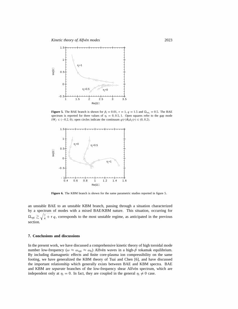
Figures 5 and 6 show the same parametric studies and use the same conventions offigures 1 and 2, except that here∗ni = 0.5. The same considerations which were madein the previous case hold here. In contrast, figures 7 and 8, where∗ni = 3, exhibit newqualitative features of the BAE/KBM spectra. First of all, the BAE branch never becomes

Kinetic theory of Alfv´en modes 2021

1.5 2 2.5 3 3.5- 1

- 0 . 5

0

0.5

1

1.5

Re(Ω)

Im(Ω

)

ηi=0.5

ηi=0.25

ηi=0

Figure 1. The BAE branch is shown forβi = 0.01, τ = 1, q = 1.5 and∗ni = 1. The BAEspectrum is reported for three values ofηi = 0, 0.25, 0.5. Open squares refer to the gap modeδWf ∈ (−0.2, 0); open circles indicate the continuumq(r)R0k‖(r) ∈ (0, 0.2).

0.9 1 1.1 1.2 1.3 1.4 1.5 1.6 1.7- 1

- 0 . 5

0

0.5

1

1.5

Re(Ω)

Im(Ω

)

ηi=0 η

i=0.25

ηi=0.5

Figure 2. The KBM branch is shown for the same parametric studies reported in figure 1.

unstable; second, even if a value forηi can still be identified (between 0.5 and 1), abovewhich BAE and KBM strongly couple, this value can no longer be considered as a thresholdfor the continuous spectrum to be unstable. In fact, Im at the most unstable (that of KBM)accumulation point is exponentially small, as predicted by equation (27). The difference with

respect to the previous cases is entirely due to the value of∗ni . For ∗pi <

√74 + τ q, the

features of the BAE/KBM spectrum are those of figures 1, 2 and 5, 6. The dominant modesfor ηi > ηic are those of the BAE branch, and in this case part of the continuous Alfven

spectrum is unstable. In the∗pi >

√74 + τ q case, however, the features of the BAE/KBM

spectrum are those of figures 7 and 8. The dominant modes are of the KBM branch andthe Alfven continuum is always stable (it coincides with that predicted in ideal MHD withdiamagnetic effects included). The present discussion is consistent with the statement, madein the previous section, that the KBM accumulation point has an exponentially small Im

for ∗pi >

√74 + τ q.

2022 F Zonca et al

-0 .02

-0.015

-0 .01

-0.005

0

- 3 . 7 - 3 . 6 - 3 . 5 - 3 . 4 - 3 . 3 - 3 . 2 - 3 . 1 - 3

Im(Ω

)

Re(Ω)

ηi=0

ηi=0.5

ηi=0.25

Figure 3. The branch propagating in the electron diamagnetic drift direction is shown for thesame parametric studies reported in figure 1.

1.4 1.6 1.8 2 2.2 2.4- 1

- 0 . 5

0

0.5

1

Re(Ω)

Im(Ω

)

ηi=0.25

ηi=0.28

ηi=0.25

ηi=0.28

Figure 4. Two spectra withηi = 0.25 andηi = 0.28 illustrate the coupling of BAE (opencircles) and KBM (open squares) branches.δWf ∈ (−0.14, −0.06) in all cases. Equilibriumparameters are those of figure 1.

For ∗pi ≈√

74 + τ q, BAE and KBM branches are strongly coupled. In the previous

section, it was anticipated that in this parameter range Im of the unstable BAE/KBMaccumulation point is expected to be peaked. This aspect is examined in figures 9 and10, where imaginary and real parts of the BAE/KBM accumulation point are respectivelyshown against∗ni and for different values ofηi . Open circles refer to theηi = 0.5

case, open squares toηi = 1.0 and open triangles toηi = 1.5. For ∗pi √

74 + τ q, the

numerical results are well described by the analytical estimate, equation (30), indicating thatthe unstable accumulation point is of BAE type (note thatηi > ηic). In fact, Im increases

linearly with both∗ni andηi , whereas Re linearly decreases. When∗pi ≈√

74 + τ q,

the strong coupling of BAE with KBM results in the break down of equation (30): Re

begins to increase and the behaviour of Im is no longer linear. Finally, the dependence of

the unstable accumulation point on∗ni andηi becomes of KBM type for∗pi √

74 + τ q,

as predicted by equation (27). Thus, figures 9 and 10 illustrate the smooth transition from

Kinetic theory of Alfv´en modes 2023

- 0 . 5

0

0.5

1

1.5

1 1.5 2 2.5 3 3.5

Im(Ω

)

Re(Ω)

ηi=1

ηi=0.5 η

i=0

Figure 5. The BAE branch is shown forβi = 0.01, τ = 1, q = 1.5 and∗ni = 0.5. The BAEspectrum is reported for three values ofηi = 0, 0.5, 1. Open squares refer to the gap modeδWf ∈ (−0.2, 0); open circles indicate the continuumq(r)R0k‖(r) ∈ (0, 0.2).

- 1

- 0 . 5

0

0.5

1

1.5

0.4 0.6 0.8 1 1.2 1.4 1.6

Im(Ω

)

Re(Ω)

ηi=0 η

i=0.5

ηi=1

Figure 6. The KBM branch is shown for the same parametric studies reported in figure 5.

an unstable BAE to an unstable KBM branch, passing through a situation characterizedby a spectrum of modes with a mixed BAE/KBM nature. This situation, occurring for

∗pi &√

74 + τ q, corresponds to the most unstable regime, as anticipated in the previous

section.

7. Conclusions and discussions

In the present work, we have discussed a comprehensive kinetic theory of high toroidal modenumber low-frequency (ω ≈ ω∗pi ≈ ωti ) Alfv en waves in a high-β tokamak equilibrium.By including diamagnetic effects and finite core-plasma ion compressibility on the samefooting, we have generalized the KBM theory of Tsai and Chen [6], and have discussedthe important relationship which generally exists between BAE and KBM spectra. BAEand KBM areseparatebranches of the low-frequency shear Alfven spectrum, which areindependent only atηi = 0. In fact, they are coupled in the generalηi 6= 0 case.

2024 F Zonca et al

- 1 . 2

- 1

- 0 . 8

- 0 . 6

- 0 . 4

- 0 . 2

0

1.5 2 2.5 3 3.5 4 4.5

Im(Ω

)

Re(Ω)

ηi=0 η

i=0.5 η

i=1

Figure 7. The BAE branch is shown forβi = 0.01, τ = 1, q = 1.5 and∗ni = 3. The BAEspectrum is reported for three values ofηi = 0, 0.5, 1. Open squares refer to the gap modeδWf ∈ (−0.2, 0); open circles indicate the continuumq(r)R0k‖(r) ∈ (0, 0.2).

- 0 . 5

0

0.5

1

1.5

2 3 4 5 6 7

Im(Ω

)

Re(Ω)

ηi=0 η

i=0.5

ηi=1

Figure 8. The KBM branch is shown for the same parametric studies reported in figure 7.

It has been shown that the theory of [6] applies forω∗pi √

74 + τqωti , as expected, a

condition under which KBM are the most unstable modes of those considered here. Moreimportantly, we have demonstrated that, forω∗pi <

√74 + τqωti , a critical valueηic exists,

above which the BAE mode is the most unstable branch, thereby showing that BAEs arenot always Landau damped as simple considerations based on its frequency would suggest[16]. It has also been shown that, forηi > ηic, part of the continuous Alfven spectrum maybe unstable. This implies that non-collective modes may be present in the plasma, formedas a superposition of local oscillations which are quasi-exponentially growing in time. Thisnew feature is entirely due to the inclusion of finite core-plasma ion compressibility in thetheoretical analysis. Finally, it has been shown that the most unstable low-frequency Alfven

modes occur atω∗pi &√

74 + τqωti , corresponding to a parameter range in which BAE and

KBM are strongly coupled.The present theory of BAE/KBM linear stability yields an analytic expression of the

mode dispersion relation, which may be generalized to include resonant wave excitations

Kinetic theory of Alfv´en modes 2025

- 0 . 2

0

0.2

0.4

0.6

0.8

1

1.2

0 0.5 1 1.5 2 2.5 3 3.5 4

Im(Ω

)

Ω*ni

ηi=0.5

ηi=1.5

ηi=1.0

Figure 9. Im() of the most unstable BAE/KBM accumulation point is shown against∗ni

for βi = 0.01, τ = 1, q = 1.5, δWf = 0 and different values ofηi : ηi = 0.5 (open circles),ηi = 1.0 (open squares) andηi = 1.5 (open triangles).

2

2.5

3

3.5

4

4.5

0 0.5 1 1.5 2 2.5 3 3.5 4

Re(

Ω)

Ω*ni

ηi=1.5

ηi=1.0

ηi=0.5

Figure 10. Re() of the most unstable BAE/KBM accumulation point is shown against∗ni

for the same parameters of figure 9.

by energetic particles with finite orbit widths [6]. It has been shown that, in general, twotypes of spectra may exist: a discrete spectrum of gap modes, which is present only whenthe tokamak plasma is ideal MHD unstable; and the Alfven continuous spectrum, whichmay be characterized, under certain conditions, by unstable accumulation points.

The issue of energetic particle continuum modes [6], which may also exist forδWf > 0,but require that the energetic particle drive be strong enough to overcome continuumdamping, is not analysed here. The numerical studies of the analytic dispersion relation dealonly with BAE/KBM gap modes and with the Alfven continuous spectrum. Finally, it isclear that the present theoretical results may have important implications for the stability andtransport properties of tokamak experiments with and without energetic particles. Furthertheoretical delineations and comparisons with experimental results are, however, beyond thescope intended for this work and will be discussed in future publications.

2026 F Zonca et al

Acknowledgments

This work was supported by the US Department of Energy, DOE DE-FG03-94ER54271, theNational Science Foundation, NSF grant ATM-9396158, and the University of CaliforniaEnergy Institute, UCEI-20594. One author, FZ, is grateful to the Department of Physicsand Astronomy, University of California at Irvine for the hospitality and support receivedduring the period in which part of this work was done.

Appendix A. Validity of the ideal MHD limit δE‖ = 0

At order O(β), the quasi-neutrality equation, equation (5), becomes(1

τ+ ω∗ni

ω

)(δ8(0) − δ9(0)) +

(1 − ω∗pi

ω

)biδ9

(0) = Tik⊥nekϑ

⟨−k2

⊥ρ2Li

4δK

(0)

i + δK(2)

i

⟩.

(A1)

Here,δK(2)

i is obtained from

(ωtr∂θ0 − iω)δK(2)

i = −(ωtr∂θ1 + iωdi)δK(1)

i + i

(ekϑ

mik⊥

)×QF0i

[(δ8(2) − δ9(2)) − k2

⊥ρ2Li

4(δ8(0) − δ9(0)) + miv

2⊥

2eBδB

(0)‖

]. (A2)

In order to get from equation (A1) an expression for(δ8(0) − δ9(0)) valid up to O(β), we

need to solve equation (A2) just forδK(2)

i , where[...] = (1/2π)∮(...) dθ0. It is possible to

show that

δK(2)

i =(

ekϑ

mik⊥

)QF0i

ω

[k2⊥ρ2

Li

4(δ8(0) − δ9(0)) − miv

2⊥

2eBδB

(0)‖

]− i

ωtr

ω∂θ1δK

(1)

i + ωdi

ωδK

(1)

i .

(A3)

When substituted into equation (A1), equation (A3) yields the O(β) quasi-neutralitycondition, reported in section 3:

ω2ti

2ω2

(1 − ω∗pi

ω

) k⊥kϑ

∂2

∂θ21

[kϑ

k⊥(δ8(0) − δ9(0))

]+

(1

τ+ ω∗ni

ω

)(δ8(0) − δ9(0))

+(

1 − ω∗pi

ω

)bi + q2bi

ωti

ω

[(1 − ω∗ni

ω

)F(ω/ωti)

−ω∗Ti

ωG(ω/ωti) − N2(ω/ωti)

D(ω/ωti)

]δ8(0)

= b1/2i α

23/2q

ωti

ω

kϑ

k⊥

(1 − ω∗pi

ω

)δ9(0). (A4)

Equation (A4) demonstrates that(δ8(0) −δ9(0)) = O(β), i.e. δE‖ ' 0, for long wavelengthmodes (∂θ1 = O(β1/2)) with ω∗pi/ω = O(1) and which propagate in the ion diamagneticdirection ((1/τ + ω∗ni /ω) = O(1)). In the present paper, we refer to this type of mode.

For waves which propagate in the electron diamagnetic direction, equation (A4) predictsthat an appreciable parallel electric field can be originated for(1/τ + ω∗ni /ω) = O(bi).Another possibility for theδE‖ ' 0 assumption to break down isω∗pi/ω = O(1/β). Thesemodes would interact strongly with the long wavelength slab-like ion temperature gradient(ITG) driven mode [7–9] and are out of the scope of the present analysis.

Kinetic theory of Alfv´en modes 2027

Equation (A4) serves also to the scope of discussing the validity of theδE‖ = 0assumption at moderate|θ | values. In fact, for|θ | < O(β−1/2) finite bi andωdi/ω effectsmay be neglected, indicating that the scale of variation of(δ8(0) − δ9(0)) is a constant.This can be also seen from a direct examination of equations (2) and (5). Moreover, sincethe large|θ | structure of the modes we are analysing is characterized by a long scale ofvariation, we must also have∂θ = constant = O(β1/2) when acting on(δ8(0) − δ9(0))

for |θ | < O(β−1/2). Recalling that(1/τ + ω∗ni /ω) and ω∗pi/ω are O(1) in our analysis,the present argument and equation (A4) indicate thatδE‖ = 0 to lowest order also formoderate|θ | values, i.e.(δ8(0) − δ9(0)) = 0. The fact that∂θ = O(β1/2) when acting on(δ8(0) − δ9(0)) does not indicate that the functionsδ8(0) andδ9(0) vary on the long scaleθ1 only, but simply that any short-scale variation ofδ8(0) is balanced by the same variationof δ9(0).

The previous discussion demonstrates that the(δ8(0)−δ9(0)) = 0 assumption also holdsin the moderate|θ | region, whereδ9(0) does not have a two-scale structure, as pointed outin section 3.2, and, in general,∂θ = O(1) due to finite(s, α) effects, as it emerges fromequation (15).

Appendix B. Logarithmic singularities and continuous spectrum

A simple derivation of equation (23) can be obtained transforming the ballooningeigenfunctionδψ(θ) = [kϑ/k⊥(θ)]δ9(θ) back to real space [17]

δψ(nq − m) =∫ +∞

−∞

δ9(θ) exp[−i(nq − m)θ ]

[1 + (sθ − α sinθ)2]1/2dθ. (B1)

From equation (B1), it is easily shown that

is∂δψ(nq − m)

∂(nq − m)=

∫ +∞

−∞

sθδ9(θ) exp[−i(nq − m)θ ]

[1 + (sθ − α sinθ)2]1/2dθ. (B2)

Define, now, a value2 such that2 1 andβ1/22 1. In this way, the integration intervalin equation (B2) can be subdivided into [−2, 2], where the ‘ideal’ solutionδ9ID can beused, and(−∞, −2] ∪ [2, +∞), where the ‘inertial layer’ solutionδ9IN is appropriate.With the explicit use of equation (18), it is possible to show

is∂ δψ(nq − m)

∂(nq − m)=

∫ 2

−2

sθδ9ID(θ) exp[−i(nq − m)θ ]

[1 + (sθ − α sinθ)2]1/2dθ

+∫ ∞

2

[exp i(m − nq)θ − exp i(nq − m)θ ] ei3θ dθ

+O

(1

s222

)+ O

( α

s2

)+ O

(1

2

). (B3)

Since the contribution from the [−2, 2] integral is typically O(2), whereas that from the[2, ∞) interval is O(β−1/2) for |nq − m| = O(β1/2), equation (B3) implies

s∂ δψ(nq − m)

∂(nq − m)=

[exp i2(m − nq)

3 − (nq − m)− exp i2(nq − m)

3 + (nq − m)

]ei32 + O

(1

s222

)+O

( α

s2

)+ O

(1

2

)+ O(β1/22). (B4)

Equation (B4) is readily integrated and yields

δψ(nq − m) = C − 1

sln[32 − (nq − m)2] (B5)

2028 F Zonca et al

for |nq −m| ≈ |3| = O(β1/2), where C is an integration constant and O(β1/22) terms havebeen consistently neglected. Equation (B5) indicates that the wave field in real space has alogarithmic singularity when(nq − m) = ±3, i.e. when

q(r)R0k‖(r) = ±3(ω(r))

which is equation (23). In an initial-value analysis, the just derived logarithmic singularitybecomes a logarithmic branch point in the complex omega plane. When the time asymptoticbehaviour is computed, the finite jump of the wave field across the branch cut, originatingfrom the logarithmic branch point, gives the contribution

1

texp(−iω(r)t)

of equation (22). A detailed analysis, yielding to this result, can be found in [14]. Here,we just wish to note that the concepts of continuous spectrum, satisfying equation (23), andof singular local plasma oscillations are closely related.

References

[1] Heidbrink W W, Strait E J, Chu M S and Turnbull A D 1993 Phys. Rev. Lett.71 855[2] Cheng C Z, Chen L, Chance M S 1985Ann. Phys.161 21[3] Turnbull A D, Strait E J, Heidbrink W W, Chu M S, Greene J M, Lao L L, Taylor T S and Thompson S J

1993Phys. FluidsB 5 2546[4] Chu M S, Greene J M, Lao L L, Turnbull A D and Chance M S 1992Phys. FluidsB 4 3713[5] Biglari H and Chen L 1991Phys. Rev. Lett.67 3681[6] Tsai S T and Chen L 1993Phys. FluidsB 5 3284[7] Chen L, Briguglio S and Romanelli F 1991Phys. FluidsB 3 611[8] Romanelli F, Chen L and Briguglio S 1991Phys. FluidsB 3 2496[9] Guo S C and Romanelli F 1994Phys. Plasmas1 1101

[10] Connor J W, Hastie R J and Taylor J B 1978Phys. Rev. Lett.40 396[11] Antonsen T M and Lane B 1980Phys. Fluids23 1205[12] Chen L and Hasegawa A 1991J. Geophys. Res.96 1503[13] Romanelli F and Chen L 1991Phys. FluidsB 3 329[14] Sedlacek Z 1971J. Plas. Phys.5 239[15] Santoro R A and Chen L 1996Phys. Plasmas3 2349[16] Betti R, Berk H L and Freidberg J P 1994Bull. Am. Phys. Soc.39 1702[17] Zonca F and Chen L 1993Phys. FluidsB 5 3668