arX

iv:1

007.

2892

v2 [

mat

h-ph

] 1

5 N

ov 2

010

Kinematics of finite elastic and plastic deformations

Tamas Fulop1,3 and Peter Van1,2,3

1 KFKI Research Institute for Particle and Nuclear Physics,

Konkoly-Thege M. ut 29-33, H-1121, Budapest, Hungary

2 Dept. of Energy Engineering, Budapest Univ. of Technology and Economics,

Bertalan Lajos u. 4-6, H-1111, Budapest, Hungary

3 Montavid Thermodynamic Research Group,

Igmandi u. 26. fsz. 4, H-1112, Budapest, Hungary

November 16, 2010

Abstract

The kinematics of finite elastic and plastic deformations is considered in an approach

that does not rely on reference frame and reference configuration, and that gives account

of the inertial-noninertial aspects explicitly. These features are achieved by working

on nonrelativistic spacetime directly. The quantity measuring elastic deformations is

introduced according to its physical role, and the definition of the quantity describing

plastic changes follows as a natural consequence. The properties of both are analyzed,

and their relationship to frequently used elastic and plastic kinematic quantities is

discussed. One important result is that neither the elastic nor the plastic kinematic

quantity can be defined from deformation gradient.

1 Introduction

Kinematics of continua is an old area, with a lot of contributions from very many scien-tists. Still, it is not a closed subject. A number of open questions, controversial aspects andproblems stimulate further research. These problematic issues become particularly relevantwhen moving from small elastic and plastic deformations to large, from slow processes tofast, from essentially homogeneous bodies to considerably inhomogeneous settings — as isthe case with nanostructures —, and from simple continua to ones with such microstructurethat plays important role also at the macro level and where the kinematics of the microprocesses is to be established and to be brought into harmony with the macro kinematics.Therefore, the open questions should be answered and kinematics must be made ready forthe new and newer demands.

The approach to finite (i.e., not necessarily small) elastic and plastic deformations pre-sented here intends to stay on the safe side — safe from the controversial problems. Themethodology used is chosen according to this purpose. It has the following basic pillars.

1. The mathematical model is seriously distinguished from physical reality.

2. Nonetheless, it is constructed to express the relevant physical requirements, not lessand not more.

3. Embodying this, avoided are any auxiliary elements, which could make the descriptiontechnically more convenient but do not belong to the physics of the motion of thecontinuum.

4. As an example, nonrelativistic spacetime is considered in the reference frame free —affine space based — formulation.

5. Similarly, the continuum is considered as a smooth manifold, but it is equipped aswell by some further structures as dictated by physical requirements. Meanwhile, no

1

convenience-motivated auxiliary elements are introduced for the elastic and plastickinematics of the material.

The treatment of objectivity is one of the important aspects of this paper. In nonrela-tivistic physics, the spacetime is seemingly rather simple and transparent, therefore the needfor the very concept of spacetime is not apparent. Usually, the notion of spacetime is left im-plicit and objectivity is formulated in an indirect way, with the help of invariance propertiesunder changes of special (rigid) reference frames. This kind of approach can be combinedwith differential geometry for the spacelike part of the corresponding physical quantities, too(see e.g. [1, 2, 3]). However, restricting ourselves to the transformation of reference framesrelated to spacelike part of physical quantities neglecting their time dependence results in animproper (or at least insufficient) formulation of covariance as one can demonstrate by theusual rigid observers of Noll [4]. Therefore, the need for a reference frame free formulationof continuum physics is indicated by several authors [5, 6] and some realizations, slightlysimilar to our approach, already exist in the literature1. In our treatment, spacetime has anexplicit mathematical structure, which clearly shows the unavoidable nontrivial intertwiningof space and time, even nonrelativistically. The reference frame independence of the basicphysical quantities is ensured by formulation - physical quantities are given as spacetimecompatible objects. The need for such a kind of approach to nonrelativistic spacetime hasbeen indicated some time ago [11, 12], and a fully elaborated formulation was given first in[13].

In this paper, we investigate kinematics of elastic and plastic continua, the literatureof which is still far too extensive to give a fair account of it. To list at least a part ofthe works that are closely related to the ideas raised here, [14] is one of the definitivecontributions, [15] connects the finite deformation compatibility condition with the vanishingof a Riemann curvature, Bertram [16] provides a good collection of the problematic issuesof kinematics, DiCarlo [17] quotes and uses the notions of current configuration and relaxedconfiguration, and Epstein [18] and Leon [19] are two examples for sources that operate withthe term reference crystal. For the methodology of mathematical models in physics, [13] isan advanced, and [20] is a more readable source. The latter is also the most comprehensivesource for the frame free formulation of spacetime. As such, it can also be consulted for themathematical treatment of the various quantities with physical dimensions: lengths, times,masses etc., for tensorial operations (identifications, dual transpose, metric adjoint), and foraffine spaces.

The paper is organized as follows. First, the standard formulation of kinematics is sur-veyed. Then, some questionable aspects of the customary notions of finite deformationkinematics are highlighted. This is followed by a summary of the frame free formalism ofnonrelativistic spacetime, a necessary ingredient for the forthcoming considerations. Thefifth section defines the kinematics of a solid in spacetime. The subsequent section derivesthe kinematic quantities needed for elasticity, the elastic shape - a frame independent gener-alized deformation -, and the elastic deformedness - a frame independent generalized strain.The resulting compatibility condition is calculated, too. The last section lays the foundationof plastic kinematics. Finally, a concise summary is given.

2 A standard formulation of kinematics

So as to set the context for expressing the motivations, let us start with summarizing ausual approach to elastic and plastic kinematics.

This starts with choosing a reference frame—this step being taken only tacitly, usually.Next, the continuum is represented by a reference configuration, i.e., by its location in thespace of this frame at a chosen reference instant t0 . More closely, each material point isrepresented by its position X in this space at t0 . At time t , the position of a materialpoint is x = χt(X), and its velocity is vt(X) = χt(X), where overdot means partial

1See the publications of Walter Noll about the foundations of continuum mechanics starting from [7]and more recently on his website (http://www.math.cmu.edu/ wn0g/noll/). Here, he emphasizes e.g. theneed of affine spaces ([8], p24, but later on he introduces some slightly different concepts [9]). However,nonrelativistic spacetime remains implicit and time is separated in his kinematics [10].

2

derivative with respect to time, ˙ = ∂t∣∣X. With the displacement since t0 ,

ut(X) := χt(X)−X , (1)

one also has

v = u . (2)

The so-called deformation gradient is introduced as

F := χ⊗∇X , (3)

with ⊗ denoting dyadic/tensorial product; in what follows, the partial derivative operation∇

Xwill act to the left or to the right depending on context, always to reflect the proper

tensorial order (‘order of tensorial indices’). The deformation gradient is assumed to beinvertible. This is ensured if one requires that detF (which is the Jacobian of the map χ )is nonzero, which physically means that the continuum can never be singularly compressed.Following from its definition, F obeys the properties

F = v⊗∇X, FF−1 = v⊗∇x, (F⊗∇X)A2,3 = 0 ; (4)

where in the middle formula velocity is considered in variables t,x [the connection with thevariables t,X being established by χt(X) ], and in the last formula antisymmetrization iscarried out in the second and third ‘indices’. Similarly, S will stand for symmetric part, T

for transpose and tr for trace, and, for example, tr1,3 will denote contraction of the firstand third ‘indices’. Note that, according to the chain rule of differentiation of compositefunctions, a multiplication by F from the right gives the transition from the derivative ∇x

of a quantity to the derivative ∇X

(and multiplication by F−1 from the right gives theopposite direction).

Related to this, if one has a process from t0 to t2 then, for any t1 in between,

F(t0)t2

= F(t1)t2

F(t0)t1

(5)

where t1 is also used as another reference instant, and that’s why now the used referenceinstants are also displayed in superscript. As a special case,

F(t0)t1

=[F

(t1)t0

]−1

. (6)

The deformation gradient — as assumed to be invertible — admits a polar decomposi-tion:

F = ULO = OUR , (7)

with orthogonal O and symmetric and positive definite UL =√FFT, UR =

√FTF .

The various deformation tensors (Cauchy-Green, Finger, . . . ) are defined as variouspowers of UL and UR :

C(n)L := (UL)

n, C

(n)R := (UR)

n. (n = . . . ,−2,−1, 0, 1, 2, . . .). (8)

From them, the various strain tensors (Green-Lagrange, St. Venant, Biot, Almansi, Hencky,. . . ) are derived, all expressing in some way the deviation from the identity tensor I :

E(n)L :=

1

n

[C

(n)L − I

]=

1

n

[(UL)

n − I], E

(0)L := lnUL, (9)

E(n)R :=

1

n

[C

(n)R − I

]=

1

n

[(UR)

n − I], E

(0)R := lnUR (10)

[the n = 0 cases (Hencky strains) being the l’Hopital limits of the n 6= 0 series]. In addition,the Cauchy strain — with which each of the above strains coincides in the leading order ofF− I , i.e., for small strains — is defined as

ECauchy = FS − I = (χ⊗∇X)S − I = (u⊗∇X)

S. (11)

3

The important dynamical purpose with strain is to use it as the variable on which elasticinner forces — described by the elastic stress tensor — and the corresponding elastic energyare assumed to depend.

When plastic changes also occur in a material, kinematics needs to describe what a plasticchange is geometrically, and how it differs from elastic changes. One usual approach is toassume that strain (one of the definitions above, typically ECauchy ) decomposes into a sum,

Etotal = Eelast +Eplast , (12)

and another conception, considered more applicable for nonsmall deformations, decomposesthe deformation gradient, instead, and does it multiplicatively:

Ftotal = FelastFplast . (13)

The latter may be explained that, after a subsequent complete elastic relaxation, whichwould bring in multiplication by (Felast)−1 from the left [in accord with (5) and (6)], onewould obtain what the plastic deformation is, and one would reach the relaxed configuration.

3 Remarks and observations

The following remarks and observations will help in giving motivations and hints for animprovement of kinematics.

3.1 So many strains

Probably the most immediate observation is that there are many, actually infinitely manydefinitions for deformation and for strain. In addition, it is not hard to introduce infinitelymany further — and not unreasonable — versions. Then, which one to use as the variableof an elastic constitutive relation? In linear elasticity, in which strain the elastic constitutiverelation is expected to be the most linear? For instance, Horgan and Murphy [21] finds

that, for large deformations of hard rubber, among the E(n)R strains, n = 0 provides the

most precise linearity and in the largest regime. In parallel, in nonlinear elasticity, fittingexperimental data to a nonlinear elastic constitutive relation, e.g., to the Murnaghan model,can provide unphysical values for the material coefficients, and with large uncertainties,when, for example, the n = 2 strain is used. When n = 0 is chosen, instead, then theresults are much more realistic and much more reliable [22].

To summarize, there is no satisfactory amount of knowledge collected and distributedabout the relevance of the various strain measures.

3.2 Volumetric properties towards infinities and in between

A less apparent, but not unimportant, aspect is that the strains (9)–(10) with positive n takefinite value in the infinitely compressed singular limit ( detF → 0 ). On the other side, thecases with negative n take finite value in the infinitely expanded asymptotics ( detF → ∞ ).A geometrically really descriptive strain quantity would diverge in both these singular limits.Also, it is such a quantity from which good numerical stability could be expected. Namely,if, by numerical error, the numerical representation of the system starts to deviate towardslarge extension or compression, such a strain measures it sensitively, and the proportionaladditional elastic forces will drive the situation back towards the correct value.

In this respect, the Hencky strains do better than the others listed above, as they divergein both asymptotics. This, therefore, provides as well a possible explanation of the findingsof [22] mentioned previously.

At this point, it is worth asking the following question, too. For small deformations,the Cauchy strain is known to describe the purely volumetric changes by its spherical part(trace part), and purely torsional ones by its deviatoric part. Is there such a strain — oneamong those mentioned above, or some other one — that admits the same property for finitedeformations as well?

Actually, one finds that the left and right Hencky strains (n = 0 ) satisfy this criterionas well. This can be shown as follows.

4

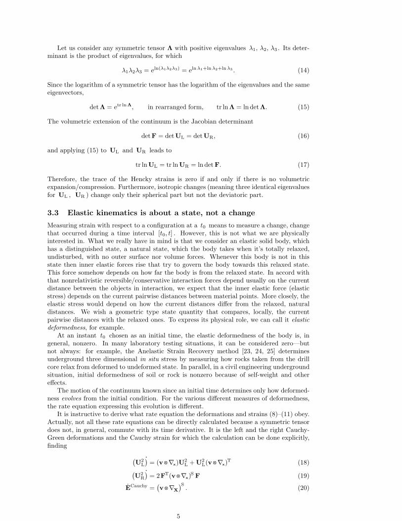
Let us consider any symmetric tensor Λ with positive eigenvalues λ1, λ2, λ3 . Its deter-minant is the product of eigenvalues, for which

λ1λ2λ3 = eln(λ1λ2λ3) = e

lnλ1+lnλ2+lnλ3 . (14)

Since the logarithm of a symmetric tensor has the logarithm of the eigenvalues and the sameeigenvectors,

detΛ = etr lnΛ, in rearranged form, tr lnΛ = ln detΛ. (15)

The volumetric extension of the continuum is the Jacobian determinant

detF = detUL = detUR, (16)

and applying (15) to UL and UR leads to

tr lnUL = tr lnUR = ln detF. (17)

Therefore, the trace of the Hencky strains is zero if and only if there is no volumetricexpansion/compression. Furthermore, isotropic changes (meaning three identical eigenvaluesfor UL , UR ) change only their spherical part but not the deviatoric part.

3.3 Elastic kinematics is about a state, not a change

Measuring strain with respect to a configuration at a t0 means to measure a change, changethat occurred during a time interval [t0, t] . However, this is not what we are physicallyinterested in. What we really have in mind is that we consider an elastic solid body, whichhas a distinguished state, a natural state, which the body takes when it’s totally relaxed,undisturbed, with no outer surface nor volume forces. Whenever this body is not in thisstate then inner elastic forces rise that try to govern the body towards this relaxed state.This force somehow depends on how far the body is from the relaxed state. In accord withthat nonrelativistic reversible/conservative interaction forces depend usually on the currentdistance between the objects in interaction, we expect that the inner elastic force (elasticstress) depends on the current pairwise distances between material points. More closely, theelastic stress would depend on how the current distances differ from the relaxed, naturaldistances. We wish a geometric type state quantity that compares, locally, the currentpairwise distances with the relaxed ones. To express its physical role, we can call it elasticdeformedness, for example.

At an instant t0 chosen as an initial time, the elastic deformedness of the body is, ingeneral, nonzero. In many laboratory testing situations, it can be considered zero—butnot always: for example, the Anelastic Strain Recovery method [23, 24, 25] determinesunderground three dimensional in situ stress by measuring how rocks taken from the drillcore relax from deformed to undeformed state. In parallel, in a civil engineering undergroundsituation, initial deformedness of soil or rock is nonzero because of self-weight and othereffects.

The motion of the continuum known since an initial time determines only how deformed-ness evolves from the initial condition. For the various different measures of deformedness,the rate equation expressing this evolution is different.

It is instructive to derive what rate equation the deformations and strains (8)–(11) obey.Actually, not all these rate equations can be directly calculated because a symmetric tensordoes not, in general, commute with its time derivative. It is the left and the right Cauchy-Green deformations and the Cauchy strain for which the calculation can be done explicitly,finding

(U2

L

.)= (v⊗∇x)U

2L +U2

L(v⊗∇x)T (18)

(U2

R

.)= 2FT(v⊗∇x)

S F (19)

ECauchy =(v⊗∇

X

)S. (20)

5

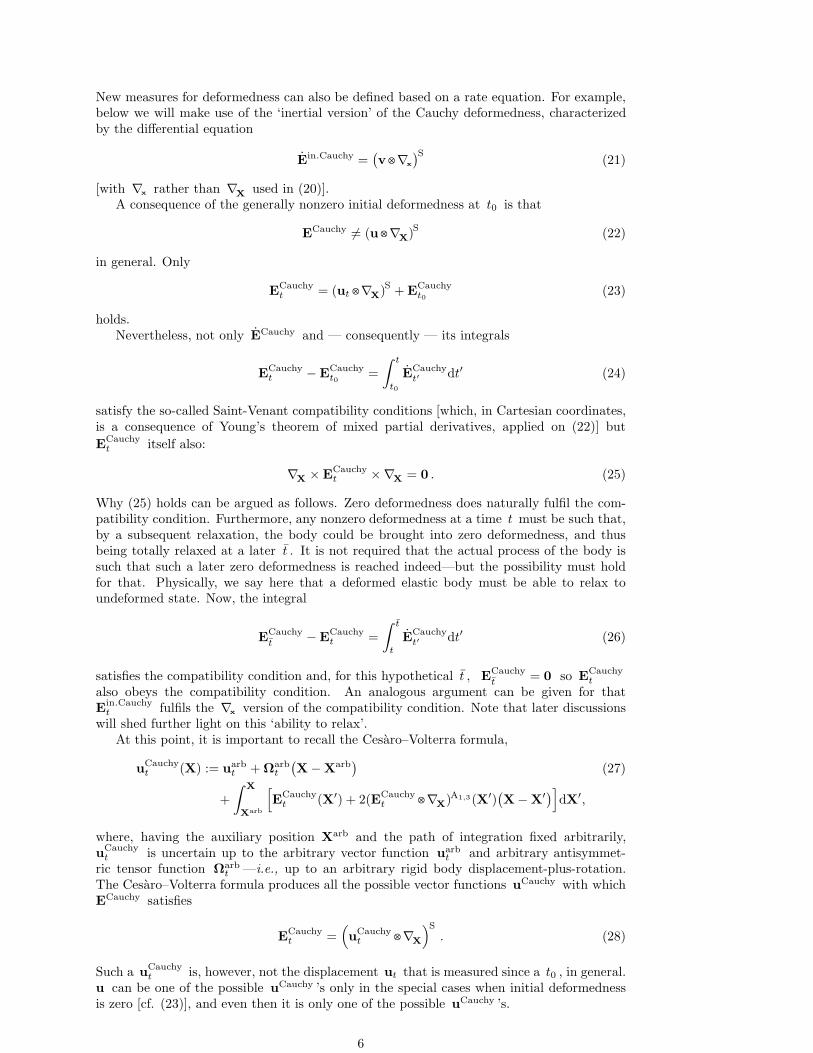
New measures for deformedness can also be defined based on a rate equation. For example,below we will make use of the ‘inertial version’ of the Cauchy deformedness, characterizedby the differential equation

Ein.Cauchy =(v⊗∇x

)S(21)

[with ∇x rather than ∇X

used in (20)].A consequence of the generally nonzero initial deformedness at t0 is that

ECauchy 6= (u⊗∇X)S (22)

in general. Only

ECauchyt = (ut ⊗∇

X)S +E

Cauchyt0

(23)

holds.Nevertheless, not only ECauchy and — consequently — its integrals

ECauchyt −E

Cauchyt0

=

∫ t

t0

ECauchyt′ dt′ (24)

satisfy the so-called Saint-Venant compatibility conditions [which, in Cartesian coordinates,is a consequence of Young’s theorem of mixed partial derivatives, applied on (22)] but

ECauchyt itself also:

∇X ×ECauchyt ×∇X = 0 . (25)

Why (25) holds can be argued as follows. Zero deformedness does naturally fulfil the com-patibility condition. Furthermore, any nonzero deformedness at a time t must be such that,by a subsequent relaxation, the body could be brought into zero deformedness, and thusbeing totally relaxed at a later t . It is not required that the actual process of the body issuch that such a later zero deformedness is reached indeed—but the possibility must holdfor that. Physically, we say here that a deformed elastic body must be able to relax toundeformed state. Now, the integral

ECauchyt

−ECauchyt =

∫ t

t

ECauchyt′ dt′ (26)

satisfies the compatibility condition and, for this hypothetical t , ECauchyt

= 0 so ECauchyt

also obeys the compatibility condition. An analogous argument can be given for thatE

in.Cauchyt fulfils the ∇x version of the compatibility condition. Note that later discussions

will shed further light on this ‘ability to relax’.At this point, it is important to recall the Cesaro–Volterra formula,

uCauchyt (X) := uarb

t +Ωarbt

(X−Xarb

)(27)

+

∫X

Xarb

[E

Cauchyt (X′) + 2(ECauchy

t⊗∇

X)A1,3(X′)

(X−X′

)]dX′,

where, having the auxiliary position Xarb and the path of integration fixed arbitrarily,uCauchyt is uncertain up to the arbitrary vector function uarb

t and arbitrary antisymmet-ric tensor function Ωarb

t —i.e., up to an arbitrary rigid body displacement-plus-rotation.The Cesaro–Volterra formula produces all the possible vector functions uCauchy with whichECauchy satisfies

ECauchyt =

(uCauchyt

⊗∇X

)S. (28)

Such a uCauchyt is, however, not the displacement ut that is measured since a t0 , in general.

u can be one of the possible uCauchy ’s only in the special cases when initial deformednessis zero [cf. (23)], and even then it is only one of the possible uCauchy ’s.

6

A uCauchy is to be considered as a vectorial type potential for a symmetric tensor thatsatisfies Saint-Venant’s compatibility condition, the condition to admit zero left-plus-rightcurl. Indeed, this situation is an analogue of that a curl free vector field admits a scalar po-tential, which is non-unique and can be obtained from the vector field via its integral alongan arbitrary curve. By this analogy, uCauchy can be named a Cauchy potential of a Cauchytype tensor field (a symmetric tensor field with the Saint-Venant property). This namingexplains the superscript Cauchy in the notation uCauchy . A Cauchy potential is a mathemat-ical auxiliary quantity, which is in general unrelated to the physical displacement quantity:the indeterminateness in uCauchy allows displacement only as a special case of uCauchy , andeven the possibility for this special choice is ruined by nonzero initial deformedness. Cauchypotential and displacement are only occasionally and weakly related quantities. These twonotions should never be confused.

For later use, let us give here a rewritten form of (28),

ECauchyt =

[(X+ u

Cauchyt

)⊗∇X − I

]S, (29)

too, despite that, at the moment, not any usefulness of this version is apparent.

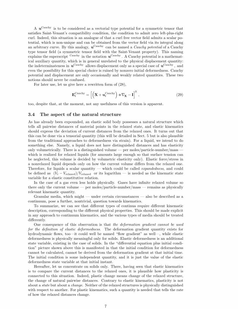
3.4 The aspect of the natural structure

As has already been expounded, an elastic solid body possesses a natural structure whichtells all pairwise distances of material points in the relaxed state, and elastic kinematicsshould express the deviation of current distances from the relaxed ones. It turns out thatthis can be done via a tensorial quantity (this will be detailed in Sect. 5 but is also plausiblefrom the traditional approaches to deformedness via strain). For a liquid, we intend to dosomething else. Namely, a liquid does not have distinguished distances and has elasticityonly volumetrically. There is a distinguished volume — per moles/particle-number/mass —which is realized for relaxed liquids (for amounts large enough so that surface tension canbe neglected, this volume is decided by volumetric elasticity only). Elastic force/stress ina nonrelaxed liquid depends only on how the current volume differs from the relaxed one.Therefore, for liquids a scalar quantity — which could be called expandedness, and couldbe defined as (Vt − Vrelaxed)/Vrelaxed or its logarithm — is needed as the kinematic statevariable for a elastic constitutive relation.

In the case of a gas even less holds physically. Gases have infinite relaxed volume sothere only the current volume — per moles/particle-number/mass — remains as physicallyrelevant kinematic quantity.

Granular media, which might — under certain circumstances — also be described as acontinuum, pose a further, nontrivial, question towards kinematics.

To summarize, we can see that different types of continua require different kinematicdescription, corresponding to the different physical properties. This should be made explicitin any approach to continuum kinematics, and the various types of media should be treateddifferently.

One consequence of this observation is that the deformation gradient cannot be usedfor the definition of elastic deformedness. The deformation gradient quantity exists forhydrodynamic flows, too—it could well be named “flow gradient” as well—, while elasticdeformedness is physically meaningful only for solids. Elastic deformedness is an additionalstate variable, existing in the case of solids. In the “differential equation plus initial condi-tion” picture shown above this is manifested in that the initial condition for deformednesscannot be calculated, cannot be derived from the deformation gradient at that initial time.The initial condition is some independent quantity, and it is just the value of the elasticdeformedness state variable at that initial instant.

Hereafter, let us concentrate on solids only. There, having seen that elastic kinematicsis to compare the current distances to the relaxed ones, it is plausible how plasticity isconnected to this situation. Indeed, plastic change means change of the relaxed structure,the change of natural pairwise distances. Contrary to elastic kinematics, plasticity is notabout a state but about a change. Neither of the relaxed structures is physically distinguishedwith respect to another. For plastic kinematics, such a quantity is needed that tells the rateof how the relaxed distances change.

7

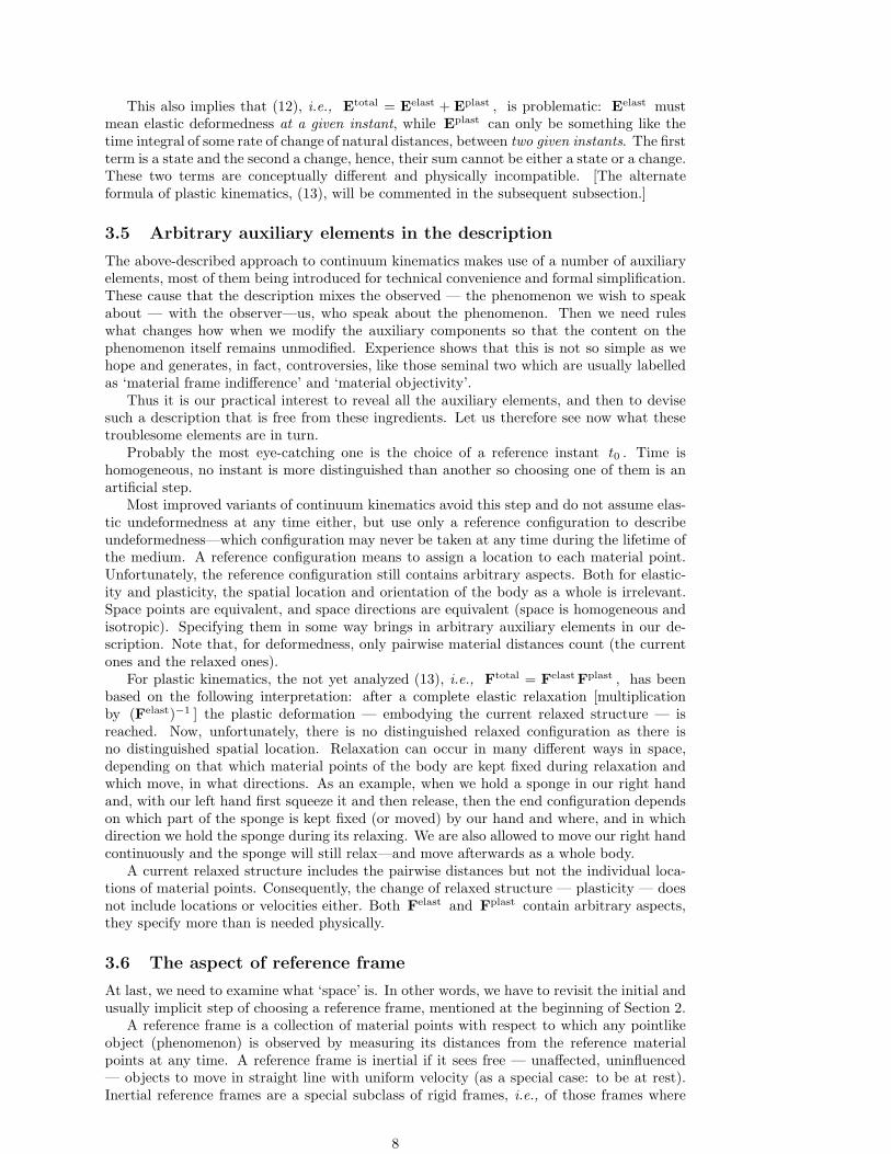
This also implies that (12), i.e., Etotal = Eelast + Eplast , is problematic: Eelast mustmean elastic deformedness at a given instant, while Eplast can only be something like thetime integral of some rate of change of natural distances, between two given instants. The firstterm is a state and the second a change, hence, their sum cannot be either a state or a change.These two terms are conceptually different and physically incompatible. [The alternateformula of plastic kinematics, (13), will be commented in the subsequent subsection.]

3.5 Arbitrary auxiliary elements in the description

The above-described approach to continuum kinematics makes use of a number of auxiliaryelements, most of them being introduced for technical convenience and formal simplification.These cause that the description mixes the observed — the phenomenon we wish to speakabout — with the observer—us, who speak about the phenomenon. Then we need ruleswhat changes how when we modify the auxiliary components so that the content on thephenomenon itself remains unmodified. Experience shows that this is not so simple as wehope and generates, in fact, controversies, like those seminal two which are usually labelledas ‘material frame indifference’ and ‘material objectivity’.

Thus it is our practical interest to reveal all the auxiliary elements, and then to devisesuch a description that is free from these ingredients. Let us therefore see now what thesetroublesome elements are in turn.

Probably the most eye-catching one is the choice of a reference instant t0 . Time ishomogeneous, no instant is more distinguished than another so choosing one of them is anartificial step.

Most improved variants of continuum kinematics avoid this step and do not assume elas-tic undeformedness at any time either, but use only a reference configuration to describeundeformedness—which configuration may never be taken at any time during the lifetime ofthe medium. A reference configuration means to assign a location to each material point.Unfortunately, the reference configuration still contains arbitrary aspects. Both for elastic-ity and plasticity, the spatial location and orientation of the body as a whole is irrelevant.Space points are equivalent, and space directions are equivalent (space is homogeneous andisotropic). Specifying them in some way brings in arbitrary auxiliary elements in our de-scription. Note that, for deformedness, only pairwise material distances count (the currentones and the relaxed ones).

For plastic kinematics, the not yet analyzed (13), i.e., Ftotal = FelastFplast , has beenbased on the following interpretation: after a complete elastic relaxation [multiplicationby (Felast)−1 ] the plastic deformation — embodying the current relaxed structure — isreached. Now, unfortunately, there is no distinguished relaxed configuration as there isno distinguished spatial location. Relaxation can occur in many different ways in space,depending on that which material points of the body are kept fixed during relaxation andwhich move, in what directions. As an example, when we hold a sponge in our right handand, with our left hand first squeeze it and then release, then the end configuration dependson which part of the sponge is kept fixed (or moved) by our hand and where, and in whichdirection we hold the sponge during its relaxing. We are also allowed to move our right handcontinuously and the sponge will still relax—and move afterwards as a whole body.

A current relaxed structure includes the pairwise distances but not the individual loca-tions of material points. Consequently, the change of relaxed structure — plasticity — doesnot include locations or velocities either. Both Felast and Fplast contain arbitrary aspects,they specify more than is needed physically.

3.6 The aspect of reference frame

At last, we need to examine what ‘space’ is. In other words, we have to revisit the initial andusually implicit step of choosing a reference frame, mentioned at the beginning of Section 2.

A reference frame is a collection of material points with respect to which any pointlikeobject (phenomenon) is observed by measuring its distances from the reference materialpoints at any time. A reference frame is inertial if it sees free — unaffected, uninfluenced— objects to move in straight line with uniform velocity (as a special case: to be at rest).Inertial reference frames are a special subclass of rigid frames, i.e., of those frames where

8

the pairwise distances of reference material points are time independent. Nonrigid framesalso find applications.

In the approach to continuum kinematics considered in Section 2, it would be importantto specify what reference frame is used. From a noninertial frame, freely moving bodies areseen to have possess some acceleration or rotation, while to be rest with respect to sucha frame requires some appropriate forces. Therefore, using a noninertial frame brings inartifacts, the auxiliary element of using a reference frame allows the presence of disturbingfeatures which belong to the observer and not to the phenomenon we wish to observe. Least‘harm’ is done by using an inertial reference frame.

Galileo is known to point out first that inertial reference frames are physically equivalent,neither of them is distinguished from the others. His example to explain this was a ship onstill water [26]: if we are in a windowless cabin within the ship, we cannot determine whetherthe ship is at rest with respect to the shore or moves with some uniform velocity to somedirection, no matter what type of physical experiment we perform in the cabin.

Inertial reference frames move uniformly with respect to each other. When changingfrom one to another that moves with relative velocity V with respect to the former, thentime and position are to be transformed as

t′ = t, x′ = x−Vt (30)

according to the Galilean transformation rule, which is applicable in the nonrelativisticregime of relative velocities much smaller than the speed of light. From this, we can read offthat, nonrelativistically, time is absolute as the transformation rule for time is of the formt′ = f(t) . Similarly do we find that space is not absolute since x′ 6= g(x) .

From x′ = g(t,x) = x − Vt it is also clear that, to make space absolute, it must be

combined with time. Forming the four dimensional combination

tx

, the transformation

rule reads(t′

x′

)=

(t

x−Vt

)=

(1 0

−V I

)(tx

)(31)

so the transformation does not lead out of the set of

tx

values, and there is an absolute,

physical, four dimensional quantity (four-vector) behind whose representation in one inertial

frame is

tx

and is

t′

x′

in another.

That space is not absolute is also clear from the fact that, for any reference frame, thereference material points are the space points of that frame, and they indicate the ‘restinglocations’ as seen from that frame. (A side remark: in practice, for a frame we do not fillthe whole world with material points but take only a restricted amount of them, and useinterpolation-extrapolation rules for the other, empty, locations.) Now, if a frame moveswith respect to another then the reference material points — the resting locations — do notrest with respect to the other frame. What is a space point for one frame is a process forthe other one.

This actually coincides with our everyday experience as well. When travelling on a train,our reference frame is fixed to the train: the seats, the window, etc. Even when our drinkspills out of our cup because of a fast breaking of the train, we view this from a viewpointfixed to the train—although the drink wished to continue its inertial motion and it was thetrain that did something noninertial. In the meantime, someone seeing this little accidentfrom the outside, standing on the earth nearby the rail, sees us, the drink and the wholetrain as moving.

There is not one space as ‘the universal background’ of motions. There is one spacetimewhich is the universal background of motions but spaces are relative, they are relative toframes/observers.

Certainly, to take the step of combining space with time has not been easy historically,both because of physical and mathematical aspects. Physically, time is experienced to bedifferent from space in some senses. In parallel, mathematically, geometry originally meanta Euclidean space, and it took much time to gradually realize that geometries other thanEuclidean are also conceptually acceptable—and even relevant.

9

The four dimensional combinations show not a four dimensional Euclidean structure butthe combination of two other structures. One of them is the linear map that takes the time

component t out of

tx

, and the other is a three dimensional Euclidean scalar product

(0x1

)·(

0x2

)= x1 · x2 (32)

for the spacelike combinations

0x

— the ones which have zero timelike component —,

which combinations are actually those invariant under Galilean transformation:

(0x

)′

=

(0

x−V · 0

)=

(0x

). (33)

The time component is absolute, and consequently simultaneity of spacetime points also,and spacelike four-vectors with their scalar product are also absolute.

Historically, only the advent of special relativity helped to rethink the nonrelativisticspace and time ideas as well. That’s why Newton rejected Galileo’s result on the equivalenceof inertial reference frames, and claimed the existence of an absolute space (a distinguishedframe): he could not imagine any other background for his action-at-a-distance forces. Hedidn’t know that absolute simultaneity plus absolute spacetime vectors with Euclidean struc-ture would suffice for this purpose, and, at the same time, would allow to incorporate theequivalence of inertial reference frames, too.

Some years after the birth of special relativity, another important achievement took place:Weyl published such a formalism for spacetime — he established both the nonrelativistic andthe special relativistic version— that does not rely on reference frames [11]. Spacetime pointsand their relationships, i.e., the structures of spacetime, are defined first, then pointlikeobjects are modelled with world lines in spacetime, and reference frames are introduced onlylater, as certain extended objects moving in spacetime.

This approach has gained attention only gradually, was popularized by Arnold, for ex-ample [27] Then, the quite succinct and basic treatment by Weyl was expounded, enrichedand worked out in detail for the purposes of physics by Matolcsi [13, 20].

The frame free spacetime formalism enables us to remove the reference frame, the lastarbitrary auxiliary element to be listed in this Section, from continuum kinematics. Mate-rial objectivity can be viewed directly, without the disturbing technical presence of frames.Also, the question of material frame indifference can be cleanly reworded as the questionof noninertial motion indifference (does some interaction within the material couple to theacceleration, or to the angular velocity of the continuum?). While the present work doesnot intend to contribute directly to the topics of material objectivity and noninertial motionindifference, that questions will also be possible to investigate on the grounds layed downhere in the subsequent Sections: a frame free discussion of kinematics, with all the otherauxiliary ingredients also avoided.

In what follows, let us follow the general methodology of mathematical models for physicalphenomena [28], with all notions introduced as mathematical objects, defined fully mathe-matically, so as not to leave any property obscured or tacitly assumed.

4 Spacetime without reference frames

4.1 Quantities with physical dimension (length, time, etc.)

Units chosen for dimensionful physical quantities — length, time, mass, etc. — are alsoauxiliary elements in a description. Therefore, let us avoid them, too, by utilizing the unitfree approach [MTfeher], where we introduce separate one dimensional oriented real vectorspaces (in short, measure lines) L , T , M for lengths, time intervals and mass values,respectively. A length, for example, is an element ℓ of L , sums of lengths ℓ1 + ℓ2 and realmultiples of lengths αℓ also being elements of L . It will be useful to summarize here howthe unit free treatment gives account of the properties of dimensionful quantities.

10

- Tt1 t2 t3

|| |

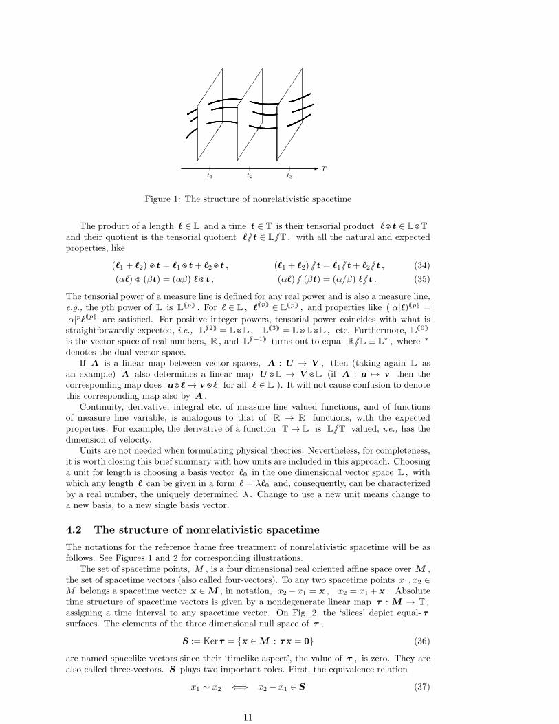
Figure 1: The structure of nonrelativistic spacetime

The product of a length ℓ ∈ L and a time t ∈ T is their tensorial product ℓ⊗t ∈ L⊗T

and their quotient is the tensorial quotient ℓ//t ∈ L//T , with all the natural and expectedproperties, like

(ℓ1 + ℓ2) ⊗t = ℓ1 ⊗t + ℓ2 ⊗t , (ℓ1 + ℓ2) //t = ℓ1//t+ ℓ2//t , (34)

(αℓ) ⊗ (βt) = (αβ) ℓ⊗t , (αℓ) // (βt) = (α/β) ℓ//t . (35)

The tensorial power of a measure line is defined for any real power and is also a measure line,e.g., the pth power of L is L

((p)) . For ℓ ∈ L , ℓ((p)) ∈ L((p)) , and properties like (|α|ℓ)((p)) =

|α|pℓ((p)) are satisfied. For positive integer powers, tensorial power coincides with what isstraightforwardly expected, i.e., L

((2)) = L⊗L , L((3)) = L⊗L⊗L , etc. Furthermore, L

((0))

is the vector space of real numbers, R , and L((−1)) turns out to equal R//L ≡ L

∗ , where ∗

denotes the dual vector space.If A is a linear map between vector spaces, A : U → V , then (taking again L as

an example) A also determines a linear map U ⊗L → V ⊗L (if A : u 7→ v then thecorresponding map does u⊗ℓ 7→ v ⊗ℓ for all ℓ ∈ L ). It will not cause confusion to denotethis corresponding map also by A .

Continuity, derivative, integral etc. of measure line valued functions, and of functionsof measure line variable, is analogous to that of R → R functions, with the expectedproperties. For example, the derivative of a function T → L is L//T valued, i.e., has thedimension of velocity.

Units are not needed when formulating physical theories. Nevertheless, for completeness,it is worth closing this brief summary with how units are included in this approach. Choosinga unit for length is choosing a basis vector ℓ0 in the one dimensional vector space L , withwhich any length ℓ can be given in a form ℓ = λℓ0 and, consequently, can be characterizedby a real number, the uniquely determined λ . Change to use a new unit means change toa new basis, to a new single basis vector.

4.2 The structure of nonrelativistic spacetime

The notations for the reference frame free treatment of nonrelativistic spacetime will be asfollows. See Figures 1 and 2 for corresponding illustrations.

The set of spacetime points, M , is a four dimensional real oriented affine space over M ,the set of spacetime vectors (also called four-vectors). To any two spacetime points x1, x2 ∈M belongs a spacetime vector x ∈ M , in notation, x2 − x1 = x , x2 = x1 +x . Absolutetime structure of spacetime vectors is given by a nondegenerate linear map τ : M → T ,assigning a time interval to any spacetime vector. On Fig. 2, the ‘slices’ depict equal- τsurfaces. The elements of the three dimensional null space of τ ,

S := Kerτ = x ∈ M : τx = 0 (36)

are named spacelike vectors since their ‘timelike aspect’, the value of τ , is zero. They arealso called three-vectors. S plays two important roles. First, the equivalence relation

x1 ∼ x2 ⇐⇒ x2 − x1 ∈ S (37)

11

qAAK :p p pPPP qp p p pQQQsp p p

0

ℓϕ

-T

q

−t 0 t

| |

S

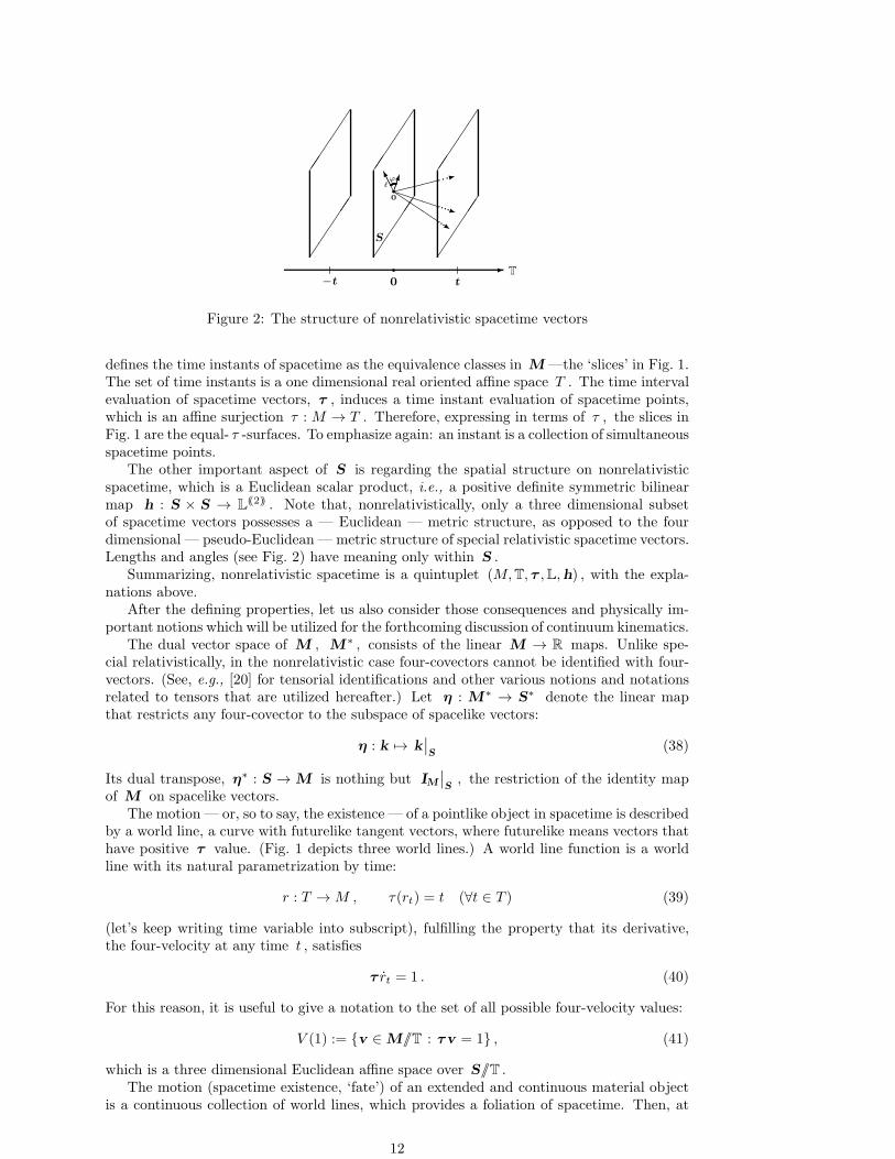
Figure 2: The structure of nonrelativistic spacetime vectors

defines the time instants of spacetime as the equivalence classes in M —the ‘slices’ in Fig. 1.The set of time instants is a one dimensional real oriented affine space T . The time intervalevaluation of spacetime vectors, τ , induces a time instant evaluation of spacetime points,which is an affine surjection τ : M → T . Therefore, expressing in terms of τ , the slices inFig. 1 are the equal- τ -surfaces. To emphasize again: an instant is a collection of simultaneousspacetime points.

The other important aspect of S is regarding the spatial structure on nonrelativisticspacetime, which is a Euclidean scalar product, i.e., a positive definite symmetric bilinearmap h : S × S → L

((2)) . Note that, nonrelativistically, only a three dimensional subsetof spacetime vectors possesses a — Euclidean — metric structure, as opposed to the fourdimensional — pseudo-Euclidean — metric structure of special relativistic spacetime vectors.Lengths and angles (see Fig. 2) have meaning only within S .

Summarizing, nonrelativistic spacetime is a quintuplet (M,T, τ ,L,h) , with the expla-nations above.

After the defining properties, let us also consider those consequences and physically im-portant notions which will be utilized for the forthcoming discussion of continuum kinematics.

The dual vector space of M , M∗ , consists of the linear M → R maps. Unlike spe-cial relativistically, in the nonrelativistic case four-covectors cannot be identified with four-vectors. (See, e.g., [20] for tensorial identifications and other various notions and notationsrelated to tensors that are utilized hereafter.) Let η : M∗ → S∗ denote the linear mapthat restricts any four-covector to the subspace of spacelike vectors:

η : k 7→ k∣∣S

(38)

Its dual transpose, η∗ : S → M is nothing but IM∣∣S, the restriction of the identity map

of M on spacelike vectors.The motion — or, so to say, the existence — of a pointlike object in spacetime is described

by a world line, a curve with futurelike tangent vectors, where futurelike means vectors thathave positive τ value. (Fig. 1 depicts three world lines.) A world line function is a worldline with its natural parametrization by time:

r : T → M , τ(rt) = t (∀t ∈ T ) (39)

(let’s keep writing time variable into subscript), fulfilling the property that its derivative,the four-velocity at any time t , satisfies

τ rt = 1 . (40)

For this reason, it is useful to give a notation to the set of all possible four-velocity values:

V (1) := v ∈ M//T : τv = 1 , (41)

which is a three dimensional Euclidean affine space over S//T .The motion (spacetime existence, ‘fate’) of an extended and continuous material object

is a continuous collection of world lines, which provides a foliation of spacetime. Then, at

12

any spacetime point, we have a four-velocity value, which is the derivative there of the worldline function that goes through that spacetime point. Thus a four-velocity field on spacetimecan be read off. The opposite way is also possible for giving a motion of a continuum, whenwe start with a — smooth enough — four-velocity field on spacetime and determine themaximal integral curves of that four-vector field, which integral curves will be the worldlines of the material body.

Any reference frame or spacetime observer is also such a possible continuum motionin spacetime. The space points of an observer are the world lines. Especially, an inertialobserver admits world lines that are parallel straight lines with a single prescribed four-velocity value as their tangent vector that is constant along each world line and is the samevalue for all world lines.

A more general and also important family of observers is the rigid observers, where thedistance of any two space points of the observer are time independent. Note that an instantis a spacelike three dimensional affine subspace in spacetime which intersects each world line,each futurelike curve at exactly one spacetime point, and the distance of two space points ofan observer at a time is the Euclidean length of the two such intersection points. When thisdistance is the same for all times for this given pair of world lines, and if all such pairwisedistances are time independent then the observer is called rigid.

The space of a rigid observer proves to be a three dimensional Euclidean affine space. Fornonrigid observers, not even a time independent Riemann metric structure can be found, ingeneral, so we are left with only a smooth manifold.

Calculus of functions defined on spacetime is similar to that of defined on R4 , though

some differences emerge because R4 is a Euclidean vector space while, on M , which lies

under M , the structures τ and h are more tricky. The spacetime derivative of a scalarfield f : M → R , denoted by f ⊗D (to be systematic, derivatives will always be writtenindicating the correct tensorial order) takes an M∗ value at each spacetime point. It ex-presses how fast f changes in a spacetime direction. The restriction η(f ⊗D) = (f ⊗D)η∗ ,denoted hereafter by f ⊗∇ , tells how fast f changes in spacelike directions. Hence, ∇ isthe spatial derivative, which proves thus to be an absolute (frame independent) operation,although absolute space does not exist but spaces depend on observers. The explanation isthat spacelikeness is absolute and this is enough for spatial derivative.

The derivative of a four-vector field f : M → M is M ⊗M∗ valued at every point, thetrace of which is the four-divergence. In parallel, the spatial derivative q⊗∇ of a three-vector field or spacelike vector field q : M → S is S⊗S∗ valued, the trace of which is thethree-divergence. On the other side, the spatial derivative of an M → S∗ three-covectorfield is S∗ ⊗S∗ , whose the antisymmetric part leads to the curl, ∇× , of the three-covectorfield.

An important special case is the derivative of a four-velocity field v : M → V (1) ⊂M//T . Since the difference of any two elements of V (1) is spacelike, differences of four-velocities are always spacelike. Consequently, v ⊗D and v ⊗∇ are not only M//T⊗M∗

and M//T⊗S∗ valued, respectively, but S//T⊗M∗ , resp. S//T⊗S∗ valued. Therefore,the three-divergence of a four-velocity field is automatically meaningful, while the curl onlyafter utilizing the identification S ≡ S∗ ⊗L

((2)) provided by h .

5 The material manifold of solids

Let the mathematical model for a continuum be a three dimensional simply connectedcomplete smooth manifold C . Its tangent space at a material point, an element P of C ,is TP (C) . The differential map of a smooth mapping φ from C to an arbitrary smooth

manifold M at a point P is a linear map TP (C) → Tφ(P ) (M) , denoted by (φ⊗ ∇)(P ) .

Henceforth, overtilde will indicate material vectors, covectors, tensors etc., i.e., objects re-lated to the tangent spaces of C (i.e., referring to material directions) to make a distinctionto vectors etc. related toS of spacelike spacetime vectors — spatial directions — (as well asto quantities related to M , though these latter will occur only infrequently in what follows).

A motion or spacetime process of such a body is given by assigning a world line functionr to each material point P in a smooth enough way. Thence, at a time t , point P is atspacetime point rt(P ) . For a fixed t , P 7→ rt(P ) is a mapping from C to t — let’s recall

13

that a t is a Euclidean affine space, a three dimensional ‘slice’ within spacetime —, with itsdifferential map or Jacobian map at P

Jt(P ) = (rt ⊗ ∇)(P ) . (42)

This Jacobian is the frame free & reference time free & reference configuration free general-ization of the deformation gradient.

The four-velocity of a material point P at a time t is

vt(P ) = rt(P ) . (43)

For convenience, hereafter let us not distinguish in notation functions defined on C (La-grangian description; e.g., vt ) from their Eulerian-like spacetime counterpart (their compo-sition with r−1

t for each t ; e.g., vt r−1t ). It is easy to check that, for a function f defined

on spacetime, the comoving derivative f is to be introduced as (f ⊗D)v so that it be inaccord with the overdot of Lagrangian variabled functions.

Using the chain rule of differentiation of composite functions,

Lt := vt⊗∇ (44)

can be expressed with Jt as

Lt = JtJ−1t . (45)

At any instant t , the current distance of two material points P,Q is the distance of thetwo spacetime points rt(P ), rt(Q) where the two material points stay at t ,

dt(P,Q) = ‖rt(Q)− rt(P )‖h . (46)

This induces a Riemann metric tensor on C , which proves to be

ht = J∗

t hJt , ht(P ) : TP (C)× TP (C) → L((2)) . (47)

Actually, the following three characterizations of distance relationships are equivalent ona Riemann manifold: 1) lengths of curves, 2) distances of pairs of points (defined as thelength of the shortest, geodesic, curve between the two points), 3) the metric tensor. Thethird choice uses a local quantity while the other two are nonlocal characterizations so it isfavourable to work in terms of the metric tensor.

So far we haven’t restricted our discussion to elastic solids. To make this step, let usrealize the physical ideas put forward in Sects. 3.3 and 3.6 by adding to our model of thecontinuum a mathematical object that expresses the relaxed/natural distances of pairs ofmaterial points. This means that we furnish our material manifold with a natural/relaxedRiemann metric tensor g . In general, this metric is different from the currently realizedmetric ht . In other words, in general the body is not relaxed, it is not undeformed, noteven within some local neighbourhood. It might be considered as a ‘blessed moment’ whenthe two metrics coincide.

Nevertheless, we require something from the relaxed metric: that, under appropriatecircumstances, the current metric could evolve into the relaxed metric: that it is possible tobring the body into relaxed state, even within a finite time interval, by some finite later timet , via some motion r that would connect smoothly to the current motion rt of the materialand would continue in such a way that the distances realized at t coincide with the relaxedones for the whole body. (In short: The relaxed metric must be realizable as a current metricat some time t . A solid must have the ability to relax.) In the language of metrics, this is

expressed as ht = g . Writing this in terms of rt and its gradient Jt = rt ⊗∇ reads

J∗

t hJt = g , (48)

which tells that rt establishes an isometry, a metric preserving diffeomorphism, between Cas a Riemann manifold with metric g and t as a Riemann manifold with metric h .

Now, we know that t is actually a Euclidean affine space and, hence, a flat Riemannmanifold (i.e., having zero Riemann curvature tensor). Due to a theorem (see eg. [29]), a

14

Riemann manifold is isometric to a flat one iff it is flat. Therefore, the relaxed structure onC is required to be a flat Riemann metric.

This condition can be further reformulated in a technically more convenient way. Namely,C being three dimensional, not only its Riemann tensor determines its Ricci tensor but theRicci tensor also determines the Riemann tensor (one proof of this can be based on p88of [30]). Consequently, the requirement of flatness is equivalent to the zeroness of the Riccitensor. To summarize, the physical expectations dictate the relaxed structure of a solid bodyto be a Ricci-flat Riemann metric.

6 Elastic kinematics

6.1 Elastic shape

In the light of Sect. 3.3, elastic kinematics needs a quantity that expresses how the currentdistances — on C , the current metric ht , — differ from the relaxed distances — on C ,from the relaxed metric g . Or, in terms of spatial spacetime tensors, the current distances— on t , h — are to be compared to the relaxed distances — on t , to

gt :=(J−1t

)∗g J−1

t . (49)

Both ht and g are TP (C) →[TP (C) /L((2))

]∗type linear maps, and both h and gt are

S →[S/L((2))

]∗type maps.

It is also instructive to remark that it would be advantageous if the elastic kinematicquantity agreed with the Cauchy strain in the regime of small deformedness. We can formu-late its definition (21) in the frame free approach via its evolution equation as

E in.Cauchy =1

2

(L+ h−1L∗h

)=

1

2

(L+ L+

)= LS , (50)

where the appearance of h is unavoidable and the h -adjoint

L+ := h−1L∗h (51)

of L = v ⊗∇ must be used because L is an S → S//T tensor, and its dual transpose, aS∗ → S∗//T tensor cannot be added to it, except when h : S →

(S//L((2))

)∗is also inserted

as appropriate. The resulting E in.Cauchy is S → S valued, and is h -symmetric.Incidentally, the reinterpretation of the traditional Cauchy strain would require to involve

the Jacobian J as well, since the material gradient of velocity maps from TP (C) to S soit can be combined with its dual transpose only when an appropriate map between TP (C)and S is also made use of. Note that the Jacobian tensor J (the spacetime consistentgeneralization of the deformation gradient) can never be ‘close to the identity tensor’ sinceit connects different vector spaces so the traditional Cauchy strain would become a rathercomplicated object when seen in the frame free & reference time free & reference configurationfree way. In what follows, let us use (for comparison purposes and for checking the smalldeformedness regime) only the inertial version, which is a simple and clear object.

Now, having seen that from what vector space and to what vector space the currentmetric tensor and the relaxed metric tensor map, mathematics allows to compose these twolinear maps only in the combination

At := g−1t h (52)

as the spacelike spacetime tensorial version, and as

At = J−1t AtJt = g−1 ht , (53)

the material equivalent of At . It is easy to check that At is an h -symmetric S → S

tensor, while At is a g -symmetric TP (C) → TP (C) type tensor.

If the material is in its relaxed state, ht = g , gt = h , then At(P ) = ITP(C) , At = IS .

This seems to indicate that we have introduced not a deformedness (a reinterpreted strain)but a reinterpreted deformation. We can call it elastic shape tensor.

15

It is possible to derive the time evolution equation of the elastic shape tensor. With (45)and (51), it is in fact straightforward to find

A = LA+AL+ . (54)

Comparing this with (18) shows that what we have at hand is actually the frame free &reference time free & reference configuration free generalization of the left Cauchy-Greendeformation tensor. Its material version is, therefore, the reformed version of the rightCauchy-Green tensor.

Based on the definition of A , one can show that

det√At =

√detAt =

√|h|√|gt|

=

√∣∣ht

∣∣√|g |

, (55)

where |√· | denotes the volume form that a Riemann metric defines. This quantity is,therefore, the ratio of the current volume and the relaxed volume of a small amount ofmaterial. This formula is in accord with (the square of) equation (16).

For small deformedness, which can already be formulated as At ≈ IS , i.e., their dif-ference being much smaller than IS in tensorial norm, the rate equation (54) becomes, inleading order of At − IS ,

(At − IS.

) ≈ 2LS . (56)

Comparing this with (50) shows that we have found the link

12 (At − IS) ≈ E in. Cauchy (At − IS ≪ IS) (57)

with the Cauchy deformedness (i.e., from any given small initial deformedness, the twoevolve the same way in leading order).

6.2 Deformedness

For deformedness itself, we are interested in such a function of A that, for At ≈ IS , isapproximately 1

2 (At − IS) . This is actually a large amount of freedom but we already havea geometrically distinguished desire as well: that the trace of the deformedness tensor shouldexpress the volumetric aspect of elastic expandedness and its deviatoric part the constant–volume deformednesses. In the light of Sect. 3.2 and formula (55), it is not surprising to findthat this can be accomplished by the Hencky type choice:

D := ln√A =

1

2lnA , =⇒ trD = ln

√detA . (58)

As such, D also satisfies the wish raised in Sect. 3.2 that our deformedness quantity shoulddiverge both for infinite compression and for infinite extension.

In parallel, it is easy to see that

D ≈ 12 (A− IS) ≈ E in.Cauchy (whenever D ≪ IS) . (59)

Although the present work concentrates on the kinematic issues, some arguments canalready be added on the advantage of the Hencky deformedness in constitutive relations. Onthe theoretical side, one can show — the simple details of the calculation omitted here —that, if the Cauchy stress σ can be derived from a quadratic elastic potential U(D) of anisotropic solid as

σ = ρdU

dD(60)

( ρ denoting density) then its mechanical power, trσL , is found to be simply

trσL = ρU . (61)

16

This is exactly the expression that is the natural one in connection with a continuity equationfor energy. Hence, this simple example suggests that the variable D behaves distinguishedlyfrom energetic and, consequently, thermodynamic point of view.

In parallel, it has already been mentioned in Sect. 3.1 that the Hencky choice is favouredby experiments in the linear regime of elastic stress-deformedness relation, as well as forthe role of the variable of nonlinear elastic constitutive relations. Naturally, these aspectsrequire extensive further investigation to collect a satisfactory amount of knowledge on thesubject.

6.3 The compatibility condition

We have seen, in Sect. 5, that the relaxed metric must be Ricci-flat. This imposes a restrictionon A . Working with the spacelike spacetime tensorial version gt , its Ricci tensor can beexpressed in a coordinate free version of the usual coordinate formula [30] since the manifold,t , on which gt is given is a Euclidean affine space:

RRiccit = ∇ · Γt − (tr1,3Γt)⊗∇+ (tr1,3Γt)Γt − tr1,3(ΓtΓt) , (62)

where the Christoffel tensor is

Γt =12 g

−1t

[gt ⊗∇+ (gt ⊗∇)T2,3 −∇⊗gt

]. (63)

As gt= hA−1

t [cf. (52)], the requirement RRiccit = 0 can be reformulated as a condition

on At . Omitting the rather lengthy details of the calculation [31], one can obtain

tr1,5;3,4[A−1

⊗A−1 (A⊗∇) (A⊗∇)]+ 2hA−1 tr1,2

[Ah−1 (∇⊗∇⊗A)

]A−1+

+2h tr2,3[A−1

⊗ (∇ ·A)h−1 (∇⊗A)]A−1 − 2hA−1 tr2,4

[(A⊗∇⊗∇)h−1

]+

+2tr1,4;3,5[A−1

⊗A−1 (A⊗∇) (A⊗∇)]+ tr1,2;3,5

[A−1 (A⊗∇) (A⊗∇) ⊗A−1

]−

−2hA−1 tr2,5;3,6[(A⊗∇)Ah−1 (∇⊗A) ⊗A−1

]A−1+ (64)

+2tr2,4[(∇⊗A)A−1 (A⊗∇)

]A−1 − 3tr2,6;3,5

[(∇⊗A)A−1 (A⊗∇) ⊗A−1

]−

−2 [∇⊗ (∇ ·A)]A−1 − h tr3,4;2,5[A−1

⊗A−1 (A⊗∇)Ah−1 (∇⊗A)]A−1+

+2tr1,2[A−1 (A⊗∇⊗∇)

]− 2hA−1 tr2,4;3,5

[(A⊗∇) ⊗h−1 (∇⊗A)

]A−1 = 0 .

This complicated nonlinear equation is to be satisfied by A . ‘Fortunately’, it is enough tosatisfy it at a given time and then the time evolution equation will ensure that at later timesit still holds true.

In the small deformedness regime, the leading order term of this condition turns out tobe extremely simple:

∇×D ×∇+ (higher order terms) = 0 . (65)

In fact, this is what we would expect even without calculation, as being the spacetime versionof the Saint-Venant compatibility condition (25). Formula (64) is, hence, the compatibilitycondition for finite deformedness. Nevertheless, the derivation of (65) from (64) proceeds asfollows. In (64), there are two types of terms: either containing a second derivative of A orcontaining the product of two first derivatives of A. Assuming that A− IS is small even inthe sense that the product of two first derivatives is much smaller than a second derivative,we can keep in (64) only the terms with a second derivative:

2hA−1 tr1,2[Ah−1 (∇⊗∇⊗A)

]A−1 − 2hA−1 tr2,4

[(A⊗∇⊗∇)h−1

]− (66)

−2 [∇⊗ (∇ ·A)]A−1 + 2tr1,2[A−1 (A⊗∇⊗∇)

]≈ 0 .

Inserting A ≈ IS directly as well yields

2h tr1,2[h−1 (∇⊗∇⊗A)

]− 2h tr2,4

[(A⊗∇⊗∇)h−1

]− (67)

−2 [∇⊗ (∇ ·A)] + 2tr1,2 [(A⊗∇⊗∇)] ≈ 0 .

17

This formula is already linear in A . Substituting (59) into it, and after simple technicalsteps, we arrive at (65).

For technical purposes, it would be advantageous to be able to characterize those A

which satisfy the compatibility condition in some alternative way that is simpler than thecondition itself. An idea to do this is as follows. The relaxed metric g is flat so, for any t , itcan be brought into isometry with h , the metric of any t . Let us choose such an isometry

rt : C → t (∀t) . (68)

It looks like a motion of the continuum in spacetime but its is not the true motion but onlyan auxiliary ‘pseudo-motion’. It can be chosen fairly arbitrarily: actually, it is arbitrary upto the isometries of an Euclidean affine space, which are the translations and rotations. Informula, any other such isometry r′t is related to rt as

r′t = Rt (rt − ot) + ot (69)

with an arbitrary—world line function-like—function ot (carrying the translation freedom)and an arbitrary h -orthogonal tensor valued function Rt , which embodies the rotationdegree of freedom, and rotates around ot . For the Jacobian of the auxiliary pseudo-motion,

Jt := rt ⊗∇ , (70)

a part of the freedom disappears and only the rotation remains:

J′

t = Rt Jt . (71)

All in all, this auxiliary pseudo-motion is introduced not for any principal role but as atechnical aid.

The property that it is an isometry between C with g and t with h provides therelationship

g = J∗

t hJt (72)

between the two metrics, and, similarly, substituting this into (52) using (53) yields

At = Jt Jt−1h−1

(Jt

−1)∗J∗

t h . (73)

Let us observe that

Jt Jt−1 =

(rt ⊗∇

)(rt ⊗ ∇

)−1=

(rt rt−1

)⊗∇ = qt ⊗∇ (74)

with

qt := rt rt−1 − It , (75)

a spacelike four-vector field on t , where It is the identity affine map of the affine space t .In terms of this vector field,

At = (qt ⊗∇) (qt ⊗∇)+. (76)

Therefore, any At allowed by the compatibility condition can be given in terms of a spacelikevector field qt on t . This qt is not unique but carries the arbitrarinesses that hold for rt .A qt can be called a vector potential of elastic shape.

We are actually more familiar with this qt than it seems at first sight. Indeed, when

qt ⊗∇ ≈ IS (77)

(in the sense as for the above approximations) then

At ≈ IS (78)

so we are in the small deformedness regime, and, keeping one more order,

At ≈ IS + 2 (qt ⊗∇− IS)S , or Dt ≈ (qt ⊗∇− IS)

S . (79)

Let us now take a look at (29) to realize that qt is nothing but the finite deformednessgeneralization and frame & etc. free generalization of the Cauchy potential.

18

7 Plastic kinematics

As analyzed in Sect. 3.4, plasticity is a situation when the natural, relaxed, structure ofa solid becomes time dependent. Accordingly, plastic kinematics must be described by sucha quantity that measures the rate of change of this time dependence.

On the material manifold, this is expressed by gt —or, equivalently, by(g−1t

.). On space-

time, the corresponding quantity, Jt(g−1t

.)J∗t , provides the additional term that appears

when (54) is generalized to time dependent g :

At =(Jt g

−1t J∗

t h.)= LtAt +AtL

+t −Wt (80)

with

Wt := −Jt(g−1t

.)J∗

t h = Jt g−1t gt g

−1t J∗

t h . (81)

W is a state variable that expresses plastic change rate, and can be named the metricchange tensor. Therefore, in a continuum theory involving plastic phenomena, the completeset of dynamical and constitutive equations must contain an equation that determines thecurrent value of W as a function of other quantities of the continuum. For example, W

may be given as a function of the stress tensor. This function may be nonzero only when astress value, e.g., the shear stress, exceeds a critical value.

The form of this W -determining function is limited by the requirement that W mustbe such that the natural metric structure g t remains Ricci-flat at any time t. This followsfrom the physical expectation that a sudden unloading should stop plastic changes, it shouldstop the change of the natural metric and— in case of zero volume forces —bring the materialto an elastically nondeformed state, bring the current metric to the natural one.

Bearing in mind the complicated form of the compatibility condition (64), to ensurethat the time dependent natural metric stays Ricci-flat is a rather strong restriction on W

mathematically. On the other side, physically it is very valuable since many candidatesfor the W -determining function that seem reasonable for small deformations may fail toadmit a satisfying finite deformation generalization. The strong requirement helps to findphysically admissible models by allowing only a rather limited range of choices.

The two widely used formulas for plastic kinematics, Ftotal = FelastFplast and Etotal =Eelast+Eplast [appeared in Sect. 2 under (13) resp. (12), and already discussed in Sects. 3.4–3.5] can be viewed from the kinematic picture presented here as follows.

Let us rewrite (74) as

J = r⊗ ∇ = (q⊗∇)(r⊗∇

)= (q⊗∇) J (82)

The Jacobian tensor J has already been found to be the spacetime compatible generalizationof the deformation gradient F = Ftotal . Furthermore, the pseudo-motion r is a mapping ofthe relaxed metric structure into spacetime at any instant so it can be ‘interpreted’ (pseudo-

interpreted) as a ‘motion of relaxed positions’. In this sense, r⊗∇ = J is the incarnationof Fplast . Finally, q⊗∇ has been seen to be related to the elastic shape tensor A —compare (76) with the usual formula U2

L = Felast (Felast)T of Sect. 2 and recall that U2L is

the traditional counterpart of A . Hence, q⊗∇ embodies Felast , and thus the relationshipbetween Ftotal = FelastFplast and (82) becomes clear.

It is also apparent that the unphysical arbitrarinesses of Felast and Fplast , pointed outin Sect. 3.5, appear here as the unphysical arbitrarinesses in the pseudo-motion r and inthe related quantities (J and q ).

Next, let us investigate (80) in the regime of small elastic deformedness. (Note that it hasno meaning to consider ‘small plastic deformedness’ because there is no plastic deformed-ness/deformation/strain quantity as a state variable.) In the leading order of small A−IS ,(80) simplifies to

2Dt ≈ Lt + L+t + Jt

(g−1t

.)J∗

t h = (vt⊗∇) + h−1 (∇⊗vt)h+ Jt

(g−1t

.)J∗

t h , (83)

19

which can be rearranged as

1

2

[(vt

⊗∇)J−1t + h−1(J∗

t )−1

(∇⊗vt

)h]≈ Dt − Jt

(g−1t

.)J∗

t h . (84)

Then, let [t1, t2] be a time interval during which J changes only a little:

J(t′)J(t)−1 ≈ IS (∀t, t′ ∈ [t1, t2]) . (85)

Then we can replace J with Jt1 , for example. Integrating in time over [t1, t2] at a fixedmaterial point, and noting that

∫ t2

t1

v =

∫ t2

t1

r = rt2 − rt1 =: ∆r , (86)

we obtain

1

2

[(∆r⊗ ∇

)J−1t1

+ h−1(J∗

t1

)−1(∇⊗∆r)h]≈ ∆D − Jt1

[∫ t2

t1

(g−1t

.)]J∗

t1h

≈ ∆D − Jt1

[g−1t2

− g−1t1

]J∗

t1h ≈ ∆D +∆

(−J g

−1J∗h

)(87)

(where, again, ∆ means changes between t1 and t2 ). On the rightmost hand side, ∆D

is the change of elastic deformedness and the second term expresses purely plastic changes.Therefore, we have reached a formula that embodies Etotal = Eelast +Eplast .

Now, the formalism in Sect. 2 suggests Etotal be some realization of

1

2

[(∆u⊗∇

X

)“+”

(∇

X⊗∆u

)](88)

on the leftmost hand side of (87). However, it has no meaning that Jt1 is approximatelyidentity because Jt1(P ) : TP (C) → S connects different vector spaces, between which thereis no identity map. Only taking t1 as a reference time — and thus choosing an identificationbetween TP (C) and S — enables one to transform Jt1 into the quantities which measurechanges with respect to the reference time. The same step is needed to give a meaningto the addition in (88), too, since an S⊗TP (C)∗ tensor and a TP (C)∗ ⊗S tensor cannotbe added—that’s why the + in (88) is put within quotation marks. Furthermore, ∆u isdefined only with respect to a reference frame. Without reference elements and artificialidentification, (88) is not meaningful and, for a Etotal quantity, one has to be content withthe leftmost side of (87).

8 Summary

The paper has emphasized and elaborated the following points.1. Continuum kinematics must avoid the use of auxiliary elements like reference frame,

reference time and reference configuration, which cause that the observed gets mixedwith the observer and unphysical artefacts emerge in the description.

2. If working solely with material manifold based quantities, one cannot give account ofthe inertial-noninertial aspects of the motion/flow of the continuum.

3. By working on spacetime, one is able to define continuum kinematics without anyauxiliary reference elements, and the inertial-noninertial aspects are properly included.The question of material frame indifference is clarified as the question of noninertialmotion indifference.

4. The spacetime generalization of the deformation gradient is the gradient of the systemof material world lines, which exists for solids, liquids and gases each.

5. Restricting ourselves to solids, the kinematic quantity for elasticity is not to be a two-point function which expresses a change but to be a one-point function, i.e., a statevariable, to express a state: the deviation of the currently realized metric in spacetimefrom the natural metric of the solid.

The natural metric is to which the solid relaxes when unloaded. It follows that thenatural metric must have zero Riemann curvature tensor and zero Ricci tensor. Thisrequirement is the ‘finite deformation compatibility condition’.

20

6. This elastic deformedness quantity evolves in time via a rate equation. The solution ofthis differential equation is fixed by, for example, an initial condition, which, in manycases, cannot be chosen zero.

(A side remark: because of the generally nonzero initial condition, the Cesaro–Volterraformula for small deformations cannot give the displacement since a reference time ina reference frame but rather a vectorial potential-like solution of the Saint-Venantcompatibility condition.)

7. More closely, the natural quantity comparing the current metric and the natural metricturns out to be, in some respect, the spacetime generalization of the left Cauchy-Greendeformation tensor. From this elastic shape tensor, the elastic deformedness tensoris defined as a spacetime analogue of the left Hencky strain, which is kinematicallydistinguished by that its trace expresses volumetric expansion and its deviatoric partthe shear degrees of freedom.

8. Plasticity is a phenomenon when the natural metric structure of the solid changes. Inthe rate equation for the elastic shape tensor, the term emerging for nonzero changerate of the natural metric is to be provided by a plastic constitutive equation, in sucha way that the compatibility condition is preserved by the rate equation.

9. No “elastic deformation gradient” and no “plastic deformation gradient” can be de-fined. The typically used additive or multiplicative rules Etotal = Eelast +Eplast andFtotal = FelastFplast for ‘elastic and plastic deformation’, resp. ‘elastic and plastic de-formation gradient’ fail to carry an objective, i.e., free-of-auxiliary-reference-elementsmeaning.

9 Acknowledgement

The authors thank J. M. Martın-Garcıa for his help in using the xAct software packages.The work was supported by the grant OTKA K81161.

References

[1] Chiara de Fabritiis and P. M. Mariano. Geometry of ineractions in complex bodies.Journal of Geometry and Physics, 54:300–323, 2005.

[2] P. M. Mariano. Geometry and balance of hyperstresses. Rendiconti dei Lincei Matem-atica Applicata, 18:311–331, 2007.

[3] A. Yavari, J. E. Marsden, and M. Ortiz. On spatial and material covariant balance lawsin elasticity. Journal of mathematical physics, 47:042903, 2006.

[4] T. Matolcsi and P. Van. Can material time derivative be objective? Physics Letters A,353:109–112, 2006. math-ph/0510037.

[5] A. I. Murdoch. On criticism of the nature of objectivity in classical continuum physics.Continuum Mechanics and Thermodynamics, 17:135–148, 2005.

[6] M. Frewer. More clarity on the concept of material frame-indifference on classical con-tinuum mechanics. Acta Mechanica, 202:213–246, 2009.

[7] W. Noll. Space-time structures in classical mechanics. In The foundations of mechanicsand thermodynamics (Selected papers by Walter Noll), pages 204–210. Springer Ver-lag, Berlin-Heidelberg-New York, 1974. originally: pp28-34, Delaware Seminar in theFoudnations of Physics, Berlin-Heidelberg-New York, Springer, 1967.

[8] W. Noll. Five contributions to natural philosophy. 2004.www.math.cmu.edu/∼wn0g/noll/FC.pdf.

[9] W. Noll and B. Seguin. Basic concepts of thermomechanics. Journal of Elasticity,101:791–858121–151, 2010.

21

[10] W. Noll. A frame free formulation of elasticity. Journal of Elasticity, 83:291–307, 2006.

[11] H. Weyl. Raum-Zeit-Matterie. Julius Springer, Berlin, 1918. in German.

[12] P. Havas. Four-dimensional formulations of Newtonian mechanics and their relationto the special and the general theory of relativity. Reviews of Modern Physics, pages938–965, 1964.

[13] T. Matolcsi. A Concept of Mathematical Physics: Models for SpaceTime. AkademiaiKiado (Publishing House of the Hungarian Academy of Sciences), Budapest, 1984.

[14] C. Truesdell and W. Noll. The Non-Linear Field Theories of Mechanics. SpringerVerlag, Berlin-Heidelberg-New York, 1965. Handbuch der Physik, III/3.

[15] P. Haupt. Continuum Mechanics and Theory of Materials. Springer Verlag, Berlin-Heidelberg-New York, 2nd edition, 2000.

[16] A. Bertram. Elasticity and plasticity of large deformations (An introduction). Springer,2005.

[17] A. DiCarlo. Surface and bulk growth unified. In P. Steinmann and G. A. Maugin,editors, Mechanics of material forces, pages 53–64. Springer, 2005.

[18] M. Epstein. On material evolution laws. In G.A. Maugin, editor, Geometry, continuaand microstructure, pages 1–9. Hermann, Paris, 1999.

[19] M. de Leon. A geometrical description of media with microstructure: uniformity andhomogeneity. pages 11–20. Hermann, Amsterdam-etc., 2005.

[20] T. Matolcsi. Spacetime Without Reference Frames. Akademiai Kiado Publishing Houseof the Hungarian Academy of Sciences), Budapest, 1993.

[21] C.O. Horgan and J.G. Murphy. A generalization of Hencky’s strain-energy densityto model the large deformations of slightly compressible solid rubbers. Mechanics ofMaterials, 79:943–950, 2009.

[22] J. Plesek and A. Kruisova. Formulation, validation and numerical procedures forHencky’s elasticity model. Computers and Structures, 84:1141–1150, 2006.

[23] K. Matsuki and K. Takeuchi. Three-dimensional in situ stress determination by anelasticstrain recovery of a rock core. Int. J. Rock Mech. Min. Sci. & Geomech. Abstr., 30:1019–1022, 1993.

[24] K. Matsuki. Anelastic strain recovery compliance of rocks and its application to in situstress measurement. Int. J. Rock Mech. Min. Sci., 45:952–965, 2008.

[25] W. Lin et al. A case study of 3D stress orientation determination in Shikoku Islandand Kii Peninsula, Japan. In I. Vrkljan, editor, Rock Engineering in Difficult GroundConditions – Soft Rocks and Karst, pages 277–282. Taylor & Francis Group, London,2010.

[26] G. Galilei. Dialogo sopra i due Massimi Sistemi del Mondo. Gio. Battista Londini,Firenze, 1632. In Italian.

[27] V. I. Arnold. Mathematical Methods of Classical Mechanics. Springer Verlag, 1978.

[28] T. Matolcsi. A Concept of Mathematical Physics: Models in Mechanics. AkademiaiKiado (Publishing House of the Hungarian Academy of Sciences), Budapest, 1986.

[29] J. Dieudonne. Foundations of Modern Analysis 4. Academic, New York, 1960.

[30] B. O’Neill. Semi-Riemannian geometry with applications to relativity, volume 103 ofPure and Applied Mathematics. Academic Press, London, 1983.

[31] For deriving formula (64), the xAct packages for MathematicaTM

(http://www.xact.es), written by J. M. Martın-Garcıa, have also been used.

22