Kinematic dynamos using constrained transport with high ...dormy/Publications/TFD06.pdf ·...

Journal of Computational Physics 218 (2006) 44–67

www.elsevier.com/locate/jcp

Kinematic dynamos using constrained transport with high orderGodunov schemes and adaptive mesh refinement

Romain Teyssier a,b, Sebastien Fromang c, Emmanuel Dormy d,e,b,*

a CEA/DSM/DAPNIA/Service d’Astrophysique, Gif-sur-Yvette, 91191 Cedex, Franceb Institut d’Astrophysique de Paris, 98bis Bd Arago, 75014 Paris, France

c Astronomy Unit, Queen Mary, University of London, Mile End Road, London E1 4NS, UKd Laboratoire de Physique Statistique, E.N.S., 24, rue Lhomond, 75231 Paris Cedex 05, France

e Departement de Geomagnetisme, I.P.G.P./C.N.R.S., 4 Place Jussieu, 75252 Paris Cedex 05, France

Received 18 October 2005; received in revised form 25 January 2006; accepted 26 January 2006Available online 20 March 2006

Abstract

We propose to extend the well-known MUSCL-Hancock scheme for Euler equations to the induction equation mod-eling the magnetic field evolution in kinematic dynamo problems. The scheme is based on an integral form of the under-lying conservation law which, in our formulation, results in a ‘‘finite-surface’’ scheme for the induction equation. Thisnaturally leads to the well-known ‘‘constrained transport’’ method, with additional continuity requirement on the mag-netic field representation. The second ingredient in the MUSCL scheme is the predictor step that ensures second orderaccuracy both in space and time. We explore specific constraints that the mathematical properties of the induction equa-tions place on this predictor step, showing that three possible variants can be considered. We show that the most aggressiveformulations (referred to as C-MUSCL and U-MUSCL) reach the same level of accuracy as the other one (referred to asRunge–Kutta), at a lower computational cost. More interestingly, these two schemes are compatible with the adaptivemesh refinement (AMR) framework. It has been implemented in the AMR code RAMSES. It offers a novel and efficientimplementation of a second order scheme for the induction equation. We have tested it by solving two kinematic dynamoproblems in the low diffusion limit. The construction of this scheme for the induction equation constitutes a step towardssolving the full MHD set of equations using an extension of our current methodology.� 2006 Elsevier Inc. All rights reserved.

Keywords: Magnetohydrodynamics and electrohydrodynamics; Hydrodynamic and hydromagnetic problems; Finite difference methods;Induction equation; Magnetohydrodynamics; Godunov scheme; Adaptive mesh refinement; Numerical schemes

1. Introduction

The extension of Godunov-type conservative schemes for Euler equations of fluid dynamics [6,33] to thesystem of ideal magnetohydrodynamics (MHD) has been a matter of intensive research, starting from the

0021-9991/$ - see front matter � 2006 Elsevier Inc. All rights reserved.

doi:10.1016/j.jcp.2006.01.042

* Corresponding author. Fax: +33 1 44 27 33 73.E-mail addresses: [email protected] (R. Teyssier), [email protected] (S. Fromang), [email protected], dormy@ipgp.

jussieu.fr (E. Dormy).

mailto:[email protected]

mailto:[email protected]

mailto:[email protected], &emailxl4;

mailto:dormy@ipgp.

R. Teyssier et al. / Journal of Computational Physics 218 (2006) 44–67 45

early 90’s. The great variety of different MHD implementations of the original Godunov method, especially ina multidimensional setting, has left several unexplored paths opened in designing MHD conservative methods.

The most natural approach in adapting finite-volume schemes to the MHD equations is to define the mag-netic field component at the center of each cell, where the traditional hydrodynamical variables are alsodefined. One then takes advantage of decades of experience in the development of stable and accurateshock-capturing schemes. In this case, the solenoidality constraint $ � B ¼ 0 has to be enforced using eithera ‘‘divergence cleaning’’ step (see for example [7,30]), or various reformulations of the MHD equations includ-ing additional divergence-waves [29] or divergence-damping terms [12]. A novel cell-centered MHD schemehas been recently developed by Crockett et al. [11] that combines most of these ideas into one single algorithm.

An alternative approach is to use the constrained transport (CT) algorithm for the induction equation, assuggested in the late 60’s by Yee [37], and later revisited by Evans and Hawley [13]. In this description, themagnetic field is defined at the cell faces, while other hydrodynamical variables are defined at the cell center.This is often called a ‘‘staggered mesh’’ discretization. As we will see in this paper, CT provides a naturalexpression of the induction equation in conservative form. Combining CT with the Godunov framework todesign high-order, stable schemes is therefore a very attractive solution. This combined approach was firstexplored in the context of the MHD equations by Balsara and Spicer [3]. This method directly uses face-cen-tered Godunov fluxes and averages these on the cell edges to estimate the electro-motive force (EMF). Toth[34] proposed an interesting cell-centered alternative to this scheme. More recently, Londrillo and Del Zanna[23,24] have revisited the problem and shown that the proper way of defining the edge-centered EMF is tosolve a 2D Riemann problem at the cell edges. They have applied this idea to design high-order, Runge–Kutta,ENO schemes. Finally, Gardiner and Stone [16] have extended Balsara and Spicer scheme to design a morestable and more robust way of computing the EMF.

The implementation of these various schemes within the adaptive mesh refinement framework is anotherchallenging issue. It introduces two main new technical difficulties: first, proper fluxes and EMF correctionsbetween different levels of refinement must be accounted for. Second, when refining or de-refining cells, diver-gence-free preserving interpolation and prolongation operators must be designed. Both of these issues haverecently been discussed in the framework of the CT algorithm by several authors [2,22,35].

The purpose of this article is to present a novel algorithm based on a high-order Godunov implementation ofthe CT algorithm within a tree-based adaptive mesh refinement (AMR) code called RAMSES [32]. As opposedto the grid-based (or patch-based) original AMR designed introduced by Berger and Oliger [5] and Berger andColella [4], tree-based AMR trigger local grid refinements on a cell by cell basis. In this way, the grid followsmore closely the geometrical features of the computed flow, at the cost of a greater algorithm’s complexity.Nevertheless, such tree-based AMR schemes have been implemented with success by various authors in theframework of astrophysics and fluid dynamics [19,21,28,32] but not yet in the MHD context. On the otherhand, patch-based AMR algorithms have been developed by several authors in recent years [2,20,29,31,38]and used for MHD applications. The main requirement that tree-based AMR usually place on the underlyingsolver is the compactness of the computational stencil: any high order scheme with a stencil extending to twopoints, or less, in each direction can easily be coupled to an ‘‘octree’’ data structure [19].

In this paper, our goal is to solve the induction equation using the MUSCL scheme, originally presented byvan Leer [36], and widely used in the literature for the Euler equations. This very simple method is secondorder accurate in time and space and has a compact stencil: only two neighboring cells in each direction(and for each dimension) are necessary to update the central cell solution to the next time step. This compact-ness property is of particular importance for our tree based AMR approach. It is also useful for an efficientparallelization relying on domain decomposition. To our knowledge, this is the first implementation of theMUSCL scheme combined with the constrained transport algorithm that solves the induction equation.The key ingredient that ensures second order accuracy is the so-called ‘‘predictor step’’, in which the solutionis first advanced by half a time step. We will consider a few different computational strategies for this predictorstep and discuss their respective merits. Finally, we will present our overall tree-based AMR scheme.

This paper is limited to the induction equation. We intend to apply the same approach to the full MHD equa-tions in a future paper. Nevertheless, it is interesting to determine if such a numerical approach can be applied tokinematic dynamo problems, for which the induction equation alone applies. The induction equation is linear,but it can yield remarkably rich magnetic instabilities corresponding to exponential field growth and referred

46 R. Teyssier et al. / Journal of Computational Physics 218 (2006) 44–67

to as ‘‘dynamo instabilities’’. The description of these instabilities, and the conditions under which they occur,constitute an active field of research, with important consequences in astrophysics and in geophysics, since theyaccount for the origin of magnetic fields in the Earth, planets, stars and even galaxies. We will restrict our atten-tion here to well known dynamo flows and use them to investigate the numerical properties of our scheme.

An important problem in dynamo theory is related to a subclass of dynamo flows, known as ‘‘fast dyna-mos’’ which yield exponential field growth with finite growth rates in the limit of vanishing resistivity. This isof particular importance for astrophysical applications. Fast dynamos, when investigated with small, butfinite, resistivity yield eigenmodes that are very localized in space, and are therefore ideal candidates for aninvestigation using the AMR scheme.

Dynamo problems have traditionally been studied using spectral methods [9,15]. Some recent models havebeen produced using finite differences [1], finite volumes [18] or finite elements [25]. However, all of these meth-ods rely on explicit physical diffusion to ensure numerical stability. The interest of using CT within the Godu-nov framework together with an AMR approach is twofold. First, fast dynamo modes have a very localizedspatial structure (scaling as Rm�1/2 where Rm is the magnetic Reynolds number). Adapting the computationalgrid to the typical geometry of these modes therefore appears as a very natural strategy to minimize compu-tational cost. Second, the Godunov methodology, using the CT scheme, introduces the minimal amount ofnumerical dissipation needed to ensure stability. This is an important property when using an AMR approach,for which cells of very different sizes coexist. This last property of the scheme is then mandatory to allow theuse of a coarse grid in regions barely affected by the physical diffusion.

We will present several tests that demonstrate the efficiency of our tree-based AMR Godunov CT schemefor solving complex dynamo problems: we will first reproduce a simple advection problem of a magnetic loopand then validate the approach on two well known dynamo flows: the Ponomarenko dynamo and a fast ABCdynamo.

2. Constrained transport in two space dimensions

In this section, we briefly review the design of stable numerical schemes for hyperbolic systems of conser-vation laws in two space dimensions using the Godunov approach. Following Londrillo and Del Zanna [23],such systems are called here ‘‘Euler systems’’, as opposed to the ‘‘induction system’’ we will consider later.

2.1. First order Godunov scheme for Euler systems

We first examine the problem in one space dimension. The following Euler system,

oU

otþ $ � FðUÞ ¼ 0; ð1Þ

can be written in integral form by defining finite control volume elements in space and time, where we define acell by V i ¼ ½xi�1

2; x

iþ12� and a time interval by Dt = tn + 1 � tn. The conservative system writes for each cell Vi

hUinþ1i � hUini þ

DtDx

Fnþ1

2

iþ12

� Fnþ1

2

i�12

� �¼ 0. ð2Þ

Note that this integral form is exact for the corresponding Euler system. The averaged, cell-centered state isdefined by

hUini ¼1

Dx

Z xiþ1

2

xi�1

2

Uðx; tnÞ dx; ð3Þ

while the averaged, time-centered intercell flux is defined by

Fnþ1

2

iþ12

¼ 1

Dt

Z tnþ1

tnF ðxiþ1

2; tÞ dt. ð4Þ

The Godunov method states that the intercell flux is computed using the solution of a Riemann problem withleft and right states given by the left and right averaged states


U �iþ12ðx=tÞ ¼ RP hUini ; hUi

niþ1

� �. ð5Þ

This approach, called ‘‘first order Godunov scheme’’, assumes that the solution inside cell Vi is piecewise con-

stant. Taking advantage of the self-similarity of the Riemann solution for initially piecewise constant states,one can simplify further the time-average of the flux and obtain

Fnþ1

2

iþ12

¼ F ðU �iþ12ð0ÞÞ. ð6Þ

Note that again the time evolution of the average state over one time step is exact. Numerical approximationsarise when one assumes at the next time step that the new solution inside cell Vi is also piecewise constant andequal to the new averaged state.

We now extend the previous method to Euler systems in two space dimensions. The conservative systemcan also be written in the following unsplit formulation:

hUinþ1i;j � hUi

ni;j þ

DtDx

Fnþ1

2

iþ12;j� F

nþ12

i�12;j

� �þ Dt

DyG

nþ12

i;jþ12

� Gnþ1

2

i;j�12

� �¼ 0; ð7Þ

where the average state is now defined over a two-dimensional cell Vi,j, and intercell fluxes are now time-aver-aged fluxes integrated over the line separating neighboring cells

Fnþ1

2

iþ12;j¼ 1

Dt1

Dy

Z tnþ1

tn

Z yjþ1

2

yj�1

2

F ðxiþ12; y; tÞ dt dy; ð8Þ

Gnþ1

2

i;jþ12

¼ 1

Dt1

Dx

Z tnþ1

tn

Z xiþ1

2

xi�1

2

Gðx; yjþ12; tÞ dt dx. ð9Þ

At this point, the integral form is still exact. The generalization of the 1D Godunov scheme to multidimen-sional problems now relies on solving two-dimensional Riemann problems at each corner, defined by four ini-tially piecewise constant states

U �iþ12;jþ

12ðx=t; y=tÞ ¼ RP hUini;j; hUi

niþ1;jhUi

ni;jþ1hUi

niþ1;jþ1

h i. ð10Þ

The fundamental difference with the 1D case is that we now need to average the complete solutions of twoadjacent Riemann solutions over the entire transverse line segment, where fluxes are defined. These space-aver-aged fluxes are not functions of a unique self-similar variable anymore, but depend explicitly on time. Buildingsuch a numerical scheme is barely possible for simple scalar linear advection problem and far too complex toimplement for non-linear systems.

The traditional approach is to approximate the true solution using a predictor–corrector scheme. This isalso the key ingredient of any high-order scheme, where the self-similarity of the Riemann problem breaksdown, even in one space dimension, due to the underlying piecewise linear or parabolic representation ofthe data. The idea is to compute a predicted state at time level tn + 1/2 and to use this intermediate state asan input state for the two final 1D Riemann solvers.

We list here three classical methods to implement this predictor step

� Godunov method: no predictor step is performed. This greatly simplifies the method, which now relies onone Riemann solver in each direction. The prize to pay is a somewhat restrictive Courant stability condi-tion: (u/Dx + v/Dy)Dt 6 1, where u and v are the maximum wave speed in each direction.� Runge–Kutta method: the predictor step is performed using the 2D Godunov method with half the time

step. The resulting intermediate states are then used to compute the fluxes for the final conservative update.The Courant condition is the same as for the Godunov method, but one has to perform two Riemann solv-ers per cell in each direction (4 in total).� Corner transport upwind method: predicted states for a given Riemann problem are computed with a 1D update

in the transverse direction only, for the time interval Dt/2. This scheme was first proposed by Colella [10]. Itallows up to a factor of two larger time steps than the two previous schemes, since the Courant condition isnow max(u/Dx,v/Dy)Dt 6 1, but 2 Riemann solvers per cell in each direction (4 in total) are still needed.


All three methods are directionally unsplit, first order approximations (in space) of the underlying Eulersystem.

2.2. First order Godunov scheme for the induction equation

The magnetic field evolution in the MHD approximation is governed by the induction equation whichneglects free charge density and displacement currents. It is written in conservative form as

1 Thapplies

oB

ot¼ $� Eþ gDB; ð11Þ

where the EMF E is given by

E ¼ v� B; ð12Þ
and g is the magnetic diffusivity. The magnetic field also satisfies the divergence free constraint
$ � B ¼ 0. ð13Þ
It is usually more convenient to consider (11) in non-dimensional form by introducing a typical lengthscale Land a typical timescale T ¼L=U where U is some norm of the velocity (usually based on the maximal valueover space and time). The resulting non-dimensional equation is
oB

o~t¼ $� ~v� Bð Þ þ Rm�1DB; ð14Þ

where Rm ¼ ðULÞ=g while ~t ¼ t=T and ~v ¼ v=U are, respectively, the non-dimensional time and velocitiesand the spatial derivative are taken with respect to normalized distances.

The EMF E is here the analog of the flux function for Euler systems. We now restrict our attention to 2Dflows,1 for which only one component of the EMF, say Ez, is sufficient.

Following the Godunov approach, we write the 2D induction equation in integral form over a finite controlvolume in space and time. For the Bx component of the magnetic field, we define a finite-surface element Si + 1/2,j =[yj� 1/2, yj + 1/2] at position xi + 1/2

hBxinþ1iþ1

2;j¼ hBxiniþ1

2;jþ Dt

DyhEzi

nþ12

iþ12;jþ

12

� hEzinþ1

2

iþ12;j�

12

� �. ð15Þ

For the By component, we define a finite-surface element Si,j + 1/2 = [xi� 1/2,xj + 1/2] at position yi + 1/2. Theinduction equation in integral form has a similar representation

hByinþ1i;jþ1

2¼ hByini;jþ1

2� Dt

DxhEzi

nþ12

iþ12;jþ

12

� hEzinþ1

2

i�12;jþ

12

� �. ð16Þ

Note that this integral form in space and time is exact. The average, surface centered, magnetic states are de-fined as the average magnetic field components on their corresponding control surfaces

hBxiniþ12;j¼ 1

Dy

Z yiþ1

2

yi�1

2

Bxðxiþ12; y; tnÞ dy; ð17Þ

hByini;jþ12¼ 1

Dx

Z xiþ1

2

xi�1

2

Byðx; yiþ12; tnÞ dx. ð18Þ

2.2.1. 2D Riemann problem

The time-centered EMF results from a time average at the corner points

hEzinþ1

2

iþ12;jþ

12

¼ 1

Dt

Z tnþ1

tnEzðxiþ1

2; yjþ1

2; tÞ dt. ð19Þ

e one-dimensional induction equation, with Bx = constant, is equivalent to a Euler system, for which the standard methodologywithout modification.


Let us now apply the Godunov method to the 2D induction equation. Upon noticing that our initial condi-tions are given by four piecewise constant states around each corner points, we can use the self-similar solutionof the 2D Riemann problem at the corner point,

Fig. 1.fields a

U �iþ12;jþ

12ðx=t; y=tÞ ¼ RP hUini;j; hUi

niþ1;jhUi

ni;jþ1hUi

niþ1;jþ1

h i; ð20Þ

and time integration vanishes in Eq. (19)

hEzinþ1

2

iþ12;jþ

12

¼ EzðU �iþ12;jþ

12ð0; 0ÞÞ. ð21Þ

The Godunov method, applied to the induction equation in 2D, shares this interesting property with theGodunov method applied to 1D Euler system. The self-similarity of the flux function was lost for 2D Eulersystems. The self-similarity of the EMF function is still valid for the 2D induction equation, provided our ini-tial conditions are described by piecewise constant states. We will see in the next section, that this is unfortu-nately not true in the general case, even at lowest order.

As noticed by Londrillo and Del Zanna [23], the 2D Riemann problem is the key ingredient for solving theinduction equation with a stable (upwind) scheme. The four initial states (with two magnetic field componentsper state) need to satisfy the $ � B ¼ 0 property. Bx should therefore be the same for the two top states, and forthe two bottom states, while By should be the same for the two left states, and for the two right states (seeFig. 1). This condition is naturally satisfied as long as magnetic field is defined as a surface-average, see(17) and (18).

In the general MHD case, designing 2D Riemann solvers (even approximate ones) is a very ambitious task.For the kinematic induction case, the solution is however remarkably simple, since the solution is nothing elsebut the upwind state. The edge-centered EMF can therefore be written in the following closed form:

hEzinþ1

2

iþ12;jþ

12

¼ uhByiiþ1;jþ1

2þ hByii;jþ1

2

2� vhBxiiþ1

2;jþ1 þ hBxiiþ12;j

2

�jujhByiiþ1;jþ1

2� hByii;jþ1

2

2þ jvj

hBxiiþ12;jþ1 � hBxiiþ1

2;j

2;

ð22Þ

where u and v are, respectively, the x and y components of the flow velocity v = (u,v,w) computed at the centerof the edge ðiþ 1

2; jþ 1

2Þ. This last equation is familiar in the framework of upwind finite-volume schemes. It

can be decomposed into two contributions. The first line is the EMF computed using the average magneticfields at the cell corners: this EMF is a second-order in space. The resulting scheme (retaining this term only)would have been unconditionally unstable, if it was not for the second term, the contribution of the upwind-

(i, j, k )

(i, j +1 ,k ) (i+1 ,j +1 ,k )

(i+1 ,j ,k )

x

y

The 2D Riemann problem in the x–y plane to compute the EMF in the z direction at edge ðiþ 12; jþ 1

2Þ. The face-centered magnetic

re shown as vertical and horizontal arrows. The velocity field is shown as the dashed arrow.


ing. It is equivalent to a 2D numerical diffusivity, with directional diffusivity coefficients given by gx = |u|Dx/2and gy = |v|Dy/2. This (relatively large) resistivity introduces the minimal but necessary amount of numericaldiffusion for the scheme to remain stable.

2.2.2. Constrained transport as a finite-surface approximation

This straightforward extension of the Godunov methodology has lead us to the well known ‘‘constrainedtransport’’ (CT) scheme, that was designed a long time ago for the MHD equations by Yee [37]. The key prop-erty of the CT scheme is that one can also write the $ � B ¼ 0 constraint in integral form as

2 Let

hBxiniþ12;j� hBxini�1

2;j

DxþhByini;jþ1

2� hByini;j�1

2

Dy¼ 0. ð23Þ

This integral form is exact. Moreover, if it is satisfied by our initial data, the integral forms in (15) and (16)ensure that it will be satisfied at all iterations during the numerical integration. Using Eq. (23), and assumingthat formally Dx! 0, we show that the following property holds:

Remark 1. hBxinj ðxÞ is a continuous function of coordinate x,

and, symmetrically, assuming that formally Dy! 0, we have:

Remark 2. hByini ðyÞ is a continuous function of coordinate y.

This means that hBxiniþ1=2;j can be considered as piecewise constant in the y direction, but has to be considered as

piecewise linear in the x direction. This constitutes our lowest order approximation of the magnetic field. Sym-metrically, to lowest order, hByini;jþ1=2 can be considered as piecewise constant in the x direction, but has to be

considered as piecewise linear in the y direction.2

This last property provides a fundamental difference between the induction equations and Euler systems. Itis due to the divergence free constraint, expressed in integral form on a staggered magnetic field representa-tion. One consequence of this property is that our initial state for the 2D Riemann problem cannot be piece-wise constant anymore, but instead piecewise linear. We therefore loose the property of self-similarity for theRiemann solution at corner points, and cannot perform an exact time integration to compute the time averageEMF. We now have to rely on approximations. Following the strategies developed in Section 2.1, we approx-imate the time-averaged EMF using various predictor–corrector schemes.

2.3. The predictor step

2.3.1. Godunov schemeThe first possibility is to drop the predictor step and solve the Riemann problem defined at time tn. Using

(15) and (16), together with the EMF computed from (22), we obtain the Godunov scheme for the inductionequation. In the simple case of a constant velocity field with u > 0 and v > 0 (the pure advection case), we canwrite the overall scheme as

hBxinþ1iþ1

2;j¼ hBxiniþ1

2;jþ u

DtDyhByini;jþ1

2� hByini;j�1

2

� �� v

DtDyhBxiniþ1

2;j� hBxiniþ1

2;j�1

� �. ð24Þ

Using the $ � B ¼ 0 constraint at time tn in integral form (23), we further simplify the scheme to obtain

hBxinþ1iþ1

2;j¼ hBxiniþ1

2;j� u

DtDxhBxiniþ1

2;j� hBxini�1

2;j

� �� v

DtDyhBxiniþ1

2;j� hBxiniþ1

2;j�1

� �. ð25Þ

We can therefore conclude:

Proposition 1. For the advection case, if the initial data satisfy the integral form of the solenoidality constraint,

the Godunov method for the induction equation is identical to the Godunov method for the advection equation on

the staggered grid.

us stress that for ideal MHD, a jump perpendicular to the fieldline is allowed.


This rather simple point is actually quite important, since it proves that CT has advection properties quitesimilar (in this case identical) to traditional finite-volume methods. The Godunov scheme for the inductionequation has a compact stencil. It is however of mere theoretical interest, since, as we will see in the next sec-tion, it is not the first order limit of higher order Godunov implementations of the induction equation.

2.3.2. Runge–Kutta scheme

As discussed above, the $ � B ¼ 0 constraint, and the loss of self-similarity in the Riemann solution, pushestowards using a predictor step in designing our first order scheme. The most natural approach is the Runge–Kutta scheme, for which the solution is advanced first to the intermediate time coordinate tn + 1/2, using the(previously described) Godunov scheme with time step Dt/2. These predicted states are then used to definethe four initial states for the 2D Riemann problem. The resulting EMF is used to advance the solution fromtime tn to the next time coordinate tn + 1 with time step Dt. A similar, 2 step, Runge–Kutta method for theinduction equation is used for example in Londrillo and Del Zanna [23] and Londrillo and Del Zanna [24]to solve the MHD equations.

Using similar arguments as in the previous section, it is easy to show that, for a uniform velocity field, sincethe predicted magnetic field satisfies the integral form of the solenoidality constraint, the corrector step for theinduction equation is identical to the predictor step for the advection equation. As we have shown in the lastsection, this property also holds for the predictor step, we therefore obtain a second important result:

Proposition 2. For a uniform velocity field, if the initial data satisfy the integral form of the solenoidality

constraint, the Runge–Kutta method for the induction equation is identical to the Runge–Kutta method for the

advection equation on the staggered grid.

We will show later that it is also possible to design higher order schemes for this algorithm. This scheme hastwo nice properties: it is second order in time (while still first order in space), and the predicted magnetic fieldsatisfies exactly $ � Bnþ1=2 ¼ 0. There are also issues associated with it, especially in the AMR framework. Itcan be easily shown (see Fig. 2) that the stencil is not compact enough for a tree-based AMR: three ghost cellsare needed in each direction (resp. 2) for the second order (resp. first order) scheme. We will see in the testsection that it is also slightly more diffusive than the other schemes we will describe in the following sections.The Courant stability condition is also rather restrictive

Fig. 2.C-MUvelocitwith bshadedenough

uDxþ v

Dy

� �Dt 6 1. ð26Þ

Runge-Kutta U-MUSCL C-MUSCL

Stencils of our various schemes for the induction equation: Runge–Kutta scheme (left plot), U-MUSCL scheme (middle plot) andSCL scheme (right plot). The flux being computed is indicated by a bold face and arrow. For the purpose of this example, they field is pointing in the upper right direction (u > 0 and v > 0). The first order stencil in space (second order in time) is representedlack arrows. Additional components required for the second order stencils in time and space are shown with white arrows. The

region indicates cells that are available in a tree-based AMR implementation. Only the two right schemes have stencils compactfor such an implementation.


2.3.3. Upwind-MUSCL scheme

When deriving the MUSCL scheme for Euler systems, van Leer [36] noticed that it was not necessary forthe predictor step to be strictly conservative. A conservative update was however mandatory for the correctorstep. Similarly, for the induction equation, it is a priori not necessary for the predictor step to satisfy the sole-noidality constraint. It is however mandatory for the initial and final data. Instead of computing one EMF ateach cell corner, using a 2D Riemann solver, we now propose to compute for the predictor step only 4 EMFs ateach cell corner, corresponding to each input magnetic field.

These EMFs are defined as hEziLiþ1=2;jþ1=2; hEziRiþ1=2;jþ1=2; hEziBiþ1=2;jþ1=2 and hEziTiþ1=2;jþ1=2, where each upperindex corresponds to the ‘‘left’’, ‘‘right’’, ‘‘bottom’’ and ‘‘top’’ face, respectively. Each EMF is specialized toits corresponding face-centered magnetic field component. One EMF per face is allowed, in order to satisfythe continuity constraint: we need to solve a 1D Riemann problem in the perpendicular direction. TheRiemann solution is here the ‘‘upwind’’ state. The ‘‘bottom’’ and ‘‘top’’ EMF for the predictor step aretherefore

hEziBiþ12;jþ

12¼ u hByiiþ1;jþ1

2þ hByii;jþ1

2

� �.2� vhBxiiþ1

2;j� juj hByiiþ1;jþ1

2� hByii;jþ1

2

� �.2;

hEziTiþ12;jþ

12¼ u hByiiþ1;jþ1

2þ hByii;jþ1

2

� �.2� vhBxiiþ1

2;jþ1 � juj hByiiþ1;jþ12� hByii;jþ1

2

� �.2.

ð27Þ

Similarly, the ‘‘left’’ and ‘‘right’’ EMF are

hEziLiþ12;jþ

12¼ uhByii;jþ1

2� v hBxiiþ1


� �.2þ jvj hBxiiþ1

2;jþ1 � hBxiiþ12;j

� �.2;

hEziRiþ12;jþ

12¼ uhByiiþ1;jþ1

2� v hBxiiþ1


� �.2þ jvj hBxiiþ1

2;jþ1 � hBxiiþ12;j

� �=2.

ð28Þ

The predictor step for the x component of the magnetic field becomes

hBxinþ1=2

iþ12;j¼ hBxiniþ1

2;jþ Dt

2DyhEziBiþ1

2;jþ12� hEziTiþ1

2;j�12

� �; ð29Þ

and for the y component we have

hByinþ1=2

i;jþ12

¼ hByini;jþ12� Dt

2DxhEziLiþ1

2;jþ12� hEziRi�1

2;jþ12

� �. ð30Þ

To complete this scheme, the corrector step is performed using a final 2D Riemann solver to compute the time-centered EMF (22) and a final conservative update of each magnetic field component (15) and (16).

Let us now examine the property of the Upwind-MUSCL scheme in the case of a uniform velocity field. Wecan assume, without loss of generality, that u > 0 and v > 0. In this case, the predicted state can be written in amore compact form

hBxinþ1=2

iþ12;j¼ hBxiniþ1

2;jþ u

Dt2Dy

hByini;jþ12� hByini;j�1

2

� �; ð31Þ

which is equivalent, using (23), to

hBxinþ1=2

iþ12;j¼ hBxiniþ1

2;j� u

Dt2Dx

hBxiniþ12;j� hBxini�1

2;j

� �. ð32Þ

Similar expressions can be derived for hByinþ1=2i;jþ1=2. Inserting these predicted values into (22) and (15), we get,

after some tedious manipulations, the final updated solution

hBxinþ1iþ1

2;j¼ hBxiniþ1

2;jð1� CxÞð1� CyÞ þ hBxini�1

2;jCxð1� CyÞ þ hBxiniþ1

2;j�1Cyð1� CxÞ þ hBxini�12;j�1CxCy ; ð33Þ

where the following definitions have been used Cx = uDt/Dx and Cy = vDt/Dy. One can recognize here thecorner transport upwind (CTU) advection scheme presented in [10], for which the Courant stability condi-tion is

maxuDx;

vDy

� Dt 6 1. ð34Þ


We therefore conclude:


constraint, the Upwind-MUSCL scheme for the induction equation is identical to Colella’s first order CTU

scheme for the advection equation on the staggered grid.

It is apparent in (33) that the stencil of this MUSCL scheme is more compact that it is for the Runge–Kuttascheme (see also Fig. 2). Since our goal is here to develop an AMR code for the induction equation, this is avery attractive solution. The predictor step is performed using upwinding in the normal direction. As for Col-ella’s CTU scheme, the Courant stability condition is very efficient. We now explore one last possibility for ourMUSCL predictor step.

2.3.4. Conservative-MUSCL scheme

The last scheme was designed in dropping the solenoidality constraint for the predictor step. We propose inthis section to drop the upwinding in the EMF computation for the predictor step, which now becomes

hEziniþ12;jþ

12¼ uhByiniþ1;jþ1

2þ hByini;jþ1

2

2� vhBxiniþ1

2;jþ1 þ hBxiniþ12;j

2. ð35Þ

Since we now have a single EMF per cell corner, the predicted magnetic field satisfies by construction$ � Bnþ1=2 ¼ 0. The corrector step is the same as for all three methods. Here again, we would like to examinethe property of the scheme for the case of uniform advection. Because in this case $ � Bnþ1=2 ¼ 0, the correctorstep is identical to the corrector step for the Godunov advection scheme on the staggered grid. The predictorstep, on the other hand, can be written as the forward Euler scheme for the advection equation on the stag-gered grid. When combined together, we obtain a new first order advection scheme for which the Courant sta-bility condition is the same as for the Runge–Kutta scheme. For this new scheme to be monotone, however,the time step has to satisfy the following more restrictive condition

uDxþ v

Dy

� �Dt 6

2ffiffiffi2pþ 1

. ð36Þ


constraint, the Conservative-MUSCL scheme for the induction equation is identical to a new, consistent and

stable first order scheme for the advection equation on the staggered grid.

At the expense of a more restrictive constraint on the time step, we have obtain a new scheme which is conser-vative for the predicted step, in the sense that the predicted magnetic field satisfies the solenoidality constraint.

2.4. High order schemes

Extensions of the three above schemes (Runge–Kutta, U-MUSCL and C-MUSCL) to second order arebased on a piecewise linear reconstruction of each magnetic field component, using ‘‘magnetic flux conserv-ing’’ interpolation at each cell interface. Following the MUSCL approach, one can compute corner (or edge)centered interpolated quantities, using a Taylor expansion both in time and space as follows, for Bx

hBxinþ1=2;B

iþ12;jþ

12

¼ hBxiniþ12;jþ oBx

ot

� �n

iþ12;j

Dt2þ oBx

oy

� �n

iþ12;j

Dy2;

hBxinþ1=2;T

iþ12;j�

12

¼ hBxiniþ12;jþ oBx

ot

� �n

iþ12;j

Dt2� oBx

oy

� �n

iþ12;j

Dy2;

ð37Þ

and for By � � � �
hByinþ1=2;L
iþ12;jþ

12

¼ hByini;jþ12þ oBy

ot

n

i;jþ12

Dt2þ oBy

ox

n

i;jþ12

Dx2;

hByinþ1=2;R

i�12;jþ

12

¼ hByini;jþ12þ oBy

ot

� �n

i;jþ12

Dt2� oBy

ox

� �n

i;jþ12

Dx2

.

ð38Þ


In this way, second-order, edge-centered components of the magnetic field can be used in the 2D Riemannsolver to compute the EMF and update the solution to time tn + 1. Our three different schemes differ in theway they implement the terms oBx/ot and oBy/ot.

Let us stress that to recover second order accuracy in space, one needs to perform a predictor step which isalso second order accurate in space. For the C-MUSCL scheme, this is already the case if one uses exactly thepredictor step presented in the last section. For both the Runge–Kutta and the U-MUSCL schemes, however,one needs to use a linear reconstruction of each magnetic field component and compute the EMF for the pre-dictor step. This is done using the following equations:

hBxin;Biþ12;jþ

12¼ hBxiniþ1

2;jþ oBx

oy

� �n

iþ12;j

Dy2;

hBxin;Tiþ12;j�

12¼ hBxiniþ1

2;j� oBx

oy

� �n

iþ12;j

Dy2;

ð39Þ

hByin;Liþ12;jþ

12¼ hByini;jþ1

2þ oBy

ox

� �n

i;jþ12

Dx2;

hByin;Ri�12;jþ

12¼ hByini;jþ1

2� oBy

ox

� �n

i;jþ12

Dx2

.

ð40Þ

These edge-centered components are then used to compute the EMF, using (22) for the Runge–Kutta method,or (27) and (28) for the U-MUSCL scheme. As usually done in higher order finite-volume schemes, spatialderivatives are approximated using slope limiters, in order to obtain positivity preserving, non-oscillatorysolutions. For that purpose we use a standard slope limiter (used in many fluid dynamics codes), the monot-onized central limiter, which is given by

oBox

� �¼ minmod

Biþ1 � Bi�1

2Dx; minmod 2

Biþ1 � Bi

Dx; 2

Bi � Bi�1

Dx

� �� . ð41Þ

Far from discontinuities, this slope reduces to Fromm’s finite difference approximation of the spatial deriva-tive. In this case, one can show that, for a uniform velocity field, all three schemes are again strictly equivalentto their second order parent scheme for the advection equation on the staggered grid.

In non-smooth parts of the flow, however, this is no longer true. Slope limiting destroys the strict equiva-lence between the induction schemes and their advection counterparts. One must also be aware that traditionalslope limiters, such as the one we use here, are designed for the advection equation in finite-volume schemes.The monotonicity of the solution for the induction equation is therefore not guaranteed. Deriving slope lim-iters for the induction equation is beyond the scope of this paper. We have to rely on the numerical tests per-formed in the test section to assess the non oscillatory properties of our schemes.

It is also apparent in (41) that for both Runge–Kutta and U-MUSCL schemes, the computational stencilincreases by one cell in each direction, compared to the first order scheme (see Fig. 2). The second orderU-MUSCL and the C-MUSCL schemes are therefore both compact enough for our AMR implementation,while the second order Runge–Kutta scheme is not.

2.5. Conclusion

We have derived in this section three numerical schemes for the solution of the induction equation using theCT algorithm in two-dimensions. All of them are second order in space and time. We have called theseschemes Runge–Kutta, U-MUSCL and C-MUSCL. Only the last two have compact computational stencils,which makes them suitable for our tree-based AMR implementation. More interestingly, we have proven that,in case of a uniform velocity field, the U-MUSCL scheme is strictly identical to Colella’s corner transportupwind scheme for the advection equation on the staggered grid. For the C-MUSCL scheme, we have shownthat it is strictly identical to another well-behaved advection scheme, with however a more restrictive stabilitycondition on the time step. This shows that CT, when properly derived within Godunov’s framework, hasadvection properties similar to traditional finite-volume schemes.


3. A constrained transport AMR scheme in three dimensions

In this section, we describe our MUSCL-type schemes for the induction equation in three space dimensions.It is mostly a straightforward generalization of the previous 2D schemes, we will however repeat each step ofthe algorithm in order to summarize our method, and introduce the discussion of the AMR implementation.

3.1. Definitions

Let us generalize the schemes discussed in 2D in Section 2 to 3D problems. The three magnetic field com-ponents are discretized on a staggered grid using a finite-surface representation

hBxiniþ12;j;k¼ 1

Dy1

Dz

Z yiþ1=2

yi�1=2

Z ziþ1=2

zi�1=2

Bxðxiþ1=2; y; z; tnÞ dy dz; ð42Þ

hByini;jþ12;k¼ 1

Dx1

Dz

Z xiþ1=2

xi�1=2

Z ziþ1=2

zi�1=2

Byðx; yiþ1=2; z; tnÞ dx dz; ð43Þ

hBzini;j;kþ12¼ 1

Dx1

Dy

Z xiþ1=2

xi�1=2

Z yiþ1=2

yi�1=2

Bzðx; y; ziþ1=2; tnÞ dx dz. ð44Þ

These three conservative variables satisfy the divergence-free constraint in integral form

hBxiniþ12;j;k� hBxini�1

2;j;k

DxþhByini;jþ1

2;k� hByini;j�1

2;k

DyþhBzini;j;kþ1

2� hBzini;j;k�1

2

Dz¼ 0. ð45Þ

3.2. Conservative update

The magnetic field components are updated from time tn to time tn + 1 using the induction equation in inte-gral form, which becomes (for Bx)

hBxinþ1iþ1

2;j;k¼ hBxiniþ1

2;j;kþ Dt

DyhEzi

nþ12

iþ12;jþ

12;k� hEzi

nþ12

iþ12;j�

12;k

� �� Dt

DzhEyi

nþ12

iþ12;j;kþ

12

� hEyinþ1

2

iþ12;j;k�

12

� �; ð46Þ

see (15) for comparison.Similar expressions can be derived for By and Bz. Here, Ex, Ey and Ez are time-averaged EMFs defined at

each cell edges.

3.3. 2D Riemann solver

Each of these EMFs components are obtained as the solution of a 2D Riemann problem, defined by fourinitial states surrounding the corresponding edge. The upwind solution of this 2D Riemann problem for Ex isgiven by

hExinþ1

2

i;jþ12;kþ

12

¼ v hBzinþ1

2;R

i;jþ12;kþ

12

þ hBzinþ1

2;L

i;jþ12;kþ

12

� �.2� w hByi

nþ12;T

i;jþ12;kþ

12

þ hByinþ1

2;B

i;jþ12;kþ

12

� �.2

� jvj hBzinþ1

2;R

i;jþ12;kþ

12

� hBzinþ1

2;L

i;jþ12;kþ

12

� �.2þ jwj hByi

nþ12;T

i;jþ12;kþ

12

� hByinþ1

2;B

i;jþ12;kþ

12

� �.2; ð47Þ

where the magnetic field components, labeled n + 1/2,R; n + 1/2,L; n + 1/2,T and n + 1/2,B are the time-cen-tered predicted states interpolated at cell edges. Similar expressions for Ey and Ez can be deduced bypermutations.

3.4. Predictor step

The predicted states of the magnetic field are obtained through a Taylor expansion in time and space. ForBx, this translates into


hBxinþ1=2;B

iþ12;jþ

12;k¼ hBxiniþ1

2;j;kþ oBx

ot

� �n

iþ12;j;k

Dt2þ oBx

oy

� �n

iþ12;j;k

Dy2;

hBxinþ1=2;T

iþ12;j�

12;k¼ hBxiniþ1

2;j;kþ oBx

ot

� �n

iþ12;j;k

Dt2� oBx

oy

� �n

iþ12;j;k

Dy2;

hBxinþ1=2;B

iþ12;j;kþ

12

¼ hBxiniþ12;j;kþ oBx

ot

� �n

iþ12;j;k

Dt2þ oBx

oz

� �n

iþ12;j;k

Dz2;

hBxinþ1=2;T

iþ12;j;k�

12

¼ hBxiniþ12;j;kþ oBx

ot

� �n

iþ12;j;k

Dt2� oBx

oz

� �n

iþ12;j;k

Dz2

.

ð48Þ

Similar expressions can be written for By and Bz. The spatial derivatives are computed in each direction usingthe slope limiter function (41). Our three schemes differ only in the way the time derivative is estimated in theabove expansion.

3.4.1. Runge–Kutta scheme

The Runge–Kutta predictor step is equivalent to the corrector step, except for the time derivative in (48).We use spatial derivatives to define edge-centered magnetic field components and the 2D Riemann solver todefine the edge-centered EMF components. This unique EMF vector, defined at time tn, is finally used in theconservative formula (46) to obtain a finite difference approximation of the time derivative in (48). For a uni-form velocity field, the first order scheme is again identical to the Runge–Kutta scheme for the advection equa-tion on the staggered grid. For the second order scheme, this is only true in smooth regions of the solution.

3.4.2. U-MUSCL scheme

For the U-MUSCL scheme, the EMF used to compute the predicted states is not uniquely defined at eachedge anymore, so that the predicted magnetic field does not satisfy the divergence-free constraint. In fact, wecompute at each cell edge 4 EMF components, specialized to each face-centered magnetic field component. Bysolving a 1D Riemann problem at each faces, we perform a proper upwinding in the normal direction. Theinput states of these 1D Riemann problem are reconstructed magnetic field components at cell edges usingslope limiters. Note that for a uniform velocity field, this first order scheme is not equivalent anymore tothe CTU scheme in 3D.

3.4.3. C-MUSCL scheme

Like the Runge–Kutta method, the C-MUSCL scheme involves one single EMF vector to compute thetime-derivative in the Taylor expansion, therefore preserving the solenoidal property on the predicted step.This EMF is computed using the average of the face-centered magnetic field components, as in (35). It doesnot involve any limited slope computations, but still retains second order accuracy in space. As explained inthe previous section, the cost is a more restrictive time-step stability condition. For a uniform velocity field thescheme is identical to the new advection scheme on the 3D staggered grid discussed in Section 2.3.4.

3.4.4. Merits of the various schemes

We compare, in this section, the different advantages and drawbacks of each of the above described meth-ods. The corrector step is the same for each cases.

The Runge–Kutta scheme is the most natural scheme to write. However, it will prove to be very expensivefor MHD, since it requires a 2D Riemann solver in the predictor step. Moreover, it has a restrictive Courantcondition and its stencil is too large to be implemented in the AMR implementation, which is not the case ofthe two other schemes.

The U-MUSCL scheme has better stability properties, the time step is less restrictive. It is also expected tobe more efficient in MHD applications, since one 1D Riemann problem only is required in the predictor step.Note however that its rigorous 3D extension is problematic and requires further investigation.

Unlike the U-MUSCL scheme, for which the non-conservation of the solenoidality condition in the predic-tor step may cause problems in some cases, the C-MUSCL scheme is conservative. No Riemann solver is


needed in the predictor step, which should make it very efficient for MHD [14]. But these advantages areobtained at the cost of a smaller timestep than the U-MUSCL scheme.

3.5. AMR implementation

We have included both of the compact schemes (U-MUSCL and C-MUSCL) in the RAMSES code. It is atree-based AMR code originally designed for astrophysical fluid dynamics [32]. The data structure is a ‘‘fullythreaded tree’’ [19]. The grid is divided into groups of eight cells, called ‘‘octs’’, that share the same parent cell.Each oct has access to its parent cell address in memory, but also to neighboring parent cells. When a cell isrefined, it is called a ‘‘split’’ cell, while in the opposite case, it is called a ‘‘leaf’’ cell. The computational domainis always defined as the unit cube, which corresponds in our terminology to the first level of refinement in thehierarchy ‘ = 1. The grid is then recursively refined up to the minimum level of refinement ‘min, in order tobuild the coarse grid. This coarse grid is the base Cartesian grid, covering the whole computational domain,from which adaptive refinement can proceed. This base grid is eventually refined further up to some maximumlevel of refinement ‘max, according to some user defined refinement criterion.

When ‘max = ‘min, the computational grid is a traditional Cartesian grid, for which the previous inductionschemes apply without any modification. When refined cells are created, however, some issues specific toAMR must be addressed.

3.5.1. Divergence-free prolongation operatorWhen a cell is refined, eight new cells (i.e. a new ‘‘oct’’) are created for which new magnetic field compo-

nents are needed. More precisely, each of the six faces of the parent cell are split into four new fine faces. Threenew faces, at the center of the parent cell, are also split into four new children faces. The resulting magneticfield components, fine or coarse, need to satisfy the divergence-free constraint in integral form.

This critical step, usually called in the multigrid terminology the Prolongation Operator, has been solved byBalsara [2] and Toth and Roe [35] in the CT framework. We recommend both of these articles for a detaileddescription of the method. The idea is to used slope limiters to interpolate the magnetic field component insideeach parent face, in a flux-conserving way, and then to use a 3D reconstruction, which is divergence-free in alocal sense inside the whole cell volume, in order to compute the new magnetic field components for each cen-tral children faces. In our case, the same slope limiter as in the Godunov scheme (41) has been used.

This prolongation operator is used to estimate the magnetic field in newly refined cells, but also to define atemporary ‘‘buffer zone’’, two ‘‘ghost cells’’ wide, that set the proper boundary for fine cells at a coarse-finelevel boundary. This is the main reason why a compact stencil is needed for the underlying Godunov scheme.

3.5.2. Magnetic flux corrections

The other important step is to define the reverse operation, when a split cell is de-refined, and becomes aleaf cell again. This operation is usually called the restriction operator in the multigrid terminology. The sole-noidality constraint needs again to be satisfied, which translates into conserving the magnetic flux. The mag-netic field component in the coarse face is just the arithmetic average of the four fine face values. This isreminiscent of the ‘‘flux correction step’’ of AMR implementations for Euler systems [4,5,32].

3.5.3. EMF corrections

The ‘‘EMF correction step’’ is more specific to the induction equation. For a coarse face which is adjacent,in any direction, to a refined face, the coarse EMF in the conservative update of the solution needs to bereplaced by the arithmetic average of the two fine EMF vectors. This guarantees that the magnetic fieldremains divergence-free, even at coarse-fine boundaries.

3.6. Physical resistivity

We have now completely described our AMR implementation for the induction equation. It can be used assuch, without explicitly including physical resistivity, to investigate fast-dynamo action associated with a givenflow. The resulting integration is stable and produce an exponentially growing field very similar to what we


expect in dynamo theory. However, resistivity (and thus reconnection), which is necessary to identify agrowing eigenmode, is solely due to the underlying numerical scheme. This numerical resistivity is usuallynon-uniform in time and space, anisotropic and non-linear. The mathematical properties of the resultingeigenmodes are unclear, and the results usually depend on the mesh resolution. Instead, we have chosen toexplicitly introduce a physical resistivity in the induction equation, see (14), in order to allow a properidentification of the eigenmode.

The amplitude of the resistive term is here controlled by the inverse of the magnetic Reynolds numberRm ¼ UL=g. We shall concentrate on large magnetic Reynolds numbers (i.e. the fast dynamo limit). Itmay, at first, seem strange to introduce this term when the Godunov approach has precisely been introducedto ensure numerical stability and reduced numerical diffusion. In fact, because of the very nature of the fastdynamo solution, the effect of physical resistivity will be limited to very localized regions. Its effect will there-fore be limited to the very fine AMR cells and the stabilizing property of the Godunov approach will be essen-tial for the coarser cells.

Physical diffusivity is introduced in our scheme using the operator splitting technique. After the inductionequation has been advanced to the next time coordinate tn + 1 with solution B*, we solve for the diffusive sourceterm, using the following equation:

Bnþ1 � B�

Dt¼ g$� jnþ1 where jnþ1 ¼ r� Bnþ1; ð49Þ

where j is the current. It is defined at cell edges. For example, the finite difference approximation for jx (jy andjz are not shown) is written as

ðjxÞi;jþ12;kþ

12¼hBzinþ1

i;jþ1;kþ12� hBzinþ1

i;j;kþ12

Dy�hByinþ1

i;jþ12;kþ1 � hByinþ1

i;jþ12;k

Dz. ð50Þ

Considering the current as the analog of the EMF, all the ingredients of the previous sections can be applied todesign a conservative AMR implementation to solve for the diffusion source term. We use for that purpose afully implicit time discretization, in order for the time step to be limited only by the induction scheme Courantstability condition. The resulting linear system is solved iteratively using the Jacobi method. Note that in theproblems we address in this paper, only a few iterations were necessary to reach 10�3 accuracy.

4. Tests and application to kinematic dynamos

In this section, we test our various schemes using the advection of a magnetic field loop in 2D. We concludethat the three Godunov schemes we described for the induction equation have very good and similar perfor-mances. The U-MUSCL scheme seems to be slightly better than the other two. We also test the AMR imple-mentation, showing that the results are almost indistinguishable from the reference Cartesian run. We willthen use this code to compute the evolution of two well-studied dynamo flows: the Ponomarenko dynamoand the ABC flow. This will serve as a final integrated test of our scheme.

4.1. Magnetic loop advection

Let us first focus our attention on a simple test of pure advection which was recently proposed by Gardinerand Stone [16] to investigate the advection properties of their CT scheme. It consists in the advection of a mag-netic field loop with a uniform velocity field. It is of particular relevance in our case, since we are dealing withkinematic induction problems. The computational domain is defined by �1 < x < 1 and �0.5 < y < 0.5. Theboundary conditions are periodic. The flow velocity is set to u = 2, v = 1 and w = 0.

The initial magnetic field is such that Bz = 0, while Bx and By are defined using the z-component of thepotential vector A (with B ¼ $� A), as an axisymmetric function of the form

Az ¼R� r for r < R;

0 otherwise,

�ð51Þ


with R = 0.3 and r ¼ffiffiffiffiffiffiffiffiffiffiffiffiffiffix2 þ y2

p. The exact amplitude of the magnetic field is arbitrary, since we are solving a

linear equation, we used B = 1. In the following, we use exactly the same resolution as Gardiner and Stone [16].We perform the numerical integration of the induction equation up to time t = 2 with a Courant factor, see

(34), equal to 0.8, for which the magnetic loop has evolved twice across the computing box. Our first set ofruns use a regular Cartesian grid with Nx = 128 and Ny = 64. We test the three different schemes, to first order(slope limiters were set to zero) and to second order. The aim here is to estimate the numerical diffusion of ourvarious schemes.

Fig. 3 shows gray-scale images of the magnetic energy B2x þ B2

y for the six runs. Maximum field dissipationoccurs at the center and boundaries of the loop where the current density is initially singular. Second orderschemes all give very similar results. At first order, the U-MUSCL scheme performs slightly better than theother two, with a more isotropic pattern. To estimate more quantitatively the numerical diffusion, we haveplotted in Fig. 4 the total magnetic energy in the computational box as a function of time. Perfect advectionwould have given a constant value of Etot = pR2. As expected, first order schemes are much more diffusivethan the second order ones. All the latter give almost identical results, Runge–Kutta being the most diffusive,followed by C-MUSCL and then U-MUSCL. At first order, the U-MUSCL scheme also appears less diffusivethan the two other schemes.

We now present the results obtained with our AMR implementation using the U-MUSCL scheme(C-MUSCL giving almost identical results). We start with a base Cartesian grid with Nx = 8 and Ny = 4, cor-responding to ‘min = 3. It is then adaptively refined up to ‘max, using the following refinement criterion on themagnetic energy E ¼ B2

x þ B2y

3 Th

maxðjDxEj; jDyEjÞE þ 0:01

> 0:05. ð52Þ

With this criterion, each cell for which the change of local magnetic energy exceeds 5% of the local magneticenergy is refined. The first test is done with ‘max = 7, in order to reach the same spatial resolution as the pre-vious simulations with a 128 · 64 Cartesian grid. The magnetic energy map at t = 2 is shown in Fig. 5, to-gether with a line plot showing the corresponding AMR grid. In this last plot, only ‘‘oct’’ boundaries areshown for clarity (each oct is in fact subdivided into four children cells). We conclude that the AMR resultsare indistinguishable from the equivalent resolution Cartesian run, but the computational cost3 is lower: attime t = 2, the total number of leaf cells in the AMR tree is 3149. This is to be compared with the numberof cells in a Cartesian grid equivalent to the finer resolution which would be 128 · 64 = 8129.

In order to illustrate more convincingly the interest of using an AMR grid in this case, we have performedthe same simulation with now ‘max = 9. The magnetic energy map and the corresponding AMR grid areshown in Fig. 5. Refinements are now much more localized at the center and boundaries of the magnetic loop.Numerical diffusion has dramatically decreased, as shown on Fig. 4, where the time history of the total mag-netic energy is plotted. The agreement with the ideal case has improved substantially. The total number of cellsat t = 2 is now 16,433. This is only a factor of 2 greater than the previous Cartesian runs, but a factor of 8lower than the Cartesian grid equivalent to the finer resolution 512 · 256 = 131,072.

4.2. The Ponomarenko dynamo

One of the simplest known dynamo flows, and the one we will start our investigation with, is the Pon-omarenko dynamo [27]. The geometry of the flow is remarkably simple. In cylindrical polar coordinates(s,/,z), it is

v ¼ð0; sX; uzÞ for s 6 s0;

0 for s > s0.

�ð53Þ

This flow features an abrupt discontinuity across the cylinder at s = s0, such discontinuity yields an intricatebehavior in the limit Rm!1. The growth rate remains constant in this limit, but the flow does not qualifyas a proper fast dynamo, for the critical eigenmode keeps changing with Rm (see [8]). Variants of this flow,

e actual computing time is in our case directly proportional to the number of active cells.

Fig. 3. Magnetic loop advection test for a Cartesian grid with nx = 128 and ny = 64: each panel shows a gray-scale image of the magneticenergy ðB2

x þ B2yÞ at time t = 2. The scheme used to compute each image is provided in the title of each panel. Second-order schemes give

very similar results, while the first order U-MUSCL scheme performs slightly better than the two other first order schemes.


known as ‘‘smoothed Ponomarenko flows’’, introduce a typical length scale over which the flow vanishes, andcan help circumvent this difficulty [17]. We will however consider here the original Ponomarenko flow with anabrupt discontinuity. Since the flow is discontinuous, an explicit physical resistivity (associated with a finite va-lue of the Reynolds number Rm) is essential in setting the typical lengthscale of the magnetic field (‘ � Rm�1/2).

As with most dynamo problems, numerical resolution is classically achieved using spectral expansions (e.g.[8]). We use here our numerical approach to validate our scheme as well as to test the properties of the AMRimplementation and its ability to deal with a discontinuous input flow. Because of the cylindrical nature of theflow, it is natural to think of adapting the scheme to this system of coordinates. We have therefore written acylindrical version of our algorithm (note however that AMR has not been implemented in this version of thecode). The discontinuity at s = s0 correspond exactly to a cell boundary. It is important to appreciate thatthere is no flow along the s direction with this approach. This implies that numerical diffusion vanishes in thisdirection. It is only nonzero in the / and z directions. This emphasizes the importance of physical resistivity toobtain meaningful results.

In most practical work, sharp structures in the flow can occur which are not necessarily aligned with the grid(see for example the next application). We will therefore solve this same dynamo problem using also a Cartesiangrid. A very large resolution is needed in order to reach a fine discretization of the cylinder at s = s0 (aroundwhich the field is localized over a lengthscale ‘ � Rm�1/2). This will be achieved using our AMR approach.

The Ponomarenko flow can be investigated analytically [27]. Such an analysis reveals that an exponentially

growing solution in time can be obtained for Rm = Us0/g P Rmc . 17.7 (where U ¼ffiffiffiffiffiffiffiffiffiffiffiffiffiffiffiffiffiffiffiX2s2

0 þ u2z

q). This is

obtained using a spectral expansion of the variables in z and / of the form exp(im/ + ikz). The most unstablemode (at Rm = Rmc) corresponds to uz = 1.3Xs0, m = 1 and kcs0 = 0.39. For larger magnetic Reynolds num-ber, other modes become unstable.

Fig. 4. Magnetic energy as a function of time for the field loop advection test. The upper solid line is the solution for perfect advection.The lower lines are for the first order schemes: Runge–Kutta (dotted line), C-MUSCL (dashed line) and U-MUSCL (solid line). Runge–Kutta and C-MUSCL results are indistinguishable in this case. The three intermediate lines correspond to second order schemes and usethe same line convention. The dot-dashed lines is the AMR result obtained with U-MUSCL and using ‘min = 3 and ‘max = 9.

Fig. 5. Magnetic loop advection test: AMR result with the U-MUSCL scheme. The two upper plots are for ‘max = 7, while the two lowerplots are for ‘max = 9. The right panels show gray-scale images of the magnetic energy, while the left panels show the AMR grid (only‘‘oct’’ boundaries are shown for clarity, but each oct is in fact subdivided into four children cells).



Using the cylindrical version of our code, we have numerically calculated the magnetic energy growth ratesfor the Ponomarenko flow for a large range of magnetic Reynolds numbers, going from Rm = 16.7 toRm = 2000.

We use s0 as unit of length, thus senting s0 ” 1. The grid extends from 0.2 to 3.5 in radius and the azimuthalcoordinate cover the full 2p range. The resolution of the grid is (Nr,N/,Nz) = (64, 50,64). For the verticalextent of the computational domain Lbox, we consider two different cases: case I, for which Lbox = 2p/kg, withkg being 0.39 and case II for which kg = 0.78. Let us recall that the classical numerical approach for this prob-lem relies on a Fourier expansion in z. In this case, a single mode k is retained in z to enlighten the numericalprocedure, the optimal value of kc being obtained after optimization. Our numerical approach does not allowthis sort of mode selection. Instead, we can only fix the z-periodicity of the computational box. In case I, Lbox

was chosen to match the wavelength of the most unstable mode. However, harmonics of the critical mode,being unstable for large Reynolds numbers, can also develop in the computational box (as can be seen forexample in Fig. 6.4 of [26]). This is a known issue, which only occurs here because the calculation is notrestricted to a single mode in z.

The transition from the first unstable mode to a higher mode in z occurs for Reynolds numbers twice crit-ical. We have been able to follow the first unstable mode to Reynolds number larger than the transition tok = 2 · kc by carefully selecting the initial condition (and restricting to short enough time integrations). Wehave also turned our attention to the k = 2 · kc instability below the transition by studying a computationalbox of half the standard size in the z-direction. The resulting diagram is presented in Fig. 6.

When Rm = 16.7, the growth rate r of the magnetic energy was found to be negative, as expected. ForRm 2 [17.7,20] r becomes positive in case I and the eigenmode corresponds to k = kc . When Rm = 20, itis characterized by m = 1, k = kc = 0.39 and r = 3.4 · 10�3. This is in very good agreement with linear theory[27]. The growth rate obtained for larger Rm is represented by the solid line in Fig. 6.

In case II, we use a computational domain with half the vertical extend of case I. The growing mode hasdifferent properties. It is characterized by m = 1 and k = 2 · kc = 0.78. Its growth rate as a function of Rm isshown in Fig. 6 using the dotted line. The transition between both modes is clear near Rm . 30. Unless the

Fig. 6. Growth rate for the Ponomarenko dynamo as a function of the magnetic Reynolds number. The solid curve corresponds to thefirst unstable mode, and the dotted line to its harmonic k = 2 · kc . For both modes, the growth rate first increases and then decreases withRm (as expected from analytical linear theory). As the Reynolds number increases, a transition occurs from kc to 2 · kc. The star symbolRm = 400 corresponds to the AMR simulation.


initial conditions are carefully chosen and the time integration is short enough, the mode k = 2 · kc will over-come the first critical mode for Rm > 30.

In order to validate the AMR implementation, we have also performed simulations on a Cartesian gridwith Rm = 400. The size of the box is Lbox = 2p/0.78, similar to case II described above. For this run, we took‘min = 5 and ‘max = 8, which has yield a maximum of 751,360 cells on the grid (this is a factor of 22 smallerthan the number of cells of a 2563 uniform grid). The refinement strategy was based on the magnitude of thevelocity gradient. The growth rate of the magnetic energy in this case was measured to be rAMR = 0.0562 (seethe star represented in Fig. 6). This is in very good agreement with the value r = 0.0542 obtained with thecylindrical version of the code for the same parameter set.

The structure of the growing eigenmode in this simulation is illustrated in Fig. 7. The left panel representssurfaces of isovalue of the magnetic energy density B2/2 at t = 200 while the structure of the AMR grid is illus-trated on the right panel. The grid is only refined at the sharp boundary between the inner rotating cylinderand the outer motionless medium. This simulation demonstrates both the ability of the scheme to simulate thePonomarenko dynamo using a Cartesian grid and the possibility to handle discontinuities in the flow whichare not aligned with the grid.

4.3. The ABC dynamo

We now consider another dynamo flow, known as the ABC-flow (for Arnold–Beltrami–Childress). It isdefined by a periodic flow

Fig. 7.Right

u ¼ Að0; sin x; cos xÞ þ Bðcos y; 0; sin yÞ þ Cðsin z; cos z; 0Þ. ð54Þ
We limit our attention here to the classical case of (A:B:C) = (1:1:1). Let us stress that this test is fully 3D andrequires a significant computational effort.
This flow is known as a fast-dynamo: at large, but finite, Rm, eigenmodes in the form of cigar-shaped struc-tures develop (e.g. [8]). They are very localized in space (again ‘ � Rm�1/2), therefore constituting ideal can-didates for a investigation using the AMR methodology. Traditionally, these problems have been modeledusing spectral methods (e.g. [15]). The choice of the velocity profile in the form of Fourier modes was largelyguided by the underlying numerical method. More recently, Archontis et al. [1] have investigated this flowusing a staggered grid and array valued functions.

We want to emphasize here that because we are now investigating dynamo action at large Rm, the stabilityproperties of the Godunov scheme will be essential. This will be particularly true using an AMR grid. Therefinement strategy will ensure that the physical resistivity dominates on the finer grid which is centered around

Ponomarenko dynamo with Rm = 400. Left panel: surface of isovalue B2/2 = 106 for the magnetic energy density at time t = 200.panel: mesh geometry (for clarity, only ‘‘octs’’ boundaries are displayed here).


the cigar shaped magnetic structures (using a threshold on iBi). Regions relying on a coarser grid, however, willbe dominated by the numerical resistivity. The properties of the scheme, both in terms of stability and of lownumerical resistivity, are therefore essential ingredients to the success of the AMR methodology.

Dynamo action associated with this flow is not at all trivial. There are at least two regions of instability inthe parameter space, one for 8.9 6 Rm 6 17.5 and a second for Rm P 27 (see [15]). This second instability hasbeen followed up to Rm of a few thousand. We plan to use our methodology to investigate higher values ofRm in the near future. This intricate behavior of the growth rate with Rm suggests the use of high enough

Fig. 8. Growth rate for the ABC dynamo as a function of the magnetic Reynolds number. This diagram agrees remarkably well with theresults obtained using a spectral description by Golloway and Frisch [15] (shown as boxes). The star is obtained with the AMRimplementation.

Fig. 9. ABC dynamo investigated with the AMR strategy at Rm = 159. On the left panel: surface of isovalue of the magnetic energydensity B2/2 = 3 · 1019 at time t = 80; on the right panel: the AMR mesh geometry (for clarity, only ‘‘octs’’ boundaries are displayed here).


values of the magnetic Reynolds number for convergence study. Otherwise, an increase of the resisitivity(decrease in Rm) could yield an increase in the growth rate by sampling different regions of instability.

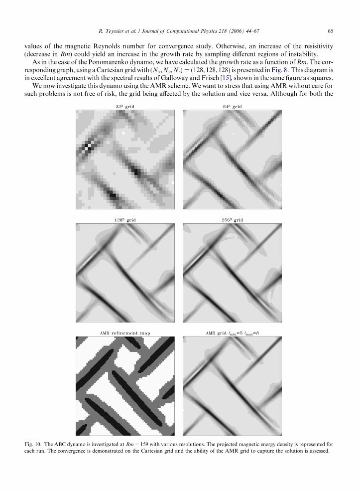
As in the case of the Ponomarenko dynamo, we have calculated the growth rate as a function of Rm. The cor-responding graph, using a Cartesian grid with (Nx,Ny,Nz) = (128, 128,128) is presented in Fig. 8 . This diagram isin excellent agreement with the spectral results of Galloway and Frisch [15], shown in the same figure as squares.

We now investigate this dynamo using the AMR scheme. We want to stress that using AMR without care forsuch problems is not free of risk, the grid being affected by the solution and vice versa. Although for both the

Fig. 10. The ABC dynamo is investigated at Rm = 159 with various resolutions. The projected magnetic energy density is represented foreach run. The convergence is demonstrated on the Cartesian grid and the ability of the AMR grid to capture the solution is assessed.


advection and Ponomarenko tests, the solution has been well captured using straightforward refinement crite-ria, the situation is more subtle for the ABC flow, for which the field generation is not localized. If the strategy isnot adequate, some regions of the flow might not be refined as they should be, and thus be subject to a largeamount of numerical diffusivity. The choice of the optimal refinement strategy for the ABC flow is beyondthe scope of the present study. It could for example be based on various flow properties, such as Liapunov expo-nents, stagnation points, etc., or on various field properties, such as gradients, truncation errors, etc.

As a first step, we have used here a criterion based on the magnetic energy density which allows the grid tobe easily densified near the cigar-like structures: when the local magnetic energy density on level 5, 6, 7, . . . is,respectively, greater than 4, 16, 64. . . times the mean energy density, new refinements are triggered. This strat-egy is best applied at large Rm for which the magnetic structures are well localized. We focus here onRm = 159( = 1000/2p).

The AMR simulation yields a growth rate of 0.052 after 77 h of wall-time computing using eight processors.It is evolved until t = 80. At that time, the grid is composed of 455,659 cells. The structure of the eigenmodeand the topology of the grid are illustrated in Fig. 9. For comparison, the Cartesian grid simulation with 2563

cells yields a growth rate of 0.055 but requires 138 h to evolve the solution only up to t = 46 and using 64 pro-cessors! The AMR simulation has therefore allowed a gain in memory of a factor of 37, and a speed-up of 25in time. All our computations are compared in Fig. 10. The first four panels show the projected magneticenergy obtained varying the resolution from 323 to 2563. Computations performed with 1283 and 2563 cellsreveal very little differences and clearly indicate convergence. The two bottom snapshots illustrate the structureof the grid in the AMR simulations (left panel) and the projected magnetic energy (right panel). There is agood agreement between the AMR simulation and the run performed on the 2563 grid (about 10%).

5. Conclusions and perspectives

We have shown that the constrained transport approach for preserving the solenoidal character of the mag-netic field could be combined with a Godunov method, provided a two-dimensional Riemann solver can beused. We have further shown how this could be combined with a MUSCL high order scheme. We consideredthree schemes for the predictive step, each with its own merits. For a uniform velocity field, these CT schemesare strictly equivalent to well known finite-volume schemes on the staggered grid. This important result pro-vides additional support to the advection properties of the CT framework.

We have implemented this strategy on a kinematic dynamo problem, for which only the induction equationneeds to be considered. We have shown that the Godunov framework allows an efficient AMR treatment offast dynamos, by ensuring the numerical stability of the scheme in regions solved with a coarse grid (for whichthe effects of the physical diffusion are vanishing).

The approach introduced here clearly needs to be adapted to the full set of MHD equations, for which solv-ing the Riemann problem is no longer a trivial task. This important step raises several additional difficultiesand is the object of a forthcoming paper [14].

Acknowledgments

We thank Stephane Colombi for many useful discussions and for help with the OpenMP implementation.We are most grateful to Patrick Hennebelle for suggesting the use of the C-MUSCL scheme. Computationswere performed on supercomputers at CCRT (CEA Bruyeres-le-Chatel), DMPN (IPGP), and QMUL-HPCF(SRIF).

References

[1] V. Archontis, S.B.F. Dorch, A. Nordlund, Numerical simulations of kinematic dynamo action, Astron. Astrophys. 397 (2003) 393–399.

[2] D.S. Balsara, Divergence-free adaptive mesh refinement for magnetohydrodynamics, J. Comput. Phys. 174 (2) (2001) 614–648.[3] D.S. Balsara, D.S. Spicer, A staggered mesh algorithm using high order Godunov fluxes to ensure solenodial magnetic fields in

magnetohydrodynamic simulations, J. Comput. Phys. 149 (2) (1999) 270–292.[4] M.J. Berger, P. Colella, Local adaptive mesh refinement for shock hydrodynamics, J. Comput. Phys. 82 (1989) 64–84.


[5] M.J. Berger, J. Oliger, Adaptive mesh refinement for hyperbolic partial differential equations, J. Comput. Phys. 53 (1984) 484–512.[6] F. Bouchut, Non-linear Stability of Finite Volume Methods for Hyperbolic Conservation Laws. Frontiers in Mathematics,

Birkhauser, Basel, 2005.[7] J.U. Brackbill, D.C. Barnes, The effect of nonzero product of magnetic gradient and B on the numerical solution of the

magnetohydrodynamic equations, J. Comput. Phys. 35 (May) (1980) 426–430.[8] S. Childress, A.D. Gilbert, Stretch, Twist, Fold. The Fast Dynamo, XILecture Notes in Physics, vol. 37, Springer, Berlin, 1995,

406pp.[9] U.R. Christensen, J. Aubert, P. Cardin, E. Dormy, S. Gibbons, G.A. Glatzmaier, E. Grote, Y. Honkura, C. Jones, M. Kono, M.

Matsushima, A. Sakuraba, F. Takahashi, A. Tilgner, J. Wicht, K. Zhang, A numerical dynamo benchmark, Phys. Earth PlanetaryInteriors 128 (2001) 25–34.

[10] P. Colella, Multidimensional upwind methods for hyperbolic conservation laws, J. Comput. Phys. 87 (1) (1990) 171–200.[11] R.K. Crockett, P. Colella, R.T. Fisher, R.I. Klein, C.F. McKee, An unsplit, cell-centered Godunov method for ideal mhd, J. Comput.

Phys. 203 (2005) 422–448.[12] A. Dedner, F. Kemm, D. Kroner, C.D. Munz, T. Schnitzer, M. Wesenberg, Hyperbolic divergence cleaning for the MHD equations,

J. Comput. Phys. 175 (2002) 645–673.[13] C.R. Evans, J.F. Hawley, Simulation of magnetohydrodynamic flows – A constrained transport method, Astrophys. J. 332 (1988)

659–677.[14] S. Fromang, P. Hennebelle, R. Teyssier, A high order AMR Godunov code for astrophysical MHD, Astron. Astrophys. (in

preparation).[15] D.J. Galloway, U. Frisch, Dynamo action in a family of flows with chaotic streamlines, Geophys. Astrophys. Fluid Dyn. 36 (1986)

53–83.[16] T.A. Gardiner, J.M. Stone, An unsplit Godunov method for ideal MHD via constrained transport, J. Comput. Phys. 205 (2005) 509–

539.[17] A. Gilbert, Fast dynamo action in the Ponomarenko dynamo, Geophys. Astrophys. Fluid Dyn. 44 (1988) 241–258.[18] H. Harder, U. Hansen, A finite-volume solution method for thermal convection and dynamo problems in spherical shells, Geophys. J.

Int. 161 (2005) 522–532.[19] A.M. Khokhlov, Fully threaded tree algorithms for adaptive refinement fluid dynamics simulations, J. Comput. Phys. 143 (2) (1998)

519–543.[20] J. Kleimann, A. Kopp, H. Fichtner, R. Grauer, K. Germaschewski, Three-dimensional MHD high-resolution computations with

CWENO employing adaptive mesh refinement, Comput. Phys. Commun. 158 (2004) 47–56.[21] A.V. Kravtsov, A.A. Klypin, A.M. Khokhlov, Adaptive refinement tree: a new high-resolution N-body code for cosmological

simulations, Astrophys. J. Suppl. Ser. 111 (1997) 73.[22] S. Li, H. Li, A novel approach of divergence-free reconstruction for adaptive mesh refinement, J. Comput. Phys. 199 (1) (2004) 1–15.[23] P. Londrillo, L. Del Zanna, High-order upwind schemes for multidimensional magnetohydrodynamics, Astrophys. J. 530 (2000) 508–

524.[24] P. Londrillo, L. Del Zanna, On the divergence-free condition in Godunov-type schemes for ideal magnetohydrodynamics: the upwind

constrained transport method, J. Comput. Phys. 195 (2004) 17–48.[25] H. Matsui, H. Okuda, MHD dynamo simulation using the GeoFEM platform – verification by the dynamo benchmark test, Int. J.

Comput. Fluid Dyn. 19 (2005) 15–22.[26] F. Plunian, P. Masse, Couplage magnetohydraulique: modelisation de la dynamo cinematique, in: Meunier G. Hermes (Ed.),

Electromagnetisme et elements finis, vol. 3, 2002, pp. 215–247.[27] Y. Ponomarenko, On the theory of hydromagnetic dynamos (English translation), J. Appl. Mech. Tech. Phys. 14 (1973) 775–778.[28] S. Popinet, Gerris: a tree-based adaptive solver for the incompressible Euler equations in complex geometries, J. Comput. Phys. 190

(2) (2003) 572–600.[29] K.G. Powell, P.L. Roe, T.J. Linde, T.I. Gombosi, D.L. De Zeeuw, A solution-adaptive upwind scheme for ideal magnetohydro-

dynamics, J. Comput. Phys. 154 (1999) 284–309.[30] D. Ryu, F. Miniati, T.W. Jones, A. Frank, A divergence-free upwind code for multidimensional magnetohydrodynamic flows,

Astrophys. J. 509 (1998) 244–255.[31] R. Samtaney, S.C. Jardin, P. Colella, D.F. Martin, 3D adaptive mesh refinement simulations of pellet injection in tokamaks, Comput.

Phys. Commun. 164 (2004) 220–228.[32] R. Teyssier, Cosmological hydrodynamics with adaptive mesh refinement. A new high resolution code called RAMSES, Astron.

Astrophys. 385 (2002) 337–364.[33] E. Toro, Riemann Solvers and Numerical Methods for Fluid Dynamics, Springer, Berlin, 1999.[34] G. Toth, The $ Æ B = 0 constraint in shock-capturing magnetohydrodynamics codes, J. Comput. Phys. 161 (2) (2000) 605–652.[35] G. Toth, P.L. Roe, Divergence- and curl-preserving prolongation and restriction formulas, J. Comput. Phys. 180 (2) (2002) 736–750.[36] B. van Leer, Towards the ultimate conservative difference scheme: IV. A new approach to numerical convection, J. Comput. Phys. 23

(1977) 276–299.[37] K. Yee, Numerical solution of initial boundary value problems involving Maxwell equations in isotropic media, IEEE Trans. Antenna

Propag. 302 (1966).[38] U. Ziegler, A three-dimensional Cartesian adaptive mesh code for compressible magnetohydrodynamics, Comput. Phys. Commun.

116 (1999) 65–77.

Kinematic dynamos using constrained transport with high ...dormy/Publications/TFD06.pdf ·...

Documents

Transcript of Kinematic dynamos using constrained transport with high ...dormy/Publications/TFD06.pdf ·...