Machine Learning, 55, 53–69, 2004c© 2004 Kluwer Academic Publishers. Manufactured in The Netherlands.

Khiops: A Statistical Discretization Methodof Continuous Attributes

MARC BOULLE marc.boulle@francetelecom.comFrance Telecom R&D, 2, Avenue Pierre Marzin, 22300 Lannion, France

Editor: Peter Flach

Abstract. In supervised machine learning, some algorithms are restricted to discrete data and have to discretizecontinuous attributes. Many discretization methods, based on statistical criteria, information content, or otherspecialized criteria, have been studied in the past. In this paper, we propose the discretization method Khiops,1 basedon the chi-square statistic. In contrast with related methods ChiMerge and ChiSplit, this method optimizes the chi-square criterion in a global manner on the whole discretization domain and does not require any stopping criterion.A theoretical study followed by experiments demonstrates the robustness and the good predictive performance ofthe method.

Keywords: data mining, machine learning, discretization, data analysis

1. Introduction

Discretization of continuous attributes is a problem that has been studied extensivelyin the past (Catlett, 1991; Holte, 1993; Dougherty, Kohavi, & Sahami, 1995; Zighed &Rakotomalala, 2000). Many induction algorithms rely on discrete attributes, and need todiscretize continuous attributes, i.e. to slice their domain into a finite number of intervals.For example, decision tree algorithms exploit a discretization method to handle continu-ous attributes. C4.5 (Quinlan, 1993) uses the information gain based on Shannon entropy.CART (Breiman, 1984) applies the Gini criterion (a measure of the impurity of the intervals).CHAID (Kass, 1980) relies on a discretization method close to ChiMerge (Kerber, 1991).SIPINA takes advantage of the Fusinter criterion (Zighed, 1998) based on measures of un-certainty that are sensitive to sample size. While most discretization methods are employedas a preprocessing step to an induction algorithm, there are still other approaches, similarto the wrapper approach involved in the feature selection field. For example, Bertelsen andMartinez (1994) and Burdsall and Giraud-Carrier (1997) propose approaches that allow torefine the discretization of the continuous explanatory attributes by taking feedback froman induction algorithm.

Most discretization methods are divided into top-down and bottom-up methods. Top-down methods start from the initial interval and recursively split it into smaller intervals.Bottom-up methods start from the set of single value intervals and iteratively merge neigh-boring intervals. Some of these methods require user parameters to modify the behavior ofthe discretization criterion or to set up a threshold for the stopping rule. In the discretizationproblem, a compromise must be found between information quality (homogeneous intervals

54 M. BOULLE

in regard to the attribute to predict) and statistical quality (sufficient sample size in everyinterval to ensure generalization). The chi-square-based criteria focus on the statistical pointof view whereas the entropy-based criteria focus on the information point of view. Othercriteria (such as Gini or Fusinter criterion) try to find a trade off between information andstatistical properties. The Minimum Description Length (MDL) criterion (Fayyad, 1992)is an original approach that attempts to minimize the total quantity of information bothcontained in the model and in the exceptions to the model.

We present a new discretization method named Khiops. This is a bottom-up method basedon the global optimization of chi-square. The most similar existing methods are the top-down and bottom-up methods using the chi-square criterion in a local manner. The top-downmethod based on chi-square is ChiSplit (Bertier & Bouroche, 1981). It searches for the bestsplit of an interval, by maximizing the chi-square criterion applied to the two sub-intervalsadjacent to the splitting point: the interval is split if both sub-intervals substantially differstatistically. The ChiSplit stopping rule is based on a user-defined chi-square threshold toreject the split if the two sub-intervals are too similar. The bottom-up method based onchi-square is ChiMerge (Kerber, 1991). It searches for the best merge of adjacent intervalsby minimizing the chi-square criterion applied locally to two adjacent intervals: they aremerged if they are statistically similar. The stopping rule is based on a user-defined chi-square threshold to reject the merge if the two adjacent intervals are insufficiently similar.

The Khiops method proposed in this paper starts the discretization from the elementarysingle value intervals. It evaluates all merges between adjacent intervals and selects the bestone according to the chi-square criterion applied to the whole set of intervals. The stoppingrule is based on the confidence level computed with the chi-square statistic. The methodautomatically stops merging intervals as soon as the confidence level, related to the chi-square test of independence between the discretized attribute and the class attribute, doesnot decrease anymore. The Khiops method optimizes a global criterion that evaluates thepartition of the domain into intervals, as opposed to a local criterion applied to two neigh-boring intervals as in ChiSplit or ChiMerge. The absence of user parameters makes themethod very convenient to use and allows to automatically obtain high-quality discretiza-tions. We will demonstrate that in spite of this global approach, the Khiops approach can beimplemented such that its run-time is super-linear in the sample size. This computationalcomplexity is the same as that of the optimized version of the ChiMerge algorithm. We willcompare the Khiops method with other discretization methods by means of experiments onstandard benchmarks.

The remainder of the paper is organized as follows. Section 2 presents the Khiops al-gorithm and its main properties. Section 3 compares the Khiops method with the relatedChiMerge and ChiSplit methods from a theoretical point of view. Section 4 proceeds withan extensive experimental evaluation.

2. The Khiops discretization method

In this section, we first recall the principles of the chi-square test and then present the Khiopsalgorithm. Next, we focus on the computational complexity of the algorithm, and finally,we discuss some practical issues.

KHIOPS: A STATISTICAL DISCRETIZATION METHOD 55

Table 1. Contingency table used to compute the chi-square value.

A B C Totalni j : Observed frequency for i th explanatory valueand j th class value a n11 n12 n13 n1

ni.: Total observed frequency for i th explanatory value b n21 n22 n23 n2

n. j : Total observed frequency for j th class value c n31 n32 n33 n3

N : Total observed frequency d n41 n42 n43 n4

I : Number of explanatory attribute values e n51 n52 n53 n5

J : Number of class values Total n.1 n.2 n.3 N

2.1. The chi-square test: Principles and notations

Let us consider an explanatory attribute (a feature) and a class attribute, and determinewhether they are independent. First, all instances are summarized in a contingency table,where the instances are counted for each value pair of explanatory and class attributes. Thechi-square value is computed from the contingency table.

Let ei j = ni.∗ n. j/N . ei j stands for the expected frequency for cell (i, j) if the explanatoryand class attributes are independent.

The chi-square value is a measure on the whole contingency table of the differencebetween observed frequencies and expected frequencies. It can be interpreted as a distanceto the hypothesis of independence between attributes.

Chi2 =∑

i

∑j

(ni j − ei j )2

ei j

If the hypothesis of independence is true, the chi-square value is distributed as a chi-squarestatistic with (I − 1) ∗ (J − 1) degrees of freedom. This is the basis for a statistical test thatallows rejecting the hypothesis of independence. The confidence level is the probability ofthe hypothesis of independence. For example, in a contingency table of size 5 ∗ 3 (whichcorresponds to a chi-square statistic with 8 degrees of freedom), the confidence level asso-ciated to a chi-square value of 20 is about 1%. This means that when the explanatory andthe class attributes are independent, the probability of observing a chi-square value greaterthan 20 is less than 1%. The higher the chi-square value is, the smaller is the confidencelevel.

2.2. Algorithm

The chi-square value depends both on the local observed frequencies in each individualrow and on the global observed frequencies in the whole contingency table. This is a goodcandidate criterion for a discretization method. The chi-square statistic is parameterized bythe number of explanatory values (related to the degrees of freedom). In order to comparetwo discretizations with different interval numbers, we will use the confidence level insteadof the chi-square value.

The principle of the Khiops algorithm is to minimize the confidence level between thediscretized explanatory attribute and the class attribute by means of the chi-square statistic.

56 M. BOULLE

The chi-square value is not reliable to test the hypothesis of independence if the expectedfrequency in any cell of the contingency table is less than some minimum value. This isequivalent to a minimum frequency constraint for each row of the contingency table, i.e.for each interval of the discretization. The algorithm will cope with this constraint.

The Khiops method is based on a greedy bottom-up algorithm. It starts with initial singlevalue intervals and then searches for the best merge between adjacent intervals. Two differenttypes of merges are encountered. First, merges with at least one interval that does not meetthe constraint and second, merges with both intervals fulfilling the constraint. The bestmerge candidate (with the highest chi-square value) is chosen in priority among the firsttype of merges (in which case the merge is accepted unconditionally), and otherwise, if allminimum frequency constraints are respected, among the second type of merges (in whichcase the merge is accepted under the condition of improvement of the confidence level).The algorithm is reiterated until both all minimum frequency constraints are respected andno further merge can decrease the confidence level.

Algorithm. Khiops

1. Initialization

1.1. Sort the explanatory attribute values1.2. Create an elementary interval for each value

2. Optimization of the discretizationRepeat the following steps:

2.1. Search for the best mergeSearch among the merges with at least one interval that does not meet the frequencyconstraint if anyone exists, among any merge otherwiseMerge that maximizes the chi-square value

2.2. Evaluate the stopping ruleStop if all constraints are respected and if no further merge decreases the confidencelevel

2.3. Merge and continue if the stopping rule is not met

2.3. Minimum frequency per interval

In order to be reliable, the chi-square test requires that every cell of the contingency tablehas an expected value of at least 5. This reliability constraint is equivalent to a minimumfrequency constraint for each interval of the discretization.

The purpose of the Khiops discretization algorithm is to approximate the true classattribute distribution from the observed distribution of the training sample on the basis ofintervals, which result from a supervised merging process. This process can be consideredas an inductive algorithm, therefore subject to overfitting. In order to prevent overfitting, asolution is to increase the minimum frequency per interval constraint. The Khiops algorithmuses a heuristic control of overfitting by constraining the intervals to have a frequencygreater than the square root of the sample size. This value allows both to improve the

KHIOPS: A STATISTICAL DISCRETIZATION METHOD 57

statistical reliability of the observed distribution in each interval and to refine the precisionof the discretization owing to a potentially higher number of intervals when the sample sizeincreases.

To improve the chi-square test reliability and to prevent overfitting, the Khiops algorithmis constrained to employ the maximum of the two preceding values.

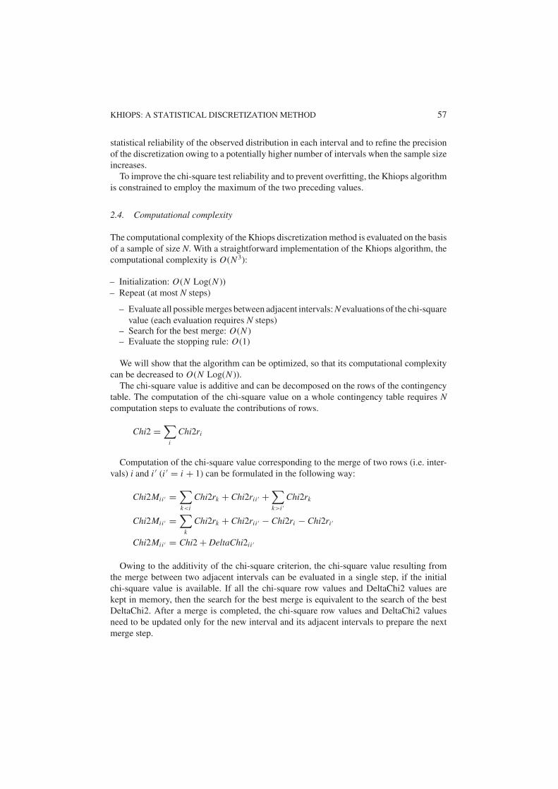
2.4. Computational complexity

The computational complexity of the Khiops discretization method is evaluated on the basisof a sample of size N. With a straightforward implementation of the Khiops algorithm, thecomputational complexity is O(N 3):

– Initialization: O(N Log(N ))– Repeat (at most N steps)

– Evaluate all possible merges between adjacent intervals: N evaluations of the chi-squarevalue (each evaluation requires N steps)

– Search for the best merge: O(N )– Evaluate the stopping rule: O(1)

We will show that the algorithm can be optimized, so that its computational complexitycan be decreased to O(N Log(N )).

The chi-square value is additive and can be decomposed on the rows of the contingencytable. The computation of the chi-square value on a whole contingency table requires Ncomputation steps to evaluate the contributions of rows.

Chi2 =∑

i

Chi2ri

Computation of the chi-square value corresponding to the merge of two rows (i.e. inter-vals) i and i ′ (i ′ = i + 1) can be formulated in the following way:

Chi2Mii ′ =∑k<i

Chi2rk + Chi2rii ′ +∑k>i ′

Chi2rk

Chi2Mii ′ =∑

k

Chi2rk + Chi2rii ′ − Chi2ri − Chi2ri ′

Chi2Mii ′ = Chi2 + DeltaChi2i i ′

Owing to the additivity of the chi-square criterion, the chi-square value resulting fromthe merge between two adjacent intervals can be evaluated in a single step, if the initialchi-square value is available. If all the chi-square row values and DeltaChi2 values arekept in memory, then the search for the best merge is equivalent to the search of the bestDeltaChi2. After a merge is completed, the chi-square row values and DeltaChi2 valuesneed to be updated only for the new interval and its adjacent intervals to prepare the nextmerge step.

58 M. BOULLE

The critical part of the algorithm corresponds to the search for the best merge. This searchneeds N steps. If the list of all possible merges is initially sorted, and if this list remainssorted during the discretization process, the search for the best merge takes one step, at theexpense of the cost needed to keep the list sorted. Balanced binary search trees (such asAVL binary search trees for example) allow to keep a list sorted when elements are insertedor deleted, with a logarithmic computational complexity.

Finally, the computational complexity of the optimized version of Khiops algorithm canbe decreased to O(N Log(N )) if the chi-square row values and the DeltaChi2 values arekept in memory, if the chi-square values are computed in an additive way and if the mergesare stored in a maintained sorted list.

The memory requirement of the algorithm is also O(N Log(N )). Data that need to bekept in memory are the N chi-square row values, the N DeltaChi2 values and the sorted listof merges, which has a memory requirement of O(N Log(N )).

Algorithm. Optimized Khiops

1. Initialization

1.1. Sort the explanatory attribute values: O(N log(N ))1.2. Create an elementary interval for each value: O(N )1.3. Compute the chi-square row values and the initial chi-square value: O(N )1.4. Compute the DeltaChi2 values: O(N )1.5. Sort the possible merges: O(N Log(N ))1.6. Compute the confidence level of this first discretization: O(1)

2. Optimization of the discretizationRepeat the following steps: at most N steps

2.1. Search for the best possible merge: O(1)2.2. Evaluate the stopping rule: O(1)

Stop if all constraints are respected and if no further merge decreases the confidencelevel

2.3. Merge and continue if the stopping rule is not met

2.3.1. Compute the chi-square row value for the new interval: O(1)2.3.2. Compute the DeltaChi2 values for the two intervals adjacent to the new

interval: O(1)2.3.3. Update the sorted list of merges: O(log(N ))

Remove the merge just completedRemove the two merges of the intervals adjacent to the former sub-intervalsof the new intervalAdd the two merges of the intervals adjacent to the new interval

The optimized version of the Khiops algorithm has the same computational complexityas the optimized version of the ChiMerge algorithm. This property allows the method to beeffective on large databases (containing at least 105 instances).

KHIOPS: A STATISTICAL DISCRETIZATION METHOD 59

2.5. Practical issues

There is a potential gap between the principles and the implementation of the algorithm.The principle of the algorithm is to search, among all possible sets of intervals, the set thatminimizes the confidence level of the test of independence between the discretized attributeand the class attribute. This confidence level is evaluated with the chi-square statistic appliedto the corresponding contingency table. To improve the statistical reliability of the algorithm,a minimum frequency related to the sample size is used to constrain the search of the bestset of intervals. Based on these principles, the Khiops method seems robust. However,problems so far overlooked are now discussed.

The value used for the minimum frequency constraint is a heuristic choice and has nostrong foundation. To be more consistent, this value should result from some statisticalestimation that precisely takes into account the distribution of the class values and controlsthe probability of overfitting. Such an estimation, involving complex calculation, is beyondthe scope of this paper.

The search algorithm is a greedy algorithm that tries to follow the minimum frequencyconstraint in a very simple and flexible way. This heuristic leads to super-linear computationtime, which is mandatory as soon as large databases are processed. However, the searchalgorithm can be trapped in a local optimum and has no guarantee to find the best set ofintervals. It is still not realistic to find the best discretization when computation time is anissue.

The algorithm needs a good evaluation of the chi-square statistic for very large chi-squarevalues and degrees of freedom. Such a good evaluation is not presently available in standardnumerical libraries. Furthermore, the limits of numerical precision of computer are rapidlyovertaken when the confidence level gets too close to zero.

The practical limits of the Khiops discretization method are principally related to itsimplementation. The most critical issue is the evaluation of the chi-square statistic in a verylarge numerical domain. This problem has been studied and solved in Boulle (2001). Thesolution relies on a good approximation of the logarithm of the confidence level, and forbetter accuracy, on a precise evaluation of the variation threshold of the chi-square valuethat controls the stopping rule used in the Khiops algorithm.

We illustrate that in extensive experiments, in spite of the raw value used for the minimumfrequency constraint and of the greedy search algorithm, the Khiops algorithm allowsobtaining high quality discretizations together with fast computation time.

3. Theoretical comparison with the chi-square-based discretization methods

In this section, we compare the Khiops method with the related ChiMerge and ChiSplitmethods, and show that the Khiops method solves several weaknesses of the other methods.

3.1. Properties of merges in the Khiops method

In this section, we demonstrate that when two rows of a contingency table are merged, thewhole chi-square value can only decrease. However, after a merge, the chi-square statistic

60 M. BOULLE

is based on fewer degrees of freedom. If the whole chi-square value decreases very little(or does not decrease at all), the related confidence level also decreases; otherwise theconfidence level increases.

Theorem. When two rows of a contingency table are merged, the chi-square value of thecontingency table decreases.

Proof: Let p1, p2, . . . , pJ be the probabilities of the class values in the complete contin-gency table.∑

j

p j = 1.

Let a1, a2, . . . , aJ and b1, b2, . . . , bJ be the probabilities of the class values in twoadjacent rows of the contingency table with row frequencies n and n′.∑

j

a j = 1.∑

j

b j = 1.

The observed and expected frequencies are a j n and p j n in the first row, b j n′ and p j n′

in the second row. The chi-square row values Chi2r and Chi2r′ are

Chi2r = n

( ∑j

a2j

/p j − 1

)and Chi2r ′ = n′

( ∑j

b2j

/p j − 1

)

Let us consider the merge of the two rows. The observed and expected frequencies in themerged row are a j n + b j n′ and p j (n + n′).

The chi-square merged row value Chi2l′′ is

Chi2r ′′ = (n + n′)

( ∑j

((a j n + b j n′)/(n + n′))2

p j− 1

)(1)

The merge between the two rows causes an update of the whole chi-square valueDeltaChi2 = Chi2r ′′ − Chi2r − Chi2r ′.

DeltaChi2 =∑

j

(n + n′)((a j n + b j n′)/(n + n′))2 − na2j − n′b2

j

p j(2)

DeltaChi2 = − nn′

n + n′∑

j

(a j − b j )2

p j(3)

This last formula shows that the chi-square value of the contingency table decreases afterthe merge.

KHIOPS: A STATISTICAL DISCRETIZATION METHOD 61

3.2. Comparison with the ChiMerge method

For the ChiMerge discretization method, let us consider the local contingency table restrictedto the two rows. Let q1, q2, . . . , qJ . be the probabilities of the class values in this localcontingency table.

∑j

q j = 1. q j = (a j n + b j n′)/(n + n′).

In order to evaluate the merge of the two rows, let us calculate the local chi-square value.

LocalChi2 = n

( ∑j

a2j

/q j − 1

)+ n′

( ∑j

b2j

/q j − 1

)(4)

LocalChi2 = nn′

n + n′∑

j

(a j − b j )2

q j(5)

The stopping rules used in the Khiops and ChiMerge methods are based on similarmathematical formulas, but the two discretization methods lead to a large difference ininterpretation of the formulas. The probabilities of the class values are global to the wholecontingency table for the Khiops method (p j probabilities) whereas they are local to thetwo rows for the ChiMerge method (q j probabilities).

For the Khiops method, the stopping rule is:

Prob(Chi2 + DeltaChi2, (I − 2) ∗ (J − 1)) < Prob(Chi2, (I − 1) ∗ (J − 1)) (6)

For the ChiMerge method (with a user parameter ProbThreshold), the stopping rule is:

Prob(LocalChi2, J − 1) > ProbThreshold (7)

This demonstrates an important difference between the two methods. The ChiMergemethod acts locally, whereas the Khiops method takes into account the whole distributionof the class values, the whole number of intervals and the global chi-square value.

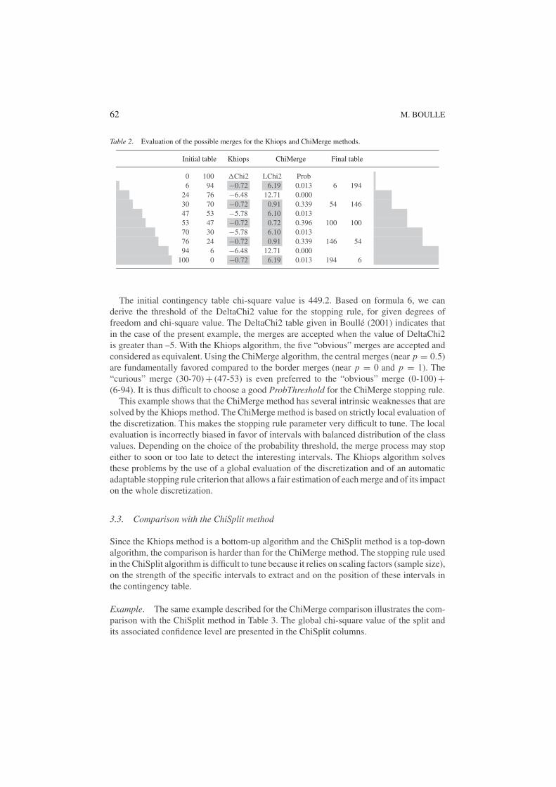
Example. We present an example in Table 2, which illustrates the difficulty in choosing theProbThreshold user parameter in the ChiMerge algorithm. In Table 2, the initial contingencytable on the left summarizes a sample with 1000 instances and two equidistributed classvalues. The rows (i.e intervals) of the initial table have an increasing proportion of the firstclass value, and the successive pairs of intervals have similar proportions of class values.The “natural” discretization of this table ends with the final contingency table shown onthe right. The DeltaChi2 and LocalChi2 (with related confidence level) evaluations of thepossible merges in the Khiops and ChiMerge methods are presented in the middle columns.The grayed values correspond to the preferred merges for each method.

62 M. BOULLE

Table 2. Evaluation of the possible merges for the Khiops and ChiMerge methods.

Initial table Khiops ChiMerge Final table

0 100 �Chi2 LChi2 Prob6 94 −0.72 6.19 0.013 6 194

24 76 −6.48 12.71 0.00030 70 −0.72 0.91 0.339 54 14647 53 −5.78 6.10 0.01353 47 −0.72 0.72 0.396 100 10070 30 −5.78 6.10 0.01376 24 −0.72 0.91 0.339 146 5494 6 −6.48 12.71 0.000

100 0 −0.72 6.19 0.013 194 6

The initial contingency table chi-square value is 449.2. Based on formula 6, we canderive the threshold of the DeltaChi2 value for the stopping rule, for given degrees offreedom and chi-square value. The DeltaChi2 table given in Boulle (2001) indicates thatin the case of the present example, the merges are accepted when the value of DeltaChi2is greater than –5. With the Khiops algorithm, the five “obvious” merges are accepted andconsidered as equivalent. Using the ChiMerge algorithm, the central merges (near p = 0.5)are fundamentally favored compared to the border merges (near p = 0 and p = 1). The“curious” merge (30-70) + (47-53) is even preferred to the “obvious” merge (0-100) +(6-94). It is thus difficult to choose a good ProbThreshold for the ChiMerge stopping rule.

This example shows that the ChiMerge method has several intrinsic weaknesses that aresolved by the Khiops method. The ChiMerge method is based on strictly local evaluation ofthe discretization. This makes the stopping rule parameter very difficult to tune. The localevaluation is incorrectly biased in favor of intervals with balanced distribution of the classvalues. Depending on the choice of the probability threshold, the merge process may stopeither to soon or too late to detect the interesting intervals. The Khiops algorithm solvesthese problems by the use of a global evaluation of the discretization and of an automaticadaptable stopping rule criterion that allows a fair estimation of each merge and of its impacton the whole discretization.

3.3. Comparison with the ChiSplit method

Since the Khiops method is a bottom-up algorithm and the ChiSplit method is a top-downalgorithm, the comparison is harder than for the ChiMerge method. The stopping rule usedin the ChiSplit algorithm is difficult to tune because it relies on scaling factors (sample size),on the strength of the specific intervals to extract and on the position of these intervals inthe contingency table.

Example. The same example described for the ChiMerge comparison illustrates the com-parison with the ChiSplit method in Table 3. The global chi-square value of the split andits associated confidence level are presented in the ChiSplit columns.

KHIOPS: A STATISTICAL DISCRETIZATION METHOD 63

Table 3. Evaluation of the possible merges for the Khiops and ChiSplit methods.

Initial table Khiops ChiSplit Final table

0 100 �Chi2 Chi2S Prob6 94 −0.72 111.11 5.59E-26 6 194

24 76 −6.48 220.90 5.76E-5030 70 −0.72 274.29 1.32E-61 54 14647 53 −5.78 326.67 5.11E-7353 47 −0.72 327.18 3.95E-73 100 10070 30 −5.78 326.67 5.11E-7376 24 −0.72 274.29 1.32E-61 146 5494 6 −6.48 220.90 5.76E-50

100 0 −0.72 111.11 5.59E-26 194 6

According to Table 3, the confidence level used for the ChiSplit stopping rule shouldbe set between 10−25 and 10−75. For larger sample sizes (more than 10000 instances),this confidence level would be above the limit of numerical precision of computers (about10−300), and thus the choice of a confidence level becomes impossible. Furthermore, thebest split found by the ChiSplit method lies exactly in the middle of the contingency table.This split produces two intervals (107-393) and (393-107) and is actually an excellent splitof the table into two intervals. However, this split has definitely separated rows (47-53) and(53-47) that should be “intuitively” merged together.

Problem of nested interesting intervals. The ChiSplit top-down approach has a more seri-ous drawback. It cannot discover interesting intervals nested between regular intervals sincethis requires two successive splits with the first one not very significant. We demonstratethis rigorously with the use of artificial data, consisting of two equidistributed intervals I1and I3 with global frequency 1000, surrounding one interesting interval I2 with frequency50:

– I1: (250-250)– I2: (50-0)– I3: (250-250)

With the ChiSplit method, the two possible splits have a chi-square value of 2.17 related toa confidence level of 0.14. With a ChiSplit stopping criterion threshold set to 0.05, the twosplits are rejected and thus the interesting interval cannot be found. With the Khiops method,the initial contingency table has a chi-square value of 47.7 related to a confidence level of4.3 10−11. The two possible merges are rejected because they increase the confidence level,and the interesting interval is therefore correctly identified.

In figure 1, we study the impact of the position of the interesting interval I2 (i.e. thenumber of instances in I1) on the behavior of the methods. Table A stands for the bipartition{I1 ∪ I2, I3} of the initial intervals. Table A can be seen both as a split after the interestinginterval for the ChiSplit method and as a merge of the two first intervals for the Khiops

64 M. BOULLE

Initial table

I1 I2 I3

Table A

I1 I2 I3

Table B

I1 I2 I3

Confidence Level

1.0E-11

1.0E-10

1.0E-09

1.0E-08

1.0E-07

1.0E-06

1.0E-05

1.0E-04

1.0E-03

1.0E-02

1.0E-01

1.0E+00

0 100 200 300 400 500 600 700 800 900 1000

Position of interval I2

Initial table

Table A

Table B

5% threshold

Figure 1. Confidence level related to the chi-square test for the initial table {I1, I2, I3}, the Table A {I1 ∪ I2, I3}and the Table B {I1, I2 ∪ I3}.

method. Table B is defined in the same way with a partition {I1, I2 ∪ I3} of the initialintervals. Figure 1 shows that with the Khiops method, the confidence level of the initialtable is always below that of the two tables resulting from the merges. The merges are thusrejected and the Khiops method always correctly detects the interesting interval. With theChiSplit method, the best split among Table A and Table B corresponds to the table with thelowest confidence level. The ChiSplit method therefore detects the interesting interval onlyif it is situated at the beginning of the contingency table (before position 350 and the splitleads to Table A) or at the end (after position 650 and the split leads to Table B). However,in about one third of the positions, when the interesting interval is around the middle of thecontingency table, both splits are rejected because their confidence level are above the 5%threshold stopping criterion of the algorithm.

The principle used in the ChiSplit method that combines a top-down approach and agreedy algorithm exhibits thus several weaknesses that may prevent the discovery of localpatterns in discretized attributes.

4. Experiments

In our experimental study, we compare the Khiops method with other supervised andunsupervised discretization algorithms considered as a preprocessing step of the NaiveBayes classifier. The Naive Bayes classifier (Langley, Iba, & Thompson, 1992) assigns themost probable class value given the explanatory attribute values, assuming independencebetween the attributes for each class value. After the discretization preprocessing step, theprobabilities of continuous attributes are estimated using counts in each interval.

We gathered 15 datasets from U.C. Irvine repository (Blake, 1998), each dataset has atleast one continuous attribute and at least a few tens of instances for each class value inorder to perform reliable tenfold cross-validations. Table 4 describes the datasets; the lastcolumn corresponds to the relative frequency of the majority class.

KHIOPS: A STATISTICAL DISCRETIZATION METHOD 65

Table 4. Datasets.

Continuous NominalDataset attributes attributes Size Class values Majority class

Adult 7 8 48842 2 76.07

Australian 6 8 690 2 55.51

Breast 10 0 699 2 65.52

Crx 6 9 690 2 55.51

German 24 0 1000 2 70.00

Heart 10 3 270 2 55.56

Hepatitis 6 13 155 2 79.35

Hypothyroid 7 18 3163 2 95.23

Ionosphere 34 0 351 2 64.10

Iris 4 0 150 3 33.33

Pima 8 0 768 2 65.10

SickEuthyroid 7 18 3163 2 90.74

Vehicle 18 0 846 4 25.77

Waveform 21 0 5000 3 33.92

Wine 13 0 178 3 39.89

The discretization methods studied in the comparison are:

– Khiops: the method described in this paper– MDLPC: Minimum Description Length Principal Cut (Fayyad, 1992)– ChiMerge: bottom-up method based on chi-square (Kerber, 1991)– ChiSplit: top-down method based on chi-square (Bertier & Bouroche, 1981)– Equal Width– Equal Frequency

The Khiops and MDLPC methods have an automatic stopping rule and do not requireany parameter setting. For the ChiMerge and ChiSplit methods, the significance level isset to 0.95 for chi-square threshold. For the Equal Width and Equal Frequency unsuper-vised discretization methods, the number of intervals is set to 10. We have re-implementedthese alternative discretization approaches in order to eliminate any variance resulting fromdifferent cross-validation splits.

As the purpose of our experimental study is to compare the discretization methods, wechose to ignore nominal attributes to build the Naive Bayes classifiers. We ran a stratifiedtenfold cross-validation and report the mean and the standard deviation of the accuracies.In order to determine whether accuracies are significantly different between the Khiopsmethod and the alternative methods, the t-statistic of the difference of the accuracies iscomputed. Under the null hypothesis, this value has a Student’s distribution with 9 degreesof freedom. A two-tailed test is appropriate because we do not know in advance whether

66 M. BOULLE

Table 5. Accuracies of the Naive Bayes classifier with different discretization methods.

Dataset Khiops MDLPC ChiMerge ChiSplit Eq. width Eq. freq.

Adult 83.1 ± 0.5 84.4 ± 0.5− 77.8 ± 0.7+ 84.3 ± 0.5− 81.2 ± 0.4+ 81.1 ± 0.6+Australian 78.1 ± 3.9 77.4 ± 3.6 75.1 ± 4.6 78.1 ± 3.5 71.0 ± 5.3+ 80.4 ± 2.4−Breast 97.3 ± 1.2 97.1 ± 1.1 90.1 ± 3.5+ 97.0 ± 1.7 96.6 ± 1.7+ 97.4 ± 1.4

Crx 77.2 ± 4.9 76.5 ± 5.8 71.4 ± 5.9+ 78.0 ± 7.0 70.3 ± 3.6+ 79.7 ± 6.1−German 75.5 ± 3.4 72.5 ± 1.8+ 74.3 ± 3.6 75.6 ± 4.2 75.5 ± 3.6 75.5 ± 3.9

Heart 78.1 ± 7.5 80.7 ± 8.6 72.2 ± 6.3+ 78.9 ± 8.8 81.1 ± 6.5− 80.7 ± 6.6−Hepatitis 78.8 ± 12. 76.8 ± 13. 81.5 ± 11. 78.9 ± 9.5 82.6 ± 8.5 78.8 ± 11.

Hypothyroid 98.0 ± 1.1 98.7 ± 0.6− 98.2 ± 0.6 98.5 ± 1.0 97.4 ± 0.6 97.6 ± 0.9+Ionosphere 89.7 ± 3.2 90.9 ± 4.4 86.1 ± 5.2 86.3 ± 4.0 89.5 ± 4.4 91.2 ± 3.9

Iris 92.0 ± 2.7 92.7 ± 2.0 94.7 ± 2.7− 94.0 ± 3.6 95.3 ± 4.3 94.7 ± 5.0

Pima 75.1 ± 4.4 76.2 ± 2.1 72.0 ± 2.7 75.0 ± 3.0 74.7 ± 3.1 74.0 ± 3.5

SickEuthyroid 96.3 ± 1.0 95.9 ± 1.1 96.3 ± 1.3 95.8 ± 1.0 92.9 ± 1.8+ 93.2 ± 1.1+Vehicle 61.5 ± 2.9 60.2 ± 2.3 64.5 ± 3.8− 63.1 ± 4.1 63.6 ± 3.3 61.4 ± 3.3

Waveform 81.0 ± 1.0 80.8 ± 0.8 75.9 ± 1.6g+ 80.0 ± 1.8+ 80.8 ± 1.2 80.7 ± 1.2

Wine 96.7 ± 2.7 96.7 ± 3.7 96.6 ± 4.5 95.0 ± 3.9 95.5 ± 6.5 96.6 ± 3.7

Mean 83.9 83.8 81.8 83.9 83.2 84.2+ number 1 5 1 5 3

− number 2 2 1 1 3

the mean of the Khiops accuracies is likely to be greater than that of the alternative methodor vice versa. The confidence level is set to 5%.

Table 5 shows the mean and the standard deviation of the accuracies of the Naive Bayesinduction algorithm. The significant wins for the Khiops method are indicated with +, andthe significant losses with −. The Khiops, MDLPC, ChiSplit and EqualFrequency methodshave similar results, and perform better than the ChiMerge and EqualWidth methods. Theseresults allow to distinguish two groups of methods, but are not conclusive enough to furtherrank the methods. The case of the EqualFrequency method (3 wins and 3 losses for theKhiops method) shows that there is a need for more experiments.

In order to analyze the performance of the discretization algorithms more fully, we pro-ceed with the same experiment for each individual continuous attribute in every dataset.These additional experiments are equivalent to 181 experiments with single-attributedatasets. Each discretization method can be evaluated as an elementary attribute classi-fier that predicts the more frequent class value in each learned interval. The results aresummarized in Table 6, which reports for each dataset the mean of the dataset attribute ac-curacies and the number of significant wins and losses of the elementary attribute classifierswhen compared with the Khiops method.

This experiment is more informative than the previous one. It allows a better comparisonbetween the discretization methods, eliminating the bias of the choice of a specific induction

KHIOPS: A STATISTICAL DISCRETIZATION METHOD 67

Table 6. Means of accuracies, number of significant wins and losses per dataset, for the elementary attributeclassifiers.

MDLPC ChiMerge ChiSplit Eq. width Eq. freq.Dataset Khiops + − + − + − + − + −

Adult 77.2 77.3 2 75.7 2 2 77.3 1 2 76.8 2 76.6 2

Australian 64.5 65.0 1 64.7 65.1 1 61.4 3 1 65.7

Breast 86.0 86.1 1 1 85.6 85.9 86.0 85.7 1

Crx 64.5 65.2 63.8 1 65.3 61.1 3 65.6

German 70.0 70.0 70.0 70.1 70.1 1 70.0

Heart 63.8 64.0 64.0 63.8 63.9 64.5

Hepatitis 79.4 79.3 77.8 3 79.3 79.8 79.9

Hypothyroid 96.0 96.1 96.0 3 96.1 1 95.4 3 95.2 3

Ionosphere 78.7 77.6 6 5 75.7 14 79.5 7 73.9 14 1 75.0 17

Iris 77.7 75.5 1 77.0 78.8 76.5 1 76.3

Pima 66.8 66.1 2 65.6 2 66.5 66.8 66.3 1

SickEuthyroid 91.4 91.3 91.3 1 91.3 90.7 2 91.0 1

Vehicle 40.9 40.5 3 2 41.4 1 4 42.1 4 40.8 1 1 40.3 2

Waveform 49.1 49.37 48.7 5 49.1 1 1 49.2 3 1 49.5 1 3

Wine 62.0 60.1 2 59.6 2 60.4 1 61.4 4 1 60.8 1

68.4 68.0 15 11 67.4 34 6 68.6 4 15 67.2 36 6 67.6 28 4

algorithm. The results show that supervised methods (except ChiMerge) perform clearlybetter than unsupervised methods. The ChiMerge method is slightly better than the Equal-Width method, but not as good as the EqualFrequency method. The Khiops method andthe MDLPC method are clearly better than the EqualFrequency, ChiMerge and EqualWidthmethods, with a slight advantage in favor of the Khiops method over the MDPLC method.The ChiSplit method obtains the best results of the experiments. A close look at Table 6indicates a special behaviour of the ionosphere dataset, where the ChiSplit method largelydominates the other methods with 7 wins in the comparison with the Khiops method. Aninspection of the discretizations performed by the ChiSplit algorithm reveals intervals withvery small frequencies, that cannot be found by the Khiops algorithm because of its strictconstraint of minimum frequency per interval.

Although both the Khiops method and the MDLPC method yield comparable results onaverage, they often differ on individual cases. For 181 discretized attributes, there are 15wins for the Khiops method and 11 for the MDPLC method. It can be noticed that thesetwo methods are based on very different approaches. The Khiops method is a bottom-upalgorithm with a global criterion based on the chi-square statistic, whereas the MDLPCmethod is a top-down algorithm with a local criterion based on Shannon entropy.

Despite some theoretical weaknesses, the ChiSplit method obtains better results than theKhiops method. The analysis of partitions of intervals built by the Khiops method revealssome limitation related to the minimum frequency constraint. While this constraint clearlyenhances the reliability of the Khiops method, it prevents it from discovering finely-grained

68 M. BOULLE

patterns in numerical domains. In our future work, we plan to investigate on this minimumfrequency constraint in order to improve the performance of the Khiops method.

The second set of experiments based on single attributes brings useful additional informa-tion to the first set of experiments based on the Naive Bayes classifier. All these results arebased on 15 UCI datasets and 181 continuous attributes, and should be interpreted carefully.However, the main trends expressed by the results allow to rank the tested discretizationmethods in the following way:

1. ChiSplit2. Khiops, MDLPC3. EqualFrequency4. ChiMerge, EqualWidth

The ChiSplit method is the best of the tested methods, while the Khiops method is atleast as good as the MDPLC method.

5. Conclusion

The principle of the Khiops discretization method is to minimize the confidence levelrelated to the test of independence between the discretized explanatory attribute and theclass attribute. This optimization is based on the chi-square criterion applied to the wholeset of intervals of the discretization. This global evaluation carries some intrinsic benefitscompared with the connected ChiMerge and ChiSplit methods. The Khiops automaticstopping rule brings both ease of use and high quality discretizations. Its computationalcomplexity is the same as for the fastest other discretization methods.

Extensive evaluations indicate notable accuracy results for the Khiops method. For furthercomparisons, we plan in future works to study other aspects of evaluation such as therobustness or the size of discretizations.

Acknowledgments

I am grateful to Fabrice Clerot and Jean-Emmanuel Viallet for many insightful discussionsand careful proof reading of the manuscript. I also wish to thank the editor Prof. Peter Flachand the three anonymous reviewers for their beneficial comments.

Note

1. French patent No. 01 07006.

References

Bertelsen, R., & Martinez, T. R. (1994). Extending ID3 through discretization of continuous inputs. In Proceedingsof the 7th Florida Artificial Intelligence Research Symposium (pp. 122–125). Florida AI Research Society.

Bertier, P., & Bouroche, J. M. (1981). Analyse des donnees multidimensionnelles. Presses Universitaires deFrance.

KHIOPS: A STATISTICAL DISCRETIZATION METHOD 69

Blake, C. L., & Merz, C. J. (1998). UCI Repository of machine learning databases [http://www.ics.uci.edu/∼mlearn/MLRepository.html]. Irvine, CA: University of California, Department of Information and ComputerScience.

Boulle, M. (2001). Khiops: Discretisation des attributs numeriques pour le Data Mining. Note techniqueNT/FTR&D/7339. France Telecom R&D.

Breiman, L., Friedman, J. H., Olshen, R. A., & Stone, C. J. (1984). Classification and Regression Trees. California:Wadsworth International.

Burdsall, B., & Giraud-Carrier, C. (1997). Evolving fuzzy prototypes for efficient data clustering. In Proceedingsof the Second International ICSC Symposium on Fuzzy Logic and Applications (ISFL’97) (pp. 217–223).

Catlett, J. (1991). On changing continuous attributes into ordered discrete attributes. In Proceedings of the EuropeanWorking Session on Learning (pp. 87–102). Springer-Verlag.

Dougherty, J., Kohavi, R., & Sahami, M. (1995). Supervised and unsupervised discretization of continuous features.In Proceedings of the 12th International Conference on Machine Learning (pp. 194–202). San Francisco, CA:Morgan Kaufmann.

Fayyad, U., & Irani, K. (1992). On the handling of continuous-valued attributes in decision tree generation.Machine Learning, 8, 87–102.

Holte, R. C. (1993). Very simple classification rules perform well on most commonly used datasets. MachineLearning, 11, 63–90.

Kass, G. V. (1980). An exploratory technique for investigating large quantities of categorical data. Applied Statistics,29:2, 119–127.

Kerber, R. (1991). Chimerge discretization of numeric attributes. In Proceedings of the 10th International Con-ference on Artificial Intelligence (pp. 123–128).

Langley, P., Iba, W., & Thompson, K. (1992). An analysis of bayesian classifiers. In Proceedings of the 10thNational Conference on Artificial Intelligence (pp. 223–228). AAAI Press.

Quinlan, J. R. (1993). C4.5: Programs for machine learning. Morgan Kaufmann.Zighed, D. A., Rabaseda, S., & Rakotomalala, R. (1998). Fusinter: A method for discretization of continuous at-

tributes for supervised learning. International Journal of Uncertainty, Fuzziness and Knowledge-Based Systems,6:33, 307–326.

Zighed, D. A., & Rakotomalala, R. (2000). Graphes d’induction (pp. 327–359). HERMES Science Publications,

Received December 12, 2001Revised June 10, 2003Accepted June 11, 2003Final manuscript August 2, 2003