FEMORAL FRACTURE LOAD AND DAMAGE LOCALISATION PATTERN PREDICTION BASED ON A QUASI-BRITTLE LAW: LINEAR AND NON-LINEAR

FE MESHING

Zahira Nakhli 1, Fafa Ben Hatira1,Martine Pithioux2,3, Patrick Chabrand2,3

Khemais Saanouni4

1 Laboratoire de Recherche Matériaux Mesures et Application (MMA), LR11ES25,University of Carthage, National Institute of Sciences and Technology

(INSAT), Tunis, Tunisia. 2Aix Marseille University, UMR CNRS 7287, (ISM) Institute of Movement Sciences,

Marseille, France. 3APHM, Ste-Marguerite Hospital, Inst for Locomotion, Dep of orthopaedics &

Traumatology, Marseille, France 4 Laboratoire des Systèmes Mécaniques et d'Ingénierie Simultanée Institut Charles Delaunay,

UMR CNRS 6281, UTT, TROYES, France

Abstract

Finite element analysis is one of the most used tool for studying femoral neck fracture.

Nerveless, consensus concerning either the choice of material characteristics, damage law and

/or geometric models (linear on nonlinear) still remains unreached.

In this work, we propose a numerical quasi-brittle damage model to describe the

behavior of the proximal femur associated with two methods to evaluate the Young modulus.

8 proximal femur finite elements models were constructed from CT scan data (4 donors, 3 men;

1 woman). The results obtained from the numerical computations showed a good agreement

between the numerical curves (load – displacement) and the experimental ones. The computed

fracture loads were very close to the experimental ones (R2=0.825, Relative error =6.49%). The

damage patterns were similar to those observed during the failure during sideway fall

experimental simulation. Finally, a comparative study based on 32 simulations, using a linear

and nonlinear mesh has led to the conclusion that the results are improved when a nonlinear

mesh is used.

In summary, the numerical quasi-brittle model presented in this work showed its efficiency to

find the experimental values during the simulation of the side fall.

Introduction

The osteoporosis disease, which is defined as a decrease in bone strength, can be

estimated by bone mineral density (BMD) measuring [1]. This pathology causes fractures in

different bone structure and is classified as the most important ones affecting the femoral neck

[2,3,4]. It usually occurs without apparent symptoms until the provocation of the fracture.

Fracture prevention if this pathology based on diagnosis can delay surgical procedures. Finite

element (FE) modeling can be a reliable tool to better screen up the different factors related to

bone fractures and give surgeons more reliable criteria on fracture risk factor. Indeed, numerical

modeling based on Finite element method has appeared in the 1950s and helped engineering to

deal with different problems of structural mechanics. Some specific models were developed in

mechanical to predict human proximal femur fracture and to assess the pressure distribution

under physiologic loading in bone structures.

Most of proposed models were focusing on the prediction of the ultimate force at

fracture as well as the fracture pattern by using different mechanical approaches. These studies

were based on linear and non-linear isotropic and /or anistropic FE models

[5,6,7,8,9,10,11,12,13,14]

The various works mentioned above have tried to give a unique answer to the solution

of modeling the behavior of bone structures and more precisely in the context of this work to

the problem of fracture of these structures. No consensus has yet been reached, but each

scientific work carried out can help to move towards a construction of an efficient prediction.

Most of the last studies were carried out with nonlinear FE modeling for a better efficiency of

the proximal femur fracture. In order to propose a new efficient numerical tool, inexpensive

(from computing side of view) and of course close to experimental, a method for estimating the

proximal femur fracture based on a non linear FE model is presented in this study. The

Continuum Damage Mechanics CDM framework is chosen to develop the isotropic quasi-

brittle fracture law with two elasticity properties (homogenous and non homogenous). The

model is implemented into a user routine VUMAT in the finite element software (Abaqus) and

applied in linear and non linear meshing model. The Finite element simulations were carried

out using the explicit dynamic algorithm. Numerical computations for four osteoporotic femurs

(right and left, height specimens) were compared with success to experimental fracture data

(values and curves) with linear and non linear meshing.

Méthode

CT Scan

Eight femurs (right and left) coming from four donors (3men, 1 women), were scanned

individually with high resolution by using alight speed VCT scanner from GE Medical Systems

available in Medical imagery service of La Timone University hospital, (Marseille). The

resolution system used provides a three-dimensional map of the bone mineral density through

the studied bone structures. [9,15,16]

The different steps taken to apply the protocol required to create the finite element model

from CT data are described in Figure 1.

The first step was the reconstruction of the 3D geometry of each femur from the

Xrayscanner images based on the generation of the voxel element using the research software

Mimics 17.0. Densities described by grey value level were assigned to each voxel element [17].

The second step was the femur volume 3D mesh generating with tetrahedral elements by the

research software 3Matic 9.0.0.231. In order to assign the material parameters, the volume mesh was

finally imported a second time in Mimics (step 4). Thereby, a 3D model specific to each patient

respecting his anatomy and possessing material properties related to the quality of his bone was created

and imported to the Abaqus/CAE software (step 5). More details of this protocol can be found a

previous article[18].

Figure 1. The protocol established to create a 3D FE Model from computed tomography data using the

element-by-element material properties using the Hounsfield unit of CT data.

Experimental Mechanical Compression test

To reproduce a simulation of a sideways fall on the greater trochanter, each proximal

femur was loaded to failure in the INSTRON 5566 machine. Specimens were fixed in resin

(Epoxy Axon F23) at 15.12° internal rotation. The femoral shaft was oriented at 10° adduction

in the apparatus (Figure 2 left). For this Specimen in Figure 2 Right, the neck forms an angle

with the shaft in about 125.08° degrees, which is called diaphysealangle, in this case it is a

Normal diaphysealangle (between 120° and 137°). The load was applied to the greater

trochanter through a pad, which simulated a soft tissue cover, and the femoral head was molded

with resin to ensure force distribution over a greater surface area [19]. The figure 2 shows the

mechanical test conditions of thesideway fall simulation.

CT Data Segmentation F e mur

EF Meshing Materialproperties EF Model

CT Microscanner

Mimics

3 Matic

Mimics Abaqus

1 2

3

4 5

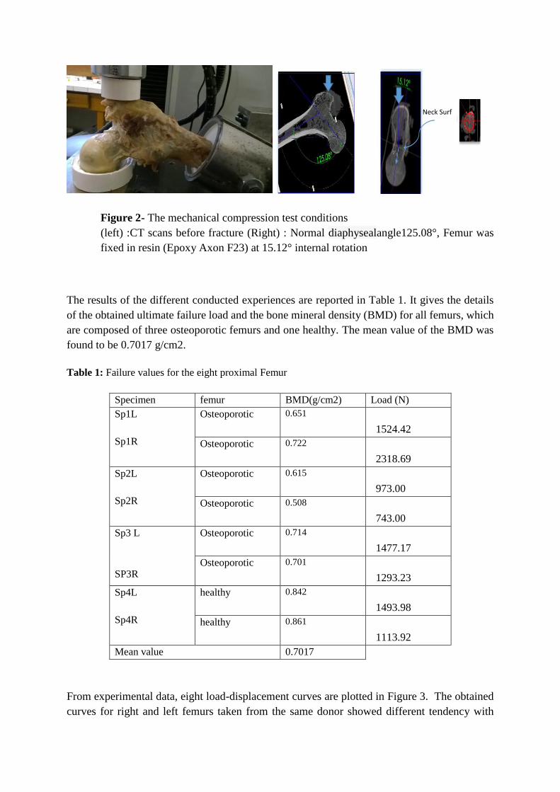
Figure 2- The mechanical compression test conditions

(left) :CT scans before fracture (Right) : Normal diaphysealangle125.08°, Femur was

fixed in resin (Epoxy Axon F23) at 15.12° internal rotation

The results of the different conducted experiences are reported in Table 1. It gives the details

of the obtained ultimate failure load and the bone mineral density (BMD) for all femurs, which

are composed of three osteoporotic femurs and one healthy. The mean value of the BMD was

found to be 0.7017 g/cm2.

Table 1: Failure values for the eight proximal Femur

Specimen femur BMD(g/cm2) Load (N)

Sp1L

Sp1R

Osteoporotic 0.651

1524.42

Osteoporotic 0.722

2318.69

Sp2L

Sp2R

Osteoporotic 0.615

973.00

Osteoporotic 0.508

743.00

Sp3 L

SP3R

Osteoporotic 0.714

1477.17

Osteoporotic 0.701

1293.23

Sp4L

Sp4R

healthy 0.842

1493.98

healthy 0.861

1113.92

Mean value 0.7017

From experimental data, eight load-displacement curves are plotted in Figure 3. The obtained

curves for right and left femurs taken from the same donor showed different tendency with

Neck Surf

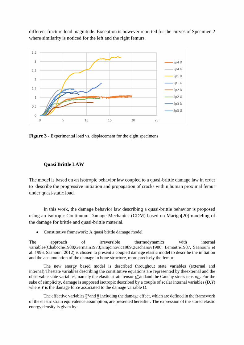
different fracture load magnitude. Exception is however reported for the curves of Specimen 2

where similarity is noticed for the left and the right femurs.

Figure 3 - Experimental load vs. displacement for the eight specimens

Quasi Brittle LAW

The model is based on an isotropic behavior law coupled to a quasi-brittle damage law in order

to describe the progressive initiation and propagation of cracks within human proximal femur

under quasi-static load.

In this work, the damage behavior law describing a quasi-brittle behavior is proposed

using an isotropic Continuum Damage Mechanics (CDM) based on Marigo[20] modeling of

the damage for brittle and quasi-brittle material.

• Constitutive framework: A quasi brittle damage model

The approach of irreversible thermodynamics with internal

variables(Chaboche1988;Germain1973;Krajcinovic1989;;Kachanov1986; Lemaitre1987, Saanouni et

al. 1996, Saanouni 2012) is chosen to present a coupled damage elastic model to describe the initiation

and the accumulation of the damage in bone structure, more precisely the femur.

The new energy based model is described throughout state variables (external and

internal).Thestate variables describing the constitutive equations are represented by theexternal and the

observable state variables, namely the elastic strain tensor 𝜀𝑒andand the Cauchy stress tensor𝜎. For the

sake of simplicity, damage is supposed isotropic described by a couple of scalar internal variables (D,Y)

where Y is the damage force associated to the damage variable D.

The effective variables εeand σ including the damage effect, which are defined in the framework

of the elastic strain equivalence assumption, are presented hereafter. The expression of the stored elastic

energy density is given by:

0

0,5

1

1,5

2

2,5

3

3,5

0 5 10 15 20 25

Sp4 D

Sp4 G

Sp1 D

Sp1 G

Sp2 D

Sp2 G

Sp3 D

Sp3 G

ρψ(εe, D) =1

2(1 − D)εe: A: εe + ψ⏞ (D)(5)

According to the Marigo hypothesis:ψ⏞ (D) = 0 dire ce que c’est ψ⏞

Where A is thesymmetric fourth-rank tensor of elastic properties of the virgin (not affected by

damage) material, which in the isotropic case can be written in terms of the well-known Lame’s

constantsand according to:

A 1 1 2 1= +

= 𝐸

(1 − 2); =

𝐸

(1 + )(1 − 2)

Where 1 is the second-rank identity (Krönecker) tensor while 1 is a fourth-rank unit tensor.

According to the theory of Marigo, the global energy depends only on the two state variables

namely the elastic strain tensor and the damage.

The state laws𝝈and Y,are classically derived from the state potential are obtained from the freeenergy

by:

σ = ρ∂ψ

∂εe = (1 − D)A: εe(6.1)

A = ρ∂2ψ

∂2εe > 0 (6.2)

σ = (1 − D) ( 1 1 + 2 1 ) : εe(6.3)

𝑌 = −𝜌𝑑𝜓

𝑑𝐷=

1

2𝜀𝑒: 𝐴: 𝜀𝑒(7)

The damage criterion(or damage yield function) is described by Y:

f(Y, D) = Y −1

2Y0 − mD

1

s = 0 (8)

where 𝑌0,s and m are material parameters. The parameters s and m are related to the damage

“hardening” of the material. It is here to be noticed that the damage yield function Eq.(8) can describe

the initiation of micro-cracks starting from undamaged state (D=0).

In the present model, the dissipation potential 𝝋 is reduced to the yield function f according

to the associative theory:

φ = f = Y −1

2Yo − mD

1

s = 0(9)

The damage evolution equation derived from the dissipation potential is:

φ = 0 ⇔∂φ

∂YY +

∂φ

∂DD = 0 (10)

For this approach, the coupling between damage and elasticity is completed with the following

damage evolution law.

�� = 𝑠

𝑚

��

𝐷1−𝑠

𝑠

(11)

With:

e eY : := & &(12)

According to Eq. (6.3), when damage increases by Eq. (11), then the stress tensor decreases due

to the decrease of the Lame’s constants (i.e. the Young’s Modulus).

Solving the non linear problem described by Eqs (6)-(12) in order to determine the unknowns

of the problem is performed through an approximation of these variables in total time interval 𝐼𝑡 =

[t0, tf] = ⋃ [tn, tn+1 = tn + ∆t]Ntn=0 ,t being the increment between two successive time steps. This

approximation is done for every integration point related to every finite element.

Thus knowing the initial variables at tn, the discretized problem is solved giving the final

solution at the final time tn+1.The discretization leads to the following expressions of the problem

variables at tn+1=tn+t, the end of the step time:

σn+1 = (1 − Dn+1) (tr εen+1

. I + 2εen+1

)(13)

εen+1

= εen

+ Δεen(14)

𝑌𝑛+1 =1

2𝜀𝑒

𝑛+1: 𝐴: 𝜀𝑒

𝑛+1(15)

fn+1 = Yn+1 −1

2Y0 − mDn+1

1

s = 0 (16)

From this last equation, the “admissible” value of the damage variable is deduced as:

𝐷𝑛+1 = ⟨𝑌𝑛+1 −

1

2𝑌0

𝑚⟩𝑠 (17)

In this isotropic damage model, some remarks can be made:

• If the scalar variable describing damage is zero (D=0.0), then the material state is

described by the classical isotropic elastic model.

If the fracture condition of the critical value (D=1.0) is reached, then the material point

is declared as fully damaged and the following value is assigned to D in that point

D=0.999.

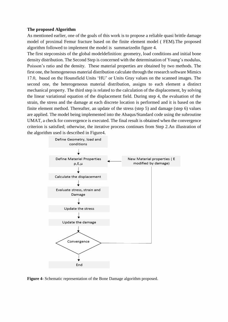
The proposed Algorithm

As mentioned earlier, one of the goals of this work is to propose a reliable quasi brittle damage

model of proximal Femur fracture based on the finite element model ( FEM).The proposed

algorithm followed to implement the model is summarizedin figure 4.

The first stepconsists of the global modeldefinition: geometry, load conditions and initial bone

density distribution. The Second Step is concerned with the determination of Young’s modulus,

Poisson’s ratio and the density. These material properties are obtained by two methods. The

first one, the homogeneous material distribution calculate through the research software Mimics

17.0, based on the Hounsfield Units ‘HU’ or Units Gray values on the scanned images. The

second one, the heterogeneous material distribution, assigns to each element a distinct

mechanical property. The third step is related to the calculation of the displacement, by solving

the linear variational equation of the displacement field. During step 4, the evaluation of the

strain, the stress and the damage at each discrete location is performed and it is based on the

finite element method. Thereafter, an update of the stress (step 5) and damage (step 6) values

are applied. The model being implemented into the Abaqus/Standard code using the subroutine

UMAT, a check for convergence is executed. The final result is obtained when the convergence

criterion is satisfied; otherwise, the iterative process continues from Step 2.An illustration of

the algorithm used is described in Figure4.

Figure 4- Schematic representation of the Bone Damage algorithm proposed.

In the present work and for the sake of comparison, bone was modeled as an isotropic material

with two mechanical properties (Young modulus E (MPa)) estimated through two different

methods. These techniques were used in previous works. Indeed, most of these studies, adopted

a non homogenous elastic modulus related the density. As examples of these works we can

recallmorgan E.F et al. [21], Keyak J.H. [22], Ariza O. [23], Pithioux et al. [24] and Haider et

al.[7]. However, some researchers adopted the method based on the assumption that the elastic

modulus is homogenous and a function of volume fraction (BV/TV) . These studies can found

in the references (Hambli R. et al. [25] and Varga P. et al. [13]). We will recall here after these

two methods of E determination.

Method 1 : Non homogenous Young Modulus

The first method using the following expression gives a varying Young modulus (E) related to

the bone apparent density ρ such as defined by Kaneko et al. [26],

E1= 2000 ρ1.89 (1)

ρ: apparent density (g/cm3)

This method is based on a phenomenological law and allows to assign to each element a distinct

mechanical property using a direct correlation between apparent density and Young Modulus.

In the end, a heterogeneous material distribution was obtained.

Method 2 : Homogenous Young Modulus

For method 2, homogenization techniques were considered, allowing to obtain a homogeneous

material distribution. The following relationship is proposed by Hernandez et al. [27]:

E2 = 84370 (𝐵𝑉

𝑇𝑉)

2.58

(2)

BV/TV:bone volume/total volume fraction;

Thirty-two numerical computations based on eight Femurs reconstructions are validated

through a comparison of the experimental crack localization and of the estimated failure loads.

The material properties E and ρ are summarized in Table 2. Poisson ratio is set at 0.3 based on

the work of [28,29,30].

Table 2. Material Properties for height specimens

Femur Strength

Load (N)

Density Young

Modulus (Mpa)

Method 1

Young

Modulus(Mpa)

Method 2

Poisson

ratio

Sp1 G 1524.42 0.28 – 2.45 121 – 14475

3777

0.3

D 2318.69 0.25 – 2.46 103 - 14552

Sp2 G 973 0.47 – 2.44 384– 14293

D 743 0.35 – 2.42 199 - 13991

Sp3 G 1477.17 0.41-2.41 292-13905

D 1293.23 0.32-2,46 161-14469

Sp4 G 1493.98 0.34-2.458 185-14526

D 1113.92 0.31-2.45 151-14405

Simulations

• Boundary and Loading conditions

The numerical validation is conducted with the boundary condition and load case

representing the experimental conditions (Figure 5). The load was applied on femoral

Greater trochanter reproducing the sideway fall case, whereas the femoral head and the

lower surface were constrained. During the conducted computations, the stiffness of

elements degrades gradually as damage increase, and the crack is modeled as the region of

elements whose stiffness has been reduced to near zero.

Figure 5 -The mechanical compression test conditions (Left) and BCs applied to the FE

model(Right)

Results

The general purpose of this work is to compare the prediction of the damage localization

as well as of the ultimate fracture load for different specimens tested experimentally for two

meshing model, linear mesh with linear tetrahedral elements (C3D4), and nonlinearmesh with

quadratic tetrahedral elements (C3D10) (six degrees of freedom per node which are the three

displacements and the three rotations). The ultimate strength load value obtained

experimentally was applied for the two methods which are based on two different approaches

to estimate the Young modulus as previously presented. The analysis details the fracture load

and the localized damaged zones dependency on the young modulus estimation as well as the

linearity or not of the meshing.

LOAD

B.C

The 32 correlations between the experimental and FE computed fracture loads for the four

studied cases are exposed in Figure 6. In summary and as it appears in Figure 6 (D), the

numerical computations based on the use of an homogeneous material distribution with a

nonlinear mesh, present a good agreement with the experimental data (fracture load magnitude)

with the best correlation ( R²= 0.825). For the other cases (Figure 6 (A),(B) and(C)) ,

correlations are weak and lower than 0.356 .

A B

C D

Figure 6- Numerical fracture loads (KN) and the relative error based on a comparison with the

experimental data for the eight cases (right and left femurs) computed with E1 and E2: (A) Method1-

Linear Mesh; (B) Method1-NonLinear Mesh; (C) Method2-Linear Mesh; (D) Method2-NonLinear

Mesh

In Table 3 the relative errors between the experimental and the computed fracture loads are

reported. The best results is obtained for the case where we use Young modulus E related to the

microarchitecture parameter (method 2) for the non-Linear mesh. The fracture load error

average was found to be 6.49 %.

Table 3. Relative Error´s summary

Linear Model Non Linear Model

Relative Error (%) Average (%) Relative Error (%) Average (%)

Method 1 15.6 - 59.7 41.63 6.5 - 52.2 23.95

Method 2 4.7 - 24 13.31 0.4 - 18.4 6.49

The propagations of the cracks and the distribution of the quasi-brittle damage of the

eight femurs are plotted in Figure7

The results of the numerical computations gave two different crack localizations based

on the choice of the elastic property. Indeed, the FE simulations performed with the method

2,showed a femoral neck (transcervical) fracture, the crack is initiated locally at the superior

surface of femoral neck. Then the crack continues to grow, resulting a separation of the

proximal femur. However, in this case the damage surface corresponded to the fracture surface

observed in the experience, differently from the first method, where fracture occurred in the

Greater trochanter. The same observations are obtained for the two femurs (right and the left)

for the all studied femurs.

The crack localizations for the two models linear and nonlinear are quasi similar, except that in

the nonlinear modeling case, the entire femur is affected by the damage as shown in Figure 7

for the SP4 R and SP4 L. These observations are very interesting since as it has been related in

previous studies, nonlinear meshing can be computationally expensive (cpu).

Linear Meshing Model Nonlinear Meshing Model

Femur Method 1 Method 2 Method 1 Method 2

Posterior

View

Anterior

View

Posterior

View

Anterior

View

Posterior

View

Anterior

View

Posterior

View

Anterior

View

SP1 R

SP1 L

SP2 R

SP2 L

SP3 R

SP3 L

SP4 R

SP4 L

Figure 7 - Predicted fracture pattern from different view and quasi-brittle damage distribution.

Special attention will now be paid to one of the specimens presented in the previous overall

results. The final goal is to better underlined the quantitative and qualitative results obtained for

the eight specimens. The specimen chosen is the one named SP3R. It is a representative sample

of all the studied specimens. We begin by a comparison between the experimental and

numerical behavior curves (with linear and non linear meshing) obtained during the simulation

of the sideways fall.

This comparison which is illustrated in Figure (8) shows a good simulation between

experimental and numerical results. Besides, the nonlinear case shows the best agreement with

experimental curve, as well as a sharp drop in force during failure.

Figure 8 -Predicted and experimental force-displacement curves of the present FE model Sp 3R for the

Method 2, Linear and nonlinear mesh

Figure 9 shows a validation between the numerical for both cases of meshing /linear and

nonlinear) and experimental results of the fracture pattern, and clearly demonstrate that the

fracture line is located in the neck region

Also, Figures9a and 9b show that regardless of the choice of type of meshing (linear or

nonlinear), we obtain fracture localizations similar to the ones obtained experimentally (Figure

9c).

In conclusion, this validation of load fracture and localization proves the performance of the

adopted numerical method, which is formulated in the CDM framework. It also clearly

demonstrated that the result is affected by the choice of the type of mesh (linear or nonlinear)

whereas the damage pattern does not depend on this parameter.

0

0,2

0,4

0,6

0,8

1

1,2

1,4

1,6

0 2 4 6 8 10 12

Frac

ture

Lo

ad (

KN

)

Displacement

Experiment(StudiedFemur)Present Model(NonlinearMesh)Present Model(Linear Mesh)

LinearMesh

NonlinearMesh

a b c

b a c

Linear MeshModel Nonlinear Mesh

Model

Experimental

Femur AnteriorView AnteriorView AnteriorView

SP3 R

SP3 L

Figure 9-Qualitative evaluation of the FE based fracture pattern prediction, for linear mesh (a) and

nonlinear mesh (b) by comparing with experimental compression-test photos (c) showing the anterior

View for Specimen 3 Right and Left adopting method 2.

Discussion

The aim of the present study was to implement a comparative study based on 32 simulations,

using a linear and nonlinear mesh to show that the results are improved when a nonlinear mesh

is used. As a first remark, we can say that the predicted force-displacement curve shows the

same trend as the one observed experimentally. Regarding the relative error, the average error

is about 6.49% with a very good fracture pattern predictions for all specimens, compared to

previous works presetend by Haider I.T and al[7]. The average percentage errors of predicted

fracture load was about 9.6% and peak error of only 14%. However, they have recalled that

the average errors found in previous studies was less than the previously published studies

which are from 10% to 20% [7].

In general, we found statistically moderate correlations between the experimentally and

computationally results using a homogeneous young modulus (method2) and using nonlinear

meshing(R²=0.825). However, no correlation was found between experimental and FE model

for the heterogeneous young modulus distribution using the linear meshing and for two meshing

model of the heterogeneous method. Regarding the localization issue, we found that in general,

the experimental bone failure locations agreed with the locations of the FE for the method 2.

Referring to the Garden Classification [31], different fracture can be observed experimentally

and the numerically, depending on the femoral geometry, the material properties and the

boundary conditions. In this work, the fracture patterns correspond to a Transervical neck

fracture with stage II (Complete fracture with minimal or no displacement from anatomically

normal position) of the Garden classification. To the best of the author’s knowledge, this is the

first time a comparison of linear and nonlinear meshing was established for the prediction of

femoral fracture. Although we find the results encouraging, one limitation of this study is

related to the mesh sensitivity, which should adopt an effective technique to better predict

fracture load, fracture pattern, and fracture initiation independently of mesh density. Overall,

the FE model precision was demonstrated by comparing the simulation results to the

experimental results for each specimens.

Conclusion

The purpose of this work was to develop and validate a simple FE model based on continuum

damage mechanics in order to simulate the complete force–displacement curve of femur failure.

Femoral fracture load was predicted using a quasi brittle-damage FE model for four studied

cases, combining homogeneous and heterogeneous material distribution with a linear and

nonlinear mesh. The obtained results show a strong linear relationship between FE predicted and

experimentally measured fracture load (R2= 0.825) in the case combining homogenous material

distribution with non linear mesh. Furthermore, all eight cadaveric specimens present a similar

failure locations between the experimental and the FE simulation, when the method 2 is

adopting.

The presented FE model shows strong correlations between experimental and numerical values

however is spurious mesh sensitivity. The size of the damaged region corresponds to the size

of the mesh used to solve the problem. As the mesh is refined, the size of the damaged region

Despite limitations of our study, cited above, the relatively low average error in the fourth case

suggests that this FE methodology may be useful in helping the surgeon choose a patient-

specific treatment, and allowing them to make the right decision before the surgery by

evaluating the risk factor from the fracture pattern.

Acknowledgements

The contribution of Saint Marguerite hospital radiology team specially P. Champsaur, T.

Lecorroller, and D. Guenou is gratefully acknowledged.

References

1. Briot K, Cortet B, Thomas T, Audran M, Blain H, Breuil L.C, Chapurlat R, Fardellone P, Feron

J.M, Gauvain J.B, Guggenbuhl P, Kolta S, Lespessailles E, Letombe B, Marcelli C, Orcel

P,Seret P, Trémollière F, Roux C,« Actualisation 2012 des recommandations françaises du

traitement médicamenteux de l´ostéoporose post-ménopausique », Revue du rhumatisme 79

(2012), p 264-274.

2. Tellache M, Pithioux M , Chabrand P , Hochard C , Champsaur P and LeCorroller T. Etude

expérimentale de la rupture osteoporotique du col femoral.2007. 18ème Congrès Français de

Mécanique, Grenoble, 27-31 août 2007

3. Tellache M, Pithioux M , Chabrand P and Hochard C (2009) Femoral neck fracture prediction

by anisotropic yield criteria, European Journal of Computational Mechanics/Revue Européenne

de Mécanique Numérique, 18:1, 33-41Tellache M et al, Euro J of Computational Mechanics,

18:33-41, 2009.

4. Curtis EM, Moon RJ, Harvey NC, Cooper C. 2017. The impact of fragility fracture and

approaches to osteoporosis risk assessment worldwide. Bon(2017). doi:

10.1016/j.bone.2017.01.024

5. Bettamer A, Hambli R, Allaoui S and Almhdie-Imjabber A,2015, “Using visual image

measurements to validate a novel finite element model of crack propagation and fracture

patterns of proximal femur”. Computer Methods in Biomechanics and Biomedical Engineering:

Imaging & Visualization, DOI: 10.1080/21681163.2015.1079505

6. Viceconti M, Taddei F, Cristofolini L, Martelli S, Falcinelli C, Schileo E ,2012, “Are

spontaneous fractures possible? An example of clinical application for personalised, multiscale

neuro-musculo-skeletal modelling”. Journal of Biomechanics 45 (2012), 421–426

7. Haider I T, Goldak J, Frei H, 2018, “Femoral fracture load and fracture pattern is accurately

predicted using a gradient-enhanced quasi-brittle finite element model”. Medical Engineering

and Physics 0 0 0: 1–8

8. MARCO M, GINER E, LARRAINZAR R, CAEIRO J.R, and MIGUELEZ M.H,2017,

“Numerical Modelling of Femur Fracture and Experimental Validation Using Bone Simulant”,

Annals of Biomedical Engineering DOI: 10.1007/s10439-017-1877-6 .

9. Enns-Bray W.S, Owoc J.S, Nishiyama K.K, Boyd S.K, 2014, “Mapping anisotropy of the

proximal femur for enhanced image based finite element analysis”. Journal of Biomechanics

47(2014), 3272–3278

10. Bettamer A, Hambli R, Berkaoui A, Allaoui S, 2011, “Prediction of proximal femoral fracture

by using Quasi-brittle damage with anisotropic behaviour model”, 2nd International Conference

on Material Modelling, Aug 2011, PARIS, France. pp.ID269, 2011. <hal-00772663>

11. Lekadir K, Hazrati-Marangalou J, Hoogendoorn C, Taylor Z, vanRietbergen B, Frangi A.F,

2015, “Statistical estimation of femur micro-architecture using optimal shape and density

predictors”. Journal of Biomechanics 48(2015), 598–603

12. Zagane M.S, Benbarek S, Sahli A, Bouiadjra B.B and Boualem S, 2016, “Numerical simulation

of the femur fracture under static loading”. Structural Engineering and Mechanics, Vol. 60, No.

3 (2016) 405-412 DOI: http://dx.doi.org/10.12989/sem.2016.60.3.405

13. Vargaa P, Schwiedrzik J, Zysset Ph.K, Fliri-Hofmanna L , Widmera D, Gueorguiev B, Blauth

M, Windolf M ,2016, “Nonlinear quasi-static finite element simulations predict in vitro strength

of human proximal femora assessed in a dynamic sideways fall setup”, Journal of the

mechanical behavior of biomedical materials 57 , 116-127

14. Nawathe S, Yang H, Fields A.J,.Bouxsein M.L, Keaveny T.M, 2015, “Theoretical effects of

fully ductile versus fully brittle behaviors of bone tissue on the strength of the human proximal

femur and vertebral body”. Journal of Biomechanics 48(2015), 1264–1269

15. Schmidt J, Henderson A, Ploeg H, Deluzio K, Dunbar M. Finite element analysis of stem

dimensions in a revision total knee arthroplasty using visible human computed tomography

data.2006.

16. AbdulKadir M.R,. Finite Element Model Construction.2014. Computational Biomechanics of

the Hip Joint SpringerBriefs in Computational Mechanics, DOI: 10.1007/978-3-642-38777-

7_2.

17. Dieter H.P, Zysset P.K, « A comparaison of enhanced continuum FE with micro FE models of

human vertebral bodies», Journal of Biomechanics 42 , 2009, p 455-462.

18. Nakhli Z, Ben Hatira F, Pithioux M, Chabrand P. DEPENDENCE DE LA MODELISATION

PAR ELEMENTS FINIS DU FEMUR HUMAIN DE LA RECONSTRUCTION

TRIDIMENSIONNELLE. International Congress / Congrès International Design and

Modelling of MechanicalSystems Conception et Modélisation des Systèmes Mécaniques 27 -

29 _ March / Mars 2017, Hammamet – Tunisia / Tunisie

19. Le Corroller T, Halgrin J, Pithioux M, Guenoun F, Chabrand P, Champsaur P. Combination of

texture analysis and bone mineral density improves the prediction of fracture load in human

femurs .2011 . Osteoporos Int (2012) 23 :163-169 .

20. Marigo JJ: Formulation of a damage law for an elastic material. Comptes Rendus, Serie II-

Mécanique, Physique, Chimie, Sciences de la Terre1981, 1390-1312.

21. Morgan E.F., Bayraktar H.H., Keaveny T.M., 2003. Trabecularbonemodulus– density

relationships depend on anatomic site.J.Biomech.36,897–904.

22. Keyak J.H , Improved prediction of proximal femoral fracture load using nonlinear finite

element models, 2001 Medical Engineering & Physics 23 (2001) 165–173

23. Ariza O, Gilchrist S, Widmer R.P, Guy P, Ferguson S.J , Cripton P.A, Helgason B. Comparison

of explicit finite element and mechanical simulation of the proximal femur during dynamic

drop-tower testing.2015. Bone 81 (2015) 122–130

24. Pithioux M, Chabrand P, Hochard CH and Champsaur P. Improved Femoral Neck fracture

predictions using anisotropic failure criteria models. 2011. Journal of Mechanics in Medicine

and Biology Vol. 11, No. 5 (2011) 1333–1346

25. Hambli R, Bettamer A, Allaoui S. Finite element prediction of proximal femur fracture pattern

based on orthotropic behaviour law coupled to quasi-brittle damage. 2012. Medical Engineering

& Physics 34 , 202– 210

26. Kaneko TS, Bell JS, Pejcic MR, Tehranzadeh J, Keyak JH. Mechanical properties, density and

quantitative CT scan data of trabecular bone with and without metastases. 2004. Journal of

Biomechanics.37: 523–530.

27. Hernandez CJ, Beaupre G S, Keller TS, Carter DR. The influence of bone volume fraction

and ash fraction on bone strength and modulus. Bone, 29(1):74–78, 2001.

28. Jundt G, «Modèles d´endommagement et de rupture des matériaux biologiques». Thèse, 2007,

p 193

29. Currey JD: The effect of porosity and mineral content on theYoung’s modulus elasticity of

compact bone.JBiomech 1988, 21:131–139.

30. Carter DR, Hayes WC: The compressive behavior of bones as a two-phase porous structure. J

Bone Joint Surg Am 1977, 59:954–962.)

31. Frandsen P.A, Andersen E, Madsen F, Skjodt T. Garden´s Classification of femoral Neck

Fractures. 1988. The journal of bone and joint surgery Vol 70-B. No.4: 588-590