KHALID JAVED A Thesis In - Concordia University · i behavior of sensitive clay subjected to static...
202
i BEHAVIOR OF SENSITIVE CLAY SUBJECTED TO STATIC AND CYCLIC LOADING KHALID JAVED A Thesis In THE DEPARTMENT OF BUILDING, CIVIL AND ENVIRONMENTAL ENGINEERING Presented in Partial Fulfillment of the Requirements For the Degree of Doctor of Philosophy CONCORDIA UNIVERSITY Montreal, Quebec, Canada February 2011 Khalid Javed
Transcript of KHALID JAVED A Thesis In - Concordia University · i behavior of sensitive clay subjected to static...

i
BEHAVIOR OF SENSITIVE CLAY SUBJECTED TO
STATIC AND
CYCLIC LOADING
KHALID JAVED
A Thesis
In
THE DEPARTMENT OF BUILDING, CIVIL AND ENVIRONMENTAL
ENGINEERING
Presented in Partial Fulfillment of the Requirements
For the Degree of Doctor of Philosophy
CONCORDIA UNIVERSITY
Montreal, Quebec, Canada
February 2011
Khalid Javed

ii
CONCORDIA UNIVERSITY
SCHOOL OF GRADUATE STUDIES
This is to certify that the thesis prepared
By: Mr. Khalid Javed
Entitled: Behavior of Sensitive Clay Subjected to Static and Cyclic Loading
and submitted in partial fulfillment of the requirements for the degree of
Doctor of Philosophy
complies with the regulations of this University and meets the accepted standards with respect to
originality and quality.
Signed by the final examining committee:
Chair
External Examiner
External to Program
Examiner
Examiner
Thesis Supervisor
Approved by
Chair of Department or Graduate Program Director
June, 2011
Dr. Robin Drew
Dean of Faculty
Dr. B. Jaumard
Dr. A. Zsaki
Dr. O. Pekau
Dr. A.M. Hanna
Dr. Hesham El Naggar
Dr. G. Vatistas
Dr. M.Elektorowicz

iii
ABSTRACT
Sensitive clay is the type of clay, which loses its shear strength when it is subjected to cyclic
loading. High-rise buildings, towers, bridges etc., founded on sensitive clays and subjected to
overturning moment are usually suffer from a steady reduction of the bearing capacity of their
foundations and accordingly the safety factor. Cyclic loading of foundation on sensitive clay
during the undrained period may lead to quick clay condition and catastrophic failure of the
structure.
In the literature, governing parameters are listed as: cyclic deviator stress, pore water pressure,
axial strain, pre-consolidation pressure, confining stress, initial degree of saturation, water
content, liquidity index and the number of cycles. The present study has introduced the
governing parameters in two categories; namely physical and mechanical as a function of
sensitivity number of the clay material. A well planned experimental investigation was
conducted to examine the effect of these governing parameters during the undrained and the
drained periods of sensitive clay subjected to static or cyclic loadings. The soil samples, known
as “Champlain clay” were obtained from the city of Rigaud, Quebec (Canada). Consolidation
tests, static and cyclic undrained and drained triaxial tests were performed on representative
samples of this clay.
Tests were conducted to identify the role of the key parameters governing this complex behavior
during the drained and the undrained periods. The study examined individually the effect of
cyclic loading, deviator stress, frequency, pre-consolidation pressure/OCR, and the confining
pressure during the drained and undrained conditions. Absence or presence of the matric suction
in fully saturated or partially saturated clay, effect of sensitivity number and liquidity index were
also examined.
iv
Based on the results of the present experimental investigation, a hypothetical model was
introduced to explain the process of shear strength reduction for the case of static and cyclic
loading of sensitive clay subjected to cycling loading. The model was capable to define the term
remolding agent or degree of remolding, the reduction in shear strength due to remolding. The
increase in the water content is identified as the most critical or intrinsic shear strength for
sensitive clay.
The present study used the “Modified Cam Clay Model” to predict the factor of safety for a
foundation on sensitive clay subjected to cyclic loading as function of the physical and
mechanical parameters. A design procedure is developed to determine the safe zone for the
undrained and drained responses, within which a combination of the cyclic deviator stress and
the number of cycles for a given soil/loading/site conditions can achieve a quasi-elastic resilient
state without reaching failure. The proposed design procedure is applicable to all regions around
the world, where sensitive clays can be found. Furthermore, this procedure can be adopted to
examine the conditions of existing foundations built on sensitive clay at any time during its
lifespan.

v
Acknowledgement
I owe my most sincere gratitude to Al-mighty Allah who has been the source of my entire
initiative and accomplishment required to fulfill this stupendous task.
My most fervent thanks are due to my mother whose prayers enabled me to see this day.
I pray to Allah for my late father Abdul Shakur to grant him paradise and elevate his level in the
life hereafter. He was a competent civil engineer and a man-of-peace. Whatever achievements I
have in my life are the result of his training.
The entire credit of the accomplishment of this research goes to Prof. Dr. Adel Hanna, my thesis
director, whose technical guidance, deep involvement, personal interest and untiring assistance
enabled me to present this work today.
The financial support provided by the Natural Sciences and Engineering Council of Canada is
acknowledged and highly appreciated.
I am also thankful to my wife and kids for unexhausted support and encouragement.

vi
Contents
Chapter 1 .................................................................................................................................................................... 19
Introduction ................................................................................................................................................................. 19
Chapter 2 .................................................................................................................................................................... 29
Literature Review ........................................................................................................................................................ 29
2.1 Discussion ...................................................................................................................................................... 48
2.2 Problem Definition ........................................................................................................................................... 52
Chapter 3 .................................................................................................................................................................... 63
Experimental Investigation .......................................................................................................................................... 63
3.1 Sample Source ................................................................................................................................................. 63
3.2 Methods of Acquiring Samples ....................................................................................................................... 63
3.3 Types of Selected Clays ................................................................................................................................... 65
3.4 Grouping of Samples and Type of Tests conducted ........................................................................................ 65
3.5 Determination of Physical and Index Properties .............................................................................................. 66
3.6 Conventional Consolidation Test ..................................................................................................................... 68
3.7 Sensitivity Number .......................................................................................................................................... 69
3.8 Triaxial Testing ................................................................................................................................................ 70
3.8.1 Triaxial Test Principle and Program ........................................................................................................... 71
3.8.2 Setting up the Triaxial Apparatus for Static and Cyclic Triaxial Tests..................................................... 71
3.9 Calibration of various Instruments and Transducers used in Triaxial Testing ................................................... 72
3.9.1 Calibrating Submersible Load Cell ............................................................................................................. 73
3.9.2 Calibrating LVDT ....................................................................................................................................... 73
3.9.3 Calibrating Pore Pressure Transducer ......................................................................................................... 74
3.10 Programming the Agilent Data Acquisition System ........................................................................................ 74
3.11 Experimental Program Layout ......................................................................................................................... 76
3.12 Static Triaxial Compression Test (Undrained) ................................................................................................ 77
3.13 Cyclic Triaxial Compression Test ................................................................................................................... 78
3.14 Discussion ........................................................................................................................................................ 79
Chapter 4 .................................................................................................................................................................. 105
Analysis and Theory .............................................................................................................................................. 105
4.1 Static Triaxial Tests .................................................................................................................................... 106
4.2 Cyclic Triaxial Tests ................................................................................................................................... 109
4.3 Drained and Undrained Triaxial Compression Tests .................................................................................. 111
4.4 Effect of Undisturbed and Remolded Samples ........................................................................................... 112
4.5 Effect of over-consolidation ratio ............................................................................................................... 113
4.6 Effect of frequency ..................................................................................................................................... 114
4.7 Effect of confining pressure ........................................................................................................................ 115

vii
4.8 Effect of Sensitivity Number and Liquidity Index (IL) ............................................................................... 116
4.9 Effect of initial degree of saturation ........................................................................................................... 118
4.10 Effect of Cyclic Deviator Stress ................................................................................................................. 121
4.11 Effect of number of cycles .......................................................................................................................... 125
4.12 Theoretical Application of Experimental Data ........................................................................................... 126
4.12.1 Hypothetical Model ......................................................................................................................... 127
4.12.2 Adapting Modified Cam Clay Model for Analyzing Behavior of Sensitive Clay Subjected to Cyclic
Loading ......................................................................................................................................................... 129
4.12.3 Effect of frequency ........................................................................................................................ 135
4.12.4 Modeling the Role of Physical Parameters .................................................................................... 136
4.12.5 Effect of Degree of Saturation ...................................................................................................... 137
4.13 Safe Zone .................................................................................................................................................. 139
4.14 Discussion ................................................................................................................................................. 141
Chapter 5 .................................................................................................................................................................. 181
Conclusions and Recommendations ...................................................................................................................... 181
5.1 Research Contribution .............................................................................................................................. 181
5.2 Limitations of Research ........................................................................................................................... 182
5.3 Conclusions .............................................................................................................................................. 183
5.4 Recommendation for the future work ...................................................................................................... 185
REFERENCES .......................................................................................................................................................... 186
LIST OF TABLES
Table 2.1: General Properties of Investigated Soils ..................................................................................................... 53
Table 3.1 Grouping, type of sample, test conducted & parameters obtained .............................................................. 83
Table 3.2: Summary of index property test results ..................................................................................................... 85
Table 3.3: Summary of consolidation test ................................................................................................................... 86
Table 3.4 Summary of unconfined triaxial tests ......................................................................................................... 87
Table 3.5: Calibration of submersible load cell 5 kN .................................................................................................. 88
Table 3.6 Calibration for LVDTs ............................................................................................................................... 88
Table 3.7: Calibration for pore water pressure transducer ........................................................................................... 89
Table 3.8 Nature of tests conducted on each type of sensitive clay (A, B, C and D) .................................................. 90
Table 3.9 Summary of static triaxial compression test ................................................................................................ 91
Table 3.10 Summary of cyclic triaxial compression test ............................................................................................. 92

viii
LIST OF FIGURES
Figure 1.1: Approximate extent of sensitive clay deposition;...................................................................................... 24
Figure 1.2: Cyclic loading due to offshore waves (After Reilly and Brown, 1991) .................................................... 25
Figure 1.3: Cyclic loading due to wind (After Reilly and Brown, 1991) .................................................................... 25
Figure 1.4: Cyclic loading due to construction (After Reilly and Brown, 1991) ......................................................... 26
Figure 1.5: Cyclic loading due to machines (After Reilly and Brown, 1991) ............................................................. 26
Figure 1.6: Cyclic loading due to traffic (After Reilly and Brown, 1991) ................................................................... 27
Figure 1.7: Micrograph of a horizontal cleavage surface in undisturbed and desiccated St. Vallier clay. (After McK
et al. 1973) ................................................................................................................................................................... 27
Figure 1.8: Micrograph of a horizontal cleavage surface in disturbed and desiccated St. Vallier clay. (After McK et
al. 1973) ....................................................................................................................................................................... 28
Figure 2.1: Cyclic failure data for San Francisco Bay Mud (Houstan and Hermann, 1979) ....................................... 54
Figure 2.2: Cyclic strength contours for San Francisco Bay Mud ............................................................................... 54
Figure 2.3: Ratio of modified to static shear strengths versus strain rate (Procter and Khaffaf, 1984) ..................... 55
Figure 2.4: Frequency response of cyclic stress ratio (cu) (Procter and Khaffaf, 1984) ........................................... 55
Figure 2.5: Frequency response of modified cyclic stress ratio (c-u) ........................................................................ 56
Figure 2.6: Change of undrained strength ratio, normalized to undrained strength ratio at strain rate for all
investigated clays (Lefebyre and LeBoeuf, 1987) ....................................................................................................... 56
Figure 2.7: Cyclic yield strength versus number of cycles .......................................................................................... 57
Figure 2.8: Cyclic stress ratio-pore pressure relationship for different numbers of cycles (Ansal and Erken, 1989) .. 57
Figure 2.9: Slope of pore water pressure lines versus number of cycles ..................................................................... 58
Figure 2.10: Comparison of shear strain of one-dimensionally consolidated and remolded samples (Ansal and Erken,
1989) ............................................................................................................................................................................ 58
Figure 2.11: Comparison of pore water pressure of one-dimensionally consolidated and remolded samples (Ansal
and Erken, 1989).......................................................................................................................................................... 59
Figure 2.12: Interrelationship between sensitivity and liquidity index for natural clays ............................................. 59
Figure 2.13: variation of remolded undrained strength cu with ................................................................................... 60
Figure 2.14: Mohr's circles of total stress and effective stress ..................................................................................... 60

ix
Figure 2.15: Simplified stress conditions for some elements along a potential failure surface (Reilly and Brown,
1991) ............................................................................................................................................................................ 61
Figure 2.16: Variation in shear stress with respect to liquidity index (Faker et al, 1999) ........................................... 62
Figure 2.17: Safe Zone for foundation on sensitive clay (Hanna and Javed, 2008 ...................................................... 62
Figure 3.1.1: Region of sensitive clay from where the samples are taken for the present study River Lowlands
(Loacat, J., 1995) ......................................................................................................................................................... 95
Figure 3.2.1: Schematic diagram of the Sherbrooke down-hole block sampler .......................................................... 95
Figure 3.6.1: Consolidation Test–Deformation (mm) versus Time (min) Clay Type-A(St = 4-6) .............................. 96
Figure 3.6.2: Typical consolidation curve (e-log v) for sample 13352-GE2 ............................................................. 96
Figure 3.8.1: Schematic sketch of triaxial test principle ............................................................................................. 97
Figure 3.8.2:- Tritech, Triaxial Load Frame at Concordia University Geotechnical Laboratory ................................ 97
Figure 3.8.3: Main Components of the Triaxial System and the way they are connected. ......................................... 98
Figure 3.9.1:- Calibration – Submersible Load Cell 5 kN ........................................................................................... 98
Figure 3.9.2: Calibration Curve for LVDT ................................................................................................................. 99
Figure 3.9.3: Calibration Curve for Pore Water Pressure Transducer ......................................................................... 99
Figure 3.10.1 Overall Master.vee Visual Basic based program ................................................................................ 100
Figure 3.10.2 Overall Master.vee Visual Basic Coded Program – Showing Program Codes ................................... 101
Figure 3.10.3: Master.vee - subroutine for setting up Excel Worksheet for data output ........................................... 102
Figure 3.11.1 General experimental plan - layout for the present study .................................................................... 103
Figure 3.11.2:- Complexity of the experimental work............................................................................................... 104
Figure 4.1.1: Static Triaxial Test X-Y scattered chart peak stresses versus strains ................................................... 147
Figure 4.1.2: Static triaxial test X-Y scattered chart peak stresses versus strains ...................................................... 147
Figure 4.1.3 Static triaxial test X-Y scattered chart peak pore water pressure versus strains ................................... 148
Figure 4.1.4 Static triaxial test X-Y scattered chart peak pore water pressure versus strains .................................... 148
Figure 4.1.5 Static triaxial test typical stress-strain curves ........................................................................................ 149
Figure 4.1.6 Static triaxial test typical stress-strain curves ........................................................................................ 149
Figure 4.2.1 Cyclic triaxial tests X-Y scattered chart cyclic stress ratio versus axial strains ................................... 150
Figure 4.2.2 Cyclic triaxial tests X-Y scattered chart cyclic stress ratio versus axial strains .................................... 150

x
Figure 4.2.3 Cyclic triaxial tests X-Y scattered chart normalized pore water pressure versus axial strains .............. 151
Figure 4.2.4 Cyclic triaxial tests X-Y scattered chart normalized pore water pressure versus axial strains .............. 151
Figure 4.2.5 Cyclic deviator stress versus time ( Test ID – A 57, sample ID S-13252_ZF) .................................... 152
Figure 4.2.6 Pore pressure versus time (Test ID – A 57, sample ID S-13252_ZF) .................................................. 152
Figure 4.2.7 Axial strain versus time ( Test ID – A 57, sample ID S-13252_ZF) .................................................... 153
Figure 4.2.8 Cyclic deviator stress versus axial strain (Test ID – A 57, sample ID S-13252_ZF) .......................... 153
Figure 4.2.9 Pore pressure vs axial strain( Test ID – A 57, sample ID S-13252_ZF) .............................................. 154
Figure 4.2.10 Effective stress path (Test ID – A 57, sample ID S-13252_ZF) .......................................................... 154
Figure 4.3.1 Comparison of drained/undrained cyclic triaxal compression test Clay Type-C .................................. 155
Figure 4.4.1 Comparison of undisturbed and remolded samples Clay Type-A ......................................................... 155
Figure 4.4.2 Comparison of undisturbed and remolded samples Clay Type-C ......................................................... 156
Figure 4.4.3 Comparison of undisturbed and remolded samples Clay Type-C ......................................................... 156
Figure 4.5.1 Effect of OCR, Cyclic stress ratio versus Number of cycles Clay Type – C......................................... 157
Figure 4.5.2 l Pore water pressure pattern for remolded normally consolidated clay ................................................ 157
Figure 4.5.3 Pore water pressure pattern for an undisturbed over consolidated clay ................................................. 158
Figure 4.5.4 Degradation Index variation due to OCR – Clay Type – C ................................................................... 158
Figure 4.6.1 Effect of loading frequencies on undisturbed samples Clay Type – C ................................................. 159
Figure 4.6.2 Effect of loading frequencies on remoulded samples Clay Type – C .................................................... 159
Figure 4.7.1 Effect of confining pressure on cyclic deviator stress ratio w.r.t 3, Clay C ......................................... 160
Figure 4.7.2 Effect of confining pressure on pore pressure ratio w.r.t 3, Clay Type – C ......................................... 160
Figure 4.8.1 Effect of Sensitivity Number, Cyclic stress ratio versus Number of cycles .......................................... 161
Figure 4.8.2 Effect of Sensitivity Number, Cyclic stress ratio versus Number of cycles .......................................... 161
Figure 4.8.3 Liquidity Index, IL versus Sensitivity Number St .................................................................................. 162
Figure 4.8.4 Variation in sensitivity constant, k Liquidity Index, IL versus Sensitivity Number St .......................... 162
Figure 4.8.5 Effect of Sensitivity constant k, Undrained shear strength versus Liquidity Index ............................... 163
Figure 4.9.1 Relationship between Cyclic Stress Ratio, Degree of Saturation and Failure Clay Type - A ............... 163
Figure 4.9.2 Relationship between Cyclic Stress Ratio, Degree of Saturation and Failure Clay Type – B ............... 164
Figure 4.9.3 Relationship between Cyclic Stress Ratio, Degree of Saturation and Failure Clay Type – C ............... 164

xi
Figure 4.9.4 Relationship between Cyclic Stress Ratio, Degree of Saturation and Failure Clay Type – D............... 165
Figure 4.9.5 Relationship between Cyclic Stress Ratio, Degree of Saturation and Failure Clay Overall .................. 165
Figure 4.10.1: Deviator Stress Versus Effective Stress Test ID A8, Group – III Sample ID S_13293-G_BH-02_TS
Clay Type – A ........................................................................................................................................................... 166
Figure 4.10.2: Stress Path multiple levels for deviator stress versus effective stress Clay Type-C Sample ID
13352_GE .................................................................................................................................................................. 166
Figure 4.10.3: Pore Water Pressure versus Axial Strain Test ID A8, Group – III Sample ID S_13293-G_BH-02_TS
................................................................................................................................................................................... 167
Figure 4.10.4 Pore Water Pressure versus Axial Strain (Clay Type-C Sample ID 13352_GE .................................. 167
Figure 4.10.5 Best fit Curves for Establishing Failure, Transition and Equilibrium envelopes Clay Type – A ........ 168
Figure 4.10.6 Best fit Curves for Establishing Failure, Transition and Equilibrium envelopes Clay Type – B ........ 168
Figure 4.10.7 Best fit Curves for Establishing Failure, Transition and Equilibrium envelopes Clay Type – C ........ 169
Figure 4.10.8 Best fit Curves for Establishing Failure, Transition and Equilibrium envelopes Clay Type – D ........ 169
Figure 4.10.9 Best fit Curves for Establishing Failure, Transition and Equilibrium envelopes Clay Types A, B, C &
D ................................................................................................................................................................................ 170
Figure 4.12.1: A schematic diagram for the proposed hypothetical model .............................................................. 171
Figure 4.12.1.1: Variation of static strength after cyclic loading............................................................................... 171
Figure 4.12.1.2:Typical hysterical loops, cyclic deviator stress versus axial strains ClayA ...................................... 172
Figure 4.12.1.3: Reduction in shear strength due to cyclic loading Clay Type – A .................................................. 172
Figure 4.12.1.4: Reduction in shear strength due to cyclic loading Clay Type – C ................................................... 173
Figure 4.12.1.5: Effect of number of Cycles on static shear strength ratio ............................................................... 173
Figure 4.12.1.6: Effect of number of Cycles on static shear strength ratio (log scale) ............................................. 174
Figure 4.12.2: Consolidation and Yield of Modified Cam Clay Eekelen and Potts, (1978) ...................................... 174
Figure 4.12.3 Stable state boundary surface (SSBS) in three dimensions for one particular value of specific
volumeAfter Eekelen and Potts, (1978) ............................................................................................................. 175
Figure 4.12.4: Shear strength ratio versus number of cycles, N ................................................................................ 176
Figure 4.12.5: Variation in parameter (Λ) with the number of cycles, N .................................................................. 177
Figure 4.12.6: A typical behavior of consolidating and swelling for p‟-q plane ....................................................... 177

xii
Figure 4.12.7. Preconsolidation ‟p Stress as a function of Liquidity Index IL and clay sensitivity (After NAVFAC
DM 7.1) ..................................................................................................................................................................... 178
Figure 4.12.8 : Typical soil- water characteristic curve showing zones of desaturation............................................ 178
Figure 4.12.9 A typical e-lnp curve for the undisturbed and reconstituted samples .................................................. 179
Figure 4.13.1 Designed Safe Zone based on combined effect of physical and mechanical parameters .................... 179
Figure 4.13.2: Flow chart for the proposed guide line to deal with new or examining existing foundations on
sensitive clay ............................................................................................................................................................. 180

xiii
LIST OF SYMBOLS
A and B Skempton Pore Water Pressure Parameters
a Attraction
a1 Constant
a2 Hyodo's Model Constant
b1 Hyodo's Model Constant
b2 Hyodo's Model Constant
C Static Shear Strength of unsaturated sample
Cuo Original Undrained Static Shear Strength of an undisturbed sample
Cur Original Undrained Static Shear Strength of a remolded sample
Cur* Intrinsic Static Shear Strength of a reconstituted sample of Group - III
Cfc Cyclic shear strength at final cycle
Cmc Cyclic shear strength with matric suction for partially saturated sample
Cfc* Cyclic intrinsic shear strength at final cycle
cL Shear Strength at Liquid Limit
ca Allowable Shear Strength
cp Shear Strength at Plastic Limit
cu' Modified Undrained Static Shear Strength
cu Undrained Static Shear Strength
cu Undrained Undisturbed Shear Strength
cur Undrained Remolded Shear Strength
cv Co-efficient of Consolidation
c‟ Effective cohesion

xiv
e Deviator Strain Tensor in Modified Cam Clay Model
e Void Ratio
ef Final Void Ratio
eo Initial Void Ratio
F Factor of Safety
F Function of u and c given in proposed Hypothetical Model
f Frequency in Hz
G Shear Modulus
Gs Specific Gravity of Soil Particles
H Length of Drainage
h Hour
IL Liquidity Index
Ip Plasticity Index
k Constant for Describing Variation in Sensitivity
k Fatigue Parameter
k Material Constant
LL Liquid Limit
M Clay Parameter
m Slope of the Pore Pressure Line
N Number of Cycles
Ny Number of Cycles to Yield
P Effective Pressure
p Material Constant

xv
p' Mean Effective Normal Stress
pc Consolidation Pressure (at the start of the test)
pf Final Effective Stress
PI Plasticity Index
PL Plastic Limit
po Drained Virgin Pressure
pu Undrained Virgin Pressure
Q Function of u and c given in proposed Hypothetical Model
q Deviator Stress
qcyc Cyclic Deviator Stress
qs Static Deviator Stress
qf Final Deviator Stress
R Ratio between cp and cL
r Degree of remolding
S Degree of Saturation
s deviator Stress Tensor in Cam Clay Model
St Sensitivity
T Dimensionless Time Factor (T = T50)
T Peak Cyclic Strength Ratio
Tfc Strength at the End of Cyclic Loading
t Time Corresponding to the Particular Degree of Consolidation
u Pore Water Pressure
ua Pore Air Pressure

xvi
uw Pore Water Pressure
u Pore Water Pressure
u Change in Pore Water Pressure
u+ Pore Water Pressure generated by Cyclic loading
up Permanent pore Water Pressure
ust Static Pore Water Pressure
w Natural Water Content
w.c Natural Water Content
wL Liquid Limit
wn Natural Water Content
wp Plastic Limit
e Change in Void Ratio
Change in the Height of a Soil Sample during Consolidation Test
u Change in Pore Pressure
Lode Angle
Parameter of the Cam Clay Model
Parameter of the Modified Cam Clay Model
Axial Strain
Strain Tensor
p Peak Axial Strain
c Cyclic Axial Strain
Angle of Friction
’ Angle of Frictional Resistance

xvii
Maximum Single Amplitude Shear Strain
st Shear Strain due to Initial Static Shear Stress
y Maximum Single Amplitude Shear Strain at Failure
Stress Ratio
* Relative Effective Stress Ratio
f Final Effective Stress Ratio
p Peak Effective Stress Ratio
s Initial Effective Stress Ratio
Gradient of Swelling Line
Gradient of Virgin Consolidation Line
' Effective Stress
' Pre-consolidation Pressure
* Equivalent Vertical Effective Stress
c' Effective Confining Pressure
d Deviator Stress
n Normal Stress
'vc Vertical Effective Stress Pressure
Principal Stresses
Cyclic Shear strength
c Cyclic Shear Strength
cyc Cyclic Shear Stress
f Maximum Cyclic Shear Strength
xviii
st Static Shear Strength
tot Total Shear Strength
Specific Volume
1 Virgin Volume at Unit Pressure
l Virgin Line Volume
s Volume for a Specific Swelling Line
w Volumetric water content
w Residual Volumetric water content
s Saturated volumetric water content

19
Chapter 1
Introduction
Due to the increase in world population, geotechnical engineers are forced to deal with difficult
soils such as sensitive clay. Sensitive clay subjected to cyclic loading may experience gradual
loss of its shear strength, which may lead to extensive settlement of the foundation and
significant loss of its bearing capacity or perhaps catastrophic failure of the structure. Sensitive
clay displays a considerable decrease in its shear strength when it is remolded. This property of
clays is called sensitivity.
Terzaghi (1944) was the first to provide the quantitative measure of the sensitivity as a ratio of
peak undisturbed shear strength to remolded shear strength. The sensitivity for normal clays is
between 1and 4. Clays with sensitivities between 4 and 8 are referred to as sensitive and those
with sensitivities between 8 and 16 are defined as highly sensitive. Clays having sensitivities
greater than 16 are called quick clays. Sensitive clays occur in many parts of the world such as
eastern Canada, Norway, Sweden, the coastal region of India and south East Asia. It challenges
geotechnical engineers with specific problems concerning stability, settlement, and the prediction
of soil response behavior. High rise buildings, towers, bridges etc., founded on sensitive clays
usually suffer from reduction of the safety factor during its life span. Cyclic loading produced by
wind, waves, ice and snow accumulation, earthquakes and other live loads cause cyclic stresses
on foundations may lead to quick clay conditions and catastrophic failure. Tall flexible structures
such as chimneys and long-span bridges are usually subjected to dynamic oscillations under
wind loading which amplify the static wind forces. Structures supporting traveling machinery
such as radar antenna, cranes and large telescopes, etc. transmit significant cyclic loads to their
20
foundations. Storage facilities such as: silos and oil tanks transmit very high foundation stresses
when full and much lower stresses when empty.
The loose framework and the high water content are the main properties of this type of clay. The
clay when gets remoulded, it rapidly liquefies and loses its shear strength. More than 250 cases
of quick conditions of sensitive clays of various sizes have been identified within a 60-kilometre
radius of the City of Ottawa in Canada due to the presence of sensitive clay in various pockets
and varying depth in this region. Eastern Canada has extensive deposits of sensitive marine clay
in the Saint Lawrence River Lowlands of southern Quebec and south eastern Ontario, which
contains 20% of the country‟s population, as well as vital transportation and communication
corridors. Large retrogressive landslides occur in these clay deposits. These landslides, which are
developed very quickly and without warning, often involve millions of cubic meters of debris.
Saint Lawrence Lowlands in southern Quebec and north eastern Ontario, contains the deposits
from the Champlain and La Flamme Seas (see Figure 1.1), that existed between 8000 to 12,000
years ago during the last glaciation. This area contains extensive and often very thick deposits of
marine clay, much of which is highly sensitive. This region experiences landslides in the marine
clays, including the frequent occurrence of large retrogressive flow slides. Observations about
the distribution of the so-called "sensitive clays" indicate that they are mostly made of materials,
which consist of rock flour eroded from metamorphic terrain for example, St. Jean Vianney,
Grande Baleine and Matagami clays located in northwestern Quebec. Also, the St. Lawrence
Lowlands, the Champlain Sea clays are found over a wide area. This basin is limited to the south
by the Appalachian Mountains and to the north by the Laurentian Plateau. The rock flour, clay-
sized particles of quartz and feldspar tend to be negatively charged and mutually repellent in
fresh water, but in salt water the presence of dissolved salts provides swarms of positively

21
charged salt ions which allow aggregation, or flocculation, of fine particles to occur. The small
platelets of material tend to align themselves by forming bonds between particle edges and
opposing particle faces in a three-dimensional card-house structure. This open, low-density
structure favors the retention of large amounts of pore water. As a result of this, the cohesive
strength of the card-house structure is progressively reduced over time. Due load fluctuations the
potentially unstable card house structure collapses because of shearing or shaking, the pore water
is compressed and the „quick‟ condition rapidly develops.
Structures subjected to cyclic loading, Figures 1.2 to 1.6, cause a remolding action that
helps the available water in the soil to dissolve away the salts, which results in the change of soil
structure, which further substantially lower its strength, causing foundation failure and
landslides. These landslides can retrogress, with large volumes of soil losing strength and
flowing as a viscous liquid. Such retrogressive flow slides are often very large, occur very
quickly, and can have catastrophic results. Figure 1.7 shows micrograph of a horizontal cleavage
surface in undisturbed, desiccated St. Vallier clay, see Figure 1.8.
The different factors which, may contribute to the increase or decrease the sensitivity in
the clayey soils are; Metastable fabric, Cementation, Weathering, Thixotropic hardening,
Leaching, ion exchange and change in monovalent / divalent caution ratio, Formation or addition
of dispersing agents, Size and topography of catchment areas, Presence of organic soils and
Groundwater gradient and height above present sea level.
In flocculation process of fine grained soil, the initial fabric after sedimentation opens
and involves some amount of edge to edge and edge to face associations. During
consolidation, this fabric can carry effective stress at a void ratio higher than it would be
possible if particles and particle groups were arranged in efficient and parallel array. When

22
clay formed in this way is remolded, the fabric is disrupted, effective stresses are reduced
because of the tendency for the volume to decrease and the strength is less. This Metastable
particle arrangement results in increasing the level of sensitivity in clayey soils. High water
content, low load increment ratio and low rate of loading tend to give higher water content for
a given effective stress and therefore higher values of sensitivity.
The presence of free carbonates, iron oxide, alumina and other organic matter act as a
cementing agent on precipitations for clays. When this mass of clay gets disturbed, the soil
fabric cemented bonds are destroyed leading to a loss of shear strength.
The flocculation and de-flocculation tendencies of the soils are affected by the
weathering processes. Weathering causes change in the types and relative proportion of ions
in solution. Hence, strength and sensitivity number increased or decreased depending on the
nature of the changes in ionic distributions.
Thixotropic is an isothermal, reversible time dependent process which occurs under
conditions of constant composition and volume, whereby a material stiffens while at rest and
softens or liquefies upon remolding. Sedimentation, remolding and compaction of soil
produce a structure compatible with conditions at that time. Once the externally applied
energy of remolding or compaction is removed the structure may no longer be equilibrium
with the surroundings. If however, the inter particle forces balance in such a way that
attraction is more than the repulsion, there will be a tendency towards flocculation of particles
and aggregates and for a reorganization of the water ion structure to a lower energy state.
Hence, thixotropic may increase or decrease the sensitivity, depending on the way the soil
particles settles down after disturbance.

23
Reduction in salt content due to leaching has a great effect in increasing the sensitivity of
clay. Leaching of salt resulted when a drop in sea level or rise in land level caused the clay to
be filled from above sea level so that it becomes exposed to a freshwater environment. The
presence of percolating freshwater in silt and sand is sufficient to cause removal of salt from
clay by diffusion without the requirement that water flow through zones of intact clay.
Although, leaching causes little change in fabric, however, the inter particle forces may be
changed, resulting in a decrease in undisturbed strength of up to 50 percent, and such a large
reduction in remolded strength can cause the creation of a quick clay.
The presence of organic substances causes dispersing of the clay particles leading to
repulsion. Hence, increase in sensitivity. Some inorganic substances having excess phosphate
can induce sensitivity even in insensitive clay.
The size and profile of the catchment area along with variation in groundwater table and
flow also adds to the problem in the sensitive clay regions. Especially, groundwater flow
tends to affect both the sensitivity and the likelihood of trigging a landslide.
The possible remedial actions could be taken as; to replace the foundation soil with crush
stones, or to penetrate the foundations through it or to deal with it. Also, light fill materials
like polystyrene could be used or vertical wick drains or groundwater cutoff walls could be
used to retain the strength of the foundation soil. The choice of the method depends upon the
importance of the project, site limitations and engineering judgment.

24
Figure 1.1: Approximate extent of sensitive clay deposition;
(After ESRI (2002) Satellite Imagery)

25
Figure 1.2: Cyclic loading due to offshore waves (After Reilly and Brown, 1991)
Figure 1.3: Cyclic loading due to wind (After Reilly and Brown, 1991)

26
Figure 1.4: Cyclic loading due to construction (After Reilly and Brown, 1991)
Figure 1.5: Cyclic loading due to machines (After Reilly and Brown, 1991)

27
Figure 1.6: Cyclic loading due to traffic (After Reilly and Brown, 1991)
Figure 1.7: Micrograph of a horizontal cleavage surface in undisturbed and desiccated St.
Vallier clay. (After McK et al. 1973)

28
Figure 1.8: Micrograph of a horizontal cleavage surface in disturbed and desiccated St.
Vallier clay. (After McK et al. 1973)
29
Chapter 2
Literature Review
In the literature, research on sensitive clays were focused on conducting experimental work
on undisturbed and remolded clay for the purpose of developing relationship between cyclic
stress-strain and pore water pressure (Seed and Chan 1966, Theirs and Seed (1968, 1969),
Sangrey 1968, Sangrey et al 1969, Eden 1971, France and Sangrey 1977 and Sangrey et al
1978). They reported that cyclic loading increases the pore water pressure in the clay under
undrained conditions up to a number of cycles, beyond which the failure will occur.
Nevertheless the results are limited to the conditions of the experimental work, and
accordingly, the validity of the empirical formulae developed is questionable. Mitchell and
King (1977) have reported that the higher the initial confining stress and over-consolidation
pressure, the higher the number of cycles needed to reach failure.
Eden (1971) studied the various techniques to obtain undisturbed samples of sensitive
clays. He reported that block sampling is the best technique to obtain undisturbed samples for
the sensitive clay.
Iwaski et al. (1978) conducted the cyclic torsional shear tests and showed that each
load cycle is accompanied by a change in shear strain, some of which is partly recoverable.
The magnitude of recoverable strain remains fairly constant during each cycle, while the
irrecoverable or plastic strain developed during each successive cycle tends to reduce with an
increase of the number of cycles. The study also established that the resilient stiffness of soil
is stress level dependent on the magnitude of resilient shear strain.
30
Eekelen and Potts, (1978) performed static and cyclic triaxial compression tests on
Drammen clay samples. They incorporated a single state parameter called „fatigue‟ in
Modified Cam Clay Model to give the reduction in shear strength at the end of cyclic loading.
Chagnon et al (1979) conducted field and laboratory investigations on the sensitive
clays of eastern Canada. They suggested solutions for various engineering geological
problems related to these clays in light of these field and laboratory investigations. Table 1
gives the summary of their investigations.
Houstan and Hermann (1980) conducted an experimental investigation on seven
marine soils namely: Atlantic Calcareous Ooze, Reconstituted Atlantic Calcareous Ooze,
Pacific Calcarreous Ooze, Pacific Hemi Pelagic, Atlantic Hemi Pelagic, Pacific Pelagic Clay
and San Francisco Bay Mud. The objective of their study was to quantify the undrained
response of seafloor soils to various combinations of static and cyclic loading. The average
sensitivity (St) of all the clays tested was 3 or less except for San Francisco Bay Mud, which it
was 8, the highest in all tested samples. Figure 2.1 shows the cyclic failure data of the Bay
Mud for 0% static bias (percentage of initial deviator stress) and 40% static bias. In
comparison to the other soils, the cyclic failure data of bay Mud shows highest resistance to
cyclic loading. The results presented in Figure 2.1 were cross plotted to obtain cyclic strength
contours shown in Figure 2.2. The width of the zone indicates the range of uncertainty
associated with the cross-plotting operation. Three contours were established for this soil, the
combination of static and cyclic stresses required to cause failure at 30 cycles, 3,000 cycles
and 300,000 cycles of loading. Based on this cyclic strength contour analysis, Houstan and
Hermann (1980) showed that cyclic strength of clays can be expressed as a function of
plasticity index. Furthermore, the study confirms the quasi-elastic resilient state defined by

31
Iwaski et al (1978). The interesting part of the study is that it established a relationship
between cyclic strength and plasticity index, and in Table 2 it is shown that the cyclic strength
is a function of plasticity index. The close agreement of Pacific pelagic Clay and San
Francisco Bay Mud reveals some important clues related to the present study. Although the
Pacific Pelagic Clay may have slightly higher average plasticity index, the Bay Mud has the
higher sensitivity (St =8) and has maximum static compressive strength at pure stress reversal.
On the other hand sensitivity cannot be used instead of plasticity index. Literature review
shows that in the case of Norwegian quick clays, the leaching process that is believed to make
the clays quick (Chapter-1) also reduces the plasticity index (Bjerrum (1954))
Matsui et al. (1980) conducted experimental study on the shear characteristics of clays
with respect to cyclic stress-strain history and its corresponding pore pressures. Senri clay
was used in the study, having water content greater than the liquid limit. The results of the
study clarified the effect of load frequency, effective confining pressure, cyclic stress level
and over-consolidation ratio on the excess pore pressure during cyclic loading. The study also
indicated that over-consolidated clay due to cyclic stress-strain history is similar in strength to
an ordinary over-consolidation history.
Silvestri (1981) conducted triaxial tests on overconsolidated sensitive clay from
Lachute (P.Q). The specimens of the undisturbed sensitive clay were tested in a triaxial
chamber under K0- (earth pressure at rest) conditions. The study showed that the response of
the clay can be divided into three distinct phases of deformation. At low stress levels, the clay
behaves as an elastic material. At intermediate stress levels, the clay behaves as a plastic
material. At high stress levels, the clay becomes normally consolidated. Silvestri, (1981) used
the experimental data to establish a model describing the mobilization of lateral stresses, and

32
showed that the in situ coefficient of earth pressure at rest could not be determined by
laboratory testing.
Seed and Idris (1982) studied the effects of cyclic frequency. They concluded that the
faster the rate of cycling the more the situation resembles the undrained conditions. Procter
and Khaffaf (1984) studied the weakening behavior of undrained saturated remolded samples
of Derwent Clay subjected to cyclic loading. They used the experimental data of Craig (1982)
to compare the frequency response of cyclic shear stress ratio (cu) to frequency response of
modified cyclic shear stress ratio (c-u) causing 5% double amplitude strain. Figure 2.3
shows the ratio of static shear strengths (c-u/cu) versus strain rate from which the modified
shear strength (c-u) relevant to a given load controlled cyclic strain contour is determined on
the basis of a mean strain rate equal to 2 *da * f, where da is mean double amplitude axial
strain “peak to peak” and “f” is the frequency of cyclic loading in hertz (Hz). Figures 2.4 and
1.6(b) show the frequency response of cyclic shear stress ratio (cu) and frequency response
of modified cyclic stress ratio (c-u) causing 5% double amplitude strain. Figure 2.4 shows
that a frequency change from 1/120 Hz to 1 Hz causes approximately a 30% increase in cyclic
stress ratio (cu) within the limit 10 ≤ N ≤ 5000, where N = number of cycles.
Lefebyre and leBoeuf (1987) conducted a series of monotonic and cyclic triaxial tests
to study the influence of the rate of strain and load cycles on the undrained shear strength of
three undisturbed sensitive clays from Eastern Canada. Table 3.1 shows the general properties
of these investigated soils. For each clay type, two distinct series of tests were carried out, one
on naturally over-consolidated clays or undisturbed samples and the other on remolded
specimens. The results showed that for structured clay, strain rate as high as 15% can be used
for degree of pore pressure equalization of about 95% due to very low compressibility. On the

33
other hand, for the same degree of equalization, the calculated strain rate of remolded clay
was about 1%/h. Figure 2.6 shows the undrained shear strength measured for the undisturbed
and remolded specimens at different strain rates, normalized by the undrained shear strength
measured at a strain rate of 1%/h and plotted against the log of the strain rate. Also figure 2.6
shows that there is a very narrow boundary, which indicates a linear relationship between the
normalized shear strength ratio and the strain rate. Furthermore, the study indicated that the
strain rate effect on undrained shear strength ratio appears to be the same for both undisturbed
and remolded specimens. Based on test analyzes, the study concluded that for naturally
consolidated clays, pore pressure generated at a given deviator stress are essentially
independent of the strain rate, while the peak shear strength envelope is lowered as the strain
rate was decreased. For normally consolidated clay, a lower strain rate results in an increase in
pore pressure generation during shearing due to the tendency of the clay skeleton to creep,
while the peak shear strength envelope remains the same. It should be noted that the clays
tested in this study were highly sensitive, suggesting that there is no big difference in the
shear stress ratio if these clays are tested at a consolidation pressure greater or less than the
historical pre-consolidation pressure (see Table 3)
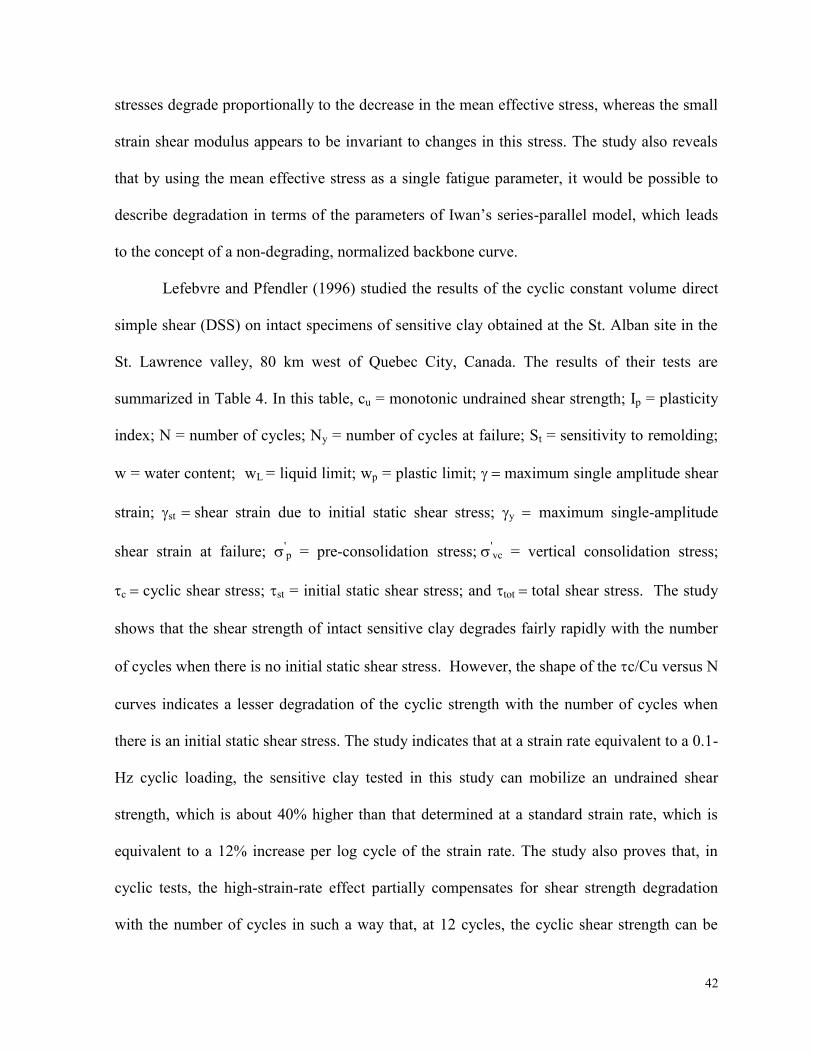
Ansal and Erken (1989) made an experimental investigation on the cyclic behavior of
normally consolidated clays by using cyclic simple shear tests on one-dimensionally and
isotropically consolidated kaolinite samples. As a result of their investigation, they developed
an empirical model to estimate the response of a soil element subjected to cyclic shear stresses
for a given number of cycles. Figure 2.7 shows the results of variation of cyclic shear stress
ratio (f)y with respect to the number of cycles, N. The linear relationship between the cyclic
shear stress ratio (f)y and the number of cycles (N) shown in Figure 2.7 is as follows:

34
1.2....................................................log Nba
yf
Where; (f)y = cyclic shear strength ratio; N = the number of cycles; and a and b = material
constants obtained from linear regression analysis. This figure also shows that, for any
specified cyclic shear strain amplitude (2%) taken as the upper allowable limit for a specific
design purpose, the same approach can be used. The results of the study also indicated that for
normally consolidated clays there is a critical shear stress ratio level or a threshold cyclic
shear stress ratio below which no pore pressure will develop, as shown in Figure 2.8. The
study also defined the variation of the slope of the pore pressure lines with respect to the
number of cycles. Figure 2.9 gives a relationship between the slope of pore water pressure
lines and the number of cycles as follows:
2.2..................................................... mRSu t
f
m = k + plog N 3.2......................................................................
Where; m = the slope of the pore pressure line u/f); N = the number of cycles; k and p =
material constants obtained from the regression analysis; and (S.R)t is the threshold cyclic
shear stress ratio. Based on their experimental study, Ansal and Erken (1989) also found that
the influence of frequency can be neglected in problems such as offshore platforms where the
number of cycles with respect to wave action will be large. The study also indicates that
cyclic behavior of normally consolidated clay, as in the case of natural deposits, is similar to
those for completely remolded clay samples. Tests show that remolded samples appear to be
more resistant to cyclic shear stresses; cyclic shear strain amplitude developed in these tests
(remolded samples) are smaller in comparison to cyclic shear strains measured in one-

35
dimensionally consolidated samples. However, the pore pressure is higher in the case of
remolded samples. Figure 2.10 and 2.11 show the comparison of the shear strain and the pore
water pressure behavior of one–dimensionally consolidated and remolded samples.
Furthermore, based on their experimental results, Ansal and Erken (1989) give a three
equation empirical model. Although the model seems to be simple and useful in predicting
shear stress ratio corresponding to a specific strain, it is based on only a simple shear test and
on only one type of one-dimensionally and isotropically consolidated kaolinite clay.
Wood (1990) analyzed the data collected by Skempton and Northey (1953) for
studying the effect of liquidity index on the undrained shear strength of sensitive clays from
various parts of the world. His study showed a clear trend of increasing sensitivity with
increasing liquidity index (IL) as shown in Figure 2.12. He used the relationship given by
Bejerrum (1954) for the Norwegian clays as follows:
4.2....................................................exp Lt kIS
Where; k is a constant describing variation in sensitivity with liquidity. A value of k~2
provides a reasonable fit. This implies a sensitivity St~7.4 for a clay approximately at its
liquid limit (w = wL, IL = 1). Based on his analysis, he established the relationship between the
liquidity index and the undrained shear strength of the sensitive clays as shown in Figure 2.13.
He assigned strengths of 2 kPa and 200 kPa for the shear strength of the soils at their liquid
and plastic limits respectively, (see Figure 2.13) and gave a relationship between the remolded
strength of the soils solely based on the liquidity index:
5.2.............................lnR)I-(kexp LRcC Lu

36
Where Cu = undrained shear strength, cL = shear strength at liquid limit, R= ratio between
shear strength at plastic limit (cP) and shear strength at liquid limit (cL), IL = liquidity index
and k = constant describing the variation in sensitivity. Furthermore, he found that, in the case
of undrained shear strength, the Mohr circle of effective stress at failure point F ( Figure 2.
14) can be associated with an infinite number of possible stress circles (T1,T2,……….)
displaced along the normal stress axis by an amount equal to the pore pressure. The pore
pressure does not affect the differences of the stresses or shear stresses, so all stress circles
must have the same size especially in case of clay soils, which are usually loaded fast to avoid
the drainage of shear-induced pore pressures.
Wood (1990) proposed that it is more desirable to mention the maximum shear stress
(f) in terms of undrained shear strength (cu), which is the radius of all the Mohr circles in
Figure 2.14. Therefore, the maximum shear stress that a clay soil can withstand and the failure
criterion for undrained conditions become:
6.2....................................................f uc
O‟ Reilly et al (1991) presented a soil model which takes into account the complexity
of stress conditions in the soil beneath structures subjected to a combination of static and
cyclic loads. Figure 2.15 shows the model‟s simplified stress conditions for some soil
elements (1, 2, 3 and 4) along a potential failure surface. In the figure, W= weight of the
platform, Hcy = horizontal shear stress, Mcy = stresses due to wind load or other cyclic
loading., DSS = direct simple shear test, = shear stress, cy = cyclic shear stress, a = average
shear stress, o = initial shear stress prior to the installation of platform and a = additional
shear stress induced by the submerged weight of the platform. The model stated that these
elements (1,2, 3 and 4) follow various stress paths which may be approximated to a triaxial or

37
a direct shear type of loading, and they are subjected to various combinations of average shear
stresses (a) and cyclic shear stresses (cy). The average shear stress (a) is composed of the
initial shear stress (o) and additional shear stress (a). The model shows that in the case of
element 2, the weight of the platform gives a higher vertical than horizontal static normal
stress hence, during cyclic loading, element 2 will tend to compress vertically. Element 4 is in
the passive zone, and the weight of the platform causes a higher horizontal than vertical static
normal stress, element 4 will, therefore, tend to compress horizontally and extend vertically
during the application of cyclic loading. Consequently, element 2 is best represented by a
triaxial compression test and element 4 by a triaxial extension test. The model also shows that
for elements 1 and 3 the shear surface will be horizontal. Therefore, these elements are best
represented by direct simple shear (DSS) tests, and these tests should be run to establish the
shear strength on the horizontal plane, i.e., the horizontal shear stress at failure. Hence, the
study emphasizes that since both the shear strength and the deformation properties of soils
under cyclic loading are anisotropic, therefore, the triaxial compression, the triaxial extension
and the DSS tests should be included in the laboratory test program for gravity structure of
some importance. It should also be noted that the model depicts the importance of the actual
conditions of stresses in the field, which are usually the combination of static and cyclic
loading.
Liang and Ma (1992) developed a constitutive model for the stress strain-pore pressure
behavior of fluid-saturated cohesive soils. The model adopts the joint invariant of the second
order stress tensor and clay fabric tensor as a formalism to account for material anisotropy.
The model includes three internal variables: the density hardening variable representing
changes in void ratio; the rotational hardening variable depicting fabric ellipsoid changes; and

38
finally, the distortional hardening variable controlling the shape of the bounding surface. The
concept of quasi-pre-consolidation pressure was used in formulating an internal variable for
the isotropic density hardening. For evolutionary laws based on micro-mechanics and
phenomenological observations, Liang and Ma (1992) constitutive model gives the
relationships for isotropic density hardening and anisotropic or rotational hardening in drained
conditions. The model considers two counterpart mechanisms for the evolution of distortional
hardening (R). One mechanism is that the bounding surface will widen along with the clay
fabric moving to preferred orientations, meaning that a smaller value of R permits lower pore
water pressure response. The other one is that the bounding surface will flatten along with the
loading involving the principal stress rotation, meaning a larger value for R causes a sharper
pore water pressure response. For un-drained conditions the model assumes that both water
and clay particles are compressible which means a zero volumetric strain. The predictive
capability of the model is tested on a database created from the available literature. The
results show that the model is quite capable of predicting the behavior of saturated clays
subjected to undrained cyclic loading, such as degradation of undrained strength and stiffness,
accumulation of permanent strain and pore pressure, influence of initial consolidation
conditions, and the effect of rotation of principal stress direction.
Wathugala and Desai (1993) modified hierarchical single surface (HiSS) models into a
modified series of models (termed as δ*) which could capture the behavior of cohesive soils.
These models consider monotonic loading as virgin loading and unloading and reloading as
non-virgin loading. An associated () model of the series was found to be sufficient for
predicting the cyclic behavior of clays. The model defines a new hardening function based on
that the normally consolidated (NC) clays that do not dilate; and instead they show a

39
contractive response under monotonic loading. The model considers the unloading phase as
elastic and reloading similar to virgin loading with some modification like a plastic modulus
for virgin loading is replaced by a plastic modulus of reloading and a unit normal tensor is
replaced by a unit normal tensor for a reference surface (R) which passes through the current
stress point in the stress space. The results show that the model is capable of capturing the
undrained shear behavior of normally consolidated clay, slightly over-consolidated clay
behavior and drained behavior during hydrostatic compression tests and stress-strain behavior
during cyclic loadings.
Hyodo et al (1993) proposed a semi-empirical model for the evaluation of developing
residual shear strain during cyclic loading. The model considers 10% peak axial strain as a
failure criterion in both reversal and non-reversal regions and gives a relationship between the
cyclic deviator stress ratio and the number of cycles required to cause failure for each initial
static deviator stress (qs). The unified cyclic shear strength is given by:
7.2.............................................κN)/pq(qRfcscycf
Where; Rf = cyclic strength ratio; qcyc = cyclic deviator stress; qs = initial deviator stress; pc =
constant mean principal stress; N = number of cycles; = 1.0+1.5qs/qc and
The peak axial strains p from all tests were related using an effective stress ratio:
.2.8........................................).........η/(2.0ηε ppp
Where; p = peak deviator stress divided by mean effective principal stress of each peak to
peak cyclic stress (qs / p). In order to introduce the undrained cyclic behavior of clay, two
parameters were introduced in the model. The first parameter defined is an index (R/Rf)
showing the possibility of cyclic failure, which is the ratio of peak cyclic deviator stress (R =
qs + qcyc) to cyclic shear strength (Rf) in a given number of cycles. R/Rf is termed as a cyclic

40
shear strength ratio and is equivalent to a reciprocal of the safety factor against cyclic failure.
When the magnitude of R is constant, R/Rf increases with the increasing number of cycles and
carries from zero at non-loading to unity at failure. The second parameter in the model is
defined as:
..2.9..............................).........η)/(ηη(ηη sfsp
*
Where; p is an effective stress ratio at the peak cyclic stress in each cycle, s is the effective
stress ratio of initially consolidated condition, f = effective stress ratio at the failure, and =
the relative effective stress ratio between initial point and final point in p-q space. These
parameters were originally introduced for sand by Hyodo et al (1991). By correlating the
values of both parameters, the model establishes a simple but useful relationship between the
accumulated peak axial strain and the effective stress ratio. The best fit curve for each relation
is given by a unique curve formulated as the following equation in spite of the difference of
initial static and subsequent cyclic deviator stresses:
.10.........2..............................}.........1)R/R-(a-/{aR/R ff *
Where; the value of “a” is given as 6.5 by the experiments of Hyodo and Suiyama (1993).
McManus and Kulhway (1993) studied the behavior of cyclic loading of drilled shafts
in laboratory-made cohesive soil (Cornell Clay). The applied loading was designed to
simulate realistic windstorm events (both one-way and two-way loading), which is an
important source of cyclic loading for foundations. Results show that for one-way uplift
loading, the upward displacement accumulated by a drilled shaft was not found to be affected
by either the size or the geometry of the model-drilled shafts or by the soil deposit stress
history. In case of two-way loading, the direction of loading reverses twice every cycle

41
causing minimal response at low load levels but a sudden degradation in displacement
response at moderate load levels, with an associated substantial reduction in capacity.
Silvestri, (1994) studied the water content relationships of sensitive clay subjected to
cycles of capillary pressures. The study presents the results of an experimental investigation
carried out to determine the volume change response of sensitive clay subjected to cycles of
air pressure in a pressure plate apparatus. Several clay samples of varying initial water content
were used in the test program. He reported that at high air pressures, the initially soft clay
specimens become less compressible than stiff clay specimens of comparable water content.
Also, the study indicates that the clay became unsaturated at a water content varying between
25 and 30%.
Bardet (1995) extended the novel concept of scaled memory (SM) model to
anisotropic behavior and presented a technique to calibrate the material constants from
laboratory data. He showed that SM generalizes closed stress-strain loops and, therefore,
avoids the artificial ratcheting predicted by bounding surface plasticity. The extended SM
model generalizes Ramberg-Osgood and Hardin Drenvich models and is simpler than, but as
capable as, multiple yield surface plasticity.
Puzrin et al (1995) showed the consistency of normalized simple shear behavior of
soft clays with the Massing rules. The study reveals that the degradation of soil properties in
undrained simple shear is considered to be the main reason for deviation of cyclic shear
behavior of soft clays from the pattern described by the Massing rules. Using the mean
effective stress as a single fatigue parameter, it was found possible to describe this
degradation in terms of Iwan‟s series-parallel model which leads to the concept of a non-
degrading, normalized backbone curve. The results of the study also prove that the set of slip
42
stresses degrade proportionally to the decrease in the mean effective stress, whereas the small
strain shear modulus appears to be invariant to changes in this stress. The study also reveals
that by using the mean effective stress as a single fatigue parameter, it would be possible to
describe degradation in terms of the parameters of Iwan‟s series-parallel model, which leads
to the concept of a non-degrading, normalized backbone curve.
Lefebvre and Pfendler (1996) studied the results of the cyclic constant volume direct
simple shear (DSS) on intact specimens of sensitive clay obtained at the St. Alban site in the
St. Lawrence valley, 80 km west of Quebec City, Canada. The results of their tests are
summarized in Table 4. In this table, cu = monotonic undrained shear strength; Ip = plasticity
index; N = number of cycles; Ny = number of cycles at failure; St = sensitivity to remolding;
w = water content; wL = liquid limit; wp = plastic limit; maximum single amplitude shear
strain; st shear strain due to initial static shear stress; ymaximum single-amplitude
shear strain at failure; 'p = pre-consolidation stress;
'vc = vertical consolidation stress;
ccyclic shear stress; st = initial static shear stress; and tottotal shear stress. The study
shows that the shear strength of intact sensitive clay degrades fairly rapidly with the number
of cycles when there is no initial static shear stress. However, the shape of the c/Cu versus N
curves indicates a lesser degradation of the cyclic strength with the number of cycles when
there is an initial static shear stress. The study indicates that at a strain rate equivalent to a 0.1-
Hz cyclic loading, the sensitive clay tested in this study can mobilize an undrained shear
strength, which is about 40% higher than that determined at a standard strain rate, which is
equivalent to a 12% increase per log cycle of the strain rate. The study also proves that, in
cyclic tests, the high-strain-rate effect partially compensates for shear strength degradation
with the number of cycles in such a way that, at 12 cycles, the cyclic shear strength can be

43
taken as equal to the undrained shear strength determined in monotonic tests at standard rates.
Thus, confirming the results of one of the previous studies using triaxial tests on sensitive clay
(Lefebvre and LeBoeuf 1987).
Yu, H. S. (1997) presented a simple, unified critical state constitutive model for both
clay and sand. The model, called CASM (Clay and Sand Model), was formulated in terms of
the state parameter, defined as the vertical distance between current state (v, p ) and the
critical state line in v-ln p space. The paper shows that the standard Cam-clay models (i.e. the
original and modified Cam-clay models) can be reformulated in terms of the state parameter.
Faker et al (1999) studied the behavior of soft clays, which usually have water content
higher than their liquid limits. The study proposes that a rotary viscometer should be used to
measure the yield stress of the super soft clays instead of using a conventional soil mechanics
apparatus. By plotting the results of yield stress measurements of soft clays in terms of w/LL,
it could be shown that the true liquid limit is 1.5 – 2 times that which is arbitrarily selected
and measured by the established conventional methods. The results of the study also show the
variation in shear stress with respect to the liquidity index (Figure 2.16). Furthermore, it is
indicated that the logarithmic of the yield stress of soft clay normalized with respect to the
equivalent effective vertical stress (σ*) on the intrinsic compression line (ICL) is linearly
related to the ratio of water content to liquid limit (w/LL) for all clays in the study, and that
the lines for each soil are parallel.
Miller et al (2000) studied the behavior of soft compacted clayey soil (used in railroad
sub-grade) subjected to repeated loading under train traffic. Cyclic triaxial tests were
conducted on tube samples at their natural water content (partially drained) and on samples
subjected to back-pressure saturation (undrained). The study indicates that, for repeatedly

44
loaded soils, a critical cyclic stress or normalized cyclic shear strength exists above which the
soil will exhibit shear failure. For the highly plastic clay tested, the normalized cyclic shear
strength was sensitive to the initial degree of saturation in the relatively narrow range
encountered, i.e., a degree of saturation (S) between 90 and 100%. For the samples at natural
water content, the normalized cyclic shear strength decreased as the initial degree of
saturation increased. An empirical relationship was defined to describe the variation of
normalized cyclic strength as a function of the degree of saturation. In the case of tests
conducted on back pressure saturated specimens or undrained conditions, the normalized
cyclic shear strength fell between 0.50 and 0.79, whereas the normalized undrained shear
strength from the static test at the same confining pressure was 0.89. The normalized
undrained cyclic shear strength for the specimen with laboratory-induced over consolidation
ratio (OCR) of 3 was greater than 0.79 for the same confining stress. The magnitude of the
deviator stresses estimated from stress cell measurements under traffic in the Low Track
Modulus (LTM) zone suggest that the cyclic shear strengths were frequently exceeded in the
nearly saturated sub-grade zones along the test track. Measurement of track settlements and
corresponding degrees of saturation appear to corroborate the relationship between cyclic
shear strength and degree of saturation.
Zhou and Gong (2001) studied soil degradation from the point of view of cyclic axial
strain through stress-controlled triaxial tests on Hangzhou normally consolidated clay.
Different influence factors on strain, such as cyclic stress ratio, overconsolidation ratio, and
frequency, were studied. Degradation index was redefined according to the tests. A
mathematical model for strain degradation was presented and verified.

45
Javed (2002) categorized the parameters that are believed to govern the behavior of
sensitive clay into two categories: physical and mechanical. The study proposed a procedure
to design and/or examine the conditions regarding foundations on sensitive clay. The study
also indicates how to use a part of Modified Cam Clay Model to cross check the reduction in
strength before and after the application of cyclic loading. A relationship is proposed for the
number of cycles, factor of safety, cyclic strength ratio with respect to sensitivity of clays.
Li and Meissner (2002) developed a two-surface model for predicting the undrained
behavior of saturated cohesive soils under cyclic loads. They used kinematic hardening and
the theory of critical state soil mechanics. The proposed model was verified with respect to
the
observed behavior of soil samples. The study shows that like other multi-surface model, this
model can realistically describe some
important responses of clays subjected to both
monotonic and cyclic loading, while incorporating the memory of particular loading events.
Oka et al (2003) proposed a cyclic viscoelastic-visco-plastic constitutive model in
order to estimate viscous effect of clay in the wide range of low to high level of strain. The
model was used to analyze the seismic response against foreshocks, main shock as well as
aftershocks of 1995 Hyogoken Nambu Earthquake. The study concludes that the proposed
model gives a good description of the damping characteristics of clay layer during large
earthquakes.
Min et al. (2004) studied, based on a series of cyclic triaxial tests, the effect of cyclic
load frequency on the undrained behavior of undisturbed marine clay. The results showed that
for a given dynamic stress ratio the accumulated pore water pressure and dynamic strain
increased with the number of cycles. The study also indicates that, a threshold value exists for
both the accumulated pore water pressure and dynamic strain, below which the effect of

46
cyclic frequency is very small, but above which the accumulated pore water pressure and
dynamic strain increase intensely with the decrease of cyclic frequency for a given number of
cycles. Furthermore, the dynamic strength increases with the increase of cyclic frequency,
whereas the effect of cyclic frequency on it gradually diminishes to zero when the number of
cycles is large enough, and the dynamic strengths at different frequencies tend to the same
limiting minimum dynamic strength. The test results demonstrate that the reasons for the
frequency effect on the undrained soil behaviors are both the creep effect induced by the
loading rate and the decrease of sample effective confining pressure caused by the
accumulated pore water pressure.
Kakoli (2004) studied the chemical aspects involved in increasing or decreasing the
shear strength of sensitive clay subjected to cyclic loading. In addition to chemical parameters
she also reviewed the effects of physical and mechanical parameters and came to the fact that
no single model can precisely predict the behavior of sensitive clay under cyclic loading.
Thammathiwat and Chim-oye (2004) studied experimentally the behavior of cyclic
strength and pore pressure characteristics of soft Bangkok clay. The experimental
investigation was conducted by using the cyclic triaxial apparatus under stress controlled and
undrained conditions. The undisturbed samples were collected at the depth of 7.50-8.00 meter
at the Faculty of Engineering, Thammasa University. The physical property test results
showed that subsoil was silty-clay with 78-95% of natural water content, LL in the range 75-
99%, PL in the range of 30-42 % and specific gravity in the range of 2.57 -2.73 . The test
results showed the axial strain and the excess pore water pressure both increased with
increasing the number of loading cycles in all cases. But the shear modulus decreased with the
increase in number of loading cycles. While, the damping ratio decreased lightly with

47
increasing the number of loading cycles. The effect of rate of loading on the cyclic properties
was also investigated. The loading frequencies adopted for the test were 0.l, 0.5 and 1.0 Hz. It
was found that the cyclic strength increased with increasing of loading frequencies for a given
confining stress but excess pore water pressure decreased with the increasing of loading
frequencies.
Vinod et al. (2005) conducted a significant number of stress-path triaxial tests with
stress probes in various directions, to study the stress-path dependent behavior of an
overconsolidated weathered crust of Champlain clay in Eastern Ontario. Both undrained and
drained tests were conducted for samples isotropically consolidated to the in situ vertical
stress and anisotropically consolidated to the in situ state of stress. The yield locus of the clay
crust was defined. The study proved that the strength-deformation and yielding behavior of
this weathered clay crust highly depends on the stress-path as well as on the in situ stress
history.
Erken and Ulker 2006 studied the effect of cyclic loads on monotonic shear strength
on torsional apparatus. Tests were conducted on both reconstituted and undisturbed fine-
grained hollow soil specimens. The existence of a critical shear strain level, called yield shear
strain, where softening starts, was determined from cyclic tests. The level of cyclic yield
strain was ± 0.75% for the reconstituted soil specimens and ± 0.5% for the undisturbed soils.
The study shows that if soil undergoes a cyclic shear strain level below the cyclic yield strain,
reduction of monotonic strength of reconstituted and undisturbed specimens is limited, but
when cyclic shear strain level is larger than yield strain monotonic strength decreases down to
40% of its initial strength.

48
Hanna and Javed (2008) defined the safe-zone, within which a combination of the
cyclic deviator stress (qcyc) and number of cycles (N) for a given soil condition, a quasi-elastic
resilient state can be achieved during the undrained period without reaching failure. The
schematic presentation of this safe zone is shown in Figure 2.17. In this figure, the failure line
should be developed in the laboratory for the given soil condition (IL, St and p). For any
number of cycles (N), the corresponding point on the failure line reveals the ultimate cyclic
deviator stress. A reasonable factor of safety should be implemented for determination of the
allowable cyclic deviator stress (qcyc), depending on the size and nature of the project. A
combination of the cyclic deviator stress (qcyc) and the number of cycles (N) located on or
above the failure line indicates that foundations built on this clay will eventually reach failure
during the undrained period.
2.1 Discussion
Studies dealing with the sensitive clays are very limited and most of them are not directly linked
with the sensitivity (St) or with the variation in sensitivity constant (k). Early investigations on
sensitive clays were focused on conducting triaxial tests on undisturbed and remolded clay for
the purpose of developing relationship between cyclic stress-strain and pore water pressure (Seed
and Chan 1966, Theirs and Seed (1968, 1969), Sangrey 1968, Sangrey et al 1969, France and
Sangrey 1977 and Sangrey et al 1978). Their study established the fact that cyclic loading
increases the pore water pressure under undrained conditions up to a number of cycles, which
defined as a critical level beyond which the failure will occur. Iwaski et al (1978) defined the
quasi-elastic resilient state of soils subjected to regular drained cycling during stress-controlled
loading between the two general stress states. Field and laboratory investigations conducted by

49
Changnon et al (1979) provide useful data base for studying the behavior of sensitive clays under
varying conditions of index properties. An interesting study reported by Houstan and Hermann
(1980) raised a question concerning the relative importance of plasticity and sensitivity and also
the need of analysis based on the combination of static and cyclic loading in the case of sensitive
clays. Matsui et al (1980) proved experimentally that an over-consolidation clay due to cyclic
stress-strain history is similar to strength to one due to the ordinary over-consolidation history.
He also established the fact that, inspite of the temporary loss in shear strength and deformation
modulus immediately after cyclic loading, the dissipation of pore pressure leads to strength
higher than the initial strength. Seed and Idris (1982) established the fact that in case of clay the
faster the rate of cycling the more the situation resembles to undrained conditions. The
experimental study of Procter and Khaffaf (1984) gives an idea that, if data from load controlled
tests are reanalyzed to account for rate effects on shear strength, then a constant value
independent of frequency is obtained. The Lefebyre and LeBoeuf (1987) experimental study on
highly sensitive clays (St>100) indicates that the effect of the strain rate on undrained shear
strength ratio appears to be the same for both naturally overconsolidated clays and normally
consolidated clays. McManus and Kulhway (1993) indicated that for a drilled shaft in a cohesive
soil foundation, a two-way moderate cyclic loading causes a sudden degradation in displacement
with an associated substantial reduction in bearing capacity. The Lefebvre and Pfendler (1996)
study shows that for a sensitive clay (St = 300) the shear strength of clay degrades fairly rapidly
with the number of cycles when there is no initial static shear stress as compared to the case
when there is an initial static shear stress component. Faker et al (1999) achieved the realistic
results by using the rotary viscometer instead of a conventional soil mechanics apparatus to
measure the shear strength of super soft clays. This approach can be used for quick clays as well.

50
Nevertheless, the results are limited to the conditions of the experimental work and do not
include the combined effect of the parameters which govern the behavior of sensitive clay
subjected to static or cyclic loading.
Eekelen and Potts (1978) introduced a fatigue parameter as a function of pore water
pressure, in the Modified Cam Clay Model, which assisted in predicting reliable results for the
shear strength of clays at the end of a given number of load cycles. Ansal and Erken (1989)
proposed an empirical model based on their experimental results and defined critical level of
cyclic deviatoric stress. Wood (1990) established a relationship among the sensitivity number,
the sensitivity constant, k (given by Bejerrum 1954) and the liquidity index. He proposed that it
is more desirable to mention maximum shear stress (f) in terms of undrained shear strength (cu),
which is the radius of all the Mohr circles. The model proposed by O‟ Reilly et al. (1991)
emphasizes that since both the shear strength and the deformation properties of soils under cyclic
loading are anisotropic; therefore, triaxial compression, triaxial extension and direct simple shear
(DSS) tests should be included in the laboratory test program for gravity structure of some
importance. Liang and Ma (1992) constitutive model's results indicate that it is quite capable of
predicting the behavior of saturated clays subjected to undrained cyclic loading, such as
degradation of undrained strength and stiffness, accumulation of permanent strain and pore
pressure, influence of initial consolidation conditions, and the effect of rotation of principal
stress direction. The Wathugala and Desai (1993) modifications for hierarchical single surface
(HiSS) model make it capable of capturing the undrained shear behavior of normally
consolidated clay, slightly over-consolidated clay, drained behavior during hydrostatic
compression tests and stress-strain behavior during cyclic loading. Hydo et al (1993) proposed a
semi-empirical model by introducing two parameters: namely, the ratio of peak cyclic deviator

51
stress to cyclic shear strength for a given number of cycles and the relative effective stress ratio
between initial and final point in p-q (deviator stress-mean effective stress) plane. Bardet (1995)
extended the Scaled Memory Model (SM) to accommodate the anisotropic behavior of the clays.
The study conducted by Puzrin et al. (1995) indicates that by using a mean effective stress as a
single fatigue parameter, it would be possible to describe degradation in cohesive soils subjected
to cyclic loading. Results of the Miller et al (2000) study confirms the studies of Sangrey et al
(1969), Matsui et al (1980) and Ansal and Erken (1989) for the critical cyclic stress level and
established an empirical relationship between cyclic shear strength ratio and the degree of
saturation. All these model studies provide useful relationship among the different governing
parameters. These models mainly deal with the normal nature of cohesive soils and extremely
useful in predicting the behavior of foundation soil when subjected to static or cyclic loading.
Nevertheless, none of the model truly addressed the complex behavior of sensitive clay. Most of
these Model studies are mainly focused on the mathematical introduction or modification of a
single physical or mechanical parameter in a proposed or an existing model to predict the
behavior of soil under a special condition. The major short coming is that none of the model can
be used as a reliable tool to design new or examine existing foundations by keeping in view the
sensitivity of the clay and the influence of the combined effect of major physical and mechanical
parameters on the complex behavior of the clay.
The schematic model for the “Safe Zone” given by Hanna and Javed (2008) was the first of
its kind to deal with this complex material and to link the physical and mechanical parameters
governing the behavior of sensitive clay. They introduced a useful guideline and theory to
predict reliable safety factor for designing foundation in those regions of clay where a wide
range of sensitivity number and extreme variations in physical and mechanical parameters exists.

52
Keeping in view the important relationships among shear stress, number of cycles,
consolidation history, pore water pressure development and strain accumulations and so forth
established by experimental investigation. The use of numerical and analytical models which
explained and further enhanced the concepts of strain hardening, normal and over-consolidation
behavior, total and effective stress paths both for static loadings and cyclic loadings.
It is therefore imperative to conduct such studies which, take into account the sensitivity of
clayey soils as a deciding element to establish a reasonable factor of safety for designing
foundations subjected to cyclic loading or combination of static and cyclic loading. The present
investigation addresses the short coming in the experimental and model investigation given in
the literature. This study redefines the useful tool of the “safe zone” (Hanna and Javed, 2008)
based on detailed experimental investigation and analysis. The study also used a well-known
existing model “Modified Cam Clay Model” to cross check the reduction in shear strength due to
cyclic load application for a given sets of governing parameters. A relationship is proposed for
the number of cycles, factor of safety, cyclic strength ratio with respect to sensitivity of clays.
Based on this discussion, the objectives of the present study can be defined as follows:
2.2 Thesis objectives
Based on literature review described above the following are the objectives of this study:
To identify and prioritize the relative importance of the governing mechanical and
physical parameters under drained and undrained conditions.

53
To model this complex behavior using the “Modified Cam Clay” to predict the shear
strength in view of various parameters, which governs this complex nature of sensitive
clay subjected to static or cyclic loading.
To establish the safe zone and to redefine its critical limits based on the selection of the
lowest shear strength ratio either from the experimental data or those predicted by using
Modified Cam Clay Model.
In order to achieve these objectives a comprehensive experimental investigation was
planned to examine the behavior of sensitive clay under the undrained or drained
conditions and subjected to static or cycling loading.
To present the result of this investigation in the form of design theory and design
procedure for practicing use.
Table 2.1: General Properties of Investigated Soils
(Lefebyre and leBoeuf 1987)
Location Depth
(m)
Natural
water
content
w (%)
Liquid
limit
wl
Plastic
limit
wp
Plasticity
Index
Ip
Liquidity
Index
Il
<
2m
Sensitiviy
St
Pre-
consoli-
dation
pressure
'p
Dyke-12 - 54-65 33.5 21.8 11.7 2.84 59 >300 112
Dyke-39 - 35-52 27 20.0 7.0 2.85 45 500 190
Olga 4 90-93 68 28 40 1.55 90 - 78
B6 6.8 50 38 24 14 1.80 76 100 145
B6 10.1 48 32.5 22.3 10.1 2.47 75.7 450 175
St. Jean - 42 36 20 16 1.38 50 100 940

54
Figure 2.1: Cyclic failure data for San Francisco Bay Mud (Houstan and Hermann, 1979)
Figure 2.2: Cyclic strength contours for San Francisco Bay Mud
(Houstan & Hermann, 1979)

55
Figure 2.3: Ratio of modified to static shear strengths versus strain rate
(Procter and Khaffaf, 1984)
Figure 2.4: Frequency response of cyclic stress ratio (cu) (Procter and Khaffaf, 1984)

56
Figure 2.5: Frequency response of modified cyclic stress ratio (c-u)
(Procter and Khaffaf, 1984)
Figure 2.6: Change of undrained strength ratio, normalized to undrained strength ratio at
strain rate for all investigated clays (Lefebyre and LeBoeuf, 1987)
Boundary

57
Figure 2.7: Cyclic yield strength versus number of cycles
(Ansal and Erken, 1989)
Figure 2.8: Cyclic stress ratio-pore pressure relationship for different numbers of cycles
(Ansal and Erken, 1989)
Number of Cycles

58
Figure 2.9: Slope of pore water pressure lines versus number of cycles
(Ansal and Erken, 1989)
Figure 2.10: Comparison of shear strain of one-dimensionally consolidated and remolded
samples (Ansal and Erken, 1989)
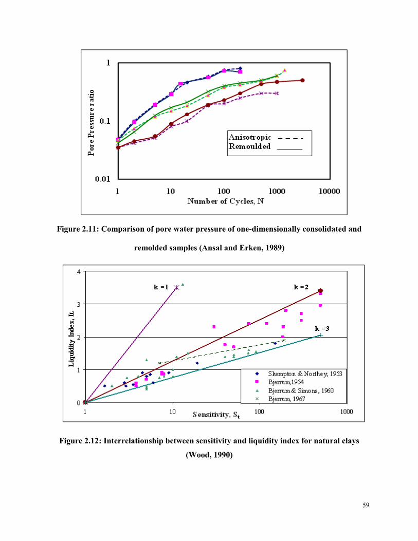
59
Figure 2.11: Comparison of pore water pressure of one-dimensionally consolidated and
remolded samples (Ansal and Erken, 1989)
Figure 2.12: Interrelationship between sensitivity and liquidity index for natural clays
(Wood, 1990)

60
Figure 2.13: variation of remolded undrained strength cu with
Liquidity index, IL (Wood, 1990)
cP = 200 kPa
cL = 2 kPa
Figure 2.14: Mohr's circles of total stress and effective stress
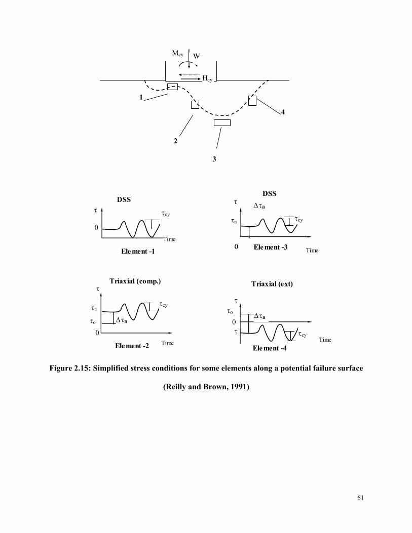
61
Figure 2.15: Simplified stress conditions for some elements along a potential failure surface
(Reilly and Brown, 1991)
Mcy W
Hcy
cy
a
o
o
a
0
0
0
0
cy
cy
a
a
a
cy
Time
Time Time
Time
Triaxial (ext)
4
3
DSS
2
Triaxial (comp.)
DSS
1
Element -1
Element -2
Element -3
Element -4
62
Figure 2.16: Variation in shear stress with respect to liquidity index (Faker et al, 1999)
)
Drained condition
Undrained condition
Number of cycles, N
Cycl
ic d
evia
tor
stre
ss, q
cy
c
Undrained/Drained
safe zone
Extended safe zone
Figure 2.17: Safe Zone for foundation on sensitive clay (Hanna and Javed, 2008

63
Chapter 3
Experimental Investigation
To achieve the goals of the present study, it was necessarily to design a well-planned
experimental framework, which is capable to answer the many outstanding questions
concerning the role of major physical and mechanical parameters affecting the shear strength
of sensitive clay under static or cyclic loading. This chapter describes the experimental set-up,
samples source, techniques used to obtain undisturbed and remolded samples, grouping of
samples, laboratory test conducted to determine the physical, mechanical, sensitivity number
and index properties and test procedure for static and triaxial compression tests.
3.1 Sample Source
Considering the nature of the sensitive clay, tests were conducted on samples that cover
reasonable variation of governing parameters. Moreover, samples are taken from sites, whose
physical and mechanical properties covering a wide range in practice. These sites are the well-
known sensitive clay regions of Eastern Canada. These sites (see Figure 3.1.1) have a well-
established database and can be considered, representative of various conditions encountered
to sensitive clay regions all over the world.
3.2 Methods of Acquiring Samples
Based on the information collected from the literature (Silvestri 1981), the block sampling
method was used to obtain undisturbed samples from different parts of Eastern Canada. The

64
samples were taken from a depth ranging 4 to 10 meters deep. A geotechnical company
named Queformat from Longueuil Quebec, has assisted in extracting these samples, where the
soil was sufficiently stiff or cemented. If however, the soil was comparatively soft,
Sherbrooke sampler was used, which give soil samples of comparable quality to that produced
by block sampling.
The block sample was obtained by cutting a column of soil about 300mm cube, so that it
would fit inside a box with a clearance of 10 to 20 mm from all sides. A box with a detachable
lid and bottom was used for storage. With the lid and bottom removed, the sides of the box
were slid over the prepared soil block, which was as yet attached to the bottom of the pit.
After filling the space between the sides of the box and block with paraffin wax, and similarly
sealing the top of the block, the lid was placed on the box. The block was then cut from the
soil using a spade, and the base of the sample trimmed and sealed. In order to obtain samples
from depth more than 3m and to avoid base heave, Sherbrooke sampler (Levebvre and Poulin,
1979) was used as shown in Figure 3.2.1.
For cylindrical samples, a borehole of about 400 mm diameter, which was best cleaned
using a flat- bottomed auger, in order to reduce disturbance and minimize the amount of
disturbed material left in the base of the hole before sampling. The hole was kept full of
bentonite mud. The sampler was lowered to the base of the hole, and rotated, using a small
electric motor, at about 5r.p.m. A cylinder of soil, about 250 mm in diameter, was carved out
by three circumferential blades, spaced at 120°. These blades made a slot of about 50mm
wide, and were fed by bentonite to help clear the cuttings. After carving out a cylinder about
350 mm high, the operator pulled a pin and the blades (which were spring-mounted) gradually
rotated under the base of the sample, as rotation was continued. Closure of the blades

65
separated the sample from the underlying soil, and the sample was then lifted to the surface
with a block and tackle. The sample was then coated with layers of paraffin wax and placed in
a container packed with damp sawdust. The disturbed samples or the samples which were
accidently disturbed used to determine most of the index properties.
3.3 Types of Selected Clays
Four types of clays with different sensitivity numbers were selected for the present research
work. To avoid any confusion, samples were identified in site for the location and depth. The
clays were named as; Type-A, Type-B, Type-C and Type-D.
The samples for the Clay Type-A were mostly taken from Petite-Patrie and Chambly
areas of Eastern, Canada. For the clay Type-B, samples were taken from Grande Balene and
St Nicolas. The samples for Type-C were taken from St. Huges and Terrebonne area. For the
clay Type-D, the samples were mostly taken from Mont. St. Hilarie area.
3.4 Grouping of Samples and Type of Tests Conducted
The clay samples obtained were divided into five groups, each group contained all types of
sensitive clays (A, B, C and D) used for the present study. Group-I consisted of virgin
undisturbed samples directly from the field. The samples of Group-II were derived from
Group-I which, were failed in triaxial static or cyclic test or got excessively disturbed while
transportation. The samples of Group-II were remolded samples, at same water contents (wc)
as Group-I. Group-III samples were derived from Groups I & II, which were failed in triaxial
static or cyclic test. The samples of Group-III were reconstituted at water content (wc) ranged
from 1 to 1.5 of LL. Therefore, Group-III represents those clay samples which, were
influenced by intrinsic aspects (intrinsic shear strength). For Groups II & III, normally
consolidated specimens were made by isotropic consolidation for 24 hours under three

66
effective confining pressures (150 kPa, 200 kPa & 250 kPa). Overconsolidated specimens
were made by isotropic consolidation under an effective confining pressure of 200 kPa,
followed by swelling for 24 hours to give an overconsolidation ratio between 1.5 and 4.
Group-IV consisted of those samples of Group-I, which reached quasi elastic resilient state at
N number of cycles in the initial cyclic triaxial test. Similarly, Group-V consisted of those
samples of Group II & III, which reached quasi elastic resilient state at N number of cycles in
the initial cyclic triaxial test. Group-IV and V samples were subjected to static undrained
triaxial test to estimate the reduction in static shear strength after suffering N number of
cycles and acquiring equilibrium state. Table 3.1 shows the grouping of these samples along
with the type of tests conducted. As a result of this grouping and sampling, various physical
and mechanical parameters were calculated and estimated, which influence in controlling the
shear strength of sensitive clays especially, when subjected to cyclic loading.
3.5 Determination of Physical and Index Properties
Physical parameters of the clay samples to include; moisture content, liquid limit, plastic
limit, degree of saturation etc. etc. were determined from the samples of Group-I or II
(disturbed samples or remolded samples). Table 3.2 presents summary of test results of the
index properties. The oven-dry- method, was used to determine the moisture content of the
soil. In brief, a mass of an empty, clean, and dry moisture-can with its lid was determined
followed by placing the moist soil in the moisture-can and securing the lid. The mass of the
moisture-can (now containing the moist soil) with the lid was then determined. Then the
moisture-can (containing the moist soil) was placed in the drying oven that was set at 105 °C

67
with its lid removed for 24 hours. After 24 hours, the moisture-can was removed cooled down
at the room temperature with its lid on the top. The new mass was determined for the moisture
can and lid (containing the dry soil). Similarly, the plastic limit was determined for the
moisture content at which the thread of soil was rolled without breaking until it was only 3
mm in diameter. For determining the liquid limit, the conventional method of counting
number of blows (droppings) to a cup containing soil sample was used. The sample was
separated by a grooving tool along a distance of 12mm until the soil sample came in contact
with the number of blows.
The samples of Clay Type-A, were taken from Petite-Patrie and Chambly, had the
water content ranged from 71% to 42 %. The average water content for the clay Type-A was
equal to 58%. The liquid limit determined for the clay Type-A ranged from 73% to 47%, and
the plastic limit from 45% to a minimum of 26%. Similarly, the plasticity index ranged from
41 to 19 and the liquidity index ranged from 1 to a minimum of 0.7. Using the plasticity chart
(Casagrande), on average the clay Type-A can be placed in the category of inorganic clays of
high plasticity. In case of clay Type-B, the maximum water content ranged from 67% to 27
%. The average water content for the clay Type-B was equal to 50%. The liquid limit
determined for the clay Type-B ranged from 70% to 24% and the plastic limit from 44% to a
minimum of 19%. Similarly, the plasticity index ranged from 33 to 5 and the liquidity index
ranges from 1.6 to a minimum of 0.6. Using the plasticity chart (Casagrande), on average the
clay Type-B can be placed in the category of inorganic clays of medium plasticity. For the
clay Type-C, the maximum water content ranged from 65% to 38 %. The average water
content for all the samples of the clay Type-C was equal to 54%. The liquid limit for the clay
Type-C ranged from 67% to 40% and the plastic limit from 29% to a minimum of 17%.
68
Similarly, the plasticity index ranged from 45 to 15 and the liquidity index ranged from 1 to a
minimum of 0.7. Using the plasticity chart (Casagrande), on average the clay Type-C can be
placed in the category of highly compressible clay with silt. For the clay Type-D, the samples
were mostly taken from Mont. St. Hilarie area of Eastern, Canada. The maximum water
content for this clay ranged from 70% to 43%. The average water content for all the samples
of clay Type-D was equal to 43%. The liquid limit for the clay Type-D ranged from 75% to
41% and the plastic limit from 31% to a minimum of 21%. Similarly, the plasticity index
ranged from 44 to 20 and the liquidity index ranged from 1.1 to a minimum of 0.9. Using the
plasticity chart (Casagrande), on average the Type-D clay can be placed in the category of
inorganic clays of high plasticity.
3.6 Conventional Consolidation Test
For this test, standard load increment duration of 24 hours was taken and at least two load
increments, including one increment after the pre-consolidation pressure. The change in
height of the sample was recorded with time intervals of approximately 0.1, 0.25, 0.5, 1, 2, 4,
8, 15 and 30 minutes; and 1, 2, 4, 8, and 24 hours. The coefficient of consolidation for each
load increment was then computed by using the following equation:
t
THc
2
v 3.1
Where; T = the dimensionless time factor (T=T50=0.197), t = time corresponding to the
particular degree of consolidation (t = t50) and, H= length of drainage path at 50%
consolidation. For the double drainage HD50 was half the specimen height at the appropriate
increment.
69
The results of these tests (in general are in accordance with ASTM standards) are
summarized in Table 3.3. For the clay Type-A the compression index (Cc) ranges from 0.541
to 0.33. The pre-consolidation pressure (p) ranges from 323 kPa to 64 kPa, and the co-
efficient of consolidation (Cv) varies from 0.068 cm2/sec to 0.015 cm
2/sec. In case of the clay
Type-B, the compression index (Cc) ranges from 0.52 to 0.144. The pre-consolidation
pressure (p) ranges from 473 kPa to 56 kPa, and the co-efficient of consolidation (Cv) varies
from 0.098 cm2/sec to 0.019 cm
2/sec. For the clay Type-C, the compression index (Cc) ranges
from 0.5 to 0.273. The pre-consolidation pressure (p) ranges from 298 kPa to 117 kPa, and
the co-efficient of consolidation (Cv) varies from 0.07 cm2/sec to 0.04 cm
2/sec. For the clay
Type-D, the compression index (Cc) ranges from 0.561 to 0.28. The pre-consolidation
pressure (p) ranges from 279 kPa to 127 kPa, and the co-efficient of consolidation (Cv) varies
from 0.08 cm2/sec to 0.013 cm
2/sec. Figure 3.6.1 shows the graph between time and
deformation in mm for one of the tests done on the samples of the clay Type-A. The pre-
consolidation stress was determined by using the Log-Time Method (due to Casagrande). A
typical e-log curve is shown in Figure 3.6.2 for the clay sample ID # 13352-GE2.
3.7 Sensitivity Number
The sensitivity as defined earlier is the ratio of undisturbed to remolded un-drained strength of
a clay soil. In order to determine the sensitivity of the tested samples the unconfined triaxial
tests were conducted on both undisturbed and remolded samples.
The remolded clay samples were prepared by using the kneading technique followed by
standard compaction. Firstly, the sample kneaded in an air tight jar for approximately 10
minutes to make sure that all the cemented bonds were broken down. Finally the sample was

70
compacted in three layers into the mould (50mm x 100mm) under a fix compacting effort
(weight of hammer = 0.25kg, drop height = 30.5 mm). A uniform remolding procedure is
adopted for all the remolded samples. Hence, the effect of remolding effort can be taken out
from the complex equation of governing parameters.
Table 3.4 shows the summary of triaxial tests conducted to determine the sensitivity
number, St. The clay Type-A bears the least sensitivity range among the four selected types.
The sensitivity number (St) for this clay ranged from 4 to 6. The clay Type-B bears, the
sensitivity number (St) ranging from 6 to 10. The clay Type-C bears the sensitivity number
(St) ranging from 10 to 14. The clay Type-D bears the sensitivity number (St) greater than 14.
Hence, the four selected types could be written as; Type-A (4≤ St ≤6), Type-B (6<St ≤10),
Type-C (10< St ≤14) and Type-D (14<St).
According to the classification given by Das (2001) in the book “Principles of
Geotechnical Engineering” fifth edition Clay A comes under the heading of medium sensitive,
Clay B as very sensitive, C as a slightly quick and D as a medium quick clay.
3.8 Triaxial Testing
Triaxial set-up was used to measure the shear strength of a soil under controlled drainage
conditions. Both, static and cyclic compression tests were conducted in order to determine the
behavior of sensitive clays under varying conditions of drainage, confining pressures,
disturbed and undisturbed states, degree of saturation etc., etc. Hence, a careful plan for
conducting these tests was prepared to handle the complexity of the experimental work.
71
3.8.1 Triaxial Test Principle and Program
In this series, a cylindrical a specimen of soil encased in a rubber membrane, was placed in
the triaxial compression chamber, subjected to a confining fluid pressure and then loaded
axially to failure. Connections at the ends of the specimen permit controlled drainage of pore
water from the specimen. Prior to the shear, the three principal stresses are equal to the
chamber fluid pressure. During the shear, the major principal stress, 1 is equal to the applied
axial stress (P/A) plus the chamber pressure, 3. The applied axial stress, 1-3 is termed the
"principal stress difference" or the "deviator stress". The intermediate principal stress, 2 and
the minor principal stress, 3 are identical in the test, and are equal to the confining or the
chamber pressure referred to as 3. Figure 3.8.1 gives a schematic sketch of this triaxial test
principle.
3.8.2 Setting up the Triaxial Apparatus for Static and Cyclic Triaxial Tests
The apparatus used in the present study is WF (Wykeham Farrance) 10056 Tritech Triaxial
Load Frame 50 kN cap. Figure 3.8.2 shows the Tritech, Triaxial load frame available at the
geotechnical lab of Concordia University. The load frame is flexible to be used as a part of
computer-controlled triaxial system or as a stand-alone unit. The frame is also equipped with
RS 232 interface, which help the triaxial setup to be connected to any computer-aided setup.
The triaxial apparatus was reassembled and calibrated properly to serve the purpose of
this research. A careful study of different components of the triaxial apparatus (Tritech 50 kN)
was done before reassembling the apparatus. Figure 3.8.3 shows the main components of the
whole triaxial testing system and the way, they were finally reassembled. The air supply
tubing and de-aired water supply, was connected to valve #1 and #2 respectively. To keep the

72
water in the air water cylinder air free, valve # 3 was connected to the base of an air bladder
assembly. The water line from valve #4, was connected to the air water cylinder. The valves
at the base of triaxial cell were connected accordingly, keeping in view, the specified valve
for the pore pressure transducer. The connectors from the four transducers were connected to
the four channels display electronic readout unit. The readout unit was further connected, to
an Agilent Data Acquisition System, which in turn, connected to the computer. This Agilent
Data Acquisition System could only communicate with other components of the triaxial
system through specific software installed on the computer. The software in turn needed a
program coded in Visual Basic (VB), to communicate among the different components of
triaxial system especially, the sample within in the triaxial cell during static or cyclic test. A
careful programming of Visual Basic was done to obtain a meaningful data output from the
triaxial tests both in the form of numbers and step by step graphical presentation to elaborate
the changes happening to the sample being tested.
3.9 Calibration of various Instruments and Transducers used in Triaxial
Testing
All testing equipment and measuring devises, to include; load cell, linear variable differential
transducers (LVDT) and pore water pressure transducers, etc were calibrated prior testing.
These calibrations were repeated often during testing to assure good results. The average
readings were taken for specific load intervals in case of load cell, lengths in case of LVDTs
and pressures for pore water pressure transducer.

73
3.9.1 Calibrating Submersible Load Cell
A 5 kN WF 17104 submersible load cell fitted with a ram was used in the current
experimental work. Before starting the triaxial test, the load cell was calibrated using a
hydraulic load applying machine in mechanical lab. The load cell was connected with a
transducer, which gave the readings in mV for the corresponding applied load. For
calibration, the load cell was loaded to its maximum capacity of 5kN with small increments of
load application by the hydraulic load applying machine. The corresponding readings in mili-
volt (mV) were noted down for the each load increment. In the similar way, the readings were
recorded during the unloading phase of the load cell. The procedure was repeated for three to
five times. The three set of reading are graphed for a load versus mV readings. A straight-line
equation is obtained and used in computer program for triaxial test. Table 3.5 and Figure 3.9.1
give the results of this calibration.
3.9.2 Calibrating LVDT
Two linear variable differential transducers (LVDT) were used, mounted to the loading
piston, external to the triaxial cell, for measuring axial displacement. For calibrating these
LVDTs metallic rings of 1.58 mm thickness were used. Both LVDT-1 and LVDT-II were
fixed in metallic frame with their suppressible needles extended to the full length in such a
way that they just touch the metallic frame base without being pressed. This was taken as zero
for calibration purposes. After that, metallic rings were inserted one by one to make the
needles deflection at equal intervals. The corresponding mV readings were noted down. These

74
readings were used to plot a linear relationship between length and milli-volt (mV) Table 3.6
and Figure 3.9.2 give the results of this calibration.
3.9.3 Calibrating Pore Pressure Transducer
The pore pressure transducer was calibrated by putting together all the assembly of triaxial
test setup, including the submersible load cell. When the system became stable, the zero for
pore pressure transducer was noted down. After that, the pressure was applied at an interval of
50 kPa till a maximum of 300 kPa. The corresponding readings in Volts were recorded as the
mili-volt (mV) was shown out of range for the pore pressure transducer. Table 3.7 and Figure
3.9.3 give the results of this calibration.
3.10 Programming the Agilent Data Acquisition System
As mentioned above, the Agilent Software works in general with the visual basic coded
program files having extension VEE. Before running the test, it was important to design an
objective oriented program, which could communicate with the sample and various
transducers before, during and at the end of a static or cyclic triaxial test. The program should
be such that it could convey the changes happening to the sample inside the triaxial cell, and
translate meaningfully these changes in form of numbers and graphical presentations. Hence,
the goal was to write a well-designed program in such a way, which could help in controlling
and displaying the output and the test results in particular fashion as required by the
researcher.
To achieve the above mentioned goal, a visual basic program named Master-Vee was
written to co-ordinate the triaxial testing system, soil sample, digital four channels display

75
electronic readout unit, Agilent Data Acquisition System and the computer. The channels
were assigned as; Channel #1 for LVDT-I, Channel # 2 for LVDT-II, Channel #3 for pore
water pressure and Channel # 4 for static or cyclic deviator stress. The straight line equations
obtained from Figures 3.9.1, 3.9.2 and 3.9.3 were used in the (Master.vee) visual basic coded
program. Master.vee gave the final output for all the channels according to their respective
units in an Excel Spreadsheet along with the graphical presentation. The program was capable
of taking readings minimum after 1 second to the maximum after one hour. Keeping in view
the nature of sensitive clay, the program was designed in such a way that an observer could
see stepwise variations in pore water pressure, stresses and strains. The gradual graphical
buildup of the stress strain curves, the pore water pressure and the stress paths with each step
recorded by the program and stored in excel spreadsheet. On top of this, one could easily
identify the stage when the stress path hit the failure envelope or if a sample attained quasi
elastic resilient state during a cyclic triaxial compression test. The subroutines of the
programs were prepared in such way that the graphical variations were adjusted automatically
to accommodate a lengthy, slow static or cyclic triaxial compression tests. The output from
the program was saved in the Microsoft Excel file named according to the sample
identification number and the type of the test run. Furthermore, a macro named Mohr‟s Circle
was designed within the “Output Excel File” to compare the shear strength values with those
determined by static triaxial compression tests. Figures 3.10.1, 3.10.2 and 3.10.3 show the
different parts of master.vee program. Figure 3.10.1 shows the overall flow chart of the
program. The Figure shows that how the different components of the program were integrated
together to make the system run according to the desired output. Figure 3.10.2 shows the
efforts involved in adjusting the programming codes. The sub-routines for Excel spreadsheet,

76
formatting codes, graphing tools and the specification of data output units were nicely
embedded in the program. Figure 3.10.3 shows the part of Excel spreadsheet for the data
output file.
3.11 Experimental Program
To achieve the goals of present study an efficient and well planned experimental framework
was important to avoid the unusual and time-consuming efforts. The experimental work along
with precautionary measures could easily nullify not all, but some of the main factors like
chemical composition and environmental impacts. Hence, many chemical and environmental
parameters could be easily balanced out from the complex equation of parameters involved in
governing the behavior of sensitive clay under static or cyclic loading. Figure 3.11.1 gives a
general layout of the experimental plan for each type of sensitive clay used in the present
study. Figure 3.11.2 shows the complexity of the experimental work in the present study. In
other words, the figure reveals the efforts involved to keep the control of various physical and
mechanical parameters which governs the behavior of the sensitive clay. This control was
maintained throughout the experimental work, in such a way, that the leading parameters
causing increase or decrease of the shear strength of the sensitive clay subjected to static or
cyclic loading could easily be identified and prioritized accordingly.
The experimental program was planned in such a way, that each type (A, B, C and D)
of soil is tested for both static and cyclic triaxial compression tests. Table 3.8 gives the details,
that how the samples from different groups (I, II, II, IV & V) were managed for this testing
plan.
77
3.12 Static Triaxial Compression Test (Undrained)
A series of isotropically consolidated undrained static triaxial compression (CU) tests were
done under different confining stresses for the clay types; A, B, C and D using 50mm
diameter by 100 mm high rubber membrane encased samples. The undisturbed samples for
Group-I were obtained from the wax coated block samples. All possible precautions while
trimming, encasing with rubber membrane, pulling over “O-rings”, placing inside the triaxial
chamber till the start of the application of deviator stress were taken to keep the sample intact
and undisturbed. Although, the samples belonging to Groups II, III, IV and V were remolded,
reconstituted or survived samples from initial triaxal testing, every possible measure was
taken to keep the integrity of those samples.
The complete list of static triaxial compression tests is given in Table 3.9. A maximum
value of 121 kPa for the clay type A (St < 6) was obtained under the undrained conditions for
a confining stress of 200 kPa, while a minimum value of 2 kPa was obtained for a remolded
sample of clay type D (St > 16) under a confining stress of 150 kPa. The strain rates of 0.5
mm/min to 1.2 mm/min were used in these static triaxial compression tests. The overall test
results show decreasing deviator stress with increase in sensitivity number (St). The samples
which were reconstituted (Group-III) at water content = LL – 1.5 LL were weaker than the
remolded samples with water content less than LL. The friction angle (‟) was determined
with the help of consolidated undrained triaxial test. For the clay Type-A the maximum
friction angle (‟) determined is about 29.75o and the minimum about 24.20
o. Similarly,
maximum friction (‟) angles are; 32o, 30.60
o, 28.21
o and minimum; 25.35
o, 21.75
o and
23.43o for the clay Types B, C and D respectively. The average friction angle (‟) value for
these clay ranges from 27o to 25
o. The values of static undrained shear strength obtained from

78
Groups IV & V gives an idea about reduction in static undrained shear strength of a sample
after suffering N number of cycles for a given level of cyclic deviator stress.
3.13 Cyclic Triaxial Compression Test
A series of 112 cyclic compression triaxial tests were conducted under varying cyclic
frequencies, drainage conditions, cyclic deviator stress and confining stress at the Concordia
University Geo-technical Laboratory. Out of these, 48 were done on undisturbed samples i.e.,
Group-I of these clays (A, B, C & D) mostly under undrained conditions. The remaining 64
tests were conducted on samples in Groups II, III, IV and V.
As mentioned above, the undisturbed samples were handled with all possible precautions
while trimming, encasing with rubber membrane, pulling over “O-rings”, placing inside the
triaxial chamber till the start of the application of cyclic deviator stress. The cell pressures,
back pressures and pore water pressures were measured by pressure transducers with a
precision of 0.25 kPa. The linear variable differential transformers (LVDT) used for axial
strain measurements, the load cells used for vertical load measurements and volume gauges
used for volume change measurements.
In case of undrained tests on back-pressure saturated specimens, water was used as the
confining pressure fluid. For unsaturated or partially saturated samples (having matric suction
component), air was used instead of water as the confining fluid to avoid the possibility of
increasing moisture content due to water penetration across the membrane. For the remolded
samples, an effective isotropic confining pressure was employed for the initial consolidation
stage, by opening the drainage valve, the specimen was consolidated isotropically in order to
allow the complete dissipation of the excessive pore-water pressures before starting the test.
For the undrained tests, the valves were closed after the test started and vice versa for the
79
drained tests. Each cyclic test was conducted under a constant cyclic deviator stress ratio right
from the beginning until the end of the test. Different cyclic deviator stress ratios (qcyc/qs =
70%, 60%, 50%, 40%, 30% and 25%) were used for the different confining stresses ranging
from 100 kPa to 250 kPa for clay types; A, B, C and D. The cyclic stress (qcyc) varied from
70% of the static deviator stress (qs) for the least sensitive clay (Type –A) under undrained /
darined contions to 20% of the static deviator stress (qs) for the remolded samples of clay
(types C and D). The Tritech Frame was allowed to increase the cyclic deviator stress till the
desired percentage of cyclic stress ratio is achieved (qcyc/qs).
To check the effect of frequency, the selected samples from Group I, II and III were
tested for frequencies ranging from 12 to 24 cycles per hour. Selection of comparatively
slower rate of load application was keeping in view that pore water pressures should allowed
to equilibrate throughout the specimen as compare to fast loading rate in which case it does
not happen. Hence, the values of pore pressure are not likely the one induced on the potential
plane of failure.
In all the tests, the deviator stress was reduced to zero or to the lower value of cyclic
deviator stress (in case of load cycle between two ranges of cyclic deviator stress) and then
reloaded to the required level of cyclic deviator stress. The cyclic tests were conducted only
on the samples belonging to Group-I, Group-II and Group-III. A summary of these cyclic
traxial test results is given in Table 3.10.
3.14 Discussion
In Group-I, samples were mostly used to get the undisturbed shear strength or maximum static
deviator strength in case of static triaxial compression tests and maximum cyclic deviator
strength in case of cyclic triaxial compression tests. Group-II samples (the failed samples of

80
Group-I) were the remolded samples at the same moisture content as their parent samples of
Group-I. Extra precautions were taken in storing these samples so they would not lose or gain
any extra moisture content other then they inherit from Group-I. Those samples were then
reconsolidated close to the initial conditions prior to testing. The final sensitivity numbers for
the clays (A, B, C & D) in the present study were obtained by the ratio of undisturbed
unconfined shear strength (Cuo) of the samples of Group-I to the corresponding unconfined
remolded shear strength of the samples of Group-II. The intrinsic shear strength (Cur*) was
obtained from Group-III reconstituted samples. These samples were reconstituted at a
moisture content (wc) equal to LL – 1.5 LL.
The first three tests shown in Table 3.8 were conducted on Group-I to check the
undrained static shear strength for the sensitive clays selected in this research. Table 3.9 gives
the results of those static triaxial tests. Based on the static shear strength the ratio for cyclic
deviator stress was decided for the cyclic triaxial tests. Tests 4 to 11 in Table 3.8 were done
on Group-I undisturbed samples for both drained and undrained conditions. The purpose for
these tests was to determine the number of cycles required by a sample of a particular clay
type and sensitivity number to get failed or reach a quasi-elastic resilient state under drained
and undrained conditions. Similarly, the tests from 12 to 17 in the Table 3.8 were done for the
remolded samples derived from Group-I but, at the same moisture content as their parent
samples under drained and undarined conditions. These tests were done at a lower cyclic
deviator stress ratio as compared to undisturbed sample tests (4-11), assuming, that a
considerable decrease in shear strength on remolding. The comparison of test results for the
disturbed and undisturbed samples gives an idea about reduction in cyclic shear strength due
to remolding. In other words the comparison gives an idea that how much the level of cyclic

81
deviator stress is needed to reduce the strength of an undisturbed sample of clay of a
particular sensitivity to its remolded shear strength for a given number cycles. In other words,
number of cycles needed to reduce the undisturbed shear strength to remolded cyclic shear
strength could be predicted. Such type of comparison could be helpful for the geotechnical
engineers to take measures for reducing the cyclic stress ratio or number of cycles especially,
in the initial stages of a construction project in the regions of sensitive clay. Similarly, the
tests from 18 to 22 were done on samples of Group-III give idea about the increase or
decrease in shear strength of sensitive clay due to matric suction (pore air pressure (ua) – (uw)
pore water pressure).
Only a few selected samples of the Group I, II and III were tested for variation in the
loading frequencies and over-consolidation ratios (OCR). Static triaxial compression Tests 23
and 24 initiate the idea of a hypothetical model that under ideal conditions the ratio of
undisturbed shear strength, Cu to disturbed or in other words remolded shear strength Cur
increases with the increase in number of cycles. Hence, a 100% undisturbed sample of
sensitive clay start displaying its sensitivity number, Cu/Cur when being disturbed by the
cyclic loading.
Overall, by carrying out the experimental work based on framework given in Tables
3.1, 3.8 and Figures 3.11.1, 3.11.2 assisted in demonstrating the behavior of sensitive clays
with different sensitivity in view of variations in physical and mechanical parameters.
Therefore, effect of reduction in static shear strength due to cyclic loading, number of loading
cycles, increase or decrease in deviator stress, frequency of cyclic loading, pre-consolidation
pressure/OCR, confining pressure, degree of saturation other parameters could easily be
analyzed keeping in view the objectives of this research. Furthermore, by adopting this

82
experimental work along with the precautionary measures helped in keeping constant most of
the chemical and environmental parameters. Hence, the experimental work has resulted in
focusing the analysis to those physical and mechanical parameters, which govern the behavior
of sensitive clay under static or cyclic loading.

83
Table 3.1 Grouping, type of sample, test conducted & parameters obtained
Group
No
Type of Sample
Type of Tests
Conducted
Parameters determined
Groups I
& II
Disturbed or
remolded Atterberg Limits LL, PL, IP, IL & Activity
Group -I Undisturbed
Static Odeometer
Compression Test or
Consolidation Test
Virgin comp. index (Ic),
recomp. index (Ir) co-
efficient of consld. (cv)&
preconsld. stress (p)
Group -I Undisturbed Static Triaxial
Compression Test
Axial Strain (), Pore water
pressure (u) & Static shear
stress (f)
Group -I Undisiturbed Cyclic Triaxial
Compression Test
Axial Strain (), Pore water
pressure (u), cyclic shear
stress (c) & Number of
cycles (N)
Group-II
Remolded at same
water content as
Group-I
Static Odeometer
Compression Test or
Consolidation Test
Virgin comp. index (Ic),
recomp. index (Ir) co-
efficient of consld. (cv)&
preconsld. stress (p)
Group-II
Remolded at same
water content as
Group-I
Cyclic and Static
Triaxial Compression
Test
Axial Strain (), Pore water
pressure (u), cyclic shear
stress (c) & Number of
cycles (N)
Group -III
Reconstituted at w
=LL-1.5LL
(Intrinsic Shear
Strength)
Static Odeometer
Compression Test or
Consolidation Test
Virgin comp. index (Ic),
recomp. index (Ir) co-
efficient of consld. (cv)&
preconsld. stress (p)

84
Table 3.1(continued): Grouping, type of sample, test conducted & parameters obtained
Group-III
Reconstituted at w
=LL-1.5LL
(Intrinsic Shear
Strength)
Cyclic and Static
Triaxial Compression
Test
Intrinsic axial strain (),
Pore pressure (u) & Intrinsic
Static (INT) and cyclic shear
stress (cINT)
Group -IV
Group-I Samples
reached Quasi
Elastic State
Static Compression
Test
Axial Strain (), Pore
pressure (u) & Reduction in
static strength after N no. of
cycles
Group -V
Group-II Samples
reached Quasi
Elastic State
Static Compression
Test
Axial Strain (), Pore
pressure (u) & Reduction in
static strength after N no. of
cycles

85
Table 3.2: Summary of index property test results
Clay Type Depth m w.c (%) LL (%) PL (%) IL IP Location
A
Avge. 7 57.8 60.8 31.4 0.9 29 Petite-Patrie,
& Chambly Max. 10 71 73 45 1 41
Min. 4 42 47 26 0.7 19
B
Avge. 7 49.8 53.3 28.9 0.9 24 Grande Balene
& St Nicolas
Max. 10 67 70 44.8 1.6 33
Min. 4 27 24 19 0.6 5
C
Avge. 7 54.7 57.9 25.7 0.9 32
St Huges
& Terrebonne Max. 10 65 67 29 1 45
Min. 4 38 40 17 0.7 15
D
Avge. 7 60.5 62.4 27.8 1 35
Mont. St Hilarie Max. 10 70 75 31 1.1 44
Min. 4 43 41 21 0.9 20
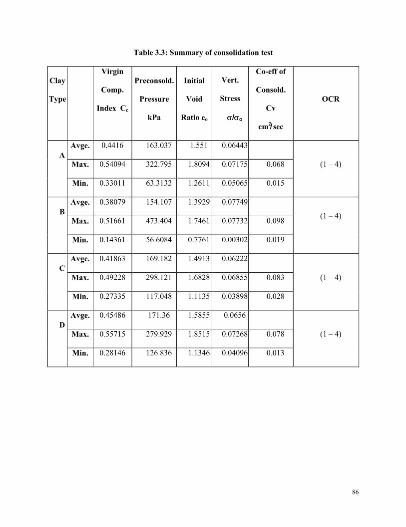
86
Table 3.3: Summary of consolidation test
Clay
Type
Virgin
Comp.
Index Cc
Preconsold.
Pressure
kPa
Initial
Void
Ratio eo
Vert.
Stress
/o
Co-eff of
Consold.
Cv
cm2 sec
OCR
A
Avge. 0.4416 163.037 1.551 0.06443
(1 – 4) Max. 0.54094 322.795 1.8094 0.07175 0.068
Min. 0.33011 63.3132 1.2611 0.05065 0.015
B
Avge. 0.38079 154.107 1.3929 0.07749
(1 – 4)
Max. 0.51661 473.404 1.7461 0.07732 0.098
Min. 0.14361 56.6084 0.7761 0.00302 0.019
C
Avge. 0.41863 169.182 1.4913 0.06222
(1 – 4) Max. 0.49228 298.121 1.6828 0.06855 0.083
Min. 0.27335 117.048 1.1135 0.03898 0.028
D
Avge. 0.45486 171.36 1.5855 0.0656
(1 – 4) Max. 0.55715 279.929 1.8515 0.07268 0.078
Min. 0.28146 126.836 1.1346 0.04096 0.013
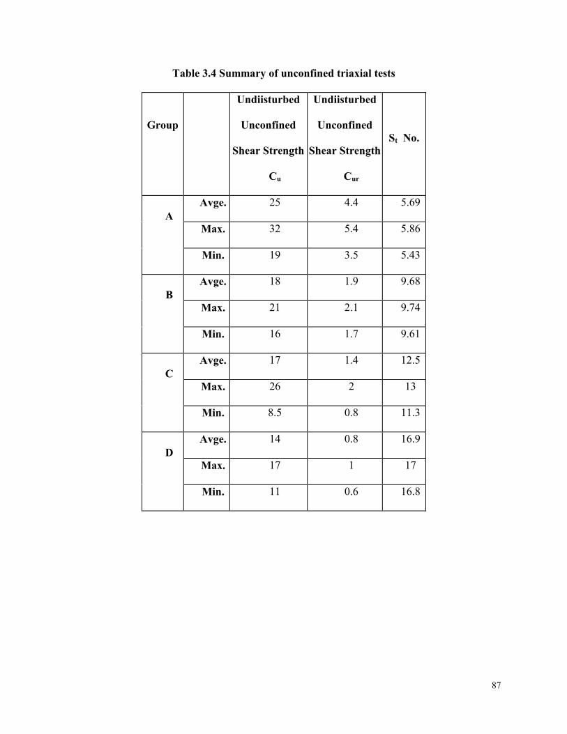
87
Table 3.4 Summary of unconfined triaxial tests
Group
Undiisturbed
Unconfined
Shear Strength
Cu
Undiisturbed
Unconfined
Shear Strength
Cur
St No.
A
Avge. 25 4.4 5.69
Max. 32 5.4 5.86
Min. 19 3.5 5.43
B
Avge. 18 1.9 9.68
Max. 21 2.1 9.74
Min. 16 1.7 9.61
C
Avge. 17 1.4 12.5
Max. 26 2 13
Min. 8.5 0.8 11.3
D
Avge. 14 0.8 16.9
Max. 17 1 17
Min. 11 0.6 16.8

88
Table 3.5: Calibration of submersible load cell 5 kN
Table 3.6 Calibration for LVDTs
S.No Volts Observed m-Volts Observed m-Volts
mm Readings mm Readings
LVDT-I LVDT-II
1 1.58 2.345 1.57 255.64
2 3.16 5.964 3.14 265.53
3 4.74 9.86 4.71 273.46
4 6.32 13.51 6.28 281.62
5 7.90 17.387 7.85 287.63
6 9.48 21.145 - -
7 11.06 24.849 - -
S. No. kN loading unloading loading unloading loading unloading Readings
1 1 2 2 3 3 Average
1 0.56 0.0069 0.0071 0.0072 0.0074 0.0070 0.0073 0.0072
2 1.13 0.0308 0.0310 0.0308 0.0309 0.0310 0.0310 0.0309
3 2.15 0.0740 0.0743 0.0739 0.0741 0.0740 0.0742 0.0741
4 3.50 0.1259 0.1261 0.1258 0.1260 0.1258 0.1260 0.1259
5 3.88 0.1389 0.1391 0.1390 0.1392 0.1390 0.1391 0.1391
6 5.00 0.1828 0.1829 0.1827 0.1830 0.1828 0.1829 0.1829

89
Table 3.7: Calibration for pore water pressure transducer
S.No Volts Observed m-Volts
Readings kPa Readings
1 0.054 75.00 54
2 0.07626 100.00 76.26
3 0.12255 150.00 122.55
4 0.165 200.00 165
5 0.186 225.00 186
6 0.20965 250.00 209.65
7 0.231 275.00 231
8 0.252 300.00 252
9 0.2733 325.00 273.3
10 0.295 350.00 295
11 0.301 360.00 301

90
Table 3.8 Nature of tests conducted on each type of sensitive clay (A, B, C and D)
Test
No.
Grp
No.
Pre-con.
Lab /
Field
OCR Drainage
Condition
No. of
Cycles
Freq.
fz
cyc/h
Confining.
Pressure
(kPa)
Cycic deviator
Stress
(qcyc)(kPa)
1 I L a b 1 Undrn.
Static -
≥p
2 I I L a b 1 Undrn.
Static
- ≥p
3 I I I L a b 1 Undrn.
Static
- ≥p
4 I L a b 1-4 Undrained N 12-24 /hr ≥p 70- 60% qs
5 I L a b 1-4 Undrained N 12-24 /hr ≥p 6 0 -5 0 % q s
6 I L a b 1-4 Undrained N 12-24 /hr ≥p 5 0 -4 0 % q s
7 I L a b 1-4 Undrained N 12-24 /hr ≥p 4 0 -3 0 % q s
8 I L a b 1-4 Drained N 12-24 /hr ≥p 70- 60% qs
9 I L a b 1-4 Drained N 12-24 /hr ≥p 6 0 -5 0 % q s
1 0 I L a b 1-4 Drained N 12-24 /hr ≥p 5 0 -4 0 % q s
1 1 I L a b 1-4 Drained N 12-24 /hr ≥p 4 0 -3 0 % q s
1 2 I I L a b 1-4 Undrained N 12-24 /hr ≥p 5 0 -4 0 % q s
1 3 I I L a b 1-4 Undrained N 12-24 /hr ≥p 4 0 -3 0 % q s
1 4 I I L a b 1-4 Undrained N 12-24 /hr ≥p 3 0 -2 0 % q s
1 5 I I L a b 1-4 Drained N 12-24 /hr ≥p 6 0 -5 0 % q s
1 6 I I L a b 1-4 Drained N 12-24 /hr ≥p 5 0 -4 0 % q s
1 7 I I L a b 1-4 Drained N 12-24 /hr ≥p 4 0 -3 0 % q s
1 8 I I I L a b 1-4 Undrained N 12-24 /hr ≥p 3 0 % q s
1 9 I I I L a b 1-4 Undrained N 12-24 /hr ≥p 2 5 % q s
2 0 I I I L a b 1-4 Undrained N 12-24 /hr ≥p 2 0 % q s
2 1 I I I L a b 1-4 Drained N 12-24 /hr ≥p 3 0 % q s
2 2 I I I L a b 1-4 Drained N 12-24 /hr ≥p 2 0 % q s
2 3 I V L a b 1-4 Static
Comp.
- -
≥p 6 0 % q s
2 4 V L a b 1-4 Static
Comp.
- -
≥p 4 5 % q s

91
Table 3.9 Summary of static triaxial compression test
3, kPa
1 -
3 kPa
u
Pm
m/m
in
1Drained_Static_S-13252_GE-2 FO
S- TS06 4.80-4.9S-13252_GE
20080
checkcheck
checkA
Grande-Baleine4 - 6
2Rem
-Static_13293-G(2) BH-02 - TS-04_3.5-3.613293-G(2)
150n/a
n/an/a
n/aA
Alexandria, Ont
4 - 6
3Static_13227_E- FO
I-TS-09_ 11.0-11.1013227_E- F
15047
9011%
1.2A
Saint-Hugues4 - 6
4Static_13293-G(2) BH-02 - TS-04_3.5-3.6
13293-G(2)150
6062
11%1.2
AAlexandria, O
nt4 - 6
5Static_13293-G_3.5-3.60
13293-G_3.200
58101
19%1.2
AAlexandria, O
nt4 - 6
6Static_13293-G_BH-02_TS-04_3.5-3.6
13293-G_BH200
60112
18%1.2
AAlexandria, O
nt4 - 6
7Static_13352_GE2 FO
2.TS-09 5.05-5.15 A13352_GE2
30063
30310%
1.2A
Petite-Patrie, QC
4 - 6
8Static_13352_GE2 FO
2.TS-09 10.30-10.40 D13352_GE2
200121.3
1099%
1.2A
Petite-Patrie, QC
4 - 6
9Static_13352_GE2- FO
I-TS-05_ 4.60-4.7013352_GE2-
15051
976%
1.2A
Petite-Patrie, QC
4 - 6
10Static_13352_GE F10.TS-05 4.20-4.30 D
13352_GE F200
38185
9%1.2
APetite-Patrie, Q
C4 - 6
11Static_S12647-11G_FO
ITSS_12.4-12.5S12647-11G
20045
1606%
1.2A
Grande-Baleine4 - 6
12Static_S-13252_ZFI- PO
-301-E 0.5-0.6S-13252_ZF
20048
15811%
1.2A
Grande-Baleine4 - 6
13Rem
-Static_S-13252_ZFI- PO-301-E 0.25-0.5A
S-13252_ZF100
32check
checkcheck
BGrande-Baleine
6 - 10
14Rem
-Static_13221-G_FOITS-08_4.50-4.60
13221-G_FO150
18126
19%1.2
BSt-N
icolas6 - 10
15Static_13221-G_FO
ITS-08_4.50-4.6013221-G_FO
25027
576%
0.5B
St-Nicolas
6 - 10
16Rem
-Static_13352_GE2 FO2.TS-09 10.30-10.40 D
13352_GE2 150
13169
20%0.2 / 0.5
CPetite-Patrie, Q
C10-14
17Rem
-Static_S-13252_GE-2 FOS- TS06 4.80-4.9
S-13252_GE150
1293
19%1.2 / 5.2
CGrande-Baleine
10-14
18Rem
-Static_13352_GE- F10-TS-05_ 3.90-4.00A13352_GE-
10010
3620%
1.2C
Petite-Patrie, QC
10-14
19Static_13252_ZN
A- DO-301.E-0.25-0.35A
13252_ZNA-
20031
1266%
1.2C
Grande-Baleine10-14
20Static_13252_ZN
A- PO-301.E-035-0.45
13252_ZNA-
25029
21010%
1.2C
Grande-Baleine10-14
21Static_13252_ZN
A- PO-301.F-3.50-3.60
13252_ZNA-
20026
2012%
1.2C
Grande-Baleine10-14
22Static_S13048-G_BH-02_10.80-10.90
S13048-G_B200
40.35150
14%1.2
CTerrebonne, Q
C10-14
23Static_S13048-G_BH-02_13.70-13.80
S13048-G_BC
Terrebonne, QC
10-14
24Static_S12647-11G_FO
ITSS_11.5-11.6S12647-11G
15052
6211%
1.2C
Mont St-Hilarie, Q
C10-14
25Static_S-13252_CLT PO
-301.G-0.2-0.3S-13252_CL
20017
18510%
1.2C
Grande-Baleine10-14
26Rem
-Static_13252_CLT PO-301.J-0.2-0.35
13252_CLT 200
6188
12%1.2
DGrande-Baleine
> 14
27Rem
-Static_13252_CLT PO-301.J-0.35-0.55
13252_CLT 150
2106
20%0.5
DGrande-Baleine
> 14
Clay TypeN
ame of the site
Sensitivity
rangeS. N
o.N
ame of the O
ut Put FileSam
ple ID
No.
Confining
Pressure
kPa
Static
Dev.
Stress
Peak
Pore
Pressure
Peak
Axial
strain
Strain
Rate

92
Table 3.10 Summary of cyclic triaxial compression test

93
Table 3.10 (continued): Summary of cyclic triaxial compression test

94
Table 3.10 (continued): Summary of cyclic triaxial compression test
Nam
e of the Output File
Test IDConfining Static D
ev.G
roupPore Pres.
P (%
) atCyclic D
ev.%
Test N
umber
/ Nature of Test
pressureStress
No.
u (takn)taken
Stressqcyc/qs
ResultCycles, N
Rem-Cyclic_13352_G
E2 FO2.
C95
15015
II132.7554
1.05%4.5
30%equilibrm
105
Rem-Cyclic_13252_ZN
A- PO
-C
96150
12II
126.79540.83%
325%
equilibrm117
Rem-Cyclic_13252_ZN
A- PO
-C
97150
12II
127.85540.83%
2.420%
equilibrm125
Rem-Cyclic_S13048-G
_BH-02
C98
15012
II125.7754
0.83%4
33%equilibrm
113
Rem-Cyclic_13252_ZN
A- PO
-C
99150
12II
120.77540.83%
433%
equilibrm109
Rem-Cyclic_13252_ZN
A- PO
-C
100150
12II
116.77540.83%
325%
equilibrm129
Rem-Cyclic_S13048-G
_BH-02
C101
15012
II131.7754
0.83%4
33%equilibrm
116
Rem-Cyclic_13352_G
E2 FO2.
C102
20015
II163.5172
0.78%4.5
30%equilibrm
122
Rem-D
rained_Cyclic_S13048C
103150
10III
112.77540.69%
330%
equilibrm126
Rem-Cyclic_13252_ZN
A- PO
-C
104150
12II
131.42540.83%
433%
equilibrm115
Rem-Cyclic_13252_ZN
A- PO
-C
105150
12II
126.20540.83%
433%
equilibrm121
Cyclic_13252_CLT PO-301.J
D106
20067
I175.6972
4.14%20
30%equilibrm
76
Cyclic_13252_CLT PO-301.J
D107
20067
I190.3672
4.02%17
25%equilibrm
98
Cyclic_13252_CLT PO-301.J
D108
20067
I190.3672
4.02%13.5
20%equilibrm
86
Rem-Cyclic_13252_CLT PO
-3D
109200
12III
190.36720.62%
3.630%
equilibrm87
Rem-Cyclic_S12647-11G
_FOI
D110
2007
II190.3672
0.36%2.45
35%equilibrm
67
Rem-Cyclic_S12647-11G
_FOI
D111
1507
II142.7754
0.48%2.3
33%equilibrm
84
Rem-Cyclic_S12647-11G
_FOI
D112
1007
II95.18361
0.73%2.1
30%equilibrm
93

95
Figure 3.1.1: Region of sensitive clay from where the samples are taken for the present
study River Lowlands (Loacat, J., 1995)
Figure 3.2.1: Schematic diagram of the Sherbrooke down-hole block sampler
(Lefebvre and Poulin 1979).

96
Figure 3.6.1: Consolidation Test–Deformation (mm) versus Time (min) Clay Type-A
Figure 3.6.2: Typical consolidation curve (e-log v) for sample 13352-GE2

97
Figure 3.8.1: Schematic sketch of triaxial test principle
Figure 3.8.2:- Tritech, Triaxial Load Frame at Concordia University Geotechnical
Laboratory
Deviator stress = σ 1 - σ 3
Prior to shear, σ 1 = σ 2 = σ 3 = σ c
During shear, σ 1 = P/A + σ3
σ 2 = σ 3 throughout the test
Valve #1
Valve #2
Valve #3
Valve #4

98
Figure 3.8.3: Main Components of the Triaxial System and the way they are connected.
Figure 3.9.1:- Calibration – Submersible Load Cell 5 kN

99
Figure 3.9.2: Calibration Curve for LVDT
Figure 3.9.3: Calibration Curve for Pore Water Pressure Transducer

100
Figure 3.10.1 Overall Master.vee Visual Basic based program
Includes EXCEL File output Subroutine

101
Figure 3.10.2 Overall Master.vee Visual Basic Coded Program – Showing Program Codes

102
Figure 3.10.3: Master.vee - subroutine for setting up Excel Worksheet for data output
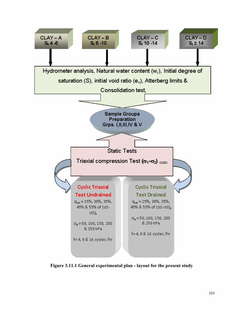
103
Figure 3.11.1 General experimental plan - layout for the present study

104
Figure 3.11.2:- Complexity of the experimental work
Clay_A (St= 4-6)
Clay_B (St =6-
10)
Clay_C (St =10-
14)
Clay_A (St > 1
4)
Clay Type

105
Chapter 4
Analysis and Theory
This chapter deals with the detailed analysis of the experimental results especially, static and
cyclic triaxial tests. The purpose is to analyze the behavior of sensitive clay and to indicate the
important factors and the missing gaps for the experimental and model investigation mentioned
in the literature. Also, to formulate such a strategy which is capable of addressing also those
missing gaps and provide the practical solutions to geotechnical engineers dealing with the
complexity of designing new or examining existing foundations on sensitive clay.
The key elements responsible for the complex behavior of sensitive clay are identified
and prioritized especially, when subjected to cyclic loading. Since, experimental work took care
of the chemical and environmental parameters therefore the analysis is focused to those physical
and mechanical parameters, which govern the behavior of sensitive clay when subjected to static
or cyclic loading. Physical parameters include; natural water content (w), liquid limit (LL),
plastic limit (PL), plasticity index (IP), liquidity index (IL), sensitivity (St), constant of variation
in sensitivity (k) and initial degree of saturation (S). Whereas, mechanical parameters include;
cyclic deviator stress (qcyc), pore water pressure (u), axial strain (), over consolidation ratio
(OCR), preconsolidation pressure (p), confining pressure (3), and number of cycles (N). In the
graphical analysis to show the effect of mechanical parameters the number cyclic loading (N) is
taken as abscissa i.e., along X-axis and the other parameters along Y-axis. Number of cycles, N
helps in indicating cycle by cycle effect of other mechanical parameters. The analysis assisted in
identifying those parameters which establish the link between the two governing categories of
parameters i.e. physical and mechanical.

106
A hypothetical model, which explains the behavior of sensitive clay and how its shear strength
reduces when subjected to disturbing /remolding action of cyclic loading has been introduced.
The hypothetical model is used to adapt the Modified Cam Clay Model for predicting shear
strength of sensitive clay subjected to cyclic loading under varying field conditions. The most
important of all that the analysis and theory assisted in redefining the safe zone limits, which
covers all the shortcomings in the study of Hanna and Javed, 2008. The redefined “safe zone”
along with theoretical guide line is a tool, capable of addressing most of those missing gaps
mentioned in literature and provides the practical solution to geotechnical engineers dealing with
the complexity of designing new or examining existing foundations on sensitive clay.
4.1 Static Triaxial Tests
Conventional static triaxial compression tests were conducted on the selected clay samples.
Figures 4.1.1 – 4.1.4 show the plotted data for stress versus peak axial strain and pore water
pressure versus peak axial strain. Figure 4.1.5 and 4.1.6 show the typical stress-strain and pore
water pressure versus strain curves for some of the selected samples
From the Figures 4.1.1 – 4.1.4 it is clear that strains at the peak shear stress for the most
the samples were in the range of 0.3% to 3%, which is consistent as far as the of these clays, are
concerned. These figures also show that, the samples from shallow depths have higher axial
strain at failure as compared to those from greater depths. The possible reasons for this could be
that, the samples at greater depths were more cemented and brittle than those taken from shallow
depths. Also, the other possible reason might be that the samples taken from upper soil were
loose and having random crack of microscopic proportion, hence, produced less pronounced
peak stress requiring higher strain for failure.

107
The typical curves shown in Figures 4.1.5 and 4.1.6 also pin point an interesting fact that
the sample at shallow depths behaved more or less like over consolidated clays (OCC) while,
those at higher depths like normally consolidated clays (NCC). The obvious peaks in stress strain
curves for test ID 6 A-I, sample ID S-13293-G BH and test ID 15 B-I, sample ID 13221 taken
from depth 3.5m as compared to normally consolidated samples test ID 21 C-II, sample ID
13253 ZNA and test ID 2 A-III, sample ID 13293-G(2) further supports this fact.
The peak static strength shown in Figures 4.1.1 and 4.1.2 indicate that the samples
belonging to Group-I were stronger than those of group II and III. The graphical analysis shows
that the shear strengths for undisturbed samples were higher than remolded or reconstituted
samples of groups II and III. There could be a number of reasons for this; as mentioned in the
introduction about the card house structure of sensitive clays, the undisturbed samples initially
show a high strength at lower strains and then in most of the cases a sudden drop occurred as the
card house collapsed. Usually, when an undisturbed sample is brought to the laboratory, in spite
of best efforts, somehow the sample loses or gains moisture content in addition to degree of
disturbances a sample suffered in transporting process. These factors make the sensitive clay
sample more unpredictable as compared to other non- sensitive or less sensitive clays. The most
delicate part is keeping an undisturbed sample 100% free form addition or subtraction of
moisture content. The samples of Group III whose natural water content was already close to
liquid limit behave as a sample of soil bearing intrinsic shear strength. On the other hand, loss in
moisture content while remolding and compacting could lead to the development of matric
suction showing higher strength as a partially saturated sample. The Test 25C-I of Group-I has
almost the same shear strength as of and 16C-III of Group –III. The possible reason for this gain
of strength is due to the loss of moisture content during remolding. In general the Group-III
108
samples have least shear strength among the three groups. The other possible reason that test
25C-I is done on a sample obtained from shallow depth, which was already at the border line of
partially saturation. Hence, the sample became brittle and end up in failure in the very early
stages of the test.
Similarly by comparing Groups II and III (Figures 4.1.1 - 4.1.6), it is clear that effect of
increased moisture content in the reconstituted (water content equal or greater than liquid limit)
had made those samples weaker than the remolded samples for the same clay type belonging to
Group II, for the same deviator stress and confining pressure combinations. The same trend can
be observed in pore water pressures (see figures 4.1.3, 4.1.4 & 4.1.6). The Group III samples
produced higher pore water pressures as compared to Group-II for the same or close match of
deviator stress and confining pressure combinations. Hence, the samples bearing the intrinsic
shear strength (Group-III) represents the critical level of deviator stress for the sensitive clay.
Static triaxial tests done for group IV (samples attaining equilibrium in Group-I cyclic
triaxial test and V (samples attaining equilibrium in Group-II cyclic Triaxial test) are shown in
Figures 4.12.3 and 4.12.4. The analysis Results for those test where also amazing, like; 1)
Obvious reduction in static strength due to disturbance caused by initial cyclic test. 2). Over-
consolidated samples behave like normally consolidated samples when subjected to same or
higher deviator stress as was in cyclic test. The possible reason might be that after suffering N
no. of cycles, samples stress history was changed so it behaved like a NCC sample 3). Also, an
interesting fact was revealed that the sensitivity number reduces for the same soil type with an
increase in sample taking depth. In other words, same soil showing different sensitivity number
is dependent on the stress history and number of vibration which that layer of soil suffered before
the sample was taken. This fact is supported by the results of static triaxial tests on the samples

109
of Group IV and V which, attained equilibrium or quasi elastic resilient state without being failed
in the initial cyclic triaxial tests.
4.2 Cyclic Triaxial Tests
Only a few tests were done as consolidated undrained (CU), mostly unconsolidated undrained
(UU) triaxial compression tests were done in view of variations in both physical and mechanical
categories of parameters. A summary of cyclic triaxial test results is given in Figures 4.2.1 –
4.2.4. Figures 4.2.5 – 4.2.10 (Test ID A57 / Sample ID S-13252_ZF) show the typical stress
versus time, pore water pressure versus time, stress versus strain and pore pressure versus strain
patterns in cyclic tests. It is clear from the figures that both the pore water pressure and the axial
strains increase with the increase in the number of applications deviator stress. The increase in
pore pressure is the cause of stress path movement towards the static failure envelope (Figure
4.2.10). The samples which attained quasi elastic resilient state at the end of cyclic test without
failing have cyclic strains less than 5%. Test ID – D110, Group II sample ID S-12647-11G
attained quasi elastic resilient state at a minimum strain of 0.36%. Test ID – A62, Group III
sample ID S-13213-G_PE attained quasi elastic resilient state at a maximum strain value among
the survived samples of 6.5%. The maximum value of the cyclic deviator stress under which any
sample survived was 55% for drained test, Test ID – A55, Group II, sample ID S-13252_ZF
belonging to clay Type-A. On the other hand four samples with IDs A62, A65, C97 & D108,
Groups III, II, II & I, sample IDs 13213-G_PE, 13293-G_BH, 13252_ZNA & 13252_CLT
respectively got equilibrium at a minimum cyclic deviator stress ratio of 20%. Samples from
shallow depths showed less pore water pressure values for approximately same strains as
compared to the reconstituted samples of Groups II & III or those obtained from greater depths.
The possible reason for this is again the OCR trend of shallow samples like the case of static
110
tests. The overall scenario shown in Figures 4.2.1 – 4.2.4 tells that there are many parameters in
the back ground which could not be shown in these figures played decisive role in the survival or
failure of the samples being tested. In some cases, apparently weaker samples (having higher
sensitivity number) survived at same deviator stress at which the stronger samples (low
sensitivity number) could not able to stand. For instance, Test ID – C33, Group II, sample ID S-
13352_GE2 failed at cyclic deviator stress ratio of 35%, while sample test ID – D110, Group II,
sample ID S12647-11G survived. A careful review shows that under certain conditions confining
pressure was the decisive parameter. Sample of clay Type-C almost under same conditions as of
sample of Clay Type-D, the only difference was that Type-C tested under a confining pressure
of 100 kPa, while the sample for clay Type-D was tested under a confining stress of 200 kPa.
Similarly in many tests where the sample was inclined towards overconsolidation a decrease in
pore pressure in the initial loading cycles delay the migration of stress path towards failure.
Similarly, application of low cyclic stress level could result in dilation and negligible stress
conditions for the tested samples. Hence, many factors like; confining stress, deviator stress
ratio, in situ stress states, disturbed/undisturbed or structured/ de-structured state of samples
number and frequency of load applications, water content, degree of saturation, sensitivity
number etc., etc., become responsible directly or indirectly in attaining equilibrium or failure for
the clay samples tested for a triaxial compression test. Under certain conditions as mentioned in
above example of clay, Types C & D a single parameter becomes dominant and play the decisive
role.
The awareness of the complexity in the behavior of sensitive clay created by the current
section demands a clear identification and prioritization of the role of all those physical and
mechanical parameters which govern the behavior of sensitive clay under cyclic loading.

111
Keeping in view the importance of these parameters, the succeeding sections of the present
chapter analyzes one by one the situations under which these parameters take over the control of
the behavior of sensitive clay and become reason for attaining equilibrium or failure for the
samples tested in triaxial compression tests.
4.3 Drained and Undrained Triaxial Compression Tests
Three drained tests were carried out on the selected samples of clay Types A and C. The purpose
of these tests was to clarify the fact that the drained cyclic shear strength of a clay sample is
always greater than undrained shear strength for a given stress condition. In triaxial testing,
especially for clays due to poor hydraulic conductivity, to obtain 100% drained sample need
more time requiring and ideally impossible. Hence, the drained strength is estimated with the
help of undrained triaxial tests. In case of undrained triaxial test, the undrained shear strength
behavior of sensitive clay differs significantly if test at in-situ stresses, or if test at stresses higher
than the preconsolidation pressure (p). Chapter 3, Figure 3.6.2 is based on the conventional
consolidation test results. Although a significant part of the curve is under normally consolidated
region, but the importance of over consolidated region cannot be overlooked, which usually
causes a negative pore water pressure. The effective stress which governs the undrained shear
strength in a sensitive clay foundation is a vertical effective stress in the soil at the time of
construction, and the highest vertical stress previously experienced by the soil. The lowest
undrained shear strength occurs when the current vertical effective stress equals the previous
maximum value, which is a state of normally consolidated clay. Hence, the triaxial undrained
tests done on samples having OCR close to 1, give critical values for shear strength as compared
to the drained shear strength values obtained from drained cyclic triaxial test. Figure 4.3.1 shows
stress strain chart for drained and undrained triaxial compression tests done on clay Type-C.
112
Drained tests exhibited shear failure at a higher deviator stress with an accumulated strain range
of 6.23% - 6.71%, while, survived samples‟ accumulated strain range is 1.44% - 2.88%, at
comparatively low cyclic deviator stress. On the other hand, undrained tests showed large
accumulated strains for same deviator stress level for drained tests. A similar trend was found in
clay Types A, B & D. The comparison of accumulated strains for the drained tests and undrained
tests clearly indicates that the sample under undrained conditions failed much earlier and at a
relatively lower cyclic deviator stress (qcyc) than drained tests.
The increase in pore pressure is associated with the strength reduction in cyclic loading
and can be interpreted as showing that the structure of clay is changed significantly by the action
of the applied cyclic loading. In other words, the reduction in shear stress is directly proportional
to an increase in pore water pressure during cyclic loading which in turn is directly proportional
to the number of cyclic loadings. Hence, the undrained cyclic loading of sensitive clay is more
likely to cause effective stress failures due to a continued increase in excessive pore water
pressure as compared to drained conditions.
Based on the analysis given above, it can be reported that the undrained condition is
more critical in terms of reductions in shear stress which as a result directly proportional to the
number of cyclic loading (N) which is the major factor in increasing the pore water pressure.
Consequently, the succeeding sections in the current chapter mainly focus on undrained triaxial
tests‟ results.
4.4 Effect of Undisturbed and Remolded Samples
Figure 4.4.1 and 4.4.2 shows chart for, stress versus strains for undisturbed samples of Group-I
and remolded or reconstituted samples of Group II & III for clay A and C. As mentioned above
in case of static triaxal test, that the samples belonging to Group-I were stronger than those of

113
group II and III. This holds true as far as static strength is concerned, but the results for cyclic
triaxial tests give another view also. In case of undisturbed sample, the rigidity of the clay
skeleton restrained the buildup of large pore pressure generation in the beginning of the test,
then, as time passed, the cyclic load disturbed the clay skeleton and in some cases the
undisturbed samples did not show big difference in cyclic shear strength ratio as compared to
their remolded or reconstituted samples. Another thing is that there is no such thing as truly
undisturbed sample. The process of sampling, trimming and mounting the sample could have
significant influence on the structure of soil. Hence, the shear strength for undisturbed samples
are less than the original in situ field strength, a fact mentioned by Horslev, 1949, Scmertmann,
1955, Ladd and Lambe, 1963 and Skempton and Sowa, 1963.
Figures 4.2.1 to 4.2.4 clearly show that the samples of Group-III which were
reconstituted at water content higher than liquid limit failed much earlier for the same deviator
stress ratio due the development of intrinsic cyclic shear strength.
4.5 Effect of over-consolidation ratio
Figure 4.5.1 shows the variation of cyclic stress ratio with respect to number of loading cycles
for various over-consolidation ratios in the case of clay Type-C. The figure indicates that the
over-consolidation ratio (OCR) increases the number of loading cycles required to initiate initial
liquefaction. Also, the cyclic stress ratio and that the cyclic shear strength increases with the
increase in OCR.
Since the development of pore water pressure is considered as a main indicator of clay
strength during cyclic loading, graphs for pore pressure versus number of loading cycles has
been drawn for both normally consolidated clay (NCC) and over consolidated clay (OCC).
Figures 4.5.2 and 4.5.3 show the typical development of pore pressure within NCC and OCC

114
respectively. The comparison of the two figures clearly indicates that the rate of pore pressure
buildup within NCC is more than that of OCC. Figure 4.5.3 also shows a slight dilating trend in
case of OCC. In OCC, at the beginning of the cyclic loading, decrease in pore pressure occurred
due to the dilatancy behavior, while subsequently due to increase in number of cycles the effect
of previous greater effective consolidation pressure diminished and the excess pore water
pressure also start increasing.
To support the concept further a graph number of cycles, N versus degradation index, ID
(strain ratio at cycle 1 to N) is drawn as shown in figure 4.5.4. It is clear from the figure that the
degradation index is high for low OCRs. The clay with high OCR has high strength and
resistance against early softening. The same conclusion was drawn by Zhou and Gong (2000),
and Vucetic and Dobry (1988). Since, OCR is directly proportional to preconsolidation pressure,
p the graphical analysis in the succeeding section shown in Figure 4.8.5 also prove the
importance of OCR. Hence, OCR or OCR in terms of preconsolidation pressure, p is identified
as an important factor in controlling the behavior of sensitive clays especially under cyclic
loading.
4.6 Effect of frequency
The effect of variation in frequency on cyclic shear strength ratio of clay Type-C for undisturbed
samples and reconstituted or remolded samples of Group II & III are shown in Figures 4.6.1 and
4.6.2. Keeping in view the compressive load on the foundation due to public coming and going
for the high rise building and shopping malls, a slow rate of loading were used in the present
experimental investigations. Most of the tests were done with the frequency of 24 cycles per
hour. To examine the effect of variation in frequency, a few selected samples were tested at the
frequencies equal to 20 cycles and 12 cycles per hour. The samples tested at frequency of 24

115
cycles per hour reach failure earlier as compared to those samples subjected to frequencies 20
cycles per hour and 12 cycles per hour. Figures 4.6.1 and 4.6.2 clearly indicate that slow loading
tests require longer time to cause failure than the rapid loading test. Furthermore, by comparing
Figures 4.6.1 and 4.6.2, the reduction in shear strength in reconstituted samples (samples
reconstituted at a moisture content equal to or greater than liquid limit) is clearly indicated. It is
interesting to note that the lowest frequency curve of reconstituted sample is steeper than that of
undisturbed sample. In other words, the reconstituted samples bearing intrinsic properties are
more venerable to degradation at slow rate of cyclic loading as compared to undisturbed samples
of that particular sensitive clay. Also, by having a close look at Figures 4.6.1 and 4.6.2, it can
be seen that the effect of frequency is reducing with the passage of time or with the increase in
number of cycles. This fact is also defended by Procter and Khaffaf, 1984.
In case of drained test slow load applications give extra strength to the sample due to the
availability of time. In case of undrained tests, the main issue regarding loading rates appears to
be stress and pore water redistribution during shear. The limitation in case of faster loading is
that the test cannot be idealized. Since, pore water pressures are not allowed to equilibrate
throughout the specimen, and the pore water pressure being measured is likely not that induced
on some potential plane of failure. This is one of the main reasons that the present study is not
conducted for high frequencies in order to reveal the true behavior of sensitive clay under cyclic
loading.
4.7 Effect of confining pressure
Figures 4.7.1 and 4.7.2 show the effect of increase or decrease in confining pressure on the cyclic
shear strength and pore water pressure of the clay Type-C. The selected clay remolded samples
of clay Type – C (Groups II & III) were isotropically consolidated under a confining stress of

116
150 kPa, 200 kPa and 250 kPa and then, subjected to cyclic loading with a frequency of 24
cycles per hour. The figures show the variation of cyclic stress ratio with number of loading
cycles for the two confining stresses, i.e., 100 kPa, and 150 kPa. The reason for the limited data
used is because of the selective remolded, normally consolidated samples of Group-II. To
achieve the realistic role of confining stress, both cyclic deviator stress and pore pressures are
normalized with respect to confining pressure 3. It can be noted from the Figure 4.7.1, that the
number of load cycles required to achieve a particular cyclic strength ratio with respect to
confining pressure increases with a decrease in confining stresses. A best possible explanation is
given by corresponding Figure 4.7.2, showing increase in normalized pore water pressure ratio
under high confining stresses, initiate a higher normalized pore water pressure ratios.
4.8 Effect of Sensitivity Number and Liquidity Index (IL)
Figure 4.8.1 shows the relationship between cyclic stress ratio and the number of loading cycles
for the undisturbed samples of clay types A, B, C & D. The figure shows that the cyclic shear
strength is highest for clay Type – A having the lowest range of sensitivity number. On the other
hand, clay Type – D with high sensitivity number has lowest cyclic shear strength and seems to
be liquefied at a less number of load cycles. Figure 4.8.2 gives relationship between cyclic stress
ratio and the number of loading cycles for the undisturbed samples of clay types A, C & D. The
comparison between the two figures further support the preceding argument about remolded
samples being more venerable to failure after getting restructured form their in situ state. The
effect of sensitivity could not be completely explained unless the role of liquidity index is to be
indicated in the complex equation of parameters mentioned in case of sensitive clays. The
liquidity index reflects the combined effect of water content (w), liquid limit (LL), plastic limit
(PL), plasticity index (IP), sensitivity number (St) and constant of variation in sensitivity (k) as

117
given by Javed, (2002). The analysis for the current study‟s experimental data would be
incomplete without showing the relationship between sensitivity number (St) and liquidity index
(IL) on the same pattern as done by Wood, 1990. Figure 4.8.3 is based on the experimental data
of the current study as well as the one used by Wood, 1990. Based on Figure 4.8.3, the data is re-
plotted by sorting the k values of 1, 2, 3 and 4 as shown in Figure 4.8.4. In few cases, the values
for k exceeded more than 4 which were ignored. The thick lines show the best-fit line for the
values of k = 1, 2, 3 & 4. These best-fit curves establish a log linear relationship between
sensitivity and liquidity index as follows;
IL = a ln(St) +b…………………………….4.1
Where, a and b are the constants and can easily be determined by using regression analysis.
By reviewing Figure 4.8.4 critically, it is clear that the data points for k values equal to 2 or 3
mostly lie on the best fit curves given by equation 4.1. This indicates that equation 4.1 holds
good for sensitive clays with sensitivity number greater than 4. It is also to be noted that for a
sensitive clay there must be secondary controller to control the variation of sensitivity specially
when the soil sample are taken from different depths and showing same sensitivity values. This
problem can be solved by introducing preconsolidation (p) pressure as secondary controller.
The importance of this parameter is already established in section 4.5. Experimental data shown
in Figure 4.8.3 is reanalyzed by grouping the whole data into different pre consolidation ranges,
keeping in view, to have enough data points to set the relationship between undrained shear
strength and the liquidity index with respect to constant of variation in sensitivity (k). For this the
whole data is divided into five preconsolidation ranges; 0-100 kPa, 100-150 kPa, 150-200 kPa,
200-250 kPa and 250-300 kPa. Figure 4.8.5 shows the results of this analysis. The primary
controller constant of variation in sensitivity, k =2 is kept constant and segregating the rest of the

118
data for the above mentioned preconsolidation p ranges. The figure clearly shows a decrease in
the shear strength with increase an increase in liquidity index. Also, the figure indicates that the
undrained shear strength is directly related to preconsolidation pressure. This fact is well
established in analyzing the effect of OCR on the cyclic shear strength of the sensitive clays (see
section 4.5OCR). Figures 4.8.1 – 4.8.5 clearly indicate the importance of sensitivity number and
liquidity index along with the role preconsolidation pressure p. The overall summarized
comment for the analysis done in the current section is that, the preconsolidation pressures, p is
proved to be one of the key parameters in controlling the behavior of sensitive clays,
furthermore, this parameter is a mean of establishing the link between the two main categories of
parameters i.e., physical and mechanical.
4.9 Effect of initial degree of saturation
Figures 4.9.1 to 4.9.4 show a graphical attempt to analyze the test results keeping in view the
effect of degree of saturation on the cyclic shear strength of the sensitive clays in the current
study. The values for initial degree of saturation are taken along X-axis and cyclic stress ratio
along the Y-axis. Each of these charts contains contain both the failed samples and those which
survived or attained equilibrium or quasi elastic resilient state in the initial cyclic loading test. A
hit and trial effort has been done to establish lines of demarcation between the failed and
survived samples. In each case, different best fit line with different slopes was obtained. Based
on the individual graph for the clay, a best fit curve is selected, shown in Figure 4.9.5.
Figure 4.9.1 shows the plot for the experimental data for the clay Type – A the least
sensitive clay among the four types. Most of the test data fall in the range of 89% to 94% degree
of saturation out of which samples that were subjected to 35% or less cyclic stress ratio survived
or attained equilibrium. It is clear from the figure that a few samples which were subjected to

119
cyclic stress ratio even greater than 45% survived. Most of the samples subjected to stress ratio
greater than 50% failed. By comparing Figures 4.9.1 – 4.9.5, it is clear that those samples with
lower degree of saturation (S) survived at higher cyclic stress ratio and vice versa for samples
with higher degree of saturation. This fact also proves that a remolded or reconstituted clay at
higher moisture content (= LL or greater) or at higher degree of saturation, S is more susceptible
to failure as compared to the remolded clay with less value of S
Figure 4.9.2 shows the plot for the experimental data for the clay Type – B with a
sensitivity number ranging 6- 10. Test data shows two groups of ranges of S, one in the range of
87% to 92% and the other in the range of 95% to 98%. In contrast to Type-A, three Type-B
samples survived between the range of 87% to 90% initial degree of saturation and close to
cyclic deviator stress of 50%. The reason for this is that the samples of type B are within the
narrow range of the degree of saturation or these sample might be representing the clay
sensitivity number at the border of type A and B. By comparing figure 4.9.2 and 4.9.5, it is clear
that these sample lie close to the average line of demarcation between failure and stable zones.
The second group of samples for the type-B with S ranging from 95% to 98% although,
subjected to a cyclic stress ratio lower than 45% even got failed due to higher values of S.
Figure 4.9.3 shows the plot for the experimental data for the clay Type – C with a
sensitivity number ranging 10- 16. Like Type-A, the most of the test data fall in the range of
89% to 94% degree of saturation out of which samples that were subjected to 35% or less cyclic
stress ratio survived or attained equilibrium. It is clear from the figure that few samples which
were subjected to cyclic stress ratio between 45% to 40% also survived having S values less than
92%. The figure shows that there were some samples failed even though they were subjected to
cyclic deviator stress less than 40%, the reason was that, S values were greater than 98%. By
120
comparing Figures 4.9.3 and 4.9.5, it is clear that those samples with lower degree of saturation
(S) survived at higher cyclic stress ratio and vice versa for samples with higher degree of
saturation.
Figure 4.9.4 shows the plot for the experimental data for the clay Type – D, bearing the
maximum sensitivity number among the four types A, B, C & D. Most of the test data for this
clay falls in the range of 92% to 100% degree of saturation out of which samples that were
subjected to 33% or less cyclic stress ratio survived or attained equilibrium. It is clear from the
figure that the samples fall in the range of S 91% to 95% failed at higher cyclic stress ratio as
compared to the samples which failed even at cyclic stress ratio of 40% with S values greater
than 97%. Although type-D samples missed an important range of 87% to 91% of S, even then,
by comparing figures 4.9.4 and 4.9.5 it is clear that those samples with lower degree of saturation
(S) failed at a higher cyclic stress ratio as compared to those which failed a lower cyclic stress
ratio and having higher values of degree of saturation.
Figure 4.9.5 shows the overall scenario of the relationship between degree of saturation
(S) and cyclic stress ratio (qcyc/qs). It is clear from the figure that a few samples which were
subjected to cyclic stress ratio greater than 50% survived due to having lower values of S. Most
of the samples subjected to stress ratio less than 50% failed due to higher values of S. Overall
summarized effect given in Figure 4.9.5 concludes that the sensitive clay with lower degree of
saturation (S) is more resistant to deformation or failure as compared to if the same clay has a
higher initial degree of saturation (S).
The analysis of the experimental data done in Figures 4.9.1 – 4.9.5 establishes the
importance of the initial degree of saturation in case of sensitive clays especially, when these
clays subjected to cyclic loadings. The fact, the samples tested under same total stress conditions

121
but with higher initial degree of saturation results into failure, while the sample with
comparatively lower values of initial degree of saturation survived and attained quasi elastic
resilient state gives rise to the relationship among matric suction, initial degree of saturation
cyclic shear strength and intrinsic cyclic shear strength. It is an established fact that the matric
suction is directly related to shear strength and inversely related to the initial degree of
saturation. Furthermore, the way the pore water pressure develops especially, with load cycling,
has key role in making a soil sample stable or unstable. This pore water pressure is also
dependent on the initial degree of saturation. Hence, the relationship between strength and initial
degree of saturation arises from the dependency of pore pressure on the initial degree of
saturation.
It is worth mentioning here that the undisturbed samples obtained from field are
sometimes not completely saturated. Hence, initial degree of saturation, S is taken as an
important parameter for closely relating to those of actual field conditions. Another statement,
based on this analysis could be made as; that by taking into account the actual degree of
saturation, S in the analysis of the behavior of sensitive clays, it might be to some extent covers
the environmental category of the parameters, which is assumed to be balanced out by careful
handling, sampling and testing.
4.10 Effect of Cyclic Deviator Stress
The effect of cyclic loading or the cyclic application of a given level of deviator stress is like a
disturbing /remolding agent in case of sensitive clay. The cyclic application of deviator stress
disturbs the structure of sensitive clay along with facilitating the available water to dissolve
down the salts results in leeching, causing reduction in shear strength of the clay. The

122
undisturbed clay sample gets disturbed, results in collapsing of sensitive card house structure.
This remolding action of the deviator stress in the presence or absence of other parameters may
result in reaching a sample to its remolded shear strength (Group –II samples) or sometimes even
below then that in the presence of high natural water contents (intrinsic shear strength – Group –
III samples). Figure 4.10.1 and 4.10.2 show the cyclic mobility or movement of effective stress
path controlled by cyclic deviator stress and number of cycles, N. The effect of an increase in
load cycles causes an increase in the pore water pressure, which in turn moves the effective
stress path towards the failure plane.
Some of the test samples are subjected to multiple levels of deviator stress in order to
reveal the role of cyclic deviator in case of sensitive clay. Figure 4.10.3 and 4.10.4 show that
higher pore water pressure is generated at higher cyclic stress ratio. Figure 4.10.4 clearly
indicates that pore water pressure exhibits only a very slight increase for a lower cyclic deviator
stress level, while it increases steeply at higher cyclic deviator levels.
The analysis shown in Figures 4.10.5 – 4.10.9 is done, keeping in view, the effect of
cyclic deviator stress and also if the level of this applied stress is increased First of all each clay
type data is plotted. The values of number of load cycle applied are taken along X-axis and
cyclic stress ratio along the Y-axis. Each of these charts contains contain both the failed samples
and those which survived or attained equilibrium or quasi elastic resilient state in the initial
cyclic loading test. The best fit curves for the failed and survived samples for each of clay type
(A, B, C & D) then determined. Each chart came up with different lines with different values of
constants. Finally, based on all the curves‟ in figures 4.10.5, 4.10.6, 4.10.7 & 4.10.8 a best
appropriate curve is obtained to establish the line of demarcation between stable and unstable
zones for the selected sensitive clays in the current study.

123
Figure 4.10.5 shows the plot for the experimental data for the clay Type – A the least
sensitive clay among the four types. Most of the test samples failed fall in the range of 50% to
70% cyclic stress ratio. Three samples failed within the range of 40% to 45%. Three samples
attained equilibrium or quasi elastic resilient state under a range cyclic stress ratio of 45% to
55%. Most of the samples survived, were under 35% of cyclic deviator stress ratio. Figure shows
the best fit curves for the failed and stable samples. The figure clearly indicates that the higher
the cyclic deviator stress the more is the chances of failure of the sample. The transition zone
between the failed and equilibrium envelope has approximately a thickness of 20% to 25% in
terms of cyclic stress ratio and to be on safer side, can also be consider as unstable zone
Figure 4.10.6 shows the plot for the experimental data for the clay Type – B with a
sensitivity number ranging 6- 10. Most of the test samples failed fall in the range of 45% to 60%
cyclic stress ratio. Three samples failed within the range of 40% to 50%. Three samples attained
equilibrium or quasi elastic resilient state under a range cyclic stress ratio of 45% to 50%. Three
samples survived, were under 35% of cyclic deviator stress ratio. Figure shows the best fit curves
for the failed and stable samples. Like clay Type-A the graphical analysis shown in the figure
clearly indicates that the higher the cyclic deviator stress the more is the chances of failure for
the sample.. The transition zone between the failed and equilibrium envelope has approximately
a thickness of 20% in terms of cyclic stress ratio and to be on safer side, can also be consider as
unstable zone
Figure 4.10.7 shows the plot for the experimental data for the clay Type – C with a
sensitivity number ranging 10- 16. Most of the test samples failed fall in the range of 40% to
65% cyclic stress ratio. A few samples failed even in the range of 35% to 45%. A few samples
attained equilibrium or quasi elastic resilient state under a range cyclic stress ratio of 35% to

124
45%. Most of the sample survived, were under 33% of cyclic deviator stress ratio. The figure
shows the best fit curves for the failed and stable samples. Like the other two clays (A & B), the
graphical analysis shown in the figure clearly indicates that the higher the cyclic deviator stress
the more is the chances of failure for the sample. The transition zone between the failed and
equilibrium envelope has approximately a thickness of 20% in terms of cyclic stress ratio and to
be on safer side, can also be consider as unstable zone
Figure 4.10.8 shows the plot for the experimental data for the clay Type – D bearing the
maximum sensitivity number among the four types A, B, C & D. Most of the test samples failed
fall in the range of 40% to 60% cyclic stress ratio. Three samples failed within the range of 40%
to 45%. Two samples attained equilibrium or quasi elastic resilient state under a range cyclic
stress ratio of 33% to 35%. Most of the sample survived, were in the range of 20% to 30% of
cyclic deviator stress ratio. The figure shows the best fit curves for the failed and stable samples.
Like the other clays (A, B & C) the graphical analysis shown in the figure clearly indicates that
the higher the cyclic deviator stress the more is the chances of failure for the sample. The
transition zone between the failed and equilibrium envelope has approximately a thickness of
20% to 25% in terms of cyclic stress ratio and to be on safer side, can also be consider as
unstable zone.
Figure 4.10.9 shows the overall plot for the experimental data for the four types A, B, C
& D. Most of the test samples failed fall in the range of 40% to 60% and the survived, were in
the range of 20% to 35% of cyclic deviator stress ratio. The figure 4.10.9 clearly indicates that
different clays with varying sensitivity have different best curves for the failed and survived
samples. The careful review of the figure reveals that each curve is offering a type of save zone
introduced by Hanna and Javed (2008). Hence, clays having low sensitivity number has wide

125
range of safe zone as compared to those with lower sensitivity number. For a sensitive clay
region having clays of varying sensitivity the critical limits for the safe zone would be
established based on the clay bearing lowest shearing stress or cyclic stress ratio.
4.11 Effect of number of cycles
Figure 4.10.9 and almost all the preceding sections‟ graphical analysis means nothing if the
number of load cycles, N is taken out from the scenario. The distinctive feature of sensitive clay
i.e., its card house like structure changes due the disturbance cause by the cyclic loading. The
cyclic loading acts a remolding/disturbing agent, which helps the available water in the soil to
dissolve away the salts, which results in the change of soil structure and compaction. Hence, the
number of load cycles, N is a key parameter which can increase and decrease the influence of
other governing physical or mechanical parameters in keeping a sensitive clay sample in stable
(safe zone) or unstable (failure zone) during a cyclic triaxial testing.
The main signals for a sample failure like; increase in pore pressure along with axial
strain completely dependent on the number of load applications, Hence, the importance of
number of cyclic load, N could not be ignored. Effects of all other parameters especially
mechanical can be easily translated in terms of number of cyclic loading. For example, a careful
review of the figures in the preceding sections show that the undisturbed samples of Group – I
can bear more load cycles, N than their corresponding samples belonging to Groups II & III.
This fact is well supported by the graphical analysis of the current experimental study. Hence, all
those samples which survived or attained equilibrium lying within the transition zones should be
considered unsafe if any factor like increase in the level of deviator stress or decrease in
confining stresses, degree of saturation etc., etc., combines with continue increase in loading
cycle, N. In words, the survived samples in shown in all the figures can be considered stable as

126
long as there is no change in the given conditions of physical and mechanical parameters in the
presence of continuous application of cycling of load, N. Most of the graphical analysis in the
present study and also in literature takes into account the number of cycles as key factor in
describing the effect of other governing parameters.
In most of the cases (see Figure 4.10.9) where the samples reached equilibrium, after
neglecting the initial cycles (15 -20) the reduction in shear strength per cycle becomes constant
along with constant pore water pressure. This constant value gives rise to a hypothetical model
(mentioned in the succeeding sections) by assuming that the undisturbed samples are at 100%
same structure as were in situ state.
4.12 Theoretical Application of Experimental Data
The present experimental results and the analysis presented above, have been used to develop
design theories, as follows;
A hypothetical model, which explains the behavior of sensitive clay and how its shear
strength reduces when subjected to disturbing / remolding action of cyclic loading.
Using or adapting a Modified Cam Clay Model or any other clay model in order to
predict the behavior of sensitive clay subjected to cyclic loading under varying field
conditions.
Effect of degree of saturation in case of fully saturated samples and matric suction in
case of partially saturated samples on the shear strength of the clay.
Redefining and modifying the safe zone concept given by Hanna and Javed, 2008.

127
4.12.1 Hypothetical Model
For the four different sensitive clays A, B, C and D having sensitivity numbers StA, StB, StC and
StD then under ideal conditions;
1. Ideally a 100% undisturbed sample of a sensitive clay does not display its ultimate sensitivity
number (St) unless and otherwise disturbed to an extent where its original undrained shear
strength (Cuo) reduces to a value of undrained remolded shear strength (Cur) without any loss
of moisture content. This material parameter of a sensitive clay can be defined as a degree of
remolding ( r ). A schematic presentation for this hypothesis is shown in Figure 4.12.1.
2. The shear strength (Cur) of an isotropically consolidated remolded clay sample does not
reduce to a value equal to intrinsic shear strength (Cur*) unless or otherwise its natural
moisture content (wc) approaches to liquid limit or greater.
The sensitivity number (St) of the clay can be defined by a known relationship as;
2.4........................................................ur
uot
C
CS
Where; Cuo = Original undrained shear strength of an undisturbed sample, Cur = Shear strength of
a remolded sample.
Assuming an ideal situation of having perfectly undisturbed samples of clays of varying
sensitivity and stress history (see tables in chapter -3). Group-I & II give most of the physical
parameters required for the analysis. Samples of Group-I are to determine undrained shear
strength (Cuo) of undisturbed samples for each of the selected clays. Group-II samples, the failed
samples of Group-I were remolded thoroughly with precautions of avoiding loss of moisture
content and reconsolidated close to initial conditions and tested for determining the remolded
shear strength (Cur). The ratio of Group-I static shear strength (Cuo) to the corresponding Group-
q1

128
II samples gave the final sensitivity number (St) for the selected clays. Group-III samples were
reconstituted at water content range equal to LL – 1.5LL, to incorporate intrinsic properties to
the mechanical parameters. The intrinsic shear strength (Cur*) obtained from Group-III. Group
IV and V were used to determine the reduction in static shear strength after N cycles for samples
which attained equilibrium in their initial cyclic triaxial test (see Figures 4.12.1.2. to 4.12.1.6)
Moreover, for undisturbed samples number of cycles N = Nst needed to reduce the undrained
shear (Cu) to remolded shear strength (Cur) will be determined. Also, the amount of water content
needed reduce the remolded shear strength to intrinsic shear strength (Cur*) will be determined.
Figure 4.12.1 shows a schematic diagram for hypothesis No.1. This hypothetical model
seems to be fully supported by one of the previous studies done by Theirs and Seed (1969) as
shown in Figure 4.12.1-1. The figure clearly indicates the sharp decrease in shear strength
following the cyclic loading. Also, the analysis of the current experimental work shown in
Figures 4.12.1-2 to 4.12.1-6 agrees to hypothetical model shown in Figure 4.12.1.
The remolding parameter r defined in hypothesis No.1 can be a function of cyclic strain
(c). Then the cyclic strain can be given as;
c = F (r, c) ................................................................. 3.2
And the increase of r with respect to number of cycles can be given as;
4.4.......................................................).........,( crQdN
dr
Where; c = cyclic shear stress and N= cyclic load number. The parameter r has to be related to
some observable scalar variable i.e. the value for which increases if and only if additional cycles
of loading are applied. The literature review makes the choice easy that the positive pore water
pressure (u) is the most effective parameter generated with increase in number of cycles. The
remolding parameter r plays a dual role of remolding agent as well as strain hardening parameter,
q2

129
till the clay attains it complete sensitivity. After the clay strength reduces to remolded strength,
the parameter r acts as softening agent till the clay sample fails or reach to a quasi elastic resilient
stage. Hence, the equations 3.2 and 3.3 can be rewritten in terms of positive pore water pressure
as;
c = F (u, c) 3.4....................................................................
6.4..........................................................).........,( cuQdN
du
The functions F (u, c) and Q (u, c) can easily be determined from experimental data.
4.12.2 Adapting the “Modified Cam Clay Model” for Analyzing Behavior of
Sensitive Clay Subjected to Cyclic Loading
To adapt or to simply use any existing model in order to comprehend the behavior of sensitive
clay is not easy as compared to insensitive clays. The problem becomes manifold when cyclic
loading comes into play. From the literature review, it is clear that no single model can
comprehend the versatility of the governing parameters for this clay. In the light of above
mentioned hypothesis, an effort has been done to incorporate parameter “r” i.e., degree of
remolding to the Modified Cam Clay Model for analyzing the behavior of the sensitive clay
subjected to cyclic loading. The model adapted to accommodate cycle by cycle variation in
cyclic shear strength for the initial stages of an undisturbed clay sample along with the variation
in governing parameters (mechanical and physical). Given below, are the summarized salient
features of the Modified Cam Clay Model along with the changes in variants and constants in
order to adapt the model for cyclic loading.
In critical state mechanics, the state of a soil sample is characterized by three parameters:
Effective mean stress, p
Deviatoric shear stress, q and
q4
q5

130
Specific volume, υ.
Under general stress conditions, the mean stress can be calculated in terms of principal
stresses p, σ1, σ2 and σ3 as;
( ) 3.6.............................................................
Or for conventional triaxial tests as;
( ) 3.7...................................................................
While; shear stress is defined as;
√ √( ) ( ) ( )
Or for triaxial tests as;
( ) 3..4............................................................................
The stress ratio η is defined as;
The model assumes that, when a soft soil sample is slowly compressed under isotropic
stress conditions then σ1=σ2=σ3=p. Also, perfectly drained hydrostatic compression moves along
a trajectory in -ln p plane which consists of two straight lines (Figure 4.12.2). The equation for
swelling line (SL) and virgin consolidation line (VCL) are given as:
s lnp (Swelling line, SL) 3..3..............................................
1lnp (Virgin consolidation line, VCL) 3..2.........................
Where: = specific volume, = gradient of swelling lines, s = volume for each swelling line
(SL), gradient of VCL, 1= virgin volume at unit pressure,
q6
q7
q8

131
The behavior of the sample under increasingly triaxial shear is assumed to be elastic,
until a „yield value‟ of q is reached, called a stable state boundary surface (SSBS) which is given
by
.4.14........................................0.........1)-p
p(pM-q o222
Where; M is a clay parameter, and po is the drained virgin pressure or pre-consolidation pressure
(see Figure 4.12.3). For critical or failure state the following equation is used in the Modified
Cam Clay Model:
15.4...................................2
1
2
1 1
couf pppp
Where; pf is the consolidation pressure at failure, pu is the undrained pressure, po the
preconsolidation pressure, and pc the consolidation pressure at the start of the static test. Eekelen
and Potts (1978), proposed an attraction factor 'a' and replaced p and pu by (p+ a) and (pu+ a),
and gave the following equation for critical state as:
16.4..................)()(2
11)(
2
11 1 appapap co
ouf
This gives lower values of p and q at failure than Equation 3..4. Similarly, the
relationship between the strain-hardening parameter (H) and the plastic shear strain (p1
) is
modified for attraction factor „a‟ is given as;
17.4......................................1
31
S
Hp
f2
f3
f1

132
Where; is constant and H for general static loading is given as;
18.4......................................sin)3/(cos)3/2(
)(
MM
apMH
The angle is the Lode angle at failure, which is –30o for triaxial compression, +30
o for
triaxial extension, and 0o for simple shear. In the three dimensional principal stress space the
surface H =1 is a hexagonal cone (see Figure 4.12.3), the locus of the points which satisfy the
„Mohr-Coulomb criterion. For maximum shear stress (f) the relationship is given as:
19.4......................................sin)3/2(
M
M
as
f
Where; f = ½ (is the maximum shear stress, and s = ½(is the mean of the largest
and the smallest principal stress. The hexagonal cone H=1 is called the Mohr-Coulomb or MC
cone. Cone and cap intersect along the hexagon with p=pf given by Equation 3..5, for a
particular value of specific volume (. For static strength (Cf) the model gives the following
equation:
20.4........................).........()( 1
0 appbpbC cuf
Where;
21.4......................................sin)3/(cos)3/2(2
11
MM
Mb
The parameter r = u as defined above can be incorporated at this stage as;
Then the cyclic strength (Cfc) after a given number of cycles is given by;
[ (
)( )
]
Where; κ/λ = 1 - Λ

133
To check the validity of the approach, undrained triaxial test C20, sample Id 13252_ZNA
has been used. Figure 4.12.4 shows the difference between the F.O.S (Cu/Ca) obtained by this
approach and the one adopted by Hanna and Javed, 2008. In the Figure ultimate shear strength is
termed as Cu and allowable shear strength is termed as Ca. The Modified Cam Clay Model used
here predicts cycle by cycle change in strength ratio; therefore the analysis is limited to one
selected test only has different value for each load cycle and should be calculated accordingly. A
possible guess would be to assume that the Λ is somehow changes with the accumulation in
cyclic strain (∊c). A similar parameter used by (Pande and Zienkiewicz, 1982) to describe the
nesting surfaces of cyclic loading as a function of accumulated deviatoric plastic strain is given
as;
[ ∊
∊ ]
Where; Λo is the initial value of Λ at ∊c = 0, χ is a constant parameter and Λu is a constant based
on the stress history. For ∊c = , Λ = Λu. Therefore, Equation 3.32 can be further modified to
accommodate the variation in Λ as;
[ (
) (
)
]
The test results C20 are plotted for this variation in Λ. Figure4.12.5 gives the cycle by
cycle variation in Λ. Although, there is not much difference in for constant Λ and variable Λ,
but it is recommended to use the shear strength ratios based on the variable Λ especially when
dealing with sensitive clays. For detail calculation and analysis please see attached Appendix-
I.
Now suppose that a clay specimen subjected to a typical behavior of consolidating and
swelling in p-q plane as shown in Figure 4.12.6. The sample is isotropically normally

134
consolidated to a mean effective stress of p‟ = p‟c =αo and is subsequently allowed to swell
elastically by reducing the mean effective pressure to a value p‟ = α1. Then according to the
definition of OCR;
5
But for elastic loading in Figure 4.12.6, p‟y < p‟c, then;
27.4.................................................................'
'
''y
y
c
c
p
dpr
p
dp
Where dp‟y <0 rof dna dp‟y ≥ 0
28.4.......................................................................0'
'
c
c
p
dp
The parameter rθ mentioned as (since is already used in the above equations as lodge
angle so different name is used here) can be determined by knowing the number of cycles and
corresponding deviator stress ratio using the method given by Carter et al. (1982). For
swelling Equation 3.36 predicts that the value of p‟c is reduced to;
(
)
The loading part of the next load cycle reconsolidates the sample, now if this loading
is continued indefinitely, the material will deform plastically and thereafter p‟c will be equal
to p‟. Hence, each cyclic load contributes in the reduction of OCR as; (a fact already has been
proved on preceding sections slowly the OCC starts behaving like NCC under continuous
application of load cycles, N)
(
)

135
It means that the increase in value of rθ will decrease the number of cycles to failure.
In every cycle, there is yielding and associated permanent strains. For an undrained triaxial
test at constant volume, there is always an increase in elastic volume, which means decrease
in mean effective stress, i.e. increase in pore water pressure. As the loading continues the
sample reach either to liquefaction or attain quasi elastic resilient state. The effect of this
behavior will be more obvious in the cyclic loading test on samples of Group-I (see Tables 5
and 6).
Incorporating affect of OCR in the cyclic shear strength, Equation 3.34 can be written
as;
[
(
(
)
)
(
)
]
The experimental work for the present research is designed in such a way that the
undrained shear strength Cur is measured immediately after the N = Nst cycle as mentioned
above. For analysis both cyclic deviator stress (qcyc) and Cur will then normalized by the
original shear strength (Cuo) of the sample.
4.12.3 Effect of frequency
The effect of frequency is clearly indicated in section that, the cyclic shear strength reduces
quickly at slower rate of loading. Although, the fact is true but by having a close look at Figures
4.6.1 and 4.6.2, it can be seen that the effect of frequency is reducing with the passage of time or
with the increase in number of cycles. This fact is also defended by Procter and Khaffaf (1984).
Sangrey et al. (1978) also mentioned that the measured pore pressures at higher frequencies may

136
not reflect the actual values, especially during the initial cycles, since sufficient time is not
allowed for equalization. As the number of cycles increases, the rate of pore water pressure
buildup decreases significantly, and it believed that at this stage the pore pressures measured are
sufficiently equalized. Similarly, Matsui et al (1980) and Ogawa et al (1977) indicated that the
pore water pressures monitored after cyclic loading do not show a significant increase in cyclic
tests conducted at similar frequencies. Yasuhara et al (1982) also reported that there is no
significant effect of frequency on cyclic undrained strength. Yoshimine et al. (1999) performed
cyclic ring shear tests on 16 different soils. They reported that, cyclic strengths 20% to 100%
larger than the slow residual strengths, for tests conducted at cyclic load frequencies of 0.5 Hz,
1.0 Hz, and with actual earthquake time histories. Thammathiwat and Chim-oye, (2004):
reported that the effect of loading frequency on the cyclic strength, by the number of loading
cycles causing 5% double amplitude strain of cyclic strength increased with increase in loading
frequency for a given stress ratio. A general trend is that the slow loading tests require longer
time to cause failure than the rapid loading test.
Based on this above mentioned scenario the current study has avoided to propose or
formulate any parameter showing frequency affect in the cyclic shear strength equation of
modified cam clay model. According to author‟s view it is more practical to find out the worst
frequency of loading situation / pattern in a given period of time (once in a 10 years, or 30, or 50
or 100 years) depending on the importance of the project
4.12.4 Modeling the Role of Physical Parameters
From the category of physical parameters, natural water content and liquidity index are
considered as dominant parameters as far as the shear strength of sensitive clay is concerned.
The analysis of experimental data made it is clear that preconsolidation pressure plays an

137
important role in establishing the link between mechanical and physical parameters‟ categories
(see Figure 4.8.5). Figure 4.12.7 (US Navy corps handbook NAVFAC DM-7.1) gives the
relationship between preconsolidation stress and liquidity index as a function of clay sensitivity
number (St). On the other hand presence of water content has a direct effect on the shear strength
of the clay with respect to matric suction. As mentioned before, specifying any one or two
parameters is not enough in dealing with sensitive clay. The in literature the studies based on the
undisturbed partially saturated samples of the sensitive clay generally ignore the matric suction
part of the shear strength. While, the studies on the reconstituted samples of sensitive clay with
water content 1~1.5 times of liquid limit usually ignore the effect on intrinsic aspects of the clay.
An effort has been done in the present study to incorporate the effects of these issues in modeling
the behavior of sensitive clay.
4.12.5 Effect of Degree of Saturation
In general, to determine the shear strength of an unsaturated soil, soil-water characteristic
curve (Figure 4.12.8) is used either directly or indirectly along with the saturated shear
strength parameters, c‟ and ‟, to predict the shear strength function for an unsaturated soil
(Vanapalli et al. 1996, Fredlund et al. (1996), Oberg and Sallfors (1997), Khallili and
Khabbaz (1998) and Bao et al. (1998)). The soil- water characteristic curve defines the
relationship between the soil suction and either the degree of saturation, S, or gravimetric
water content, w, or the volumetric water content, The study done by Miller (2000) shows
that the normalized shear strength is sensitive to drainage conditions and degree of saturation.
The experimental results of Miller‟s study suggest that the cyclic shear strength may decrease
by approximately 80% as the initial degree of saturation is increased from 90% to 100%.
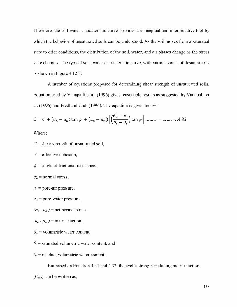
138
Therefore, the soil-water characteristic curve provides a conceptual and interpretative tool by
which the behavior of unsaturated soils can be understood. As the soil moves from a saturated
state to drier conditions, the distribution of the soil, water, and air phases change as the stress
state changes. The typical soil- water characteristic curve, with various zones of desaturations
is shown in Figure 4.12.8.
A number of equations proposed for determining shear strength of unsaturated soils.
Equation used by Vanapalli et al. (1996) gives reasonable results as suggested by Vanapalli et
al. (1996) and Fredlund et al. (1996). The equation is given below:
( ) ( ) [(
) ]
Where;
C = shear strength of unsaturated soil,
c’ = effective cohesion,
’ = angle of frictional resistance,
n = normal stress,
ua = pore-air pressure,
uw = pore-water pressure,
(n - ua ) = net normal stress,
(ua - uw ) = matric suction,
w = volumetric water content,
s = saturated volumetric water content, and
r = residual volumetric water content.
But based on Equation 3.2. and 3.23, the cyclic strength including matric suction
(Cmc) can be written as;

139
[ (
(
)
)
(
)
] ( )
The effect of water content equal to liquid limit or more brings the intrinsic aspect of
sensitive clay, which is just opposite to the matric suction. Liu and Carter (2002) gave the
relationship for the isotropic virgin compression line for the reconstituted soil, i.e., ICL*, (see
Figure 4.1.9) as;
Where; e* is the void ratio for the reconstituted clay sample. All the rest of the parameters
(Μ*, λ*,κ*, ν*& Λ*) are same as defined above except with the difference that they are
denoted with the sign of asterisk (*). Therefore, based on Equation 3.2., the intrinsic cyclic
strength (Cfc*) can be written as;
[
(
(
) )
(
)
]
The use of Modified Cam Caly Model is very helpful in estimating the design shear strength
under varying conditions of physical and mechanical parameters. Hence, the ,lowest or the
most critical value of shear strength can be selected and used to determine the factor of safety
based on the importance and type of project in sensitive clay regions
4.13 Safe Zone
As already mentioned, that one of the main objectives of the current research is to establish a
safe zone which has combined effect of both physical and mechanical parameters. The graphical
analysis shown in Figures 4.9.1 to 4.9.8 helped in establishing an average line of demarcation
140
between the failed samples and those which attain a stable position or quasi elastic resilient state
based on one of the major governing physical parameters i.e., the degree of saturation. The
degree of saturation represents the effect of other physical parameters like water content and
liquidity index. The mathematical equation for the line of demarcation between stable and failure
zones established in case degree of saturation (figures 4.9.1 to 4.9.8) gives following empirical
relationship as;
Where, a1 and b1 are constants. This expression is in good agreement with the study of Miller et
al. (2000) which is only based on single type of clay and 12 test samples. The relationship given
in equation 3.25 clearly indicates that there is a strong relationship between cyclic shear strength
and initial degree of saturation.
The graphical analysis shown in Figures 4.10.5 to 4.10.14 helped in establishing an
average line of demarcation between the failed samples and those which attain a stable position
or quasi elastic resilient state. The key parameter in this case is the number of loading cycles, N
(see section 4.11). The best fit curve which, establish the line of demarcation between stable and
failure zones can be expressed in general form as;
Where, a2 and b2 are constants.
Based on equations 3.25 & 3.26 a design safe zone can be established by selecting the
lowest values of cyclic stress ratio, hence, the resultant curve will reflect the combined effect of
both physical and mechanical parameters. In other words, by taking degree of saturation, S as a
representative of the physical parameters and number of cyclic loading, N for the mechanical
141
parameters a combined effect safe zone can be defined. Figures 4.13.1 shows the combined
effect safe zone for the experimental data of the cyclic triaxial tests. Since, the combined effect
safe zone includes the data for the Group I. II and III, therefore, most of the Group-I tests are
lying outside the range of the safe zone.
It is interesting to mention the use of Modified Cam Clay Model mentioned in section
4.12.2 at this point. By comparing curves of Figure 4.12.4 and 4.13.1, it is clear that the zones
under those curves are the safe zones. Although, the curve in Figure 4.12.4 based only on a
single Test, C20 but, it is safe to use it in the projects of extreme importance. Hence, by using of
the equations 3.32, 3.34, 3.2., 3.22 and 3.24 the minimum or the most critical value of the shear
strength can be selected to design the combined effect safe zone. Finally, based on the analysis of
experimental data, proposed hypothetical model, use of Modified Cam Clay Model and the
combined effect safe zone a summarized form of guide line is proposed in Figure 4.13.2 to
design new or examine existing foundation in sensitive clay regions.
4.14 Discussion
This study is based on a sophisticated experimental investigation and detailed analysis of the
experimental data. The static and cyclic triaxial compression tests conducted on the clays with
varying sensitivity number, along with step by step analysis of the governing physical and
mechanical parameters, assisted in exploring the complexity involved in prioritizing the role of
governing parameters on the behavior of sensitive clays subjected to static or cyclic loading.
The two main categories; physical and mechanical are considered to be the controlling
parameters for the behavior of the sensitive clay under different loading conditions. Physical
category includes parameters like; natural water content (w), liquid limit (LL), plastic limit (PL),
plasticity index (IP), liquidity index (IL), sensitivity (St), constant of variation in sensitivity (k)

142
and initial degree of saturation (S). Whereas, mechanical category includes parameters like;
cyclic deviator stress (qcyc), pore water pressure (u), axial strain (), over consolidation ratio
(OCR), preconsolidation pressure (p), confining pressure (3), and number of cycles (N).
Test analysis of the test results indicate the importance of conducting tests on both
undisturbed and remolded samples, the samples of Group-I (undisturbed) are considered stronger
than those of Group II and III (remolded samples). This holds true as far as static strength is
concerned, but the results for cyclic triaxial tests have given another view also, i.e., in case of
undisturbed sample, the rigidity of the clay skeleton restrained the buildup of large pore pressure
generation in the beginning of the test, then, as time passed by the cyclic load disturbed the clay
skeleton that is why some undisturbed samples did not show big difference in cyclic shear
strength ratio as compared to their remolded or reconstituted samples. The analysis of the data
also shows that the initial strength of undisturbed samples cannot be considered as a reliable
factor. Hence, for design purposes, it is better to rely on the remolded shear strength. The
comparison of shear between remolded samples of Group-II with those reconstituted sample of
Group-III helped in predicting shear strength of sensitive when subjected to excessive
groundwater fluctuations.
The analysis indicates the undrained triaxial test is more critical than the drained. As the
shear stress is directly proportional to an increase in pore water pressure during cyclic loading
which in turn is directly proportional to the number of cyclic loadings. Since, the undrained
cyclic loading of sensitive clay is more likely to cause effective stress failures due to a continued
increase in excessive pore water pressure as compared to drained conditions.

143
The results support the concept of threshold or critical cyclic shear stress ratio below
which no excess pore pressure will develop. When the cyclic stress ratio is higher than the
critical stress ratio, the variations of pore pressure and axial strain are different from those when
the cyclic stress ratio is lower than the critical stress ratio. The increase in normalized pore water
pressure ratio, under high confining stresses, initiate a higher normalized pore water pressure
ratios. Also, the axial strain and pore water pressure both increase with increasing number of
cyclic loading. Hence, causes stress path to move towards failure envelope. For a given
condition, the threshold cyclic shear strength is different for the clays bearing different
sensitivity number. A sample of sensitive clay subjected to cyclic loading attains and will keep
on retaining equilibrium or quasi elastic resilient state as long as the magnitude of cyclic deviator
stress is below a certain threshold level for a given degree of saturation and stress conditions
The analysis of the test data also make it clear that the decrease in the rate of loading
leads to an increase in accumulated pore pressures with respect to the number of cycles. Also, the
effect of frequency is more dominant during the initial cycles, which, diminishes progressively
as the number of cycles, N increases.
The results show that the static and cyclic shear strength is highest for the Group-I
(undisturbed samples) amongst the three groups I (Undisturbed samples), II (sample
reconstituted or remolded at same moisture content as their undisturbed parent samples Group-I)
& III (samples reconstituted at a moisture content equal to or greater than liquid limit). The static
and cyclic shear strength is least for the samples reconstituted at a moisture content equal to or
greater than liquid limit. In other words, the samples belonging to Group-III bearing intrinsic
parameters are the weakest samples among the Group I, II & III. Also, the physical and index
property test results for the sensitive clays show that the sensitivity varies with the change in the

144
natural water content and the depth from where these samples were taken. In other words,
sensitivity varies with the liquidity index and pre-consolidation pressure in these sensitive clays.
Also, the variation in sensitivity constant, k = 2 to 3 holds good for liquid limit versus sensitivity
(St) graphical analysis for the selected ranges of preconsolidation pressure.
The study shows that the rate of pore pressure build up within normally consolidated
sample is higher than that within over-consolidated sample of the same clay type. The test results
indicate that the higher the over-consolidation ratio (OCR) is, the more number of loading cycles
are needed to initiate initial liquefaction for a particular cyclic stress ratio and that the cyclic
shear strength increases with the increase in OCR. Also, the pre-consolidation pressure p in
terms of OCR is identified as an important factor in controlling the behavior of sensitive clays
especially under cyclic loading. The results of the standard consolidation test for clay samples
indicate that most of the samples belonging to depths greater than 4 m behaved like normally
consolidated clays (NCC). While, the samples belonging to shallow depths i.e., less than 3.5 m
showed over consolidation clay‟s behavior.
The analysis for establishing line of demarcation between failed and survived samples
based on the degree of saturation clearly indicate that the undrained test results give a lower limit
for the shear strength for the clay samples having degree of saturation greater than 98% or fully
saturated i.e., 100%. The test results give an idea that an undrained fully saturated test represents
the critical situation for sensitive clay subjected to cyclic loading due to complete absence of
matric suction. Moreover, the scenario becomes worst in case of a sample reconstituted at
moisture content equal to or greater than the liquid limit. In other words samples bearing intrinsic
shear strength (Cu*) under the undrained conditions represents the most critical situation. This

145
represents the field conditions where excessive rainfall along with cyclic load applications cause
rapid degradation of the foundation soil resulting into liquefaction and catastrophic failure.
The analysis identify the degree of saturation as a parameter which reflects the combined
effect of other physical parameters like; water content (w), liquid limit (LL), plastic limit (PL),
plasticity index (IP), liquidity index (IL) and constant of variation in sensitivity (k). The fact, that
the samples tested under same total stress conditions but with higher initial degree of saturation
results into failure, while the sample with comparatively lower values of initial degree of
saturation survived and attained quasi elastic resilient state gives rise to the relationship among
matric suction, initial degree of saturation cyclic shear strength and intrinsic cyclic shear strength
The analysis of data of group IV and V samples assisted in identifying the number of
cycles needed to reduce the static shear strength of an undisturbed clay sample to its remolded
strength. The analysis show that the sensitivity number for an undisturbed sensitive clay sample
does not apply to it unless and otherwise it is disturbed to an extent where its undranied
(undisturbed) shear strength reduces to a value equal to the undrained (disturbed) remolded shear
strength (cur). This analysis assisted in proposing a hypothetical model, which is useful in
depicting the shear strength of sensitive clay foundations subjected to cyclic loading. The higher
the sensitivity number faster the clay loses its shear strength under cyclic loading, through this
hypothetical model a new parameter termed as degree of remolding, r is defined.
Based on the theory of the hypothetical model a successful attempt has been made to
adapt the Modified Cam Clay Model for analyzing the behavior of the sensitive clay subjected to
cyclic loading. The adapted Modified Cam Clay Model can be used to determine the step by step
reduction in the cyclic shear strength subjected to a given set of governing parameters. The
model is useful in predicting the minimum or the most critical value of shear strength based on

146
the importance of the project. Moreover, by using the ratio of ultimate shear strength to
allowable shear strength a reliable factor of safety can be selected for designing foundations on
sensitive clays.
The relationship given in equation 3.25 clearly indicates that there is a strong relationship
between cyclic shear strength and initial degree of saturation. The degree of saturation also
identified as parameter, which can translate the effects of parameters belonging to the physical
category. On the other equation 3.26 clearly indicates that there is a strong relationship between
cyclic shear strength and number of cyclic load, N. The combination of “N” number of cycles (X
–axis) and cyclic deviator stress or deviator stress ratio (Y-axis) can easily translate the effect of
parameters belonging to the mechanical category. The analysis has shown that the combined
effect of both the categories physical and mechanical has a better definition of safe zone than the
one given by Hanna & Javed, 2008. The new safe zone is named as combined effect safe zone is
considered to be safer and more reliable in designing cyclic shear stress ratios for the foundation
design in regions of sensitive clays.

147
Figure 4.1.1: Static Triaxial Test X-Y scattered chart peak stresses versus strains
Figure 4.1.2: Static triaxial test X-Y scattered chart peak stresses versus strains

148
Figure 4.1.3:Static triaxial test X-Y scattered chart peak pore water pressure versus strains
Figure 4.1.4 Static triaxial test X-Y scattered chart peak pore water pressure versus strains

149
Figure 4.1.5 Static triaxial test typical stress-strain curves
Figure 4.1.6 Static triaxial test typical stress-strain curves

150
Figure 4.2.1 Cyclic triaxial tests X-Y scattered chart cyclic stress ratio versus axial strains
Figure 4.2.2 Cyclic triaxial tests X-Y scattered chart cyclic stress ratio versus axial strains

151
Figure 4.2.3 Cyclic triaxial tests X-Y scattered chart normalized pore water pressure
versus axial strains
Figure 4.2.4 Cyclic triaxial tests X-Y scattered chart normalized pore water pressure
versus axial strains

152
Figure 4.2.5 Cyclic deviator stress versus time ( Test ID – A 57, sample ID S-13252_ZF)
Figure 4.2.6 Pore pressure versus time (Test ID – A 57, sample ID S-13252_ZF)

153
Figure 4.2.7 Axial strain versus time ( Test ID – A 57, sample ID S-13252_ZF)
Figure 4.2.8 Cyclic deviator stress versus axial strain (Test ID – A 57, sample ID S-
13252_ZF)

154
Figure 4.2.9 Pore pressure vs axial strain( Test ID – A 57, sample ID S-13252_ZF)
Figure 4.2.10 Effective stress path (Test ID – A 57, sample ID S-13252_ZF)

155
Figure 4.3.1 Comparison of drained/undrained cyclic triaxal compression test Clay Type-C
Figure 4.4.1 Comparison of undisturbed and remolded samples Clay Type-A

156
Figure 4.4.2 Comparison of undisturbed and remolded samples Clay Type-C
Figure 4.4.3 Comparison of undisturbed and remolded samples Clay Type-C

157
Figure 4.5.1 Effect of OCR, Cyclic stress ratio versus Number of cycles Clay Type – C
Figure 4.5.2 l Pore water pressure pattern for remolded normally consolidated clay
Test ID C42 Group –II Sample ID S13048-G_BH-02

158
Figure 4.5.3 Pore water pressure pattern for an undisturbed over consolidated clay
Test ID C 31 Group –I Sample ID S13048-G_BH-02-TS
Figure 4.5.4 Degradation Index variation due to OCR – Clay Type – C

159
Figure 4.6.1 Effect of loading frequencies on undisturbed samples Clay Type – C
Figure 4.6.2 Effect of loading frequencies on remoulded samples Clay Type – C

160
Figure 4.7.1 Effect of confining pressure on cyclic deviator stress ratio w.r.t 3, Clay C
Figure 4.7.2 Effect of confining pressure on pore pressure ratio w.r.t 3, Clay Type – C

161
Figure 4.8.1 Effect of Sensitivity Number, Cyclic stress ratio versus Number of cycles
Group – I (undisturbed samples) Clay Types A, B, C & D
Figure 4.8.2 Effect of Sensitivity Number, Cyclic stress ratio versus Number of cycles
Group – II & III (Remolded samples) Clay Types A, C & D

162
Figure 4.8.3 Liquidity Index, IL versus Sensitivity Number St
Figure 4.8.4 Variation in sensitivity constant, k Liquidity Index, IL versus Sensitivity
Number St

163
Figure 4.8.5 Effect of Sensitivity constant k, Undrained shear strength versus Liquidity
Index
Figure 4.9.1 Relationship between Cyclic Stress Ratio, Degree of Saturation and Failure
Clay Type - A

164
Figure 4.9.2 Relationship between Cyclic Stress Ratio, Degree of Saturation and Failure
Clay Type – B
Figure 4.9.3 Relationship between Cyclic Stress Ratio, Degree of Saturation and Failure
Clay Type – C

165
Figure 4.9.4 Relationship between Cyclic Stress Ratio, Degree of Saturation and Failure
Clay Type – D
Figure 4.9.5 Relationship between Cyclic Stress Ratio, Degree of Saturation and Failure
Clay Overall

166
Figure 4.10.1: Deviator Stress Versus Effective Stress Test ID A8, Group – III Sample ID
S_13293-G_BH-02_TS Clay Type – A
Figure 4.10.2: Stress Path multiple levels for deviator stress versus effective stress Clay
Type-C Sample ID 13352_GE

167
Figure 4.10.3: Pore Water Pressure versus Axial Strain Test ID A8, Group – III Sample ID
S_13293-G_BH-02_TS
Figure 4.10.4 Pore Water Pressure versus Axial Strain (Clay Type-C Sample ID 13352_GE

168
Figure 4.10.5 Best fit Curves for Establishing Failure, Transition and Equilibrium
envelopes Clay Type – A
Figure 4.10.6 Best fit Curves for Establishing Failure, Transition and Equilibrium
envelopes Clay Type – B

169
Figure 4.10.7 Best fit Curves for Establishing Failure, Transition and Equilibrium
envelopes Clay Type – C
Figure 4.10.8 Best fit Curves for Establishing Failure, Transition and Equilibrium
envelopes Clay Type – D

170
Figure 4.10.9 Best fit Curves for Establishing Failure, Transition and Equilibrium
envelopes Clay Types A, B, C & D

171
Figure 4.12.1: A schematic diagram for the proposed hypothetical model
Figure 4.12.1.1: Variation of static strength after cyclic loading
(Data from; Theris and Seed, 1969)

172
Figure 4.12.1.2:Typical hysterical loops, cyclic deviator stress versus axial strains Clay A
Figure 4.12.1.3: Reduction in shear strength due to cyclic loading Clay Type – A

173
Figure 4.12.1.4: Reduction in shear strength due to cyclic loading Clay Type – C
Figure 4.12.1.5: Effect of number of Cycles on static shear strength ratio

174
Figure 4.12.1.6: Effect of number of Cycles on static shear strength ratio (log scale)
Figure 4.12.2: Consolidation and Yield of Modified Cam Clay Eekelen and Potts, (1978)

175
Figure 4.12.3 Stable state boundary surface (SSBS) in three dimensions for one particular
value of specific volumeAfter Eekelen and Potts, (1978)

176
Figure 4.12.4: Shear strength ratio versus number of cycles, N
(Test C20, sample ID 13252_ZNA)

177
Figure 4.12.5: Variation in parameter (Λ) with the number of cycles, N
(Test C20, sample ID 13252_ZNA)
Figure 4.12.6: A typical behavior of consolidating and swelling for p’-q plane
Eekelen and Potts, (1978)
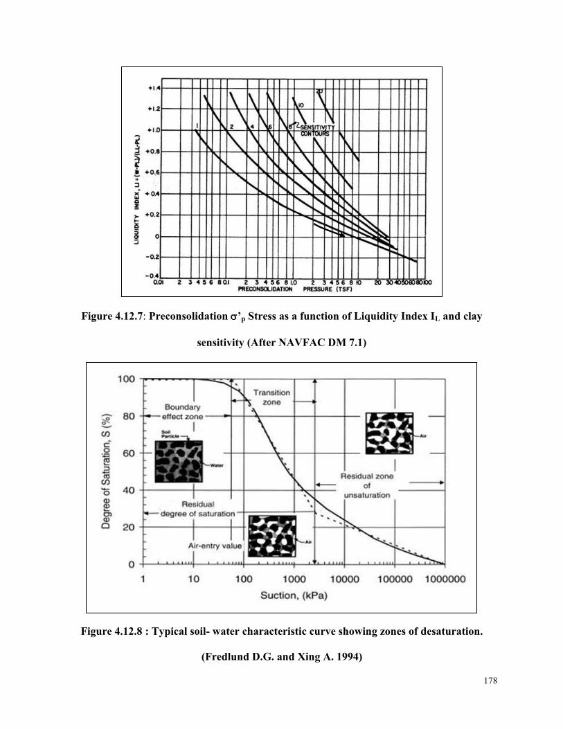
178
Figure 4.12.7: Preconsolidation ’p Stress as a function of Liquidity Index IL and clay
sensitivity (After NAVFAC DM 7.1)
Figure 4.12.8 : Typical soil- water characteristic curve showing zones of desaturation.
(Fredlund D.G. and Xing A. 1994)

179
Figure 4.12.9 A typical e-lnp curve for the undisturbed and reconstituted samples
(After Liu and Carter, 2002)
Figure 4.13.1 Designed Safe Zone based on combined effect of physical and mechanical
parameters

180
Figure 4.13.2: Flow chart for the proposed guide line to deal with new or examining
existing foundations on sensitive clay
Remolded / Reconstituted Zone

181
Chapter 5
Conclusions and Recommendations
The present research is based on a well-planned and organized experimental program to examine
the complexity of the behavior of sensitive clay subjected to cyclic loading. A detailed literature
review has identified the study gaps, and accordingly, in formulating well defined objectives for
this research. Furthermore, step by step analysis of the experimental data, keeping in view, the
complexity involved in dealing with variety of physical and mechanical parameters enhanced the
credibility of this study. Based on the results of this study, the following sections of research
contribution, limitations, conclusions and recommendations are presented.
5.1 Research Contribution
Chapter One and Two were devoted to an in-depth review of the seminal and contemporary
literature on the factors governing the behavior of a sensitive clay and how these characters
interrelate with each other when it comes to critical undrained cyclic loading conditions. With
the comprehensive overview of the previous studies along with the background of sensitive clay
and the different sources contribute in causing disturbances leading to cyclic of loading or
repeated load applications (Chapter-1), these chapters functioned to direct the research towards
an in-depth experimental exploration of comparatively unexplored issues related to the behavior
of sensitive clay subjected to cyclic loading. This thing pops up directly to the question of the
present research‟s contribution to the field the of geotechnical engineering. Some of the main
contributions of the current research in the field of geotechnical engineering are as follows;
Differentiating and prioritizing the role of physical and mechanical parameters in
governing the behavior of sensitive clay subjected to cyclic loading.

182
The development of a hypothetical model, which explains the behavior of sensitive clay
and how its shear strength reduces when subjected to disturbing / remolding action of
cyclic loading.
Developing a Modified Cam Clay Model, which is capable to predict the behavior of
sensitive clay subjected to cyclic loading.
Identify the role of the degree of saturation and the matric suction in case of partially
saturated samples on the cyclic shear strength of clay.
Establishing the safe zone concept for the cases of undrained and drained, which provide
a useful technique for designer to determine the condition of the foundation under a given
field conditions.
5.2 Limitations of Research
Some of the limitations of this study stem from the method used to obtain undisturbed samples.
Furthermore, the difficulties associated in sampling, it can be reported herein that the samples
taken for the selected types of clay A, B, C and D were not exactly from the same depths,
moreover, the quantity of samples collected for all the selected types were not same. For e.g.,
only the clay Types A and C had a represent able quantity of required samples. The samples for
Types B and D were less and most of them somehow got disturbed. The other important issue is
waxing the samples timely and properly which may lead to losing the moisture content, showing
a lower value of initial degree of saturation than the actual. As, pertains to methodological
approach, the research based on typical classical experimental work.

183
5.3 Conclusion
Based on the experimental and theoretical investigation performed on the shear strength of
sensitive clay, the following can be concluded.
The behavior of sensitive clay is governed by the four major categories of
parameters namely; physical, mechanical, environmental and chemical. For a
given region, the effect of environmental and chemical categories will remain
unchanged. This research was focused on the role of the physical and mechanical
parameters, which govern the behavior of sensitive clay subjected to static and
cyclic loading.
The Physical category includes; natural water content (w), liquid limit (LL),
plastic limit (PL), plasticity index (IP), liquidity index (IL), sensitivity (St),
constant of variation in sensitivity (k) and initial degree of saturation (S).
Whereas, mechanical category includes; cyclic deviator stress (qcyc), pore water
pressure (u), axial strain (), over consolidation ratio (OCR), preconsolidation
pressure (p), confining pressure (3), and number of cycles (N).
For a given condition, the threshold cyclic shear strength depends on the
sensitivity number. A sample of sensitive clay subjected to cyclic loading attains
and will keep on retaining equilibrium or quasi elastic resilient state as long as the
magnitude of cyclic deviator stress is below the threshold level for a given degree
of saturation and stress conditions
The effect of frequency is more dominant during the initial cycles, which,
diminishes progressively as the number of cycles, N increases. Furthermore, a

184
decrease in the rate of loading leads to an increase in the accumulated pore
pressures with respect to the number of cycles.
The intrinsic shear strength should be considered as the critical value for
estimating the strength parameters for design of the foundation.
Sensitivity number varies with the liquidity index and pre-consolidation pressures.
For design purpose, the value of sensitivity constant, k should be taken between 2
to 3 as it provides good relationship for liquid limit versus sensitivity (St) number
for the selected ranges of preconsolidation pressure. Also, the preconsolidation
pressure p in terms of OCR is an important factor in predicting the shear strength
of sensitive clays especially under cyclic loading.
The undrained fully saturated test represents the critical situation for sensitive
clay subjected to cyclic loading due to complete absence of matric suction.
The degree of saturation is a parameter represents the combined effect of the other
physical parameters such as; water content (w), liquid limit (LL), plastic limit
(PL), plasticity index (IP), liquidity index (IL) and constant of variation in
sensitivity (k).
The proposed hypothetical model together with the Modified Cam Clay Model
can be used to determine the step by step reduction in the cyclic shear strength
subjected to a given set of governing parameters.
The safe zones presented in this thesis are based on the combined effect of all the
major physical and mechanical parameters which govern the behavior of sensitive
clay subjected to static or cyclic loading.

185
The identified safe zones together with the theoretical model developed herein
constitute a valuable tool for design foundation on sensitive clay subjected to
cyclic loading. Also can be used to examine the condition of an existing
foundation.
5.4 Recommendation for the future work
Triaxial static and cyclic compression test should be attempted on partially
saturated samples, having degree of saturation ranging 50% to 90%. Such an
experimental work will help in establishing line of demarcation between samples,
which gain strength due to matric suction and the samples which become more
vulnerable to failure due to the absence of water molecules. Hence, concept of
threshold value of degree of saturation can be introduced
Using the safe zone technique and probability analysis such as “Confidence
Limits”, a comparison among the various cost effective techniques for laying new
or strengthening existing foundations on sensitive clay should be attempted.

186
REFERENCES
Ansal, M. and Erken, A. 1989. Undrained Behavior of Clay under Cyclic Shear Stresses.
ASCE, Journal of Geotechnical Engineering, 115 (7), pp 968-981.
Bjerrum, L., 1954. Geotechnical Properties of Norwegian Marine Clays. Geotechnique, 4
(2), pp. 49-69.
Berre, T. (1981). Triaxial testing at NGI. Geotechnical Testing Journal, Vol. 5, 1982, No.
1/2, pp. 3-17.
Chagnon, J.Y., Lebuis, J., Allard, J.D. and Robert, J.M. 1979. Sensitive Clays, Unstable
Slopes, Corrective works and Slides in the Quebec and Shawinigan Area. Geological Association
of Canada.
Das, Braja, M., Fundamentals of Soil Dynamics, Elver Science Publishers Co., Inc, New
York, NY, 1983
Das, Braja, M. (2001). Priciples of Geotecnical Engineering” Fifth Edition,
Eden, WJ, 1971. Sampler Trials in Overconsolidated Sensitive Clay Research Council of
Canada, Ont.
Eekelen, H.A.M., and Potts, D.M., 1978. The behavior of Drammen Clay under cyclic
loading. Geotechnique 28 (2), pp. 173-196.
Erken, A., and Ulker, C., 2006 Effect of cyclic loading on monotonic shear strength of
fine-grained soils. Engineering Geology Volume 89, Issues 3-4, 6. Accepted 25 October 2006.,
Pages 243-257

187
Finn, W. D. Liam, Aspects of Constant Volume Cyclic Simple Shear, Advances in the
Art of Testing Soils Under Cyclic Conditions, American Society of Civil Engineers, New York,
NY, 1985
Fredlund D.G. and Xing A. 1994. Equations for the soil characteristics curve. Canada
Geotechnical Journal J. 31. 521-532
Hanna, A.M., and Javid, K. 2008. Foundations on Sensitive Clay Subjected to Cyclic
Loading. ASCE, Journal of Geotechnical and Geo-environmental Engineering, 134 (7)
Houstan, W.N., and Hermann, H.G., 1980. Undrained Cyclic Strength of Marine Soils.
Journal of Geotechnical Engineering. 106, No. GT6, pp. 691-711.
Hyodo, M., Yamamoto, Y., and Sugiyama, M., 1994. Undrained cyclic shear behavior of
normally consolidated clay subjected to initial static shear stress. Soil and Foundations 34 (4),
pp. 1-11.
Iwasaki, T., Tatsuoka, F., and Takagi, Y. 1978. Shear modulus of sands under cyclic
torsional shear loading," Soils and Found. 18 (1), pp. 39-50
J, Zhou., and X, Gong., 2001. Strain degradation of saturated clay under cyclic loading.
Canadian Geotechnical Journal, Volume 38, Number 1, February 2001 , pp. 208-212(5)
Lacasse, S. and T. Berre (1988). Triaxial testing methods for soils. State-of-the-art paper.
ASTM, Special Technical Publication, 977, pp. 264-289.
Lefebvre, G., and LeBoeuf, D., 1987. Rate Effects and Cyclic Loading of Sensitive
Clays. Journal of Geotechnical Engineering, 113 (5), pp. 476-489.
Lefebvre, G., and Pfendler, P., 1996. Strain Rate and Pre-Shear Effects in Cyclic
Resistance of Soft Clay. ASCE, Journal of Geotechnical Engineering, 122 (1), pp. 21-26.

188
(Lefebvre and Poulin 1979). CHAPTER 3 sherbrooke sampler……………….
Leroueil, S., Tavenas, F., and Le Bihan, J.P. 1983. Propriétés caractéristiques des argiles
de l‟est du Canada. Canadian Geotechnical Journal, 20(4): 681–705.
Li, Tao., and Meissner Helmut., 2002. Two-Surface Plasticity Model for Cyclic
Undrained Behavior of Clays. . Geotech. and Geoenvir. Engrg., Volume 128, Issue 7, pp. 613-
626 (July 2002)
Liang, R.Y., and Ma, F., 1991. Anisotropic plasticity Model for Undrained Cyclic
Behavior of Clays. Journal of Geotechnical Engineering, 118 (2), pp. 229-243.
Liu, Martin D and Carter, John P., 2002. A Structured Cam Clay Model. Center of
Geotechnical Research, Report No R814.
Matsui, T. Ohara, H., and Itlo, T. 1980. Cyclic stress-strain history and shear
characteristics of clays. ASCE, Journal Geotechnical Engineering, 106 (10) pp. 1101-1120.
McK Yes,E., Sethi, A. And Yong, R.N. 1973. Amorphous Coatings on Particles of
Sensitive Clay Soils.Clay and Clay Minerals, Vol. 22, pp. 427 – 433.
Miller. G.A., The, S.Y., Li, D., and Zaman, M.M., 2000. Cyclic Shear Strength of Soft
Railroad Subgrade. ASCE, Journal of Geotechnical and Geoenvironmental Engineering, 126 (2),
pp. 139-147.
Min, CHEN Yun., Mei-xiu, JI., and Bo, H., 2004. Effect of Cyclic Loading Frequency
on Undrained Behaviors of Undisturbed Marine Clay. Journal-China Ocean Engineering 2004.
Oak, Fusao,. Takeshi Kodaka, Takeshi., and 1
, Kim, Yong-Seong., 2003. A cyclic
viscoelastic-viscoplastic constitutive model for clay and liquefaction analysis of multi-layered

189
ground. 1
Department of Civil and Earth Resources Engineering, Graduate School of Engineering,
Kyoto University, Yoshida Hon-machi, Sakyo-ku, Kyoto 606-8501, Japan.
Prakash, Shamsher, Soil Dynamics, McGraw-Hill, Inc., 1981
Procter, D.C., and Khaffaf, J.H., 1984. Weakening of Undrained Saturated Clays Under
Cyclic Loading. Journal of Geotechnical Engineering, Vol. 110, No. 10, pp. 1431-1445.
Reilly, M.P.O and Brown, S.F. 1991. Cyclic Loading of Soils: “From Theory to Design”
Sangrey, D. A., Henckel, D.J., and Esring, M.L., 1969. The Effective Stress Response of
a Saturated Clay Soil to Repeated Loading. Canadian Geotechnical Journal, 6 (3), pp. 241-251.
Seed, H.B., and Idriss, I.M., 1981. Ground Motions and Soil Liquefaction During
Earthquakes, Earthquake Engineering Research Institute, Oakland, California, Monograph
Series, pp. 134.
Silvestri V, 1994. Water Content Relationships of a Sensitive Clay Subjected to Cycles of
Capillary Pressures, Volume Geotechnical Testing Journal, Vol. 17, Issue 1 (March 1994).
Silvestri V, 1981. Behavior of an Overconsolidated Sensitive Clay in Drained K0-Triaxial
Tests, Assistant Professor, Department of Civil Engineering, Ecole Polytechnique, P. Q.
Published: Jan 1981
Skempton, A.W., 1957. A contribution to the settlement Analysis of Foundations on
Clay. Geotechnique, 7 (1), pp. 168.
Wood, D.M., 1990. Soil Behavior and Critical State Soil Mechanics. Cambridge University
Press.

190
Scholey GK, Frost JD, Lo Presti DCF, Jamiolkowski M, A Review of Instrumentation for
Measuring Small Strains During Triaxial Testing of Soil Specimens, ASTM Geotechnical
Testing Journal, Vol 18, No. 2, pp. 137- 156, 1995.
Thammathiwat, A., and Chim-oye, W., 2004. Behavior of Strength and Pore Pressure of
Soft Bangkok Clay under Cyclic Loading. Journal of Science and Technology, Vol. 9, No. 4,
October-December 2004
Theris, G.R., and Seed, H.B., 1969. “Strength and Stress – Strain Characteristics of Clays
Subjected to Seismic Loading Conditions.” Vibration Effects of Earthqaukes on Soils and
Foundations, Special Technical Publication 450, ASTM, 1969. Pp. 3-56.
Terzaghi Karl, Brazelton Ralph and Mesri Gholamreza (1944/1947) Published third
edition 1995. “ Soil Mechanics in Engineering Practice”
Vinod K. Garga, Mahbubul A. Khan and Sai K. Vanapalli (2005)Stress-path dependent
behavior of a weathered clay crust Department of Civil Engineering, University of Ottawa, 161
Louis Pasteur, Ottawa, Ontario, K1N 6N5, Canada
Yu, H. S. (1997). A unified state parameter model for clay and sand. Department of Civil
Engineering and Surveying. University of Newcastle, N.S.W. 2308, Australia.

i
APPENDIX –I
Cyclic loading Model for Sensitive Clay
Use of Modified Cam Clay Model
Cyclic Triaxial Compression Test
Test Id C20 Sample Id 13252_ZNA-

ii
Hanna & Constt Variable Constt Variable
Javed, 2008 Λ Λ Λ Λ
N ЄA u F.O.S F.O.S F.O.S b b Λ
I II III
1 0.00 0.00 1.45 1.26 1.30 0.630 0.641 0.0450
2 0.21 0.40 1.36 1.26 1.30 0.630 0.640 0.7868
3 0.21 11.74 1.31 1.26 1.29 0.630 0.640 0.7871
4 0.22 28.29 1.28 1.25 1.28 0.630 0.639 0.7877
5 0.22 43.46 1.26 1.24 1.26 0.630 0.639 0.7877
6 0.23 51.05 1.24 1.23 1.26 0.630 0.639 0.7880
7 0.23 60.70 1.22 1.23 1.25 0.630 0.639 0.7882
8 0.23 68.97 1.21 1.22 1.24 0.630 0.639 0.7882
9 0.23 77.25 1.19 1.21 1.23 0.630 0.639 0.7882
10 0.24 83.45 1.18 1.21 1.23 0.630 0.639 0.7885
11 0.24 93.79 1.17 1.20 1.22 0.630 0.638 0.7887
12 0.25 104.14 1.16 1.19 1.21 0.630 0.638 0.7890
13 0.25 104.14 1.16 1.19 1.21 0.630 0.638 0.7890
14 0.25 115.17 1.15 1.18 1.19 0.630 0.638 0.7892
15 0.25 115.17 1.14 1.18 1.19 0.630 0.638 0.7892
16 0.25 122.06 1.13 1.17 1.18 0.630 0.638 0.7892
17 0.25 122.06 1.13 1.17 1.18 0.630 0.638 0.7892
18 0.26 129.65 1.12 1.16 1.17 0.630 0.638 0.7894
19 0.25 135.16 1.12 1.15 1.17 0.630 0.638 0.7892
20 0.26 138.61 1.11 1.15 1.16 0.630 0.638 0.7894
21 0.26 139.99 1.11 1.15 1.16 0.630 0.638 0.7894
22 0.26 144.82 1.10 1.14 1.15 0.630 0.638 0.7896
23 0.26 144.82 1.10 1.14 1.15 0.630 0.638 0.7896
24 0.26 144.82 1.09 1.14 1.15 0.630 0.638 0.7896
25 0.26 153.09 1.09 1.13 1.14 0.630 0.638 0.7896
26 0.27 155.16 1.09 1.12 1.13 0.630 0.638 0.7898
27 0.27 155.16 1.08 1.12 1.13 0.630 0.638 0.7898
28 0.27 157.92 1.08 1.12 1.13 0.630 0.638 0.7898
29 0.27 164.12 1.08 1.11 1.11 0.630 0.638 0.7898
30 0.27 164.12 1.07 1.11 1.11 0.630 0.638 0.7900
31 0.27 165.50 1.07 1.10 1.11 0.630 0.638 0.7900
32 0.27 166.88 1.07 1.10 1.11 0.630 0.638 0.7900
33 0.27 166.88 1.06 1.10 1.11 0.630 0.638 0.7900
34 0.27 173.09 1.06 1.09 1.09 0.630 0.638 0.7900
35 0.28 173.09 1.06 1.09 1.09 0.630 0.637 0.7901
36 0.28 175.85 1.06 1.08 1.09 0.630 0.637 0.7901
37 0.28 175.85 1.05 1.08 1.09 0.630 0.637 0.7901
38 0.28 175.85 1.05 1.08 1.09 0.630 0.637 0.7901
39 0.28 177.22 1.05 1.08 1.08 0.630 0.637 0.7903
40 0.28 177.22 1.05 1.08 1.08 0.630 0.637 0.7903
41 0.28 177.91 1.04 1.07 1.08 0.630 0.637 0.7903
42 0.28 177.91 1.04 1.07 1.08 0.630 0.637 0.7903
43 0.28 177.91 1.04 1.07 1.08 0.630 0.637 0.7903
44 0.28 184.12 1.04 1.05 1.06 0.630 0.637 0.7903
45 0.28 184.12 1.04 1.05 1.06 0.630 0.637 0.7903
46 0.29 184.12 1.03 1.05 1.06 0.630 0.637 0.7905
47 0.29 184.12 1.03 1.05 1.06 0.630 0.637 0.7905
48 0.29 186.88 1.03 1.05 1.05 0.630 0.637 0.7905
49 0.29 186.88 1.03 1.05 1.05 0.630 0.637 0.7905
50 0.29 186.88 1.03 1.05 1.05 0.630 0.637 0.7905
51 0.29 186.88 1.02 1.05 1.05 0.630 0.637 0.7907
52 0.29 186.88 1.02 1.05 1.05 0.630 0.637 0.7905
53 0.29 188.95 1.02 1.04 1.04 0.630 0.637 0.7905
54 0.29 188.95 1.02 1.04 1.04 0.630 0.637 0.7907
55 0.29 188.95 1.02 1.04 1.04 0.630 0.637 0.7905
56 0.29 196.53 1.02 1.00 1.00 0.630 0.637 0.7907
57 0.29 196.53 1.01 1.00 1.00 0.630 0.637 0.7907
58 0.29 196.53 1.01 1.00 1.00 0.630 0.637 0.7907
59 0.29 196.53 1.01 1.00 1.00 0.630 0.637 0.7907
60 0.29 196.53 1.01 1.00 1.00 0.630 0.637 0.7907
61 0.29 196.53 1.01 1.00 1.00 0.630 0.637 0.7907
62 0.29 196.53 1.01 1.00 1.00 0.630 0.637 0.7907
63 0.29 196.53 1.01 1.00 1.00 0.630 0.637 0.7907
64 0.30 196.53 1.00 1.00 1.00 0.630 0.637 0.7908
65 0.30 196.53 1.00 1.00 1.00 0.630 0.637 0.7908
66 0.30 196.53 1.00 1.00 1.00 0.630 0.637 0.7908
67 0.30 196.53 1.00 1.00 1.00 0.630 0.637 0.7908
LO
AD
ING
-ZE
RO
DE
VIA
TO
R S
TR
ES
S

iii
Hanna & Constt Variable Constt Variable
Javed, 2008 Λ Λ Λ Λ
N ЄA u F.O.S F.O.S F.O.S b b Λ
I II III
1 0.19 0.30 1.45 1.26 1.30 0.630 0.641 0.7858
2 0.23 0.40 1.36 1.26 1.29 0.630 0.639 0.7882
3 0.25 17.26 1.31 1.25 1.28 0.630 0.638 0.7890
4 0.25 31.05 1.28 1.25 1.27 0.630 0.638 0.7892
5 0.26 44.15 1.26 1.24 1.26 0.630 0.638 0.7894
6 0.26 51.05 1.24 1.23 1.25 0.630 0.638 0.7896
7 0.27 64.84 1.22 1.22 1.24 0.630 0.638 0.7898
8 0.27 68.97 1.21 1.22 1.24 0.630 0.638 0.7900
9 0.27 77.25 1.19 1.21 1.23 0.630 0.638 0.7900
10 0.27 83.45 1.18 1.21 1.23 0.630 0.638 0.7900
11 0.28 93.79 1.17 1.20 1.21 0.630 0.637 0.7901
12 0.28 104.14 1.16 1.19 1.20 0.630 0.637 0.7901
13 0.29 104.14 1.16 1.19 1.20 0.630 0.637 0.7907
14 0.29 115.17 1.15 1.18 1.19 0.630 0.637 0.7907
15 0.29 115.17 1.14 1.18 1.19 0.630 0.637 0.7907
16 0.29 122.06 1.13 1.17 1.18 0.630 0.637 0.7907
17 0.29 129.65 1.13 1.16 1.17 0.630 0.637 0.7905
18 0.30 135.16 1.12 1.15 1.16 0.630 0.637 0.7908
19 0.30 135.16 1.12 1.15 1.16 0.630 0.637 0.7908
20 0.30 138.61 1.11 1.15 1.16 0.630 0.637 0.7908
21 0.30 139.99 1.11 1.15 1.16 0.630 0.637 0.7910
22 0.30 144.82 1.10 1.14 1.15 0.630 0.637 0.7910
23 0.30 144.82 1.10 1.14 1.15 0.630 0.637 0.7910
24 0.30 144.82 1.09 1.14 1.15 0.630 0.637 0.7910
25 0.30 153.09 1.09 1.13 1.13 0.630 0.637 0.7910
26 0.31 155.16 1.09 1.12 1.13 0.630 0.637 0.7911
27 0.31 155.16 1.08 1.12 1.13 0.630 0.637 0.7912
28 0.31 157.92 1.08 1.12 1.13 0.630 0.637 0.7912
29 0.31 164.12 1.08 1.11 1.11 0.630 0.637 0.7912
30 0.31 164.12 1.07 1.11 1.11 0.630 0.637 0.7912
31 0.31 165.50 1.07 1.10 1.11 0.630 0.637 0.7912
32 0.32 166.88 1.07 1.10 1.11 0.630 0.636 0.7914
33 0.32 166.88 1.06 1.10 1.11 0.630 0.636 0.7914
34 0.32 173.09 1.06 1.09 1.09 0.630 0.636 0.7914
35 0.32 173.09 1.06 1.09 1.09 0.630 0.636 0.7914
36 0.32 175.85 1.06 1.08 1.08 0.630 0.636 0.7915
37 0.32 175.85 1.05 1.08 1.08 0.630 0.636 0.7915
38 0.32 175.85 1.05 1.08 1.08 0.630 0.636 0.7915
39 0.32 177.22 1.05 1.08 1.08 0.630 0.636 0.7915
40 0.32 177.22 1.05 1.08 1.08 0.630 0.636 0.7915
41 0.33 177.91 1.04 1.07 1.08 0.630 0.636 0.7916
42 0.33 177.91 1.04 1.07 1.08 0.630 0.636 0.7916
43 0.33 177.91 1.04 1.07 1.08 0.630 0.636 0.7916
44 0.33 184.12 1.04 1.05 1.06 0.630 0.636 0.7916
45 0.33 184.12 1.04 1.05 1.06 0.630 0.636 0.7916
46 0.33 184.12 1.03 1.05 1.06 0.630 0.636 0.7916
47 0.33 184.12 1.03 1.05 1.06 0.630 0.636 0.7918
48 0.33 186.88 1.03 1.05 1.05 0.630 0.636 0.7918
49 0.33 186.88 1.03 1.05 1.05 0.630 0.636 0.7918
50 0.33 186.88 1.03 1.05 1.05 0.630 0.636 0.7918
51 0.33 186.88 1.02 1.05 1.05 0.630 0.636 0.7918
52 0.33 186.88 1.02 1.05 1.05 0.630 0.636 0.7918
53 0.33 188.95 1.02 1.04 1.04 0.630 0.636 0.7918
54 0.33 188.95 1.02 1.04 1.04 0.630 0.636 0.7918
55 0.34 188.95 1.02 1.04 1.04 0.630 0.636 0.7919
56 0.34 196.53 1.02 1.00 1.00 0.630 0.636 0.7919
57 0.34 196.53 1.01 1.00 1.00 0.630 0.636 0.7919
58 0.33 196.53 1.01 1.00 1.00 0.630 0.636 0.7918
59 0.34 196.53 1.01 1.00 1.00 0.630 0.636 0.7919
60 0.34 196.53 1.01 1.00 1.00 0.630 0.636 0.7919
61 0.35 196.53 1.01 1.00 1.00 0.630 0.636 0.7921
62 0.34 196.53 1.01 1.00 1.00 0.630 0.636 0.7919
63 0.34 196.53 1.01 1.00 1.00 0.630 0.636 0.7920
64 0.34 196.53 1.00 1.00 1.00 0.630 0.636 0.7920
65 0.34 196.53 1.00 1.00 1.00 0.630 0.636 0.7920
66 0.34 196.53 1.00 1.00 1.00 0.630 0.636 0.7920
67 0.34 196.53 1.00 1.00 1.00 0.630 0.636 0.7920
LO
AD
ING
- D
EV
IAT
OR
ST
RE
SS
= 2
0 k
Pa

iv
Hanna & Constt Variable Constt Variable
Javed, 2008 Λ Λ Λ Λ
N ЄA u F.O.S F.O.S F.O.S b b Λ
I II III
1 0.25 0.30 1.45 1.26 1.29 0.630 0.638 0.7892
2 0.29 0.40 1.36 1.26 1.29 0.630 0.637 0.7907
3 0.30 17.26 1.31 1.25 1.28 0.630 0.637 0.7910
4 0.31 31.05 1.28 1.25 1.27 0.630 0.637 0.7911
5 0.31 51.05 1.26 1.23 1.25 0.630 0.637 0.7912
6 0.32 51.05 1.24 1.23 1.25 0.630 0.636 0.7914
7 0.32 64.84 1.22 1.22 1.24 0.630 0.636 0.7915
8 0.33 77.25 1.21 1.21 1.23 0.630 0.636 0.7916
9 0.33 79.31 1.19 1.21 1.23 0.630 0.636 0.7916
10 0.33 93.79 1.18 1.20 1.21 0.630 0.636 0.7916
11 0.33 93.79 1.17 1.20 1.21 0.630 0.636 0.7918
12 0.34 104.14 1.16 1.19 1.20 0.630 0.636 0.7919
13 0.34 111.03 1.16 1.18 1.19 0.630 0.636 0.7920
14 0.35 115.17 1.15 1.18 1.19 0.630 0.636 0.7921
15 0.35 120.69 1.14 1.17 1.18 0.630 0.636 0.7921
16 0.35 122.06 1.13 1.17 1.18 0.630 0.636 0.7921
17 0.35 129.65 1.13 1.16 1.17 0.630 0.636 0.7922
18 0.35 135.16 1.12 1.15 1.16 0.630 0.636 0.7922
19 0.35 135.16 1.12 1.15 1.16 0.630 0.636 0.7922
20 0.35 138.61 1.11 1.15 1.16 0.630 0.636 0.7922
21 0.36 139.99 1.11 1.15 1.15 0.630 0.636 0.7923
22 0.36 144.82 1.10 1.14 1.15 0.630 0.636 0.7923
23 0.36 144.82 1.10 1.14 1.15 0.630 0.636 0.7925
24 0.36 153.09 1.09 1.13 1.13 0.630 0.636 0.7925
25 0.36 153.09 1.09 1.13 1.13 0.630 0.636 0.7925
26 0.37 155.16 1.09 1.12 1.13 0.630 0.636 0.7926
27 0.37 155.16 1.08 1.12 1.13 0.630 0.636 0.7926
28 0.37 157.92 1.08 1.12 1.12 0.630 0.636 0.7927
29 0.37 164.12 1.08 1.11 1.11 0.630 0.636 0.7927
30 0.37 164.12 1.07 1.11 1.11 0.630 0.636 0.7927
31 0.37 165.50 1.07 1.10 1.11 0.630 0.636 0.7927
32 0.37 166.88 1.07 1.10 1.11 0.630 0.636 0.7927
33 0.37 166.88 1.06 1.10 1.11 0.630 0.636 0.7927
34 0.37 173.09 1.06 1.09 1.09 0.630 0.636 0.7927
35 0.38 173.09 1.06 1.09 1.09 0.630 0.635 0.7927
36 0.38 175.85 1.06 1.08 1.08 0.630 0.635 0.7927
37 0.38 175.85 1.05 1.08 1.08 0.630 0.635 0.7927
38 0.38 175.85 1.05 1.08 1.08 0.630 0.635 0.7928
39 0.38 177.22 1.05 1.08 1.08 0.630 0.635 0.7927
40 0.38 177.91 1.05 1.07 1.08 0.630 0.635 0.7928
41 0.39 177.91 1.04 1.07 1.08 0.630 0.635 0.7929
42 0.38 177.91 1.04 1.07 1.08 0.630 0.635 0.7928
43 0.39 177.91 1.04 1.07 1.08 0.630 0.635 0.7929
44 0.39 184.12 1.04 1.05 1.06 0.630 0.635 0.7929
45 0.39 184.12 1.04 1.05 1.06 0.630 0.635 0.7929
46 0.39 184.12 1.03 1.05 1.06 0.630 0.635 0.7929
47 0.39 184.12 1.03 1.05 1.06 0.630 0.635 0.7929
48 0.39 186.88 1.03 1.05 1.05 0.630 0.635 0.7929
49 0.38 186.88 1.03 1.05 1.05 0.630 0.635 0.7927
50 0.39 186.88 1.03 1.05 1.05 0.630 0.635 0.7930
51 0.39 186.88 1.02 1.05 1.05 0.630 0.635 0.7929
52 0.39 186.88 1.02 1.05 1.05 0.630 0.635 0.7930
53 0.39 188.95 1.02 1.04 1.04 0.630 0.635 0.7930
54 0.39 188.95 1.02 1.04 1.04 0.630 0.635 0.7930
55 0.39 188.95 1.02 1.04 1.04 0.630 0.635 0.7930
56 0.40 196.53 1.02 1.00 1.00 0.630 0.635 0.7931
57 0.40 196.53 1.01 1.00 1.00 0.630 0.635 0.7931
58 0.40 196.53 1.01 1.00 1.00 0.630 0.635 0.7931
59 0.40 196.53 1.01 1.00 1.00 0.630 0.635 0.7931
60 0.40 196.53 1.01 1.00 1.00 0.630 0.635 0.7932
61 0.40 196.53 1.01 1.00 1.00 0.630 0.635 0.7932
62 0.40 196.53 1.01 1.00 1.00 0.630 0.635 0.7932
63 0.40 196.53 1.01 1.00 1.00 0.630 0.635 0.7932
64 0.40 196.53 1.00 1.00 1.00 0.630 0.635 0.7932
65 0.40 196.53 1.00 1.00 1.00 0.630 0.635 0.7932
66 0.40 196.53 1.00 1.00 1.00 0.630 0.635 0.7932
67 0.40 196.53 1.00 1.00 1.00 0.630 0.635 0.7932
LO
AD
ING
- D
EV
IAT
OR
ST
RE
SS
= 4
0 k
Pa

v
Hanna & Constt Variable Constt Variable
Javed, 2008 Λ Λ Λ Λ
N ЄA u F.O.S F.O.S F.O.S b b Λ
I II III
1 0.33 0.30 1.45 1.26 1.28 0.630 0.636 0.7918
2 0.34 11.74 1.36 1.26 1.28 0.630 0.636 0.7920
3 0.35 28.29 1.31 1.25 1.26 0.630 0.636 0.7922
4 0.36 42.77 1.28 1.24 1.25 0.630 0.636 0.7923
5 0.36 51.05 1.26 1.23 1.25 0.630 0.636 0.7925
6 0.37 60.70 1.24 1.23 1.24 0.630 0.636 0.7926
7 0.37 67.59 1.22 1.22 1.23 0.630 0.636 0.7926
8 0.37 77.25 1.21 1.21 1.23 0.630 0.636 0.7927
9 0.38 79.31 1.19 1.21 1.22 0.630 0.635 0.7927
10 0.38 93.79 1.18 1.20 1.21 0.630 0.635 0.7928
11 0.38 104.14 1.17 1.19 1.20 0.630 0.635 0.7928
12 0.39 104.14 1.16 1.19 1.20 0.630 0.635 0.7929
13 0.39 111.03 1.16 1.18 1.19 0.630 0.635 0.7929
14 0.39 115.17 1.15 1.18 1.19 0.630 0.635 0.7929
15 0.39 120.69 1.14 1.17 1.18 0.630 0.635 0.7930
16 0.39 122.06 1.13 1.17 1.18 0.630 0.635 0.7930
17 0.40 129.65 1.13 1.16 1.17 0.630 0.635 0.7931
18 0.40 135.16 1.12 1.15 1.16 0.630 0.635 0.7931
19 0.40 138.61 1.12 1.15 1.16 0.630 0.635 0.7932
20 0.40 138.61 1.11 1.15 1.16 0.630 0.635 0.7932
21 0.40 139.99 1.11 1.15 1.15 0.630 0.635 0.7932
22 0.40 144.82 1.10 1.14 1.15 0.630 0.635 0.7932
23 0.41 144.82 1.10 1.14 1.15 0.630 0.635 0.7933
24 0.41 153.09 1.09 1.13 1.13 0.630 0.635 0.7934
25 0.41 155.16 1.09 1.12 1.13 0.630 0.635 0.7934
26 0.41 155.16 1.09 1.12 1.13 0.630 0.635 0.7934
27 0.41 157.92 1.08 1.12 1.12 0.630 0.635 0.7934
28 0.42 164.12 1.08 1.11 1.11 0.630 0.635 0.7934
29 0.42 164.12 1.08 1.11 1.11 0.630 0.635 0.7934
30 0.42 165.50 1.07 1.10 1.11 0.630 0.635 0.7934
31 0.42 166.88 1.07 1.10 1.10 0.630 0.635 0.7934
32 0.42 166.88 1.07 1.10 1.10 0.630 0.635 0.7935
33 0.42 173.09 1.06 1.09 1.09 0.630 0.635 0.7935
34 0.42 173.09 1.06 1.09 1.09 0.630 0.635 0.7935
35 0.42 175.85 1.06 1.08 1.08 0.630 0.635 0.7935
36 0.42 175.85 1.06 1.08 1.08 0.630 0.635 0.7935
37 0.42 175.85 1.05 1.08 1.08 0.630 0.635 0.7935
38 0.42 177.22 1.05 1.08 1.08 0.630 0.635 0.7935
39 0.43 177.22 1.05 1.08 1.08 0.630 0.635 0.7936
40 0.43 177.91 1.05 1.07 1.08 0.630 0.635 0.7936
41 0.43 177.91 1.04 1.07 1.08 0.630 0.635 0.7936
42 0.43 177.91 1.04 1.07 1.08 0.630 0.635 0.7936
43 0.43 177.91 1.04 1.07 1.08 0.630 0.635 0.7936
44 0.43 184.12 1.04 1.05 1.06 0.630 0.635 0.7937
45 0.43 184.12 1.04 1.05 1.06 0.630 0.635 0.7937
46 0.43 184.12 1.03 1.05 1.06 0.630 0.635 0.7937
47 0.43 184.12 1.03 1.05 1.06 0.630 0.635 0.7937
48 0.44 186.88 1.03 1.05 1.05 0.630 0.635 0.7937
49 0.43 186.88 1.03 1.05 1.05 0.630 0.635 0.7937
50 0.43 186.88 1.03 1.05 1.05 0.630 0.635 0.7937
51 0.44 186.88 1.02 1.05 1.05 0.630 0.635 0.7937
52 0.44 188.95 1.02 1.04 1.04 0.630 0.635 0.7937
53 0.44 188.95 1.02 1.04 1.04 0.630 0.635 0.7937
54 0.44 188.95 1.02 1.04 1.04 0.630 0.635 0.7937
55 0.44 188.95 1.02 1.04 1.04 0.630 0.635 0.7937
56 0.44 196.53 1.02 1.00 1.00 0.630 0.635 0.7938
57 0.44 196.53 1.01 1.00 1.00 0.630 0.635 0.7938
58 0.44 196.53 1.01 1.00 1.00 0.630 0.635 0.7938
59 0.44 196.53 1.01 1.00 1.00 0.630 0.635 0.7938
60 0.44 196.53 1.01 1.00 1.00 0.630 0.635 0.7938
61 0.45 196.53 1.01 1.00 1.00 0.630 0.635 0.7939
62 0.45 196.53 1.01 1.00 1.00 0.630 0.635 0.7939
63 0.45 196.53 1.01 1.00 1.00 0.630 0.635 0.7939
64 0.45 196.53 1.00 1.00 1.00 0.630 0.635 0.7939
65 0.45 196.53 1.00 1.00 1.00 0.630 0.635 0.7939
66 0.45 196.53 1.00 1.00 1.00 0.630 0.635 0.7939
67 0.45 196.53 1.00 1.00 1.00 0.630 0.635 0.7939
LO
AD
ING
- D
EV
IAT
OR
ST
RE
SS
= 6
5 k
Pa

vi
Hanna & Constt Variable Constt Variable
Javed, 2008 Λ Λ Λ Λ
N ЄA u F.O.S F.O.S F.O.S b b Λ
I II III
1 0.205 0.40 1.45 1.26 1.30 0.630 0.640 0.7868
2 0.21 11.74 1.36 1.26 1.29 0.630 0.640 0.7871
3 0.22 28.29 1.31 1.25 1.28 0.630 0.639 0.7877
4 0.22 43.46 1.28 1.24 1.26 0.630 0.639 0.7877
5 0.225 51.05 1.26 1.23 1.26 0.630 0.639 0.7880
6 0.23 60.70 1.24 1.23 1.25 0.630 0.639 0.7882
7 0.23 68.97 1.22 1.22 1.24 0.630 0.639 0.7882
8 0.23 77.25 1.21 1.21 1.23 0.630 0.639 0.7882
9 0.235 83.45 1.19 1.21 1.23 0.630 0.639 0.7885
10 0.24 93.79 1.18 1.20 1.22 0.630 0.638 0.7887
11 0.245 104.14 1.17 1.19 1.21 0.630 0.638 0.7890
12 0.245 104.14 1.16 1.19 1.21 0.630 0.638 0.7890
13 0.25 115.17 1.16 1.18 1.19 0.630 0.638 0.7892
14 0.25 115.17 1.15 1.18 1.19 0.630 0.638 0.7892
15 0.25 122.06 1.14 1.17 1.18 0.630 0.638 0.7892
16 0.25 122.06 1.13 1.17 1.18 0.630 0.638 0.7892
17 0.255 129.65 1.13 1.16 1.17 0.630 0.638 0.7894
18 0.25 135.16 1.12 1.15 1.17 0.630 0.638 0.7892
19 0.255 138.61 1.12 1.15 1.16 0.630 0.638 0.7894
20 0.255 139.99 1.11 1.15 1.16 0.630 0.638 0.7894
21 0.26 144.82 1.11 1.14 1.15 0.630 0.638 0.7896
22 0.26 144.82 1.10 1.14 1.15 0.630 0.638 0.7896
23 0.26 144.82 1.10 1.14 1.15 0.630 0.638 0.7896
24 0.26 153.09 1.09 1.13 1.14 0.630 0.638 0.7896
25 0.265 155.16 1.09 1.12 1.13 0.630 0.638 0.7898
26 0.265 155.16 1.09 1.12 1.13 0.630 0.638 0.7898
27 0.265 157.92 1.08 1.12 1.13 0.630 0.638 0.7898
28 0.265 164.12 1.08 1.11 1.11 0.630 0.638 0.7898
29 0.27 164.12 1.08 1.11 1.11 0.630 0.638 0.7900
30 0.27 165.50 1.07 1.10 1.11 0.630 0.638 0.7900
31 0.27 166.88 1.07 1.10 1.11 0.630 0.638 0.7900
32 0.27 166.88 1.07 1.10 1.11 0.630 0.638 0.7900
33 0.27 173.09 1.06 1.09 1.09 0.630 0.638 0.7900
34 0.275 173.09 1.06 1.09 1.09 0.630 0.637 0.7901
35 0.275 175.85 1.06 1.08 1.09 0.630 0.637 0.7901
36 0.275 175.85 1.06 1.08 1.09 0.630 0.637 0.7901
37 0.275 175.85 1.05 1.08 1.09 0.630 0.637 0.7901
38 0.28 177.22 1.05 1.08 1.08 0.630 0.637 0.7903
39 0.28 177.22 1.05 1.08 1.08 0.630 0.637 0.7903
40 0.28 177.91 1.05 1.07 1.08 0.630 0.637 0.7903
41 0.28 177.91 1.04 1.07 1.08 0.630 0.637 0.7903
42 0.28 177.91 1.04 1.07 1.08 0.630 0.637 0.7903
43 0.28 184.12 1.04 1.05 1.06 0.630 0.637 0.7903
44 0.28 184.12 1.04 1.05 1.06 0.630 0.637 0.7903
45 0.285 184.12 1.04 1.05 1.06 0.630 0.637 0.7905
46 0.285 184.12 1.03 1.05 1.06 0.630 0.637 0.7905
47 0.285 186.88 1.03 1.05 1.05 0.630 0.637 0.7905
48 0.285 186.88 1.03 1.05 1.05 0.630 0.637 0.7905
49 0.285 186.88 1.03 1.05 1.05 0.630 0.637 0.7905
50 0.29 186.88 1.03 1.05 1.05 0.630 0.637 0.7907
51 0.285 186.88 1.02 1.05 1.05 0.630 0.637 0.7905
52 0.285 188.95 1.02 1.04 1.04 0.630 0.637 0.7905
53 0.29 188.95 1.02 1.04 1.04 0.630 0.637 0.7907
54 0.285 188.95 1.02 1.04 1.04 0.630 0.637 0.7905
55 0.29 196.53 1.02 1.00 1.00 0.630 0.637 0.7907
56 0.29 196.53 1.02 1.00 1.00 0.630 0.637 0.7907
57 0.29 196.53 1.01 1.00 1.00 0.630 0.637 0.7907
58 0.29 196.53 1.01 1.00 1.00 0.630 0.637 0.7907
59 0.29 196.53 1.01 1.00 1.00 0.630 0.637 0.7907
60 0.29 196.53 1.01 1.00 1.00 0.630 0.637 0.7907
61 0.29 196.53 1.01 1.00 1.00 0.630 0.637 0.7907
62 0.29 196.53 1.01 1.00 1.00 0.630 0.637 0.7907
63 0.295 196.53 1.01 1.00 1.00 0.630 0.637 0.7908
64 0.295 196.53 1.00 1.00 1.00 0.630 0.637 0.7908
65 0.295 196.53 1.00 1.00 1.00 0.630 0.637 0.7908
66 0.295 196.53 1.00 1.00 1.00 0.630 0.637 0.7908
UN
LO
AD
ING
-ZE
RO
DE
VIA
TO
R S
TR
ES
S

vii
Hanna & Constt Variable Constt Variable
Javed, 2008 Λ Λ Λ Λ
N ЄA u F.O.S F.O.S F.O.S b b Λ
I II III
1 0.275 0.40 1.45 1.26 1.29 0.630 0.637 0.7901
2 0.275 11.74 1.36 1.26 1.28 0.630 0.637 0.7901
3 0.28 28.29 1.31 1.25 1.27 0.630 0.637 0.7903
4 0.285 43.46 1.28 1.24 1.26 0.630 0.637 0.7905
5 0.29 51.05 1.26 1.23 1.25 0.630 0.637 0.7907
6 0.29 60.70 1.24 1.23 1.24 0.630 0.637 0.7907
7 0.29 68.97 1.22 1.22 1.24 0.630 0.637 0.7907
8 0.3 77.25 1.21 1.21 1.23 0.630 0.637 0.7910
9 0.3 83.45 1.19 1.21 1.22 0.630 0.637 0.7910
10 0.3 93.79 1.18 1.20 1.21 0.630 0.637 0.7910
11 0.305 104.14 1.17 1.19 1.20 0.630 0.637 0.7911
12 0.305 104.14 1.16 1.19 1.20 0.630 0.637 0.7911
13 0.31 115.17 1.16 1.18 1.19 0.630 0.637 0.7912
14 0.315 115.17 1.15 1.18 1.19 0.630 0.636 0.7914
15 0.315 122.06 1.14 1.17 1.18 0.630 0.636 0.7914
16 0.315 122.06 1.13 1.17 1.18 0.630 0.636 0.7914
17 0.32 129.65 1.13 1.16 1.17 0.630 0.636 0.7915
18 0.32 135.16 1.12 1.15 1.16 0.630 0.636 0.7915
19 0.32 138.61 1.12 1.15 1.16 0.630 0.636 0.7915
20 0.32 138.61 1.11 1.15 1.16 0.630 0.636 0.7915
21 0.32 144.82 1.11 1.14 1.15 0.630 0.636 0.7915
22 0.32 144.82 1.10 1.14 1.15 0.630 0.636 0.7915
23 0.325 144.82 1.10 1.14 1.15 0.630 0.636 0.7916
24 0.325 153.09 1.09 1.13 1.13 0.630 0.636 0.7916
25 0.33 155.16 1.09 1.12 1.13 0.630 0.636 0.7918
26 0.33 155.16 1.09 1.12 1.13 0.630 0.636 0.7918
27 0.33 157.92 1.08 1.12 1.12 0.630 0.636 0.7918
28 0.33 164.12 1.08 1.11 1.11 0.630 0.636 0.7918
29 0.335 164.12 1.08 1.11 1.11 0.630 0.636 0.7919
30 0.335 165.50 1.07 1.10 1.11 0.630 0.636 0.7919
31 0.335 166.88 1.07 1.10 1.11 0.630 0.636 0.7919
32 0.335 166.88 1.07 1.10 1.11 0.630 0.636 0.7919
33 0.34 173.09 1.06 1.09 1.09 0.630 0.636 0.7920
34 0.34 173.09 1.06 1.09 1.09 0.630 0.636 0.7920
35 0.34 175.85 1.06 1.08 1.08 0.630 0.636 0.7920
36 0.34 175.85 1.06 1.08 1.08 0.630 0.636 0.7920
37 0.34 175.85 1.05 1.08 1.08 0.630 0.636 0.7920
38 0.34 177.22 1.05 1.08 1.08 0.630 0.636 0.7920
39 0.34 177.22 1.05 1.08 1.08 0.630 0.636 0.7920
40 0.34 177.91 1.05 1.07 1.08 0.630 0.636 0.7920
41 0.34 177.91 1.04 1.07 1.08 0.630 0.636 0.7920
42 0.345 177.91 1.04 1.07 1.08 0.630 0.636 0.7921
43 0.345 184.12 1.04 1.05 1.06 0.630 0.636 0.7921
44 0.345 184.12 1.04 1.05 1.06 0.630 0.636 0.7921
45 0.345 184.12 1.04 1.05 1.06 0.630 0.636 0.7921
46 0.345 184.12 1.03 1.05 1.06 0.630 0.636 0.7921
47 0.33 186.88 1.03 1.05 1.05 0.630 0.636 0.7918
48 0.35 186.88 1.03 1.05 1.05 0.630 0.636 0.7922
49 0.35 186.88 1.03 1.05 1.05 0.630 0.636 0.7922
50 0.35 186.88 1.03 1.05 1.05 0.630 0.636 0.7922
51 0.35 186.88 1.02 1.05 1.05 0.630 0.636 0.7922
52 0.35 188.95 1.02 1.04 1.04 0.630 0.636 0.7922
53 0.35 188.95 1.02 1.04 1.04 0.630 0.636 0.7922
54 0.355 188.95 1.02 1.04 1.04 0.630 0.636 0.7923
55 0.355 196.53 1.02 1.00 1.00 0.630 0.636 0.7923
56 0.335 196.53 1.02 1.00 1.00 0.630 0.636 0.7919
57 0.355 196.53 1.01 1.00 1.00 0.630 0.636 0.7923
58 0.355 196.53 1.01 1.00 1.00 0.630 0.636 0.7923
59 0.355 196.53 1.01 1.00 1.00 0.630 0.636 0.7923
60 0.355 196.53 1.01 1.00 1.00 0.630 0.636 0.7923
61 0.36 196.53 1.01 1.00 1.00 0.630 0.636 0.7925
62 0.36 196.53 1.01 1.00 1.00 0.630 0.636 0.7925
63 0.36 196.53 1.01 1.00 1.00 0.630 0.636 0.7925
64 0.36 196.53 1.00 1.00 1.00 0.630 0.636 0.7925
65 0.36 196.53 1.00 1.00 1.00 0.630 0.636 0.7925
66 0.36 196.53 1.00 1.00 1.00 0.630 0.636 0.7925
UN
LO
AD
ING
- D
EV
IAT
OR
ST
RE
SS
= 2
0 k
Pa

viii
Hanna & Constt Variable Constt Variable
Javed, 2008 Λ Λ Λ Λ
N ЄA u F.O.S F.O.S F.O.S b b Λ
I II III
1 0.31 0.40 1.45 1.26 1.29 0.630 0.637 0.7912
2 0.32 11.74 1.36 1.26 1.28 0.630 0.636 0.7915
3 0.33 28.29 1.31 1.25 1.27 0.630 0.636 0.7918
4 0.33 42.77 1.28 1.24 1.26 0.630 0.636 0.7918
5 0.335 51.05 1.26 1.23 1.25 0.630 0.636 0.7919
6 0.34 60.70 1.24 1.23 1.24 0.630 0.636 0.7920
7 0.34 67.59 1.22 1.22 1.24 0.630 0.636 0.7920
8 0.345 77.25 1.21 1.21 1.23 0.630 0.636 0.7921
9 0.35 83.45 1.19 1.21 1.22 0.630 0.636 0.7922
10 0.35 93.79 1.18 1.20 1.21 0.630 0.636 0.7922
11 0.35 104.14 1.17 1.19 1.20 0.630 0.636 0.7922
12 0.355 104.14 1.16 1.19 1.20 0.630 0.636 0.7923
13 0.36 115.17 1.16 1.18 1.19 0.630 0.636 0.7925
14 0.36 115.17 1.15 1.18 1.19 0.630 0.636 0.7925
15 0.365 120.69 1.14 1.17 1.18 0.630 0.636 0.7926
16 0.365 122.06 1.13 1.17 1.18 0.630 0.636 0.7926
17 0.365 129.65 1.13 1.16 1.17 0.630 0.636 0.7926
18 0.365 135.16 1.12 1.15 1.16 0.630 0.636 0.7926
19 0.37 138.61 1.12 1.15 1.16 0.630 0.636 0.7927
20 0.37 138.61 1.11 1.15 1.16 0.630 0.636 0.7927
21 0.37 144.82 1.11 1.14 1.15 0.630 0.636 0.7927
22 0.37 144.82 1.10 1.14 1.15 0.630 0.636 0.7927
23 0.37 144.82 1.10 1.14 1.15 0.630 0.636 0.7927
24 0.38 153.09 1.09 1.13 1.13 0.630 0.635 0.7928
25 0.38 155.16 1.09 1.12 1.13 0.630 0.635 0.7928
26 0.38 155.16 1.09 1.12 1.13 0.630 0.635 0.7928
27 0.375 157.92 1.08 1.12 1.12 0.630 0.635 0.7927
28 0.38 164.12 1.08 1.11 1.11 0.630 0.635 0.7928
29 0.38 164.12 1.08 1.11 1.11 0.630 0.635 0.7928
30 0.385 164.47 1.07 1.10 1.11 0.630 0.635 0.7929
31 0.385 166.88 1.07 1.10 1.11 0.630 0.635 0.7929
32 0.385 166.88 1.07 1.10 1.11 0.630 0.635 0.7929
33 0.385 173.09 1.06 1.09 1.09 0.630 0.635 0.7929
34 0.39 173.09 1.06 1.09 1.09 0.630 0.635 0.7930
35 0.39 175.85 1.06 1.08 1.08 0.630 0.635 0.7930
36 0.39 175.85 1.06 1.08 1.08 0.630 0.635 0.7930
37 0.39 175.85 1.05 1.08 1.08 0.630 0.635 0.7930
38 0.39 177.22 1.05 1.08 1.08 0.630 0.635 0.7930
39 0.39 177.22 1.05 1.08 1.08 0.630 0.635 0.7930
40 0.395 177.91 1.05 1.07 1.08 0.630 0.635 0.7931
41 0.395 177.91 1.04 1.07 1.08 0.630 0.635 0.7931
42 0.395 177.91 1.04 1.07 1.08 0.630 0.635 0.7931
43 0.395 184.12 1.04 1.05 1.06 0.630 0.635 0.7931
44 0.395 184.12 1.04 1.05 1.06 0.630 0.635 0.7931
45 0.395 184.12 1.04 1.05 1.06 0.630 0.635 0.7931
46 0.395 184.12 1.03 1.05 1.06 0.630 0.635 0.7931
47 0.4 186.88 1.03 1.05 1.05 0.630 0.635 0.7932
48 0.4 186.88 1.03 1.05 1.05 0.630 0.635 0.7932
49 0.4 186.88 1.03 1.05 1.05 0.630 0.635 0.7932
50 0.4 186.88 1.03 1.05 1.05 0.630 0.635 0.7932
51 0.4 186.88 1.02 1.05 1.05 0.630 0.635 0.7932
52 0.4 188.95 1.02 1.04 1.04 0.630 0.635 0.7932
53 0.405 188.95 1.02 1.04 1.04 0.630 0.635 0.7933
54 0.405 188.95 1.02 1.04 1.04 0.630 0.635 0.7933
55 0.405 196.53 1.02 1.00 1.00 0.630 0.635 0.7933
56 0.405 196.53 1.02 1.00 1.00 0.630 0.635 0.7933
57 0.405 196.53 1.01 1.00 1.00 0.630 0.635 0.7933
58 0.405 196.53 1.01 1.00 1.00 0.630 0.635 0.7933
59 0.405 196.53 1.01 1.00 1.00 0.630 0.635 0.7933
60 0.41 196.53 1.01 1.00 1.00 0.630 0.635 0.7934
61 0.41 196.53 1.01 1.00 1.00 0.630 0.635 0.7934
62 0.41 196.53 1.01 1.00 1.00 0.630 0.635 0.7934
63 0.41 196.53 1.01 1.00 1.00 0.630 0.635 0.7934
64 0.41 196.53 1.00 1.00 1.00 0.630 0.635 0.7934
65 0.41 196.53 1.00 1.00 1.00 0.630 0.635 0.7934
66 0.41 196.53 1.00 1.00 1.00 0.630 0.635 0.7934
UN
LO
AD
ING
- D
EV
IAT
OR
ST
RE
SS
= 4
0 k
Pa

ix
Unloading at 0 deviator stress
Unloading at 19.4 kPa deviator stress

x
Unloading at 39 kPa deviator stress
loading at 0 deviator stress

xi
loading at 20 kPa deviator stress
loading at 40 kPa deviator stress
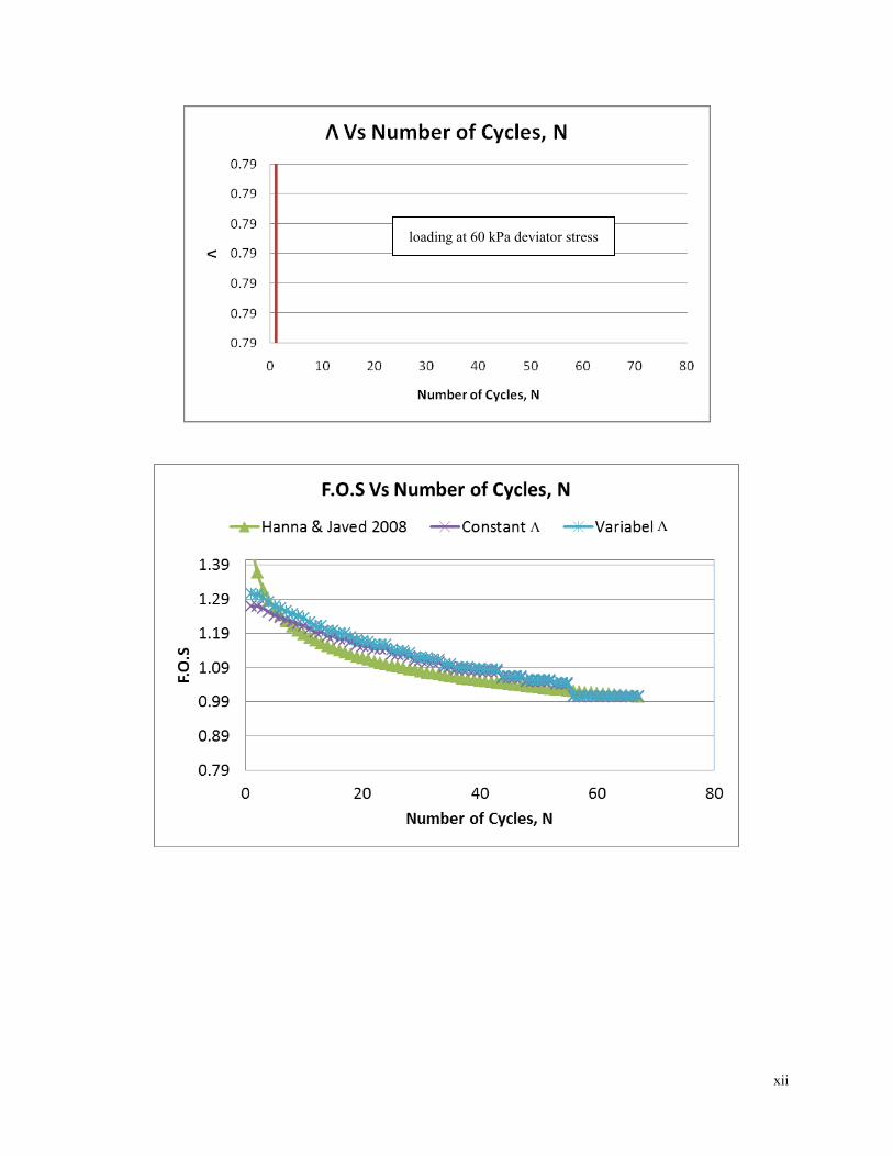
xii
loading at 60 kPa deviator stress
Ʌ
Ʌ