
Keystone summer school_2015_miguel_antonio_ldcompression_4-joined
219
Linked Data Semantic Technologies RDF Compression HDT Linked Data Compression Miguel A. Mart´ ınez-Prieto Antonio Fari˜ na Univ. of Valladolid (Spain) Univ. of A Coru˜ na (Spain) [email protected] [email protected] Keyword search over Big Data. – 1st KEYSTONE Training School –. July 22nd, 2015. Faculty of ICT, Malta. Miguel A. Mart´ ınez-Prieto & Antonio Fari˜ na Linked Data Compression 1/53
-
Upload
joel-azzopardi -
Category
Technology
-
view
479 -
download
0
Transcript of Keystone summer school_2015_miguel_antonio_ldcompression_4-joined

Linked DataSemantic Technologies
RDF CompressionHDT
Linked Data Compression
Miguel A. Martınez-Prieto Antonio FarinaUniv. of Valladolid (Spain) Univ. of A Coruna (Spain)
[email protected] [email protected]
Keyword search over Big Data.
– 1st KEYSTONE Training School –.July 22nd, 2015. Faculty of ICT, Malta.
Miguel A. Martınez-Prieto & Antonio Farina Linked Data Compression 1/53

Linked DataSemantic Technologies
RDF CompressionHDT
What is Linked Data?Linked Data PrinciplesLinked Open Data
Outline
1 Linked Data
2 Semantic Technologies
3 RDF Compression
4 HDT
Miguel A. Martınez-Prieto & Antonio Farina Linked Data Compression 2/53

Linked DataSemantic Technologies
RDF CompressionHDT
What is Linked Data?Linked Data PrinciplesLinked Open Data
– What is Linked Data? –
Linked Data
Linked Data is simply about using the Web to create typed linksbetween data from different sources [3].
Linked Data refers to a set of best practices for publishing andconnecting data on the Web.
These best practices have been adopted by an increasing number of data
providers, leading to the creation of a global data space:
Data are machine-readable.Data meaning is explicitly defined.Data are linked from/to external datasets.
The resulting Web of Data connects data from different domains:
Publications, movies, multimedia, government data, statistical data, etc.
Miguel A. Martınez-Prieto & Antonio Farina Linked Data Compression 3/53

Linked DataSemantic Technologies
RDF CompressionHDT
What is Linked Data?Linked Data PrinciplesLinked Open Data
What is Linked Data?
Miguel A. Martınez-Prieto & Antonio Farina Linked Data Compression 4/53

Linked DataSemantic Technologies
RDF CompressionHDT
What is Linked Data?Linked Data PrinciplesLinked Open Data
The Web... of Data
The emergence of the Web was an authentic revolution 15 years ago:Changed the way we consume information.Changed human relationships.Changed businesses....
Miguel A. Martınez-Prieto & Antonio Farina Linked Data Compression 5/53

Linked DataSemantic Technologies
RDF CompressionHDT
What is Linked Data?Linked Data PrinciplesLinked Open Data
The Web
The Web is a global space comprising linked HTML documents:Web pages are the atoms of the Web.Each page is univocally identified by their URL.
Miguel A. Martınez-Prieto & Antonio Farina Linked Data Compression 6/53

Linked DataSemantic Technologies
RDF CompressionHDT
What is Linked Data?Linked Data PrinciplesLinked Open Data
The Web
Where are (raw) data in the Web?Web pages “cook” raw data in a human-readable way.It is, probably, the main problem of the WWW.
Miguel A. Martınez-Prieto & Antonio Farina Linked Data Compression 7/53

Linked DataSemantic Technologies
RDF CompressionHDT
What is Linked Data?Linked Data PrinciplesLinked Open Data
The Web
- I was excited for the Keystone Training School and lookedfor information about this nice country.
- I wrote “malta” in a web search engine, and...
I found some relevant results for my query! :)
Miguel A. Martınez-Prieto & Antonio Farina Linked Data Compression 8/53

Linked DataSemantic Technologies
RDF CompressionHDT
What is Linked Data?Linked Data PrinciplesLinked Open Data
The Web
- I was excited for the Keystone Training School and lookedfor information about this nice country.
- I wrote “malta” in a web search engine, and...
But others seem a little strange to my (current) expectations... :(
Miguel A. Martınez-Prieto & Antonio Farina Linked Data Compression 9/53

Linked DataSemantic Technologies
RDF CompressionHDT
What is Linked Data?Linked Data PrinciplesLinked Open Data
The Web... of Data
Raw data are hidden among web pages contents:
In general, data are written in HTML paragraphs.In the best case, they are structured in the form of HTML tables orpublished as additional documents (CSV, XML...)
Anyway, HTML is not enough expressive to describe and link individual
data entities in the Web:
HTML-based descriptions lose semantics and structure from the rawdata.
This fact makes very difficult automatic data processing in the Web.
Miguel A. Martınez-Prieto & Antonio Farina Linked Data Compression 10/53

Linked DataSemantic Technologies
RDF CompressionHDT
What is Linked Data?Linked Data PrinciplesLinked Open Data
The Web... of Data
The Web of Data [8] converts raw data into first-class citizens of the
Web...
Data entities are the atoms of the Web of Data.Each entity has its own identity.
...and uses existing infrastructure:
It uses HTTP as communication protocol.Entities are named using URIs.
The Web of Data is a cloud of data-to-data hyperlinks [5]:
These are labelled hyperlinks in contrast to the “plain” ones usedin the Web.Thus, hyperlinks also provide semantics to data descriptions.
Miguel A. Martınez-Prieto & Antonio Farina Linked Data Compression 11/53

Linked DataSemantic Technologies
RDF CompressionHDT
What is Linked Data?Linked Data PrinciplesLinked Open Data
The Web... of Data
Linked Data builds a Web of Data using the Internet infrastructure:Data providers can publish their raw data in a standardized way.These data can be interconnected using labelled hyperlinks.The resulting cloud of data can be navigated using specific querylanguages.
Linked Data achievements:
Knowledge from different fields can be easily integrated and universallyshared.Automatic processes can exploit these knowledge to build innovativesoftware systems.
Semantic Search Engine
For instance, a semantic search engine would allow us for only retrieving entities whichdescribe “malta” as a country but not as a cereal.
Miguel A. Martınez-Prieto & Antonio Farina Linked Data Compression 12/53

Linked DataSemantic Technologies
RDF CompressionHDT
What is Linked Data?Linked Data PrinciplesLinked Open Data
– Linked Data Principles –
Tim Berners-Lee [2] suggests four basic principles for Linked Data:
1 Use URIs as names for things.
2 Use HTTP URIs so that people can look up those names.
3 When someone looks up a URI, provide useful information, using thestandards (RDF, SPARQL).
4 Include links to other URIs, so that they can discover more things.
Miguel A. Martınez-Prieto & Antonio Farina Linked Data Compression 13/53

Linked DataSemantic Technologies
RDF CompressionHDT
What is Linked Data?Linked Data PrinciplesLinked Open Data
1. URIs as names
What is his name?
For humans, his name is Clint Eastwood...
... but http://dataweb.infor.uva.es/movies/people/Clint Eastwood is abetter name for machines.
The use of URIs enables real-world entities (or their relationships withother entities) to be identifed at universal scale.
This principle ensures any class of data has its own identity in the globalspace of the Web of Data.
Miguel A. Martınez-Prieto & Antonio Farina Linked Data Compression 14/53

Linked DataSemantic Technologies
RDF CompressionHDT
What is Linked Data?Linked Data PrinciplesLinked Open Data
2. HTTP URIs
All entities must be described using dereferenceable URIs:
These URIs are accesible via HTTP.
This principle exploits HTTP features to retrieve all data related to agiven URI.
Miguel A. Martınez-Prieto & Antonio Farina Linked Data Compression 15/53

Linked DataSemantic Technologies
RDF CompressionHDT
What is Linked Data?Linked Data PrinciplesLinked Open Data
3. Standards
This principle states that allstakeholders “must speak the samelanguages” for effectiveunderstanding.
RDF [10] provides a simple logicalmodel for data description.
SPARQL [12] describes a specificlanguage for querying RDF data.
Serialization formats, ontologylanguages, etc.
Miguel A. Martınez-Prieto & Antonio Farina Linked Data Compression 16/53

Linked DataSemantic Technologies
RDF CompressionHDT
What is Linked Data?Linked Data PrinciplesLinked Open Data
4. Linking URIs
This principle materializes the aim of data integration in Linked Data:
Linking two URIs establishes a particular connection between two existingentities.
Linking URIs
http://dataweb.infor.uva.es/movies/people/Clint Eastwood names the entity whichdescribes “Clint Eastwood”.
http://dataweb.infor.uva.es/movies/film/Mystic River names the entity which describesthe movie “Mystic River”.
An hyperlink between these two URIs state that the entity “Clint Eastwood” is
related to the entity “Mystic River”... how?
The labelled link provides a semantic relationship between entities.In this case, http://dataweb.infor.uva.es/movies/property/director tags the“director” relationship between “Clint Eastwood” and “Mystic River”.
Miguel A. Martınez-Prieto & Antonio Farina Linked Data Compression 17/53

Linked DataSemantic Technologies
RDF CompressionHDT
What is Linked Data?Linked Data PrinciplesLinked Open Data
– Linked Open Data –
The Linked Open Data (LOD) project1 promotes Linked Data to be
published as Open Data:
LOD is released under an open license which does not impede its reuse forfree [2].
LOD is the highest-level in the 5-star scheme2 for Open Data publication.
? The dataset is available on the Web under an open license.
?? The dataset is available as structured data.
? ? ? The dataset is encoded using a non-propietary format.
? ? ?? The dataset names entities using URIs.
? ? ? ? ? The dataset is linked to other datasets.
1http://linkeddata.org/; http://5stardata.info/
Miguel A. Martınez-Prieto & Antonio Farina Linked Data Compression 18/53

Linked DataSemantic Technologies
RDF CompressionHDT
What is Linked Data?Linked Data PrinciplesLinked Open Data
LOD (2007-2011)
Miguel A. Martınez-Prieto & Antonio Farina Linked Data Compression 19/53

Linked DataSemantic Technologies
RDF CompressionHDT
What is Linked Data?Linked Data PrinciplesLinked Open Data
LOD (2014)
Miguel A. Martınez-Prieto & Antonio Farina Linked Data Compression 20/53

Linked DataSemantic Technologies
RDF CompressionHDT
What is Linked Data?Linked Data PrinciplesLinked Open Data
LOD (2014)
Miguel A. Martınez-Prieto & Antonio Farina Linked Data Compression 21/53

Linked DataSemantic Technologies
RDF CompressionHDT
What is Linked Data?Linked Data PrinciplesLinked Open Data
Current Statistics (July, 2015)
9,960 datasets are openly available2:
90 billion statements from 3,308 datasets.6,639 datasets could not be crawled for different reasons.
LOD Laundromat4 provides access to more tha 38 billion statementsfrom 650K “cleaned” datasets.
DBpedia 2014 contains more than 3 billion statements:538 million statements from English Wikipedia.2.46 billion statements from other language editions.50 million statements linking to external datasets.
More and more datasets are released and these are getting bigger:
The largest ones are in the order of hundreds of GB.
2http://stats.lod2.eu/; http://lodlaundromat.org/
Miguel A. Martınez-Prieto & Antonio Farina Linked Data Compression 22/53

Linked DataSemantic Technologies
RDF CompressionHDT
OverviewRDFSPARQL
Outline
1 Linked Data
2 Semantic Technologies
3 RDF Compression
4 HDT
Miguel A. Martınez-Prieto & Antonio Farina Linked Data Compression 23/53

Linked DataSemantic Technologies
RDF CompressionHDT
OverviewRDFSPARQL
– Overview –
Semantic Technologies (in middle
layers) exploit features from the Web
infrastructure (low layers):
RDF is used for resourcedescription.RDFS is used for describingsemantic vocabularies.OWL extends RDFS and is usedfor building ontologies.SPARQL is the query language forRDF data.RIF is used for describing rules.
Miguel A. Martınez-Prieto & Antonio Farina Linked Data Compression 24/53

Linked DataSemantic Technologies
RDF CompressionHDT
OverviewRDFSPARQL
RDF & SPARQL
RDF & SPARQL are the most relevant technologies for our current aims:
Both standards are based on labelled directed graph features.
Miguel A. Martınez-Prieto & Antonio Farina Linked Data Compression 25/53

Linked DataSemantic Technologies
RDF CompressionHDT
OverviewRDFSPARQL
– RDF –
http : //dataweb.infor.uva.es/movies/people/Clint Eastwoodhttp : //dataweb.infor.uva.es/movies/property/name′Clint Eastwood′
http : //dataweb.infor.uva.es/movies/film/Mystic Riverhttp : //dataweb.infor.uva.es/movies/property/title′Mystic River′
http : //dataweb.infor.uva.es/movies/people/Clint Eastwoodhttp : //dataweb.infor.uva.es/movies/property/directorhttp : //dataweb.infor.uva.es/movies/film/Mystic River
RDF [10] is a framework for describing resources of any class:
People, movies, cities, proteins, statistical data...
Resources are described in the form of triples:
Subject: the resource being described.Predicate: a property of that resource.Object: the value for the corresponding property.
Miguel A. Martınez-Prieto & Antonio Farina Linked Data Compression 26/53

Linked DataSemantic Technologies
RDF CompressionHDT
OverviewRDFSPARQL
RDF Triples
http : //dataweb.infor.uva.es/movies/people/Clint Eastwoodhttp : //dataweb.infor.uva.es/movies/property/name′Clint Eastwood′
http : //dataweb.infor.uva.es/movies/film/Mystic Riverhttp : //dataweb.infor.uva.es/movies/property/title′Mystic River′
http : //dataweb.infor.uva.es/movies/people/Clint Eastwoodhttp : //dataweb.infor.uva.es/movies/property/directorhttp : //dataweb.infor.uva.es/movies/film/Mystic River
An RDF triple is a labelled directed subgraph in which subject and object
nodes are linked by a particular (predicate) edge:
The subject node contains the URI which names the resource.The predicate edge labels the relationship using a URI whose semantics isdescribed by any vocabulary/ontology.The object node may contain a URI or a (string) Literal value.
RDF links (between entities) also take the form of RDF triples.
Miguel A. Martınez-Prieto & Antonio Farina Linked Data Compression 27/53

Linked DataSemantic Technologies
RDF CompressionHDT
OverviewRDFSPARQL
RDF Triples
Miguel A. Martınez-Prieto & Antonio Farina Linked Data Compression 28/53

Linked DataSemantic Technologies
RDF CompressionHDT
OverviewRDFSPARQL
RDF Triples
Miguel A. Martınez-Prieto & Antonio Farina Linked Data Compression 29/53

Linked DataSemantic Technologies
RDF CompressionHDT
OverviewRDFSPARQL
RDF Triples
Miguel A. Martınez-Prieto & Antonio Farina Linked Data Compression 30/53
Linked DataSemantic Technologies
RDF CompressionHDT
OverviewRDFSPARQL
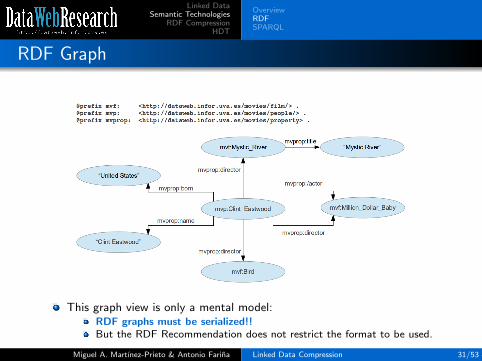
RDF Graph
This graph view is only a mental model:RDF graphs must be serialized!!But the RDF Recommendation does not restrict the format to be used.
Miguel A. Martınez-Prieto & Antonio Farina Linked Data Compression 31/53

Linked DataSemantic Technologies
RDF CompressionHDT
OverviewRDFSPARQL
RDF Serialization Formats
Traditional plain formats are commonly used:
RDF/XML, NTriples, Turtle...
These formats are very verbose in practice:
Data are serialized in a (more or less) human-readable way.
Large RDF files are finally compressed using gzip or bzip2.
Miguel A. Martınez-Prieto & Antonio Farina Linked Data Compression 32/53

Linked DataSemantic Technologies
RDF CompressionHDT
OverviewRDFSPARQL
– SPARQL –
SPARQL [12] is a query language for RDF.
It is based on graph pattern matching:
Triple patterns are RDF triples in which subject, predicate and object maybe variable.
SPARQL supports more complex queries: joins, unions, filters...
Miguel A. Martınez-Prieto & Antonio Farina Linked Data Compression 33/53

Linked DataSemantic Technologies
RDF CompressionHDT
OverviewRDFSPARQL
SPARQL Resolution
Miguel A. Martınez-Prieto & Antonio Farina Linked Data Compression 34/53

Linked DataSemantic Technologies
RDF CompressionHDT
OverviewRDFSPARQL
SPARQL Resolution
Miguel A. Martınez-Prieto & Antonio Farina Linked Data Compression 35/53

Linked DataSemantic Technologies
RDF CompressionHDT
OverviewRDFSPARQL
SPARQL Resolution
Miguel A. Martınez-Prieto & Antonio Farina Linked Data Compression 36/53
Linked DataSemantic Technologies
RDF CompressionHDT
Semantic CompressionSymbolic CompressionSyntactic Compression
Outline
1 Linked Data
2 Semantic Technologies
3 RDF Compression
4 HDT
Miguel A. Martınez-Prieto & Antonio Farina Linked Data Compression 37/53

Linked DataSemantic Technologies
RDF CompressionHDT
Semantic CompressionSymbolic CompressionSyntactic Compression
What is the problem?
RDF excels at logical level:Structured and semi-structured data can be described using RDF triples.Entities are also linked in the form of RDF triples.
But it is a source of redundancy at physical levelSerialization formats are highly verbose.RDF data are redundant at three levels: semantic, symbolic, andsyntactic.
Miguel A. Martınez-Prieto & Antonio Farina Linked Data Compression 38/53

Linked DataSemantic Technologies
RDF CompressionHDT
Semantic CompressionSymbolic CompressionSyntactic Compression
– Semantic Compression –
Semantic redundancy occurs when the same meaning can be conveyedusing less triples.
http : //dataweb.infor.uva.es/movies/property/namehttp : //www.w3.org/2000/01/rdf − schema#domainhttp : //dataweb.infor.uva.es/movies/classes/person
http : //dataweb.infor.uva.es/movies/people/Clint Eastwoodhttp : //dataweb.infor.uva.es/movies/property/name′Clint Eastwood′
http : //dataweb.infor.uva.es/movies/people/Clint Eastwoodhttp : //www.w3.org/1999/02/22 − rdf − syntax − ns#typehttp : //dataweb.infor.uva.es/movies/classes/person
The third triple is redundant because the first one state that the URIhttp://dataweb.infor.uva.es/movies/people/Clint Eastwood describes an entity in thedomain of http://dataweb.infor.uva.es/movies/classes/person.
Miguel A. Martınez-Prieto & Antonio Farina Linked Data Compression 39/53

Linked DataSemantic Technologies
RDF CompressionHDT
Semantic CompressionSymbolic CompressionSyntactic Compression
Semantic Compression
Semantic compressors perform at logical level:
Detect redundant triples and remove them from the original dataset.
Semantic compressors [9, 11, 13] are not so effective by themselves...
... but may be combined with symbolic and syntactic compressors!
Miguel A. Martınez-Prieto & Antonio Farina Linked Data Compression 40/53

Linked DataSemantic Technologies
RDF CompressionHDT
Semantic CompressionSymbolic CompressionSyntactic Compression
– Symbolic Compression –
Symbolic redundancy is due to symbol repetitions in triples:
This is the “traditional” source of redundancy removed by universalcompressors.
Symbolic redundancy in RDF is mainly due to URIs:
URIs tend to be very large strings which share long prefixes.
http://dataweb.infor.uva.es/movies/film/Bird
http://dataweb.infor.uva.es/movies/film/Million Dollar Baby
http://dataweb.infor.uva.es/movies/film/Mystic River
http://dataweb.infor.uva.es/movies/people/Clint Eastwood
...
... but literals also contibute to this redundancy.
Miguel A. Martınez-Prieto & Antonio Farina Linked Data Compression 41/53

Linked DataSemantic Technologies
RDF CompressionHDT
Semantic CompressionSymbolic CompressionSyntactic Compression
Symbolic Compression
The most prominent RDF compressors remove symbolic redundancy:
All different URIs/literals are indexed in a string dictionary.Each string is identified by a unique integer ID.
- Triples are rewritten by replacing strings by their corresponding IDs.
Symbolic is, in general, the most important redundancy in RDF and has(many) room for optimization.
Miguel A. Martınez-Prieto & Antonio Farina Linked Data Compression 42/53

Linked DataSemantic Technologies
RDF CompressionHDT
Semantic CompressionSymbolic CompressionSyntactic Compression
– Syntactic Compression –
Syntactic redundancy depends on the RDF graph serialization:
For instance, a serialized subset of n triples (which describes the sameresource) writes n times the subject value. It can be abbr.
... and also on the underlying graph structure:
For instance, resources of the same classes are described using (almost)the same sub-graph structure.
Syntactic compression also has (many) room for optimization.
Miguel A. Martınez-Prieto & Antonio Farina Linked Data Compression 43/53

Linked DataSemantic Technologies
RDF CompressionHDT
Semantic CompressionSymbolic CompressionSyntactic Compression
Syntactic Compression
HDT [7], k2-triples [1], or RDFCSA [4] are syntactic compressors
reporting good numbers:
They are combined with symbolic compression.In practice, they compress RDF triples in the form of ID triples.
Semantic compressors such as SSP [11] also remove symbolic andsyntactic redundancy.
Miguel A. Martınez-Prieto & Antonio Farina Linked Data Compression 44/53

Linked DataSemantic Technologies
RDF CompressionHDT
BasicsComponentsConclusions
Outline
1 Linked Data
2 Semantic Technologies
3 RDF Compression
4 HDT
Miguel A. Martınez-Prieto & Antonio Farina Linked Data Compression 45/53

Linked DataSemantic Technologies
RDF CompressionHDT
BasicsComponentsConclusions
– What is HDT? –
HDT was the first binary serialization format for RDF:It was acknowledged as W3C Member Submission [6] in 2011.
It exploits symbolic and syntactic redundancy:It reduces up to 15 times the space used by traditional formats [7].
HDT is a core building block in some Linked Data applications:It reports good compression numbers, but also provides efficient dataretrieval.
Miguel A. Martınez-Prieto & Antonio Farina Linked Data Compression 46/53

Linked DataSemantic Technologies
RDF CompressionHDT
BasicsComponentsConclusions
– Components –
HDT encodes RDF data into three components:The Header (H) comprises descriptive metadata.
The Dictionary (D) maps different strings (from nodes and edges) to IDs:It manages four independent mappings: subjects-objects, subjects, objects, andpredicates.
The Triples (T) component encodes the inner structure as a graph of IDs.
Miguel A. Martınez-Prieto & Antonio Farina Linked Data Compression 47/53

Linked DataSemantic Technologies
RDF CompressionHDT
BasicsComponentsConclusions
HDT Components
The Dictionary is encoded using specific compression techniques for stringdictionaries.
Triple IDs are organized into a forest of trees (one per different subject)...
...which is encoded using two bitsequences and two ID sequences.
Miguel A. Martınez-Prieto & Antonio Farina Linked Data Compression 48/53

Linked DataSemantic Technologies
RDF CompressionHDT
BasicsComponentsConclusions
– Conclusions –
HDT integrates RDF serialization and compression into a practical
format:
HDT saves space storage and enables efficient data parsing/retrievalusing bit operations.
Symbolic rendundancy is addressed by the Dictionary component:
The collection of strings (in the dictionary) has high symbolicredundancy...The own dictionary is highly compressible!
Syntactic rendundancy is removed by the Triples component:
HDT triples is a straightforward compressor.Their effectiveness can be improved using optimized graph compressiontechniques.
Miguel A. Martınez-Prieto & Antonio Farina Linked Data Compression 49/53

Linked DataSemantic Technologies
RDF CompressionHDT
BasicsComponentsConclusions
Bibliography I
[1] Sandra Alvarez-Garcıa, Nieves Brisaboa, Javier D. Fernandez, Miguel A. Martınez-Prieto, and GonzaloNavarro.Compressed Vertical Partitioning for Efficient RDF Management.Knowledge and Information Systems (KAIS), 44(2):439–474, 2015.
[2] Tim Berners-Lee.Linked Data, 2006.http://www.w3.org/DesignIssues/LinkedData.html.
[3] Christian Bizer, Tom Heath, and Tim Berners-Lee.Linked Data - The Story So Far.International Journal of Semantic Web and Information Systems, 5(3):1–22, 2009.
[4] Nieves Brisaboa, Ana Cerdeira, Antonio Farina, and Gonzalo Navarro.A Compact RDF Store using Suffix Arrays.In Proceedings of SPIRE, 2015.To appear.
[5] Javier D. Fernandez, Mario Arias, Miguel A. Martınez-Prieto, and Claudio Gutierrez.Management of Big Semantic Data.In Big Data Computing, chapter 4. Taylor and Francis/CRC, 2013.
[6] Javier D. Fernandez, Miguel A. Martınez-Prieto, Claudio Gutierrez, and Axel Polleres.Binary RDF Representation for Publication and Exchange.W3C Member Submission, 2011.www.w3.org/Submission/HDT/.
Miguel A. Martınez-Prieto & Antonio Farina Linked Data Compression 50/53

Linked DataSemantic Technologies
RDF CompressionHDT
BasicsComponentsConclusions
Bibliography II
[7] Javier D. Fernandez, Miguel A. Martınez-Prieto, Claudio Gutierrez, Axel Polleres, and Mario Arias.Binary RDF Representation for Publication and Exchange.Journal of Web Semantics, 19:22–41, 2013.
[8] Tom Heath and Christian Bizer.Linked Data: Evolving the Web into a Global Data Space.Morgan & Claypool, 1 edition, 2011.http://linkeddatabook.com/.
[9] Amit K. Joshi, Pascal Hitzler, and Guozhu Dong.Logical Linked Data Compression.In Proceedings of ESWC, pages 170–184, 2013.
[10] Frank Manola and Eric Miller.RDF Primer.W3C Recommendation, 2004.www.w3.org/TR/rdf-primer/.
[11] Jeff Z. Pan, Jose Manuel Gomez-Perez, Yuan Ren, Honghan Wu, and Man Zhu.SSP: Compressing RDF data by Summarisation, Serialisation and Predictive Encoding.Technical report, 2014.Available at http://www.kdrive-project.eu/wp-content/uploads/2014/06/WP3-TR2-2014 SSP.pdf.
[12] Eric Prud’hommeaux and Andy Seaborne.SPARQL Query Language for RDF.W3C Recommendation, 2008.http://www.w3.org/TR/rdf-sparql-query/.
Miguel A. Martınez-Prieto & Antonio Farina Linked Data Compression 51/53

Linked DataSemantic Technologies
RDF CompressionHDT
BasicsComponentsConclusions
Bibliography III
[13] Gayathri V. and P. Sreenivasa Kumar.Horn-Rule based Compression Technique for RDF Data.In Proceedings of SAC, pages 396–401, 2015.
Miguel A. Martınez-Prieto & Antonio Farina Linked Data Compression 52/53

Linked DataSemantic Technologies
RDF CompressionHDT
BasicsComponentsConclusions
This presentation has been made available only for learning/teaching purposes.The pictures used in the slides may be owned by other parties, so their property is exclusively of their authors.
Miguel A. Martınez-Prieto & Antonio Farina Linked Data Compression 53/53

Onto some basics of: compression, Compact Data Structures, and
indexing
1st KEYSTONE Training School July 22th, 2015. Faculty of ICT, Malta
Antonio Fariña
Miguel A Martínez Prieto

Outline
Introduction Basic compression Sequences
Bit sequences Integer sequences
A brief Review about Indexing

• Disks are cheap !! But they are also slow! – Compression can help more data to fit in main memory. (access to memory is around 106 times faster than HDD)
• CPU speed is increasing faster – We can trade processing time (needed to uncompress
data) by space.
Introduction Why compression?

• Compression does not only reduce space! – I/O access on disks and networks – Processing time* (less data has to be processed)
• … If appropriate methods are used – For example: Allowing handling data compressed all the time.
Introduction Why compression?
Text collection (100%)
Doc 1 Doc 2 Doc 3 Doc n Compressed Text collection (30%)
Doc 1 Doc 2 Doc 3 Doc n
Compressed Text collection (20%) P7zip, others
Doc 1 Doc 2 Doc 3 Doc n
Let’s search for “Malta"

• Indexing permits sublinear search time
Introduction Why indexing?
Text collection (100%)
Doc 1 Doc 2 Doc 3 Doc n Compressed Text collection (30%)
Doc 1 Doc 2 Doc 3 Doc n
Let’s search for “Malta"
term 1 …
Malta …
term n
(> 5-30%) Index

• Self-indexes: – sublinear search time – Text implicitly kept
Introduction Why Compact Data Structures?
Text collection
Doc 1 Doc 2 Doc 3 Doc n
Let’s search for “Malta"
term 1 …
Malta …
term n
(> 5-30%) Index
0 0 0 0 1 1
0 1
0 1 0 1 0 0
1
0
Self-index (WT, WCSA,…)
term 1 …
Malta …
term n
Outline
Introduction Basic compression Sequences
Bit sequences Integer sequences
A brief Review about Indexing

Basic Compression
• A compressor could use as a source alphabet: – A fixed number of symbols (statistical compressors)
• 1 char, 1 word – A variable number of symbols (dictionary-based compressors)
• 1st occ of ‘a’ encoded alone, 2nd occ encoded with next one ‘ax’
• Codes are built using symbols of an target alphabet: – Fixed length codes (1 bit, 10 bits, 1 byte, 2 bytes, …) – Variable length codes (1,2,3,4 bits/bytes …)
• Classification (fixed-to-variable, variable-to-fixed,…)
Modeling & Coding
-- statistical Input alphabet
dictionary var2var
Target alphabet
fixed var
fixed var

Basic Compression
• Taxonomy – Dictionary based (gzip, compress, p7zip… ) – Grammar based (BPE, Repair) – Statistical compressors (Huffman, arithmetic, PPM,… )
• Statistical compressors – Gather the frequencies of the source symbols. – Assign shorter codewords to the most frequent symbols.
Obtain compression
Main families of compressors

Basic Compression
• How do they achieve compression – Assign fixed-length codewords to variable length symbols (text
substrings) – The longer the replaced substring the better compression
• Well-known representatives: Lempel-Ziv family
– LZ77 (1977): GZIP, PKZIP, ARJ, P7zip – LZ89 (1978)
• LZW (1984): Compress, GIF images
Dictionary-based compressors

Basic Compression
• Starts with an initial dictionary D (contains symbols in Σ) • For a given position of the text.
– while D contains w, reads prefix w=w0 w1 w2 … – If w0 …wk wk+1 is not in D (w0 …wk does!)
• output (i = entryPos(w0 …wk)) (Note: codeword = log2 (|D|)) • Add w0 …wk wk+1 to D • Continue from wk+1 on (included)
• Dictionary has limited length? Policies: LRU, truncate& go, …
LZW
EXA
MPL
E

Basic Compression
• Replaces pairs of symbols by a new one, until no pair repeats twice – Adds a rule to a Dictionary.
Grammar Based – BPE - Repair
A B C D E A B D E F D E D E F A B E C D
A B C G A B G F G G F A B E C D
H C G H G F G G F H E C D
H C G H I G I H E C D
DE G
AB H
GF I
Source sequence
Dictionary of Rules
Final Repair Sequence

Basic Compression
• Assign shorter codewords to the most frequent symbols – Must gather symbol frequencies for each symbol c in Σ. – Compression is lower bounded by the (zero-order) empirical
entropy of the sequence (S).
• Most representative method: Huffman coding
Statistical Compressors
n= num of symbols
nc= occs of symbol c
H0(S) <= log (|Σ|) n H0(S) = lower bound of the size of S compressed with a zero-order compressor

Basic Compression
• Optimal prefix free coding – No codeword is a prefix of one another.
• Decoding requires no look-ahead!
– Asymptotically optimal: |Huffman(S)| <= n(H0(S)+1)
• Typically using bit-wise codewords – Yet D-ary Huffman variants exist (D=256 byte-wise)
• Builds a Huffman tree to generate codewords
Statistical Compressors: Huffman coding

Basic Compression
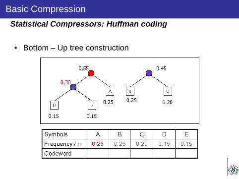
• Sort symbols by frequency: S=ADBAAAABBBBCCCCDDEEE
Statistical Compressors: Huffman coding

Basic Compression
• Bottom – Up tree construction
Statistical Compressors: Huffman coding

Basic Compression
• Bottom – Up tree construction
Statistical Compressors: Huffman coding

Basic Compression
• Bottom – Up tree construction
Statistical Compressors: Huffman coding
Basic Compression
• Bottom – Up tree construction
Statistical Compressors: Huffman coding

Basic Compression
• Bottom – Up tree construction
Statistical Compressors: Huffman coding

Basic Compression
• Branch labeling
Statistical Compressors: Huffman coding

Basic Compression
• Code assignment
Statistical Compressors: Huffman coding

Basic Compression
• Compression of sequence S= ADB…
• ADB… 01 000 10 …
Statistical Compressors: Huffman coding

Basic Compression
• Given S= mississipii$, BWT(S) is obtained by: (1) creating a Matrix M with all circular permutations of S$, (2) sorting the rows of M, and (3) taking the last column.
Burrows-Wheeler Transform (BWT)
mississippi$
$mississippi
i$mississipp
pi$mississip
ppi$mississi
ippi$mississ
sippi$missis
ssippi$missi
issippi$miss
sissippi$mis
ssissippi$mi
ississippi$m
$mississippi
i$mississipp
ippi$mississ
issippi$miss
ississippi$m
mississippi$
pi$mississip
ppi$mississi
sippi$missis
sissippi$mis
ssippi$missi
ssissippi$mi
sort
L = BWT(S) F

Basic Compression
• Given L=BWT(S), we can recover S=BWT-1(L)
Burrows-Wheeler Transform: reversible (BWT -1)
$mississippi
i$mississipp
ippi$mississ
issippi$miss
ississippi$m
mississippi$
pi$mississip
ppi$mississi
sippi$missis
sissippi$mis
ssippi$missi
ssissippi$mi
L F
1
2
3
4
5
6
7
8
9
10
11
12
2
7
9
10
6
1
8
3
11
12
4
5
LF
Steps: 1. Sort L to obtain F 2. Build LF mapping so that
If L[i]=‘c’, and k= the number of times ‘c’ occurs in L[1..i], and j=position in F of the kth occurrence of ‘c’ Then set LF[i]=j
Example: L[7] = ‘p’, it is the 2nd ‘p’ in L LF[7] = 8 which is the 2nd occ of ‘p’ in F
3. Recover the source sequence S in n steps:
Initially p=l=6 (position of $ in L); i=0; n=12; In each step: S[n-i] = L[p]; p = LF[p];
i = i+1;
-
-
-
-
-
-
-
-
-
-
-
$
S

Basic Compression
• Given L=BWT(S), we can recover S=BWT-1(L)
Burrows-Wheeler Transform: reversible (BWT -1)
$mississippi
i$mississipp
ippi$mississ
issippi$miss
ississippi$m
mississippi$
pi$mississip
ppi$mississi
sippi$missis
sissippi$mis
ssippi$missi
ssissippi$mi
L F
1
2
3
4
5
6
7
8
9
10
11
12
2
7
9
10
6
1
8
3
11
12
4
5
LF
Steps: 1. Sort L to obtain F 2. Build LF mapping so that
If L[i]=‘c’, and k= the number of times ‘c’ occurs in L[1..i], and j=position in F of the kth occurrence of ‘c’ Then set LF[i]=j
Example: L[7] = ‘p’, it is the 2nd ‘p’ in L LF[7] = 8 which is the 2nd occ of ‘p’ in F
3. Recover the source sequence S in n steps:
Initially p=l=6 (position of $ in L); i=0; n=12; Step i=0: S[n-i] = L[p]; S[12]=‘$’ p = LF[p]; p = 1
i = i+1; i=1
-
-
-
-
-
-
-
-
-
-
-
$
S

Basic Compression
• Given L=BWT(S), we can recover S=BWT-1(L)
Burrows-Wheeler Transform: reversible (BWT -1)
$mississippi
i$mississipp
ippi$mississ
issippi$miss
ississippi$m
mississippi$
pi$mississip
ppi$mississi
sippi$missis
sissippi$mis
ssippi$missi
ssissippi$mi
L F
1
2
3
4
5
6
7
8
9
10
11
12
2
7
9
10
6
1
8
3
11
12
4
5
LF
Steps: 1. Sort L to obtain F 2. Build LF mapping so that
If L[i]=‘c’, and k= the number of times ‘c’ occurs in L[1..i], and j=position in F of the kth occurrence of ‘c’ Then set LF[i]=j
Example: L[7] = ‘p’, it is the 2nd ‘p’ in L LF[7] = 8 which is the 2nd occ of ‘p’ in F
3. Recover the source sequence S in n steps:
Initially p=l=6 (position of $ in L); i=0; n=12; Step i=1: S[n-i] = L[p]; S[11]=‘i’ p = LF[p]; p = 2
i = i+1; i=2
-
-
-
-
-
-
-
-
-
-
i
$
S

Basic Compression
• Given L=BWT(S), we can recover S=BWT-1(L)
Burrows-Wheeler Transform: reversible (BWT -1)
$mississippi
i$mississipp
ippi$mississ
issippi$miss
ississippi$m
mississippi$
pi$mississip
ppi$mississi
sippi$missis
sissippi$mis
ssippi$missi
ssissippi$mi
L F
1
2
3
4
5
6
7
8
9
10
11
12
2
7
9
10
6
1
8
3
11
12
4
5
LF
Steps: 1. Sort L to obtain F 2. Build LF mapping so that
If L[i]=‘c’, and k= the number of times ‘c’ occurs in L[1..i], and j=position in F of the kth occurrence of ‘c’ Then set LF[i]=j
Example: L[7] = ‘p’, it is the 2nd ‘p’ in L LF[7] = 8 which is the 2nd occ of ‘p’ in F
3. Recover the source sequence S in n steps:
Initially p=l=6 (position of $ in L); i=0; n=12; Step i=1: S[n-i] = L[p]; S[11]=‘i’ p = LF[p]; p = 2
i = i+1; i=2
m
i
s
s
i
s
s
i
p
i
i
$
S

Basic Compression
• BWT. Many similar symbols appear adjacent • MTF.
– Output the position o the current symbol within Σ ‘ – Keep the alphabet Σ ‘= {a,b,c,d,e,… } sorted so that the last used
symbol is moved to the begining of Σ ‘ . • RLE.
– If a value (0) appears several times (000000 6 times) – replace it by a pair <value,times> <0,6>
• Huffman stage.
Bzip2: Burrows-Wheeler Transform (BWT)
Why does it work? In a text it is likely that “he” is preceeded by “t”, “ssisii” by “i”, …

Outline
Introduction Basic compression Sequences
Bit sequences Integer sequences
A brief Review about Indexing

Sequences
• Given a Sequence of – n integers – m = maximum value
• We can representing it with n ⌈log2(m+1)⌉ bits
– 16 symbols x3 bits per symbol = 48 bits array of 2 32-bit ints – Direct access (access to an integer + bit operations)
Plain Representation of Data
4 1 4 4 4 4 1 4 2 4 1 1 2 3 4 4 1 2 3 4 5 6 7 8 9 10 11 12 13 14 15 16
100 010 100 100 100 100 001 100 010 100 001 001 010 011 100 100 1 2 3 4 5 6 7 8 9 10 11 12 13 14 15 16

Sequences
• Is it compressible?
• Ho(S) = 1.59 (bits per symbol)
• Huffman: 1.62 bits per symbol
26 bits: No direct access! (but we could add sampling)
Compresed Representation of Data (H0)
Symbol 4 1 2 3
Occurrences (nc) 9 4 2 1
0 1 16
7
1 4 3
0
1
2
0
1
2 3 1 4
9
4 1 4 4 4 4 1 4 2 4 1 1 2 3 4 4 1 2 3 4 5 6 7 8 9 10 11 12 13 14 15 16
1 01 000 001 1 1 1 1 01 1 000 1 01 01 1 1 1 5 10 15 20 25

Sequences
• Operations of interest:
– Access(i) : Value of the ith symbol – Ranks(i) : Number of occs of symbol s up to position i (count) – Selects (i) : Where the ith occ of symbol s? (locate)
Summary: Plain/compressed acess/rank/select ()
4 1 4 4 4 4 1 4 2 4 1 1 2 3 4 4 1 2 3 4 5 6 7 8 9 10 11 12 13 14 15 16
100 010 100 100 100 100 001 100 010 100 001 001 010 011 100 100 1 4 5 10 13 16 19 22 25 28 31 34 37 40 43 46
1 01 000 001 1 1 1 1 01 1 000 1 01 01 1 1 1 5 10 15 20 25

Outline
Introduction Basic compression Sequences
Bit sequences Integer sequences
A brief Review about Indexing

Bit Sequences
Rank1(6) = 3 Rank0(10) = 5
Access/rank/select on bitmaps
0 1 0 0 1 1 0 1 1 0 0 0 0 0 0 1 0 0 0 0 01 2 3 4 5 6 7 8 9 10 11 12 13 14 15 16 17 18 19 20 21
B=
select0(10) =15
access (19) = 0

Bit Sequences
• Bitmaps a basic part of most Compact Data Structures
• Example: (We will see it later in the CSA)
S: AAABBCCCCCCCCDDDEEEEEEEEEEFG n log σ bits
B: 1001010000000100100000000011 n bits
D: ABCDEFG σ log σ bits
– Saves space: – Fast access/rank/select is of interest !!
• Where is the 2nd C? • How many Cs up to position k?
Applications

Bit Sequences
• Jacobson, Clark, Munro – Variant by Fariña et al.
• Assuming 32 bit machine-word
• Step 1: Split de Bitmap into superblocks of 256 bits, and store de number of 1s up to positions 1+256k – O(1) time to superblock. Space: n/256 superblock and 1 int each
Reaching O(1) Rank y o(n) bits of extra space
0 1 0 ... 11 2 3 256
35 bits set to 1
1 ... 1257 512
27 bits set to 1
350
1 2
Ds = 62
3
0 ... 1513 768
45 bits set to 1
...
97
3
...
Bit Sequences
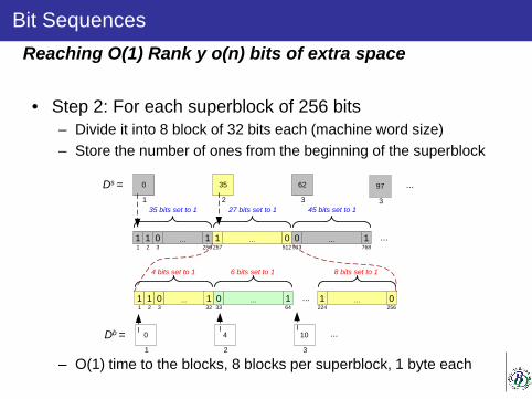
• Step 2: For each superblock of 256 bits – Divide it into 8 block of 32 bits each (machine word size) – Store the number of ones from the beginning of the superblock
– O(1) time to the blocks, 8 blocks per superblock, 1 byte each
Reaching O(1) Rank y o(n) bits of extra space
1 1 0 ... 11 2 3 256
35 bits set to 1
1 ... 0257 512 27 bits set to 1
350
1 2
Ds = 62
3
0 ... 1513 768
45 bits set to 1
...
97
3
...
1 1 0 ... 11 2 3 32
4 bits set to 1
0 ... 133 64
6 bits set to 1
...
40
1 2
Db = 10
3
...
1 ... 0224 256
8 bits set to 1

Bit Sequences
• Step 3: Rank within a 32 bit block
Finally solving: rank1( D , p ) = Ds[ p / 256 ] + Db[ p / 32 ] + rank1(blk, i) where i= p mod 32
– Ex: rank1(D,300) = 35 + 4 + 4 = 43
– Yet, how to compute rank1(blk, i) in constant time ?
Reaching O(1) Rank y o(n) bits of extra space
1 0 0 1 0 0 0 0 1 1 0 0 0 1 0 1 1 0 0 0 0 1 0 0 0 1 1 0 0 1 0 1blk =1 2 3 4 5 6 7 8 9 10 11 12 13 14 15 16 17 18 19 20 21 22 23 24 25 26 27 28 29 30 31 32

Bit Sequences
• how to compute rank1 (blk, i) in constant time ? – Option 1: popcount within a machine word
– Option 2: Universal Table onesInByte (solution for each byte)
Only 256 entries storing values [0..8]
• Finally sum value onesInByte for the 4 bytes in blk
• Overall space: 1.375 n bits
Reaching O(1) Rank y o(n) bits of extra space
1 0 0 1 0 0 0 0 1 1 0 0 0 1 0 1 1 0 0 0 0 1 0 0 0 1 1 0 0 1 0 1blk =1 2 3 4 5 6 7 8 9 10 11 12 13 14 15 16 17 18 19 20 21 22 23 24 25 26 27 28 29 30 31 32
0 0 0 0 0 0 0 00 0 0 0 0 0 0 0 0 0 0 0blks =1 2 3 4 5 6 7 8 9 10 11 12 13 14 15 16 17 18 19 20 21 22 23 24 25 26 27 28 29 30 31 32
1 0 0 1 0 0 0 0 1 1 0 0
Shift 32 – 12 = 20 posicións
Rank1(blk,12)Val binary OnesInByte
0 00000000 0
1 00000001 1
2 00000010 1
3 00000011 2
252 11111100 6
253 11111101 7
254 11111110 7
255 11111111 8
... ... ...

Bit Sequences
select1(p) • In practice, binary search using rank
– Binary search on superblocks O(log(n)) to find the superblock s containing the pth 1 retval = Ds[s]
– Sequential search [uint <=256] within the in blocks until reaching the block d that contains the position retval += Db[d]
– Sequential search (1 byte at a time) within the last 32 bits, using onesInByte[] table until reaching the byte b that contains the position.
• In each iteration: retval += onesInByte[b] – Table lookup over a new selb[] table over the last “byte” b
• retval += selb[b] – Return retval
Select in O(log (n)) with the same structures

Bit Sequences
• Compressed bitmap representations exist.
– Compressed [Raman et al]
– For very sparse bitmaps [Okanohara and Sadakane]
– …
Compressed representations

Outline
Introduction Basic compression Sequences
Bit sequences Integer sequences
A brief Review about Indexing

Integer Sequences Access/rank/select on general sequences
Rank2(9) = 3
S=
select4(3) =7
access (13) = 3
4 4 3 2 6 2 4 2 4 1 1 2 3 5 1 2 3 4 5 6 7 8 9 10 11 12 13 14

Integer Sequences
• Grossi et al. • Given a sequence of symbols and an encoding
– The bits of the code of each symbol are distributed along the different levels of the tree
00 01 00 10 11 00 A B A C D A C 0 0 0 0
10 1 1
0 1
A B A A C D C 0 1 0 1 0 0
1
0
Wavelet tree (construction)
DATA
SYMBOL CODE
WAVELET TREE A B A C D A C
C
D
00
01
10
11
B A

• Searching for the 1st occurrence of ‘D’?
Integer Sequences
DATA
SYMBOL CODE
WAVELET TREE A B A C D A C
C
D
00
01
10
11
B A
A B A C D A C 0 0 0 0 1 1
0 1
A B A A C D C 0 1 0 1 0 0
it is the 2nd bit in B1
Where is the 2nd ‘1’? at pos 5.
0
1
Where is the 1st ‘1’? at pos 2.
Wavelet tree (select)
Broot
B0 B1

Integer Sequences
• Recovering Data: extracting the next symbol – Which symbol appears in the 6th position?
A B A C D A C 0 0 0 0 1 1
0 1
A B A A C D C 0 1 0 1 0 0
Which bit occus at position 4 in B0?
How many ‘0’s are there up to pos 6? it is the 4th ‘0’
0
1
It is set to 0
The codeword read is ’00’ A
Wavelet tree (access)
DATA
SYMBOL CODE
WAVELET TREE A B A C D A C
C
D
00
01
10
11
B A
Broot
B0 B1
Broot
B0 B1
Broot
B0

Integer Sequences
• Recovering Data: extracting the next symbol – Which symbol appears in the 7th position?
A B A C D A C 0 0 0 0 1 1
0 1
A B A A C D C 0 1 0 1 0 0
Which bit occurs at position 3 in B1?
How many ‘1’s are there up to pos 7?
it is the 3rd ‘1’
0
1
It is set to 0
The codeword read is ’10’ C
TEXT
SYMBOL CODE
WAVELET TREE A B A C D A C
C
D
00
01
10
11
B A
Wavelet tree (access)
B1
Broot
B0

Integer Sequences
• How many C’s up to position 7?
A B A C D A C 0 0 0 0 1 1
0 1
A B A A C D C 0 1 0 1 0 0
How many 0s up to position 3 in B1?
How many ‘1’s are there up to pos 7?
it is the 3rd ‘1’
0
1
2 !!
TEXT
SYMBOL CODE
WAVELET TREE A B A C D A C
C
D
00
01
10
11
B A
Wavelet tree (Rank)
B1
Broot
B0
Select (locate symbol)
Access and Rank:

Integer Sequences
• Each level contains n + o(n) bits
• Rank/select/access expected O(log σ) time
A B A C D A C 0 0 0 0 1 1
0 1
A B A A C D C 0 1 0 1 0 0
1
0
Wavelet tree (Space and times)
WAVELET TREE
00 01 00 10 11 00 10 DATA
SYMBOL CODE
A B A C D A C
C
D
00
01
10
11
B A n + o(n) bits
n + o(n) bits
n ⌈log σ⌉ (1 + o(1)) bits

Integer Sequences
• Using Huffman coding (or others) umbalanced
• Rank/select/access O(nH0(S)) time
Huffman-shaped (or others) Wavelet tree
A B A C D A C 1 0 1 1 0 0
0 1
B C D C A A A 0 1 0 0
0
WAVELET TREE
1 000 1 01 001 1 01 DATA
SYMBOL CODE
A B A C D A C
C
D
1
000
01
001
B A
nH0(S) + o(n) bits
0 1
B D C C 1 0

Outline
Introduction Basic compression Sequences
Bit sequences Integer sequences
A brief Review about Indexing

A brief Review about Indexing
• Traditional indexes (with or without compression)
– Inverted Indexes, Suffix Arrays,...
• Compressed Self-indexes
– Wavelet trees, Compressed Suffix Arrays, FM-index, LZ-index, …
Text Indexing: Well-known structures from The Web
implicit text
auxiliar structure explicit text

A brief Review about Indexing Inverted indexes
Space-time trade-off
DCC communications
compression image data
information Cliff
Logde
0 142
104 165 341 506 368
219 445
DCC is held at the Cliff Lodge convention center. It is an international forum for current work on data compression and related applications. DCC addresses not only compression methods for specific types of data (text, image, video, audio, space, graphics, web content, etc.), but also the use of techniques from information theory and data compression in networking, communications, and storage applications involving large datasets (including image and information mining, retrieval, archiving, backup, communications, and HCI).
99 207 336 128 395 19 25
Vocabulary Posting Lists
Indexed text Searches
Word posting of that word Phrase intersection of postings B
lock
1
Blo
ck 2
Compression
- Indexed text (Huffman,...) - Posting lists (Rice,...)
1
1 2 2
1 2 1 2 1 2 1 1
DCC communications
compression image data
information Cliff
Lodge
Vocabulary Posting Lists
Full-positional information Block-addressing inverted index

A brief Review about Indexing
• Lists contain increasing integers • Gaps between integers are smaller in the longest lists
Inverted indexes
4 10 15 25 29 40 46 54 57 70 79 82 Posting list original
1 2 3 4 5 6 7 8 9 10 11 12
4 6 5 10 4 11 6 8 3 13 9 3 Diferenc.
4
c6 c5 c10
29
c11 c6 c8
57
c13 c9 c3
Sampling absoluto + codif long. variable
Acceso directo
Descompresión parcial
c4 c6 c5 c10 c4 c11 c6 c8 c3 c13 c9 c3 Codif long. variable Descompresión
completa

A brief Review about Indexing
• Sorting all the suffix of T lexicographically
Suffix Arrays
a b r a c a d a b r a $1 2 3 4 5 6 7 8 9 10 11 12
T =
12 11 8 1 4 6 9 2 5 7 10 3
1 2 3 4 5 6 7 8 9 10 11 12
A =
abracadabra$acadabra$
$ a$ adabra$bra$bracadabra$
cadabra$
abra$
dabra$
ra$racadabra$

A brief Review about Indexing
• Binary search for any pattern: “ab”
Suffix Arrays
a b r a c a d a b r a $1 2 3 4 5 6 7 8 9 10 11 12
T =
12 11 8 1 4 6 9 2 5 7 10 3
1 2 3 4 5 6 7 8 9 10 11 12
A =
P = a b

A brief Review about Indexing
• Binary search for any pattern: “ab”
Suffix Arrays
P = a b
a b r a c a d a b r a $1 2 3 4 5 6 7 8 9 10 11 12
T =
12 11 8 1 4 6 9 2 5 7 10 3
1 2 3 4 5 6 7 8 9 10 11 12
A =

A brief Review about Indexing
• Binary search for any pattern: “ab”
Suffix Arrays
P = a b
a b r a c a d a b r a $1 2 3 4 5 6 7 8 9 10 11 12
T =
12 11 8 1 4 6 9 2 5 7 10 3
1 2 3 4 5 6 7 8 9 10 11 12
A =
A brief Review about Indexing
• Binary search for any pattern: “ab”
Suffix Arrays
P = a b
a b r a c a d a b r a $1 2 3 4 5 6 7 8 9 10 11 12
T =
12 11 8 1 4 6 9 2 5 7 10 3
1 2 3 4 5 6 7 8 9 10 11 12
A =

A brief Review about Indexing
• Binary search for any pattern: “ab”
Suffix Arrays
P = a b
a b r a c a d a b r a $1 2 3 4 5 6 7 8 9 10 11 12
T =
12 11 8 1 4 6 9 2 5 7 10 3
1 2 3 4 5 6 7 8 9 10 11 12
A =

A brief Review about Indexing
• Binary search for any pattern: “ab”
Suffix Arrays
P = a b
a b r a c a d a b r a $1 2 3 4 5 6 7 8 9 10 11 12
T =
12 11 8 1 4 6 9 2 5 7 10 3
1 2 3 4 5 6 7 8 9 10 11 12
A =

A brief Review about Indexing
• Binary search for any pattern: “ab”
Suffix Arrays
P = a b
a b r a c a d a b r a $1 2 3 4 5 6 7 8 9 10 11 12
T =
12 11 8 1 4 6 9 2 5 7 10 3
1 2 3 4 5 6 7 8 9 10 11 12
A =
locations Noccs = (4-3)+1
Occs = A[3] .. A[4] = { 8, 1}
Fast space O(m lg n) O(4n) O(m lg n + noccs) + T

Basic Compression
• BWT(S) + other structures it is an index
BWT FM-index
• C[c] : for each char c in Σ , stores the number of occs in S of the chars that are lexicographically smaller than c.
C[$]=0 C[i]=1 C[m]=5 C[p]=6 C[s]=8
• OCC(c, k): Number of occs of char c the prefix of L: L (1, k)
For k in [1..12]
Occ[$] = 0,0,0,0,0,1,1,1,1,1,1,1
Occ[i] = 1,1,1,1,1,1,1,2,2,2,3,4
Occ[m] = 0,0,0,0,1,1,1,1,1,1,1,1
Occ[p] = 0,1,1,1,1,1,2,2,2,2,2,2
Occ[s] = 0,0,1,2,2,2,2,2,3,4,4,4
• Char L[i] occurs in F at position LF(i): LF(i) = C[L[i]] + Occ(L[i],i)

Basic Compression
• Count (S[1,u], P[1,p])
BWT FM-index
C[$]=0 C[i]=1 C[m]=5 C[p]=6 C[s]=8
Occ[$] = 0,0,0,0,0,1,1,1,1,1,1,1
Occ[i] = 1,1,1,1,1,1,1,2,2,2,3,4
Occ[m] = 0,0,0,0,1,1,1,1,1,1,1,1
Occ[p] = 0,1,1,1,1,1,2,2,2,2,2,2
Occ[s] = 0,0,1,2,2,2,2,2,3,4,4,4
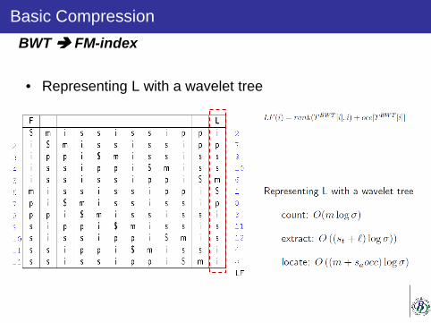
Basic Compression
• Representing L with a wavelet tree
BWT FM-index

Bibliography
1. M. Burrows and D. J. Wheeler. A block-sorting lossless data compression algorithm. Technical Report 124, Digital Systems Research Center, 1994. http://gatekeeper.dec.com/pub/DEC/SRC/researchreports/.
2. F. Claude and G. Navarro. Practical rank/select queries over arbitrary sequences. In Proc. 15th SPIRE, LNCS 5280, pages 176–187, 2008.
3. Paolo Ferragina and Giovanni Manzini. An experimental study of an opportunistic index. In Proc. 12th ACM-SIAM Symposium on Discrete Algorithms (SODA), Washington (USA), 2001.
4. Paolo Ferragina and Giovanni Manzini. Indexing compressed text. Journal of the ACM, 52(4):552-581, 2005.
5. Philip Gage. A new algorithm for data compression. C Users Journal, 12(2):23–38, February 1994
6. A. Golynski, I. Munro, and S. Rao. Rank/select operations on large alphabets: a tool for text indexing. In Proc. 17th SODA, pages 368–373, 2006.
7. R. Grossi, A. Gupta, and J. Vitter. High-order entropy-compressed text indexes. In Proc. 14th SODA, pages 841–850, 2003.

Bibliography
8. David A. Huffman. A method for the construction of minimum-redundancy codes. Proc. of the Institute of Radio Engineers, 40(9):1098-1101, 1952
9. N. J. Larsson and Alistair Moffat. Off-line dictionary-based compression. Proceedings of the IEEE, 88(11):1722–1732, 2000
10. U. Manber and G. Myers. Suffix arrays: a new method for on-line string searches. SIAM J. Comp., 22(5):935–948, 1993
11. Alistair Moffat, Andrew Turpin: Compression and Coding Algorithms .Kluwer 2002, ISBN 0-7923-7668-4
12. I. Munro. Tables. In Proc. 16th FSTTCS, LNCS 1180, pages 37–42, 1996.
13. Gonzalo Navarro , Veli Mäkinen, Compressed full-text indexes, ACM Computing Surveys (CSUR), v.39 n.1, p.2-es, 2007
14. D. Okanohara and K. Sadakane. Practical entropy-compressed rank/select dictionary. In Proc. 9th ALENEX, 2007.
15. R. Raman, V. Raman, and S. Rao. Succinct indexable dictionaries with applications to encoding k-ary trees and multisets. In Proc. 13th SODA, pages 233–242, 2002.

Bibliography
16. Edleno Silva de Moura, Gonzalo Navarro, Nivio Ziviani, and Ricardo Baeza-Yates. Fast and flexible word searching on compressed text. ACM Transactions on Information Systems, 18(2):113–139, 2000.
17. Ian H. Witten, Alistair Moffat, and Timothy C. Bell. Managing Gigabytes: Compressing and Indexing Documents and Images. Morgan Kaufmann, 1999.
18. Ziv, J. and Lempel, A. 1977. A universal algorithm for sequential data compression. IEEE Transactions on Information Theory 23, 3, 337–343.
19. Ziv, J. and Lempel, A. 1978. Compression of individual sequences via variable-rate coding. IEEE Transactions on Information Theory 24, 5, 530–536.
Onto some basics of: compression, Compact Data Structures, and
indexing
1st KEYSTONE Training School July 22th, 2015. Faculty of ICT, Malta
Antonio Fariña
Miguel A Martínez Prieto

IntroductionCompressed String Dictionaries
Experimental Evaluation
Dictionary Compression
Miguel A. Martınez-Prieto Antonio FarinaUniv. of Valladolid (Spain) Univ. of A Coruna (Spain)
[email protected] [email protected]
Keyword search over Big Data.
– 1st KEYSTONE Training School –.July 22nd, 2015. Faculty of ICT, Malta.
Miguel A. Martınez-Prieto & Antonio Farina Dictionary Compression 1/47

IntroductionCompressed String Dictionaries
Experimental Evaluation
What is a String Dictionary?OperationsRDF Dictionaries
Outline
1 Introduction
2 Compressed String Dictionaries
3 Experimental Evaluation
Miguel A. Martınez-Prieto & Antonio Farina Dictionary Compression 2/47

IntroductionCompressed String Dictionaries
Experimental Evaluation
What is a String Dictionary?OperationsRDF Dictionaries
– What is a String Dictionary –
String Dictionary
A string dictionary is a serializable data structurewhich organizes all different strings (vocabulary) usedin a dataset.
The vocabulary of a natural language text (lexicon) comprises all differentwords used in it.
T= “la tarara sı la tarara no la tarara ni~na que la he visto yo”
V= {he, la, ni~na, no, que, sı, tarara, visto, yo}
Miguel A. Martınez-Prieto & Antonio Farina Dictionary Compression 3/47
IntroductionCompressed String Dictionaries
Experimental Evaluation
What is a String Dictionary?OperationsRDF Dictionaries
What is a String Dictionary?
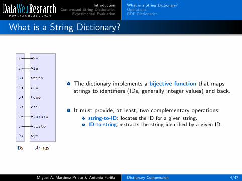
The dictionary implements a bijective function that mapsstrings to identifiers (IDs, generally integer values) and back.
It must provide, at least, two complementary operations:
string-to-ID: locates the ID for a given string.ID-to-string: extracts the string identified by a given ID.
Miguel A. Martınez-Prieto & Antonio Farina Dictionary Compression 4/47

IntroductionCompressed String Dictionaries
Experimental Evaluation
What is a String Dictionary?OperationsRDF Dictionaries
What is a String Dictionary?
String dictionaries are a simple and effective tool:
Enable replacing (long, variable-length) strings by simplenumbers (their IDs).
T= “la tarara sı la tarara no la tarara ni~na que la he visto yo”
T’= 2 7 6 2 7 4 2 7 3 5 2 1 8 9
The resulting IDs are more compact to represent and easierand more efficient to handle:
T= 59 chars × 1 byte/chars = 59 bytes
T’= 14 IDs × dlog(9)e bits/ID = 7 bytes(plus the cost of dictionary encoding)
A compact dictionary which provides efficient mappingbetween strings and IDs saves storage space, andprocessing/transmission costs, in data-intensiveapplications.
Miguel A. Martınez-Prieto & Antonio Farina Dictionary Compression 5/47

IntroductionCompressed String Dictionaries
Experimental Evaluation
What is a String Dictionary?OperationsRDF Dictionaries
Compressing String Dictionaries
The growing volume of the datasets has led to increasingly large
dictionaries:
The dictionary size is a bottleneck for applications running underrestrictions of main memory.Dictionary management is becoming a scalability issue by itself.
Dictionary compression aims to achieve competitive space/time tradeoffs:
Compact serialization.Small memory footprint.Efficient query resolution.
We focus on static dictionaries, which do not change along the
execution:Many applications use dictionaries that either are static or are rebuilt onlysparingly.
Miguel A. Martınez-Prieto & Antonio Farina Dictionary Compression 6/47
IntroductionCompressed String Dictionaries
Experimental Evaluation
What is a String Dictionary?OperationsRDF Dictionaries
– Operations –
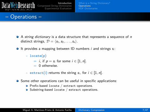
A string dictionary is a data structure that represents a sequence of ndistinct strings, D = 〈s1, s2, . . . , sn〉.
It provides a mapping between ID numbers i and strings si :
- locate(p)
= i , if p = si for some i ∈ [1, n].= 0 otherwise.
- extract(i) returns the string si , for i ∈ [1, n].
Some other operations can be useful in specific applications:
Prefix-based locate / extract operations.Substring-based locate / extract operations.
Miguel A. Martınez-Prieto & Antonio Farina Dictionary Compression 7/47

IntroductionCompressed String Dictionaries
Experimental Evaluation
What is a String Dictionary?OperationsRDF Dictionaries
Prefix-based Operations
- locatePrefix(p) = {i , ∃y , si = py}.This result set is a contiguous ID range for lexicographically sorteddictionaries.
- extractPrefix(p) = {si , ∃y , si = py}.It is equivalent to composing locatePrefix(p) with individualextract(i) operations.
Finding all URIs in a given domain is an example of prefix-based
operation:
Look for all properties used in http://dataweb.infor.uva.es/movies:http://dataweb.infor.uva.es/movies/property/director (4).http://dataweb.infor.uva.es/movies/property/name (7).http://dataweb.infor.uva.es/movies/property/title (12)....
Miguel A. Martınez-Prieto & Antonio Farina Dictionary Compression 8/47

IntroductionCompressed String Dictionaries
Experimental Evaluation
What is a String Dictionary?OperationsRDF Dictionaries
Substring-based Operations
- locateSubstring(p) = {i , ∃x , y , si = xpy}.It is very similar to the problem solved by full-text indexes.
- extractSubstring(p) = {si , ∃x , y , si = xpy}.It is equivalent to composing locateSubstring(p) with individualextract(i) operations.
Both operations may return duplicate results which must be removedbefore reporting the ID result set.
regex query resolution in SPARQL is an example of substring-based
operation:
Look for all literals containing the substring Eastwood:‘‘Clint Eastwood’’ (2544).‘‘Jayne Eastwood is a Canadian actress...’’ (10584).‘‘Kyle Eastwood’’ (13847)....
Miguel A. Martınez-Prieto & Antonio Farina Dictionary Compression 9/47

IntroductionCompressed String Dictionaries
Experimental Evaluation
What is a String Dictionary?OperationsRDF Dictionaries
Summary
- locate(“tarara”) = 7
- extract(2) = la
- locatePrefix(“n”) = 3,4
- extractPrefix(“n”) = nina, no
- locateSubstring(“a”) = 2,3,7
- extractSubstring(“a”) = la, nina, tarara
Miguel A. Martınez-Prieto & Antonio Farina Dictionary Compression 10/47

IntroductionCompressed String Dictionaries
Experimental Evaluation
What is a String Dictionary?OperationsRDF Dictionaries
– RDF Dictionaries –
An RDF dictionary comprises all different terms used in the dataset:
RDF terms are drawn from three disjoint vocabularies: URIs, Literals, andblank nodes.
Serialized (uncompressed) RDF vocabularies need up to 3 times morespace than (uncompressed) ID-triples [13].
URIs and Literals should be compressed and managed independently:
Their structure is very different and they are queried in a different way.
Miguel A. Martınez-Prieto & Antonio Farina Dictionary Compression 11/47

IntroductionCompressed String Dictionaries
Experimental Evaluation
What is a String Dictionary?OperationsRDF Dictionaries
URIs
URIs are medium-size strings sharing long prefixes:
Compressed dictionaries for URIs must exploit the continuous repetition ofsuch prefixes.Prefix-based compression.
locate operations are common when the dictionary is used for lookuppurposes (e.g. RDF stores, semantic search engines, etc.).
extract operations are common when the dictionary is used for dataaccess purposes (e.g. decompression, result retrieval, etc.).
locatePrefix and extractPrefix are also useful for URI dictionaries.
Miguel A. Martınez-Prieto & Antonio Farina Dictionary Compression 12/47

IntroductionCompressed String Dictionaries
Experimental Evaluation
What is a String Dictionary?OperationsRDF Dictionaries
Literals
Literals tends to be large-size strings with no predictable features:
The name “Clint Eastwood”.The genome from an individual of any species.The full text from “El Quijote”...
Literal dictionaries must be based on universal compression.
locate and extract are used like in URI dictionaries.
locateSubstring and extractSubstring are useful because ofSPARQL needs.
Miguel A. Martınez-Prieto & Antonio Farina Dictionary Compression 13/47

IntroductionCompressed String Dictionaries
Experimental Evaluation
What is a String Dictionary?OperationsRDF Dictionaries
Practical Configuration
A role-based partition is first performed:
Subjects are encoded in the range [1,|S|].Predicates are encoded in the range [1,|P|].Objects are encoded in the range [1,|O|].
URIs playing as subject and object are encoded
once:
IDs in [1,|SO|] encode subjects and objects.
Subjects are encoded in [|SO+1|,|S|].
Objects are encoded using two dictionaries:1 [|SO+1|,|Ox|] encode URIs which only performs
as objects.2 [|Ox+1|,|O|] encode Literals.
Miguel A. Martınez-Prieto & Antonio Farina Dictionary Compression 14/47

IntroductionCompressed String Dictionaries
Experimental Evaluation
Front-CodingHashingSelf-Indexed DictionariesOther Dictionaries
Outline
1 Introduction
2 Compressed String Dictionaries
3 Experimental Evaluation
Miguel A. Martınez-Prieto & Antonio Farina Dictionary Compression 15/47

IntroductionCompressed String Dictionaries
Experimental Evaluation
Front-CodingHashingSelf-Indexed DictionariesOther Dictionaries
Compressed String Dictionaries
All revised dictionaries combine notions from universal compression andcompact data structures.
Universal compressors must enable fast decompression and comparison of
individual strings:
Huffman [8] and Hu-Tucker [7, 9] codes.Re-Pair [10].
The serialized vocabulary Tdict concatenates all strings in lexicographic
order:
An special symbol $ is used as separator.
T =“alabar a la alabada alabarda”
Tdict = a$alabada$alabar$alabarda$la$
Miguel A. Martınez-Prieto & Antonio Farina Dictionary Compression 16/47

IntroductionCompressed String Dictionaries
Experimental Evaluation
Front-CodingHashingSelf-Indexed DictionariesOther Dictionaries
– Front-Coding –
Front-Coding [15] is a folklore compression technique for lexicographicallysorted dictionaries.
It exploits the fact that consecutive entries are likely to share a common
prefix:
Each entry in the dictionary is differentially encoded with respect to thepreceding one.It needs two values:× An integer encoding the length of the shared prefix.× The remaining characters of the current entry.
a$alabada$alabar$alabarda$la$
→ (0,a$); (1,labada$); (5, r$); (6, da$); (0, la$)
Miguel A. Martınez-Prieto & Antonio Farina Dictionary Compression 17/47

IntroductionCompressed String Dictionaries
Experimental Evaluation
Front-CodingHashingSelf-Indexed DictionariesOther Dictionaries
Front-Coding
The vocabulary is divided into buckets of b strings:
The first string of each bucket (header) is explicitly stored.The remaining b − 1 internal strings are differentially encoded.
Miguel A. Martınez-Prieto & Antonio Farina Dictionary Compression 18/47

IntroductionCompressed String Dictionaries
Experimental Evaluation
Front-CodingHashingSelf-Indexed DictionariesOther Dictionaries
Front-Coding Operations
locate(p):
1 Headers are binary searched until finding the bucket Bx where p must lie:If the header is p, locate(p) = (b × (Bx − 1)) + 1.
2 The internal string are sequentially decoded:If the internal i th string is p, locate(p) = (b × (Bx − 1)) + i .If the bucket is fully decoded with no result, p is not in the dictionary.
extract(i):1 The string is encoded in the bucket Bx = di/be.2 ((i − 1) mod b) internal strings are decoded to obtain the answer.
Prefix-based operations exploits the lexicographic order:Their results are contiguous ranges in the dictionary.
Miguel A. Martınez-Prieto & Antonio Farina Dictionary Compression 19/47

IntroductionCompressed String Dictionaries
Experimental Evaluation
Front-CodingHashingSelf-Indexed DictionariesOther Dictionaries
Plain Front-Coding (PFC)
PFC is a straightforward byte-oriented Front-Coding implementation:
It uses VByte [14] to encode the length of the common prefix.The remaining string is encoded with one byte per character, plus theterminator $.
PFC is serialized as a byte array (Tpfc) and a ptrs structure:
Both structures are directly mapped to main memory for data retrievalpurposes.
Miguel A. Martınez-Prieto & Antonio Farina Dictionary Compression 20/47

IntroductionCompressed String Dictionaries
Experimental Evaluation
Front-CodingHashingSelf-Indexed DictionariesOther Dictionaries
HuTucker Front-Coding (HTFC)
HTFC is algorithmically similar to PFC, but it takes advantage of the Tpfcredundancy to achieve a more compressed representation:
Operations are slightly slower than for PFC.
Headers are encoded using HuTucker:
It allows compressed headers to be directly compared with the querypattern.
Internal strings are encoded using Huffman or Re-Pair compression.
HTFC is serialized as a bit array (Thtfc) and also a ptrs structure:
Pointers in HTFC uses less bits because Thtfc is smaller than Tpfc .
Miguel A. Martınez-Prieto & Antonio Farina Dictionary Compression 21/47

IntroductionCompressed String Dictionaries
Experimental Evaluation
Front-CodingHashingSelf-Indexed DictionariesOther Dictionaries
– Hashing –
Hashing [3] is a folklore method to implement dictionaries:
A hash function transforms the string into an index x in the hash table.A collision arises when two different strings are mapped to the same cellin the table.
String dictionaries perform better with closed hashing [2]:
If the corresponding cell is not empty, one successively probes other cellsuntil finding a free cell.The next cell to be probed is determined using double hashing.
Hash dictionaries provide very efficient locate, may support extract,but the table size dissuades their use for managing large vocabularies.
Compressed hash dictionaries focuses on compacting the table, but
also the own vocabulary:
The vocabulary can be effectively compressed using Huffman or Re-Pair.
Miguel A. Martınez-Prieto & Antonio Farina Dictionary Compression 22/47

IntroductionCompressed String Dictionaries
Experimental Evaluation
Front-CodingHashingSelf-Indexed DictionariesOther Dictionaries
Vocabulary Compression
Miguel A. Martınez-Prieto & Antonio Farina Dictionary Compression 23/47

IntroductionCompressed String Dictionaries
Experimental Evaluation
Front-CodingHashingSelf-Indexed DictionariesOther Dictionaries
Table Compression (I)
Miguel A. Martınez-Prieto & Antonio Farina Dictionary Compression 24/47

IntroductionCompressed String Dictionaries
Experimental Evaluation
Front-CodingHashingSelf-Indexed DictionariesOther Dictionaries
Table Compression (II)
Miguel A. Martınez-Prieto & Antonio Farina Dictionary Compression 25/47

IntroductionCompressed String Dictionaries
Experimental Evaluation
Front-CodingHashingSelf-Indexed DictionariesOther Dictionaries
Improving Data Access
Miguel A. Martınez-Prieto & Antonio Farina Dictionary Compression 26/47

IntroductionCompressed String Dictionaries
Experimental Evaluation
Front-CodingHashingSelf-Indexed DictionariesOther Dictionaries
Hashing Operations (locate)
locate(p):1 The pattern p is compressed using Huffman: cp .2 cp is “hashed” to a position x in the (original) hash table.3 x is mapped to its corresponding position y in the compressed
representation.4 The string pointed from y is decompressed and compared to p.
locate(“alabada”)
1 Huffman(“alabada$”)=cp
2 hash(cp)=5
3 if B[5] = 1, rank1(B, 5)=4
if B[5] = 0, “alabada” is not in D.
4 strcmp(DAC[4],cp)=true → 4
strcmp(DAC[4],cp)=false → collision
Miguel A. Martınez-Prieto & Antonio Farina Dictionary Compression 27/47

IntroductionCompressed String Dictionaries
Experimental Evaluation
Front-CodingHashingSelf-Indexed DictionariesOther Dictionaries
Hashing Operations (extract)
extract(i):1 The string directly extract from DAC[i].
Miguel A. Martınez-Prieto & Antonio Farina Dictionary Compression 28/47

IntroductionCompressed String Dictionaries
Experimental Evaluation
Front-CodingHashingSelf-Indexed DictionariesOther Dictionaries
– Self-Indexed Dictionaries –
A self-index stores the original text T and provides indexed searches toit, using space proportional to the T statistical entropy.
Self-indexes support two operations:
locate(p), returns all the positions in T where p occurs.extract(i , j), retrieves the substring T [i , j].
A string dictionary can be easily self-indexed:
The corresponding self-index is built on the text Tdict .The dictionary primitives (and also prefix and substring based queries) areimplemented using the self-index operations.
We choose the FM-Index [4, 5] because it is the most space-efficient
self-index in practice:
A $ symbol is prepended to the original Tdict .The BWT (L) is a wavelet-tree (“plain” [5] and “compressed” [11]).C is a simple array.
Miguel A. Martınez-Prieto & Antonio Farina Dictionary Compression 29/47

IntroductionCompressed String Dictionaries
Experimental Evaluation
Front-CodingHashingSelf-Indexed DictionariesOther Dictionaries
FM-Index Dictionary
Miguel A. Martınez-Prieto & Antonio Farina Dictionary Compression 30/47

IntroductionCompressed String Dictionaries
Experimental Evaluation
Front-CodingHashingSelf-Indexed DictionariesOther Dictionaries
FM-Index Dictionary (locate)
The i th string is encoded between thei + 1th and i + 2th $.
locate(p) performs backwards search
of $p$:
The pattern is searched from right toleft until reach the corresponding $.
locate(p) performs in timeO(|p| log σ).
Miguel A. Martınez-Prieto & Antonio Farina Dictionary Compression 31/47

IntroductionCompressed String Dictionaries
Experimental Evaluation
Front-CodingHashingSelf-Indexed DictionariesOther Dictionaries
FM-Index Dictionary (locate)
locate(’la’): Looking for $la$.
1. Range: [C($),C(a)-1]=[0,5].Count the number of a before the range:occs0=ranka(L, 0) = 0Count the number of a to the end of the range:occs1=ranka(L, 5) = 4
2. Range: [C(a)+occs0,C(a)+occs1-1]=[6,9].Count the number of l before the range:occs0=rankl (L, 6) = 0Count the number of a to the end of the range:occs1=rankl (L, 9) = 1
3. Range: [C(l)+occs0,C(l)+occs1-1]=[24,25].Count the number of l before the range:occs0=rank$(L, 24) = 5Count the number of a to the end of the range:occs1=rank$(L, 25) = 6
4. Range: [C($)+occs0,C($)+occs1-1]=[5,5].
’la’ is identified by 5.
Miguel A. Martınez-Prieto & Antonio Farina Dictionary Compression 32/47

IntroductionCompressed String Dictionaries
Experimental Evaluation
Front-CodingHashingSelf-Indexed DictionariesOther Dictionaries
FM-Index Dictionary (extract)
extract(i) retrieves symbols from the
(i + 1)− th $ to the i − th $:
It takes O(|si | log σ) time.
extract(5):
1. The search process starts from Position: 0.Extracts the symbol in this position:access(L, 0) =aCount the number of as up to the position:occs=ranka(L, 0) = 1
2. Position: C(a) + 1− 1 = 6.Extracts the symbol in this position:access(L, 6) =lCount the number of ls up to the position:occs=rankl (L, 6) = 1
3. Position: C(l) + 1− 1 = 24.Extracts the symbol in this position:
access(L, 6) =$
The 5− th string is la.
Miguel A. Martınez-Prieto & Antonio Farina Dictionary Compression 33/47

IntroductionCompressed String Dictionaries
Experimental Evaluation
Front-CodingHashingSelf-Indexed DictionariesOther Dictionaries
FM-Index Dictionary (prefix & substring operations)
locatePrefix(p) is similar to locate:
It looks for $p and finds the area[sp,ep] in where all strings si thatstart with p are encoded.
Substring-based operations generalize
prefix-based ones:
locateSubstring(p) look for p toobtain the area [sp,ep] containing allstrings si with p.For each match, the backwards searchcontinues until determining thecorresponding ID (sampling structure)Duplicate IDs are finally removed.
extractPrefix(p) andextractSubstring(p) perform extract
operations in the corresponding ranges.
Miguel A. Martınez-Prieto & Antonio Farina Dictionary Compression 34/47

IntroductionCompressed String Dictionaries
Experimental Evaluation
Front-CodingHashingSelf-Indexed DictionariesOther Dictionaries
– Other Dictionaries (Tries)–
Tries [9] are tree-shaped structures which perform
efficiently for dictionary purposes:
Strings are located from root to leaves.IDs are extracted from the corresponding leaf to theroot.
Tries use much space for managing large dictionaries.
Some compressed trie-based dictionaries exist in the
state of the art:
Compressed tries based on path decomposition [6].LZ-compressed tries [1].Self-indexed tries (XBW) [2].
Miguel A. Martınez-Prieto & Antonio Farina Dictionary Compression 35/47

IntroductionCompressed String Dictionaries
Experimental Evaluation
URIsLiteralsConclusions
Outline
1 Introduction
2 Compressed String Dictionaries
3 Experimental Evaluation
Miguel A. Martınez-Prieto & Antonio Farina Dictionary Compression 36/47

IntroductionCompressed String Dictionaries
Experimental Evaluation
URIsLiteralsConclusions
Experimental Setup
Two RDF real-world dictionaries:
26, 948, 638 URIs from Uniprot:
Averaged length: 51.04 chars per URI.Highly-repetitive.
27, 592, 013 Literals from DBpedia:
Averaged length: 60.45 chars per Literal.
We analyze compression effectiveness and retrieval speed:
locate, extract.Prefix-based operations (URIs)Substring-based operations (Literals).
In practice, extract is the most important query:
It is used many times as results are retrieved from the compressed dataset.
Miguel A. Martınez-Prieto & Antonio Farina Dictionary Compression 37/47
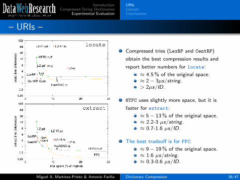
IntroductionCompressed String Dictionaries
Experimental Evaluation
URIsLiteralsConclusions
– URIs –
Compressed tries (LexRP and CentRP)
obtain the best compression results and
report better numbers for locate:
≈ 4.5 % of the original space.≈ 2− 3µs/string .> 2µs/ID.
HTFC uses slightly more space, but it is
faster for extract:
≈ 5− 13 % of the original space.≈ 2.2-3 µs/string .≈ 0.7-1.6 µs/ID.
The best tradeoff is for PFC:
≈ 9− 19 % of the original space.≈ 1.6 µs/string .≈ 0.3-0.6 µs/ID.
Miguel A. Martınez-Prieto & Antonio Farina Dictionary Compression 38/47

IntroductionCompressed String Dictionaries
Experimental Evaluation
URIsLiteralsConclusions
Prefix-based Operations
PFC is the best choice for prefix-based operations:
Although it uses more space, it reports the best performance.
Miguel A. Martınez-Prieto & Antonio Farina Dictionary Compression 39/47

IntroductionCompressed String Dictionaries
Experimental Evaluation
URIsLiteralsConclusions
– Literals –
Compressed tries (LexRP and CentRP)
obtain better compression results and
report better numbers for locate:
≈ 12 % of the original space.≈ 2-2.5 µs/string .> 2.5 µs/ID.
HTFC reports the best compression ratios,
but its performance is less competitive:
≈ 9− 17 % of the original space.≈ 4.5-40 µs/string .≈ 3− 20µs/ID.
The best tradeoff is for Hash:
≈ 15 % of the original space.≈ 1.5 µs/string .≈ 1µs/ID.
Miguel A. Martınez-Prieto & Antonio Farina Dictionary Compression 40/47

IntroductionCompressed String Dictionaries
Experimental Evaluation
URIsLiteralsConclusions
Substring-based Operations
Miguel A. Martınez-Prieto & Antonio Farina Dictionary Compression 41/47

IntroductionCompressed String Dictionaries
Experimental Evaluation
URIsLiteralsConclusions
– Conclusions –
RDF dictionaries are highly compressible:
URIs are very redundant and Literals also show non-negligible symbolicredundancy.
This redundancy can be detected and removed within specific data
structures for dictionaries:
Structures for URIs use up to 20 times less space than the originaldictionaries.For Literals, the corresponding structures use 6− 8 times less space thanthe original dictionaries.
All these structures report data retrieval performance at microsecond
level:
This functionality includes both simple and advanced operations.
Miguel A. Martınez-Prieto & Antonio Farina Dictionary Compression 42/47

IntroductionCompressed String Dictionaries
Experimental Evaluation
URIsLiteralsConclusions
GitHub
All dictionaries explained in this lecture (and some more [12]) areavailable in the libCSD C++ library:
https://github.com/migumar2/libCSD
Beta version: suggestions are accepted ;)
Miguel A. Martınez-Prieto & Antonio Farina Dictionary Compression 43/47

IntroductionCompressed String Dictionaries
Experimental Evaluation
URIsLiteralsConclusions
Bibliography I
[1] Julian Arz and Johannes Fischer.LZ-compressed string dictionaries.In Procedings of DCC, pages 322–331, 2014.
[2] Nieves Brisaboa, Rodrigo Canovas, Francisco Claude, Miguel A. Martınez-Prieto, and Gonzalo Navarro.Compressed string dictionaries.In Proceedings of SEA, pages 136–147, 2011.
[3] Thomas H. Cormen, Charles E. Leiserson, Ronald L. Rivest, and Clifford Stein.Introduction to Algorithms.MIT Press and McGraw-Hill, 2nd edition, 2001.
[4] Paolo Ferragina and Giovanni Manzini.Indexing compressed texts.Journal of the ACM, 52(4):552–581, 2005.
[5] Paolo Ferragina, Giovanni Manzini, Veli Makinen, and Gonzalo Navarro.Compressed representations of sequences and full-text indexes.ACM Transactions on Algorithms, 3(2):article 20, 2007.
[6] Roberto Grossi and Giuseppe Ottaviano.Fast Compressed Tries through Path Decompositions.In Proceedings of ALENEX, pages 65–74, 2012.
[7] T.C. Hu and Alan C. Tucker.Optimal Computer-Search Trees and Variable-Length Alphabetic Codes.SIAM Journal of Applied Mathematics, 21:514–532, 1971.
Miguel A. Martınez-Prieto & Antonio Farina Dictionary Compression 44/47

IntroductionCompressed String Dictionaries
Experimental Evaluation
URIsLiteralsConclusions
Bibliography II
[8] David A. Huffman.A method for the construction of minimum-redundancy codes.Proc. of the Institute of Radio Engineers, 40(9):1098–1101, 1952.
[9] Donald .E. Knuth.The Art of Computer Programming, volume 3: Sorting and Searching.Addison Wesley, 1973.
[10] N. Jesper Larsson and Alistair Moffat.Offline dictionary-based compression.Proceedings of the IEEE, 88:1722–1732, 2000.
[11] Veli Makinen and Gonzalo Navarro.Dynamic entropy-compressed sequences and full-text indexes.ACM Transactions on Algorithms, 4(3):article 32, 2008.
[12] Miguel A. Martınez-Prieto, Nieves Brisaboa, Rodrigo Canovas, Francisco Claude, and Gonzalo Navarro.Practical compressed string dictionaries.Information Systems, 2015.Under review.
[13] Miguel A. Martınez-Prieto, Javier D. Fernandez, and Rodrigo Canovas.Querying RDF Dictionaries in Compressed Space.SIGAPP Applied Computing Review, 12(2):64–77, 2012.
[14] Hugh E. Williams and Justin Zobel.Compressing integers for fast file access.The Computer Journal, 42:193–201, 1999.
Miguel A. Martınez-Prieto & Antonio Farina Dictionary Compression 45/47

IntroductionCompressed String Dictionaries
Experimental Evaluation
URIsLiteralsConclusions
Bibliography III
[15] Ian H. Witten, Alistair Moffat, and Timothy C. Bell.Managing Gigabytes: Compressing and Indexing Documents and Images.Morgan Kaufmann, 1999.
Miguel A. Martınez-Prieto & Antonio Farina Dictionary Compression 46/47

IntroductionCompressed String Dictionaries
Experimental Evaluation
URIsLiteralsConclusions
This presentation has been made only for learning/teaching purposes.The pictures used in the slides may be owned by other parties, so their property is exclusively of their authors.
Miguel A. Martınez-Prieto & Antonio Farina Dictionary Compression 47/47

Triples Compression and Indexing
1st KEYSTONE Training School July 22th, 2015. Faculty of ICT, Malta
Antonio Fariña
Miguel A Martínez Prieto

Outline
RDF management overview K2-Tree structure K2-Triples Compressed Suffix Array (CSA-Sad) RDF-CSA Experiments

RDF management Overview Dictionary + triples-IDS
UK
London
M.Lalmas R.Raman A.Gionis
inv-speaker Finland
SPIREheld on
capi
tal o
f
lives in
lives inposition liv
es in
attends
attends
attendsworks in
(SPIRE, held on, London)(London, capital of, UK)(A.Gionis, attends, SPIRE)(R.Raman, attends, SPIRE)(M.Lalmas, attends, SPIRE)(M.Lalmas, lives in, UK)(M.Lalmas, works in, London)(A.Gionis, lives in, Finland)(R.Raman, lives in, UK)(R.Raman, position, inv-speaker)
Original Triplets
LondonSPIREA.GionisM.LalmasR.RamanFinlandinv-speakerUK
attendscapital of
12345345
12
held onlives inpositionworks in
3456
SO
S
O
P
Dictionary Encoding
(2,3,1)(1,2,5)(3,1,2)(5,1,2)(4,1,2)(4,4,5)(4,6,1)(3,4,3)(5,4,5)(5,5,4)
Id-based Triplets

Outline
RDF management overview K2-Tree Data Structure K2-Triples Compressed Suffix Array (CSA-Sad) RDF-CSA Experiments

K2-Tree
• Structure for representing adjacency matrix • Originally designed for web graphs
– Simple directed graph
1
2
3
7
4
5
6
8
0 1 0 0 0 0 0 0 0 0 0
0 0 1 1 1 0 0 0 0 0 0
0 0 0 0 0 0 0 0 0 0 0
0 0 0 0 0 0 0 0 0 0 0
0 0 0 0 0 0 0 0 0 0 0
0 0 0 0 0 0 0 0 0 0 0
0 0 0 0 0 0 0 0 0 0 0
0 0 0 0 0 0 1 0 0 0 0
0 0 0 0 0 0 1 0 0 1 0
0 0 0 0 0 0 1 0 1 0 1
0 0 0 0 0 0 1 0 0 1 0
1 2 3 4 5 6 7 8 9 10 11
1
2
3
4
5
6
7
8
9
10
11 9
10
11
0 1 0 0 0 0 0 0 0 0 0
0 0 1 1 1 0 0 0 0 0 0
0 0 0 0 0 0 0 0 0 0 0
0 0 0 0 0 0 0 0 0 0 0
0 0 0 0 0 0 0 0 0 0 0
0 0 0 0 0 0 0 0 0 0 0
0 0 0 0 0 0 0 0 0 0 0
0 0 0 0 0 0 1 0 0 0 0
0 0 0 0 0 0 1 0 0 1 0
0 0 0 0 0 0 1 0 1 0 1
0 0 0 0 0 0 1 0 0 1 0
Motivation
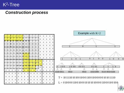
0 1 0 0 0 0 0 0 0 0 0 0 0 0 0 0
0 0 1 1 1 0 0 0 0 0 0 0 0 0 0 0
0 0 0 0 0 0 0 0 0 0 0 0 0 0 0 0
0 0 0 0 0 0 0 0 0 0 0 0 0 0 0 0
0 0 0 0 0 0 0 0 0 0 0 0 0 0 0 0
0 0 0 0 0 0 0 0 0 0 0 0 0 0 0 0
0 0 0 0 0 0 0 0 0 0 0 0 0 0 0 0
0 0 0 0 0 0 1 0 0 0 0 0 0 0 0 0
0 0 0 0 0 0 1 0 0 1 0 0 0 0 0 0
0 0 0 0 0 0 1 0 1 0 1 0 0 0 0 0
0 0 0 0 0 0 1 0 0 1 0 0 0 0 0 0
0 0 0 0 0 0 0 0 0 0 0 0 0 0 0 0
0 0 0 0 0 0 0 0 0 0 0 0 0 0 0 0
0 0 0 0 0 0 0 0 0 0 0 0 0 0 0 0
0 0 0 0 0 0 0 0 0 0 0 0 0 0 0 0
0 0 0 0 0 0 0 0 0 0 0 0 0 0 0 0
01 1 1
1 1 10 0 0 01 0 0 01
1 1 1111 1 1 10 0 0 00 0 0 0 0 0 0
0100 01000011 0010 0010 10101000 0110 0010
Example with K=2
T = 101111010100100011001000000101011110
L = 010000110010001010101000011000100100
K2-Tree Construction process

K2-Tree
0 1 0 0 0 0 0 0 0 0 0 0 0 0 0 0
0 0 1 1 1 0 0 0 0 0 0 0 0 0 0 0
0 0 0 0 0 0 0 0 0 0 0 0 0 0 0 0
0 0 0 0 0 0 0 0 0 0 0 0 0 0 0 0
0 0 0 0 0 0 0 0 0 0 0 0 0 0 0 0
0 0 0 0 0 0 0 0 0 0 0 0 0 0 0 0
0 0 0 0 0 0 0 0 0 0 0 0 0 0 0 0
0 0 0 0 0 0 1 0 0 0 0 0 0 0 0 0
0 0 0 0 0 0 1 0 0 1 0 0 0 0 0 0
0 0 0 0 0 0 1 0 1 0 1 0 0 0 0 0
0 0 0 0 0 0 1 0 0 1 0 0 0 0 0 0
0 0 0 0 0 0 0 0 0 0 0 0 0 0 0 0
0 0 0 0 0 0 0 0 0 0 0 0 0 0 0 0
0 0 0 0 0 0 0 0 0 0 0 0 0 0 0 0
0 0 0 0 0 0 0 0 0 0 0 0 0 0 0 0
0 0 0 0 0 0 0 0 0 0 0 0 0 0 0 0
01 1 1
1 1 10 0 0 01 0 0 01
1 1 1111 1 1 10 0 0 00 0 0 0 0 0 0
0100 01000011 0010 0010 10101000 0110 0010
T = 101111010100100011001000000101011110
L = 010000110010001010101000011000100100
0 1 2 3 4 5 6 7 8 9 10 11 12 13 14 15
0
1
2
3
4
5
6
7
8
9
10
11
12
13
14
15 children(2) = rank1(T,2)* k2 = 2*4=8
0 2 4 6 8 10 12 14 16 18 20 22 24 26 28 30…
children(9) = rank1(T,9)* k2 = 7*4=28
Direct neighbour operation

Outline
RDF management overview K2-Tree structure K2-Triples Compressed Suffix Array (CSA-Sad) RDF-CSA Experiments

K2-Triples
RDF triples Mapped triples Dictionary
• Dictionary encoding • Triples as a set of identifiers
Data Structure
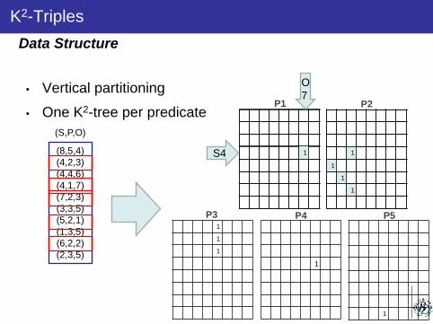
K2-Triples
• Vertical partitioning
• One K2-tree per predicate
1 (8,5,4)
(4,2,3) (4,4,6) (4,1,7) (7,2,3) (3,3,5) (5,2,1) (1,3,5) (6,2,2) (2,3,5)
1
1
1
1
1
1
1
1
1
P1 P2
P3 P4 P5
(S,P,O)
1 1
1
1
1
S4
O 7
Data Structure

K2-Triples
Query: (4,2,3)
1
1
1
1
P2
1
1
1
1
Result: (4,2,3)
• SPO checking a cell
• SP?
• ?PO
• S?O
• S??
• ??O
• ?P?
Operations

K2-Triples
Query: (4,2,?)
1
1
1
1
P2
1
1
1
1
Result: (4,2,3)
• SPO checking a cell
• SP? direct neighbours
• ?PO
• S?O
• S??
• ??O
• ?P?
Operations

K2-Triples
Query: (?,2,3)
1
1
1
1
P2
1
1
1
1
Result: (4,2,3), (7,2,3)
• SPO checking a cell
• SP? direct neighbours
• ?PO reverse neighbours
• S?O
• S??
• ??O
• ?P?
Operations

K2-Triples
Query: (4,?,6)
Result: (4,4,6)
1 1
1
1
1
1
1
1
1
1
P3 P4 P5
1 1
1
1
1
P1 P2
• SPO checking a cell
• SP? direct neighbours
• ?PO reverse neighbours
• S?O checking |P| cells
• S??
• ??O
• ?P?
Operations

K2-Triples
Query: (4,?,?)
Result: (4,1,7), (4,2,3), (4,4,6)
1 1
1
1
1
1
1
1
1
1
P3 P4 P5
1 1
1
1
1
P1 P2
• SPO checking a cell
• SP? direct neighbours
• ?PO reverse neighbours • S?O checking |P| cells
• S?? |P| direct neighbours
• ??O
• ?P?
Operations

K2-Triples
Query: (?,?,4)
Result: (8,5,4)
1 1
1
1
1
1
1
1
1
1
P3 P4 P5
1 1
1
1
1
P1 P2
• SPO checking a cell
• SP? direct neighbours
• ?PO reverse neighbours • S?O checking |P| cells
• S?? |P| direct neighbours
• ??O |P| reverse neighbours
• ?P?
Operations
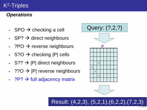
K2-Triples
Query: (?,2,?)
1
1
1
1
P2
1
1
1
1
Result: (4,2,3), (5,2,1),(6,2,2),(7,2,3)
• SPO checking a cell
• SP? direct neighbours
• ?PO reverse neighbours
• S?O checking |P| cells
• S?? |P| direct neighbours
• ??O |P| reverse neighbours
• ?P? full adjacency matrix
Operations

• Weakness of vertical partitioning unbounded predicates – (S,?,?), (?,?,O), (S,?,O)
– Checking the |P| K2-trees!
• They proposed indexes SP and OP
K2-Triples
(8,5,4) (4,2,3) (4,4,6) (4,1,7) (7,2,3) (3,3,5) (5,2,1) (1,3,5) (6,2,2) (2,3,5)
(S,P,O) S Predicates 1 3 2 3 3 3 4 1,2,4 5 2 6 2 7 2 8 5
SP INDEX
Statistically compressed Direct access with DAC
Indexes SP & OP

K2-Triples
1 1
1
1
1
1
1
1
1
1
P1 P2 P3 P4 P5
SP INDEX
Subject 4?
Predicate list: 1,2,4
• Query (4,?,?)
Indexes SP & OP

K2-Triples
Joins

• Independent join • Chain join • Interactive join
K2-Triples
• They implemented three join strategies – Taking advantage of the K2-triples structure
1
P5 (8,5,?X) (?X,2,?)
Query: (8,5,?X) (?X,2,?)
1
1
1
1
P2
Best strategy depends on the dataset and the type of join
Joins

K2-Triples
1
P5 (8,5,?X) (?X,2,?)
Query: (8,5,?X) (?X,2,?)
1
1
1
1
P2
1 0 1
1
1
1
1 0
X[1-4]
X[5-8]
X[1-4]
X[5-8]
P5 P2
Joins > Interactive Join

• Real datasets from different domains
• Space results (Mbytes)
K2-Triples
Dataset Size(MB) #Triples #Predicates #Subjects #Objects Jamendo 144.18 1,049,639 28 335,926 440,604 DBLP 7.58 46,597,620 27 2,840,639 19,639,731 Geonames 12,347.70 112,235,492 26 8,147,136 41,111,569 Dbpedia 33,912.71 232,542,405 39,672 18,425,128 65,200,769
Dataset MonetDB RDF-3X Hexastore K2-triples K2-triples+ Jamendo 8.76 37.73 1,371.25 0.74 1.28 DBLP 358.44 1,643.31 82.48 99.24 Geonames 859.66 3,584.80 152.20 188.63 Dbpedia 1,811.74 9,757.58 931.44 1178.38
Experiments

K2-Triples Experiments > triple patterns
• Triple patterns (DBPEDIA)

K2-Triples
Experiments > Join

Outline
RDF management overview K2-Tree Data Structure K2-Triples Compressed Suffix Array (CSA-Sad) RDF-CSA Experiments

Compressed Suffix Array (CSA-SAD)
• Binary search for any pattern: “ab”
Back to Suffix Arrays
P = a b
a b r a c a d a b r a $1 2 3 4 5 6 7 8 9 10 11 12
T =
12 11 8 1 4 6 9 2 5 7 10 3
1 2 3 4 5 6 7 8 9 10 11 12
A =
locations Noccs = (4-3)+1
Occs = A[3] .. A[4] = { 8, 1}
Fast space O(m lg n) O(4n) O(m lg n + noccs) + T

Compressed Suffix Array (CSA-SAD)
a b r a c a d a b r a $1 2 3 4 5 6 7 8 9 10 11 12
T =
12 11 8 1 4 6 9 2 5 7 10 3
1 2 3 4 5 6 7 8 9 10 11 12
A =
abracadabra$acadabra$
$ a$ adabra$bra$bracadabra$cadabra$
abra$
dabra$ra$racadabra$
P = a b
CSA basics
• Can we reduce the space needs of a Suffix Array?

Compressed Suffix Array (CSA-SAD) CSA basics
• Ψ
• A[Ψ(i)] = A[i] +1
racadabra$a b r a c a d a b r a $1 2 3 4 5 6 7 8 9 10 11 12
T =
12 11 8 1 4 6 9 2 5 7 10 3
1 2 3 4 5 6 7 8 9 10 11 12
A =
abracadabra$acadabra$
$ a$ adabra $bra$bracadabra$cadabra$
abra$
dabra$ra$
1 2 3 4 5 6 7 8 9 10 11 12
Ψ=

Compressed Suffix Array (CSA-SAD) CSA basics
• Ψ
• A[Ψ(i)] = A[i] +1
racadabra$a b r a c a d a b r a $1 2 3 4 5 6 7 8 9 10 11 12
T =
12 11 8 1 4 6 9 2 5 7 10 3
1 2 3 4 5 6 7 8 9 10 11 12
A =
abracadabra$acadabra$
$ a$ adabra $bra$bracadabra$cadabra$
abra$
dabra$ra$
1 2 3 4 5 6 7 8 9 10 11 12
Ψ=

a b r a c a d a b r a $1 2 3 4 5 6 7 8 9 10 11 12
T =
12 11 8 1 4 6 9 2 5 7 10 3
1 2 3 4 5 6 7 8 9 10 11 12
A =
abracadabra$a cadabra$
$ a$ adabra $b ra$b racadabra $c adabra$
abra$
dabra $r a$r acadabra $
3
1 2 3 4 5 6 7 8 9 10 11 12
Ψ=
• Ψ
• A[Ψ(10)] = A[3] = A[10] +1 = 8
Compressed Suffix Array (CSA-SAD)
7
CSA basics

• Ψ and F
• Ψ and F are enought to perform binary search and to recover the source data!!
Compressed Suffix Array (CSA-SAD)
a b r a c a d a b r a $1 2 3 4 5 6 7 8 9 10 11 12
T =
12 11 8 1 4 6 9 2 5 10 3
1 2 3 4 5 6 7 8 9 10 11 12
A =
abracadabra$acadabra$
$ a$ adabra$bra$bracadabra$cadabra$
abra$
dabra$ra$racadabra$
4 1 7 8 9 10 11 12 6 2 5
1 2 3 4 5 6 7 8 9 10 11 12
Ψ= 3
7
F =
CSA basics

Compressed Suffix Array (CSA-SAD)
• Ψ and F (reducing space needs)
$ a a a a a b b c d r r
1 2 3 4 5 6 7 8 9 10 11 12
F =
1 1 0 0 0 0 1 0 1 1 1 0=D
$ a b c d r
1 2 3 4 5 6
=S
Bitmap
Sorted alphabet
CSA basics

Compressed Suffix Array (CSA-SAD)
• Ψ and F (reducing space needs)
• Example: F[8] = S[rank1(D, 8)] = S[3] = ‘b’ Rank1(D,i):: Time O(1), by using o(n) extra space
Representing F
$ a a a a a b b c d r r
1 2 3 4 5 6 7 8 9 10 11 12
F =
1 1 0 0 0 0 1 0 1 1 1 0=D
$ a b c d r
1 2 3 4 5 6
=S
Bitmap
Sorted alphabet
rank1(D, 8)

Compressed Suffix Array (CSA-SAD) Compressing Ψ
• Absolute samples (k=sample period) • Gap encoding on increasing values: Huffman & run-encoding
• Huffman with a N entries dictionary – k reserved Huffman codes to encode 1-runs of size s ϵ [1..k-1] – 32 + 32 Huffman codes representing the size (en bits) of large values [ + or - ]
• They are followd by that number encoded with log (v) bits – The remaining N – k -32 -32 entries correspond to the most frequent gap values.
11 6 7 12 1 4 9 10 8 2 3 5
1 2 3 4 5 6 7 8 9 10 11 12
Ψ =
1 0 0 1 0 0 0 00 0 1 0 0 0 1 0 1 0 0 0 0 1 11 0 1 1 0 1 0 0 1 0 1 0 10 0 1 0 0 1 0 0
11
1
1
18
8
32sΨ =
Δ =

Compressed Suffix Array (CSA-SAD)
sampling
sampling
sampling + gap encoding + - delta codes* - Huffman-based - encoding de runs
– Ψ(sampled), D, S count – A(sampled) locate – A-1(sampled) extract
1 1 0 0 0 0 1 0 1 1 1 0=D
12 11 8 1 4 6 9 2 5 10 3A = 7
4 8 12 5 9 6 10 3 7 2 1A = 11-1
4 1 7 8 9 10 11 12 6 2 5Ψ= 3
$ a b c d r=S
1 2 3 4 5 6 7 8 9 10 11 12
a b r a c a d a b r a $1 2 3 4 5 6 7 8 9 10 11 12
T =
Parameters: space/time “trade-off”
Complete structure

Outline
RDF management overview K2-Tree Data Structure K2-Triples Compressed Suffix Array (CSA-Sad) RDF-CSA Experiments
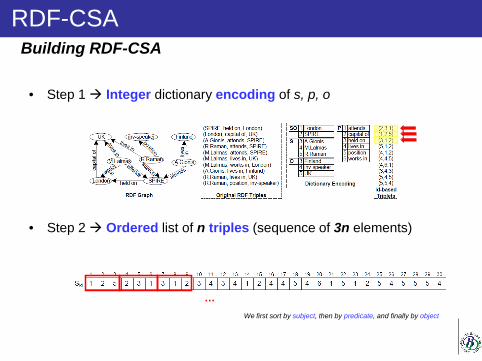
RDF-CSA
• Step 1 Integer dictionary encoding of s, p, o
• Step 2 Ordered list of n triples (sequence of 3n elements)
Building RDF-CSA
We first sort by subject, then by predicate, and finally by object
…

RDF-CSA
• Step 3 Sid is transformed into S, in order to keep disjoint alphabets
Building RDF-CSA
Range [1, ns] for subjects Range [ns+1, ns + np] for predicates Range [ns + np + 1, ns + np + no] for objects
Due to this alphabet mapping, every subject is smaller than every predicate, and this in turn is smaller than every object !!!
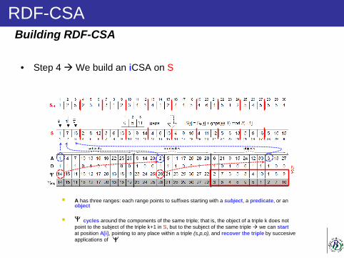
RDF-CSA
• Step 4 We build an iCSA on S
Building RDF-CSA
A has three ranges: each range points to suffixes starting with a subject, a predicate, or an object
cycles around the components of the same triple; that is, the object of a triple k does not point to the subject of the triple k+1 in S, but to the subject of the same triple we can start at position A[i], pointing to any place within a triple (s,p,o), and recover the triple by succesive applications of

RDF-CSA
• (S,P,O), (?S,P,O), (S,?P,O), (S,P,?O), (?S,?P,O), (S,?P,?O), (?S,P,?O), (?S,?P,?O)
– Patterns with just one bounded element are directly solved using select on D – Pattern (?S,?P,?O) retrieves all the triples, so it can be solved by retrieving every ith
triple, using – For the rest of the patterns: binary iCSA search
• SPO bsearch(SPO,3) • ?SOP bsearch (OP,2) … S?PO bsearch (OS,2)
– Optimizations:
• D-select+forward-check strategy: find valid intervals into S, P and O ranges, and check matches with into those intervals, starting from the shortest one.
• D-select+backward-check strategy: use binary search to limit valid intervals, instead of sequentially verifying each position of the shortest interval.
Searching for triple patterns
Optimizations are applicable to pattern (S,P,O), and those with just one unbounded term!!

RDF-CSA
• (S,P,O) optimizations
– D-select+forward-check strategy: find valid intervals into S, P and O ranges, and check matches with into those intervals, starting from the shortest one.
– D-select+backward-check strategy: use binary search to limit valid intervals, instead of sequentially verifying each position of the shortest interval.
Searching for triple patterns
180 231 301 550 600 602
10 11 12 180 200 230 231 232 300 301
550 600 601 602
S=8 P=4 O=261
SP SPO
180 231 301 550 600 602
10 11 12 180 200 230 231 232 300 301
550 600 601 602
S=8 P=4 O=261
SPO PO

RDF-CSA Experiments (dbpedia) space % VS micros/occ

RDF-CSA Experiments (dbpedia) space % VS micros/occ

RDF-CSA
• RDFCSA / K2-Triples / MonetDb / RDF3X
– SPACE • K2Triples: around 30-40% size of the uncompressed triplets • RDFCSA: around 60%.
– Similar to MonetDB, 6 times less space than RDF3X
– QUERYING SPARQL triple patterns • K2Triples: Very fast at SPO. • RDFCSA: Up to 3 orders of magnitud faster than MonetDB and RDF3X
– Faster than K2Triples (in the most used SPARQL queries, it is up to 2 orders of magnitude faster)
– Strong and predictible response times (~1-2 µsec / recovered-triplet)
Summary

Bibliography
1. Antonio Fariña, Nieves R. Brisaboa, Gonzalo Navarro, Francisco Claude, Ángeles S. Places, Eduardo Rodríguez: Word-based self-indexes for natural language text. ACM Trans. Inf. Syst. (TOIS) 30(1):1 (2012)
2. Cathrin Weiss, Panagiotis Karras, Abraham Bernstein: Hexastore: sextuple indexing for semantic web data management. PVLDB 1(1): 1008-1019 (2008)
3. Kunihiko Sadakane: New text indexing functionalities of the compressed suffix arrays. J. Algorithms 48(2): 294-313 (2003)
4. MonetDB (2013), http://www.monetdb.org
5. Nieves R. Brisaboa, Susana Ladra, Gonzalo Navarro: Compact representation of Web graphs with extended functionality. Inf. Syst. 39: 152-174 (2014)
6. Sandra Álvarez-García, Nieves R. Brisaboa, Javier D. Fernández, Miguel A. Martínez-Prieto, Gonzalo Navarro: Compressed vertical partitioning for efficient RDF management. Knowl. Inf. Syst. 44(2): 439-474 (2015)
7. Thomas Neumann, Gerhard Weikum: RDF-Stores und RDF-Query-Engines. Datenbank-Spektrum 11(1): 63-66 (2011)

Triples Compression and Indexing
1st KEYSTONE Training School July 22th, 2015. Faculty of ICT, Malta
Antonio Fariña
Miguel A Martínez Prieto