JAMCJ Appl Math ComputDOI 10.1007/s12190-013-0711-z

O R I G I NA L R E S E A R C H

Key pre-distribution in a non-uniform rectangular gridfor wireless sensor networks

Sarbari Mitra · Sourav Mukhopadhyay ·Ratna Dutta

Received: 18 May 2013© Korean Society for Computational and Applied Mathematics 2013

Abstract A deterministic key pre-distribution scheme is proposed in the paper. Thedistribution of keys to the nodes precedes a virtual arrangement of the nodes intoa non-uniform rectangular grid structure. Distribution of keys is based on projectiveplanes and pairwise connectivity. With small memory requirements, the nodes inducea network which offers a trade-off between connectivity and resilience. The impactof resilience and connectivity can be controlled by choosing the number of rows andcolumns suitably. Another significant aspect of the proposed scheme is that the pathbetween any two nodes is not unique, which leads to a well-connected network.

Keywords Key pre-distribution · Projective planes · Pairwise connectivity ·Resilience

Mathematics Subject Classification 94A60

1 Introduction

The increasing interests in the wide application of Wireless Sensor Network (WSN)has been witnessed in the past few years. WSNs are capable of collecting environ-mental readings such as temperature, light, sound, humidity and can operate unat-tended in harsh environments where human surveillance is inapplicable and risky.A large number of low-cost, small, battery-powered, resource-constraint devices,

S. Mitra (B) · S. Mukhopadhyay · R. DuttaDepartment of Mathematics, IIT, Kharagpur 721302, Indiae-mail: sarbari@maths.iitkgp.ernet.in

S. Mukhopadhyaye-mail: ratna@maths.iitkgp.ernet.in

R. Duttae-mail: sourav@maths.iitkgp.ernet.in

S. Mitra et al.

known as sensor nodes, collectively build up a sensor network in sensitive regionto gather and transmit information from the environment. The process of loadingkeys to the nodes (through which they communicate securely among themselves)prior to their deployment is termed as key pre-distribution. Key pre-distribution inWireless Sensor Network (WSN) has been an active area of research for the lastdecade. A key pre-distribution scheme (KPS) can be of three types: (i) Probabilis-tic—where the keys are chosen randomly from the key pool and are given to thenodes so that any two nodes share common key with certain probability, (ii) Deter-ministic—the selection and assignment of keys to the nodes follow a certain pattern,and (iii) Hybrid—which is a combination of the above two approaches. Various keypre-distribution techniques are available in the literature. Combinatorial design is oneof the mathematical tools used for deterministic KPS.

Previous work Random key pre-distribution in Wireless Sensor Network was in-troduced by Eschenauer and Gligor [13]. Their scheme is known as basic scheme,which includes random selection of key chains from the large key-pools and thenassigning the keys to the nodes. Any two nodes can communicate if they share acommon key. Later Chan, Perrig and Song [10] proposed a modified version of thebasic scheme, where it has been assumed that two nodes can communicate if theyshare q common keys. q = 1 refers to the basic scheme. The main disadvantage ofthe aforesaid probabilistic schemes is that sharing of common keys between any twonodes is not certain. On the contrary, the schemes based on deterministic approachusing combinatorial designs increases the probability of key sharing between nodesto a greater extent. Naturally, Combinatorial Design has become a useful technique ofkey pre-distribution. Mitchell and Piper [17] were first to apply combinatorial designas one of the key distribution techniques. In 2005, Lee and Stinson [14] proposed akey pre-distribution scheme on group-divisible design or Transversal design. One ofthe drawbacks is that the scheme provides poor resilience. Later, in 2008, Quadraticschemes were developed in [15] based on Transversal designs and the method de-scribed in [14] was referred as linear schemes. Quadratic schemes in general providebetter connectivity than linear schemes. Both linear and quadratic schemes are pre-ferred over 2-composite scheme [10] if shared key discovery is taken into considera-tion. Chakrabarti et al. [7–9] proposed a probabilistic key pre-distribution scheme in2005. The sensor nodes in [7] are formed by probabilistic merging of the blocks of thecombinatorial design were constructed as proposed by Lee et al. [14, 15]. The chanceof sharing common keys between two nodes is increased by merging. The schemein [7] provides better resilience as compared to the Lee-Stinson scheme [14, 15] atthe cost of large key-chain size in each node. 3-design is considered to be the un-derlying combinatorial design of the key pre-distribution scheme proposed by Donget al. in [12]. This scheme provides better connectivity than the scheme proposed byLee-Stinson [15] and better memory requirement as compared to Camptepe-Yenerscheme [6]. The prime drawback of the scheme is that resilience reduces rapidly withthe increasing number of compromised nodes. Ruj et al. [19] proposed a deterministickey pre-distribution scheme based on Partially Balanced Incomplete Block Design.The authors claim that this scheme gives better resilience than that of [14] storingless than

√N keys to the nodes where N is the network size. But to store that many

Key pre-distribution in a non-uniform rectangular grid for wireless

keys to the nodes for a very large network is also expensive. Bag and Ruj [2] pro-posed a deterministic KPS using affine planes. The authors claim that their schemesurpasses other non-deterministic schemes regarding computation and communica-tion expenses and has better resilience than other deterministic schemes. Ruj et al.[22] proposed a deterministic scheme based on Steiner bitrades. Ruj et al. were firstto use trades in key pre-distribution and to introduce the concept of triple key pre-distribution as well. A KPS for a heterogeneous network in the shape of 3-D gridstructure was suggested in [1]. This approach consisting of further subdividing of the3D grid into smaller cubic groups and assign a 3-tuple co-ordinate to each group. It isobserved from the literature that most of the authors have considered the network inthe form of a rectangular or hexagonal grid. Some grid-based KPSs are [5, 23]. KPSsfor grid based structures using deployment knowledge were proposed Simonova etal. [24]. Bag et al. [3] improved the KPS of Ruj and Roy [20] and Simonova et al.[24], providing full connectivity. One may refer to [11, 18] for detailed and updatedsurvey on combinatorial design based KPS for WSN and classification and detaileddiscussion on various KPSs can be found in [4].

Further, it can be noted that the schemes based on deterministic approach providehigh connectivity, but the storage is also very expensive and the schemes are notscalable in most of the cases. On the contrary, the probabilistic schemes are scalablebut do not confirm high connectivity. Our target is to develop a scheme which givesscalability in deterministic approach and also provides better values for the otherparameters.

Our contribution We consider two forms of the network as: virtual and actual. Thevirtual network is a rectangular grid whereas the actual network has no fixed topol-ogy. The nodes are placed in the virtual network and the keys pre-distributed basedon this virtual network. The actual network is build up after the nodes are deployed tothe target region. We notice that usually a uniform grid is considered for a network.Here, we have designed a non-uniform network. The whole key-pool is divided intotwo parts—one part is used to assign keys to the nodes along the rows and the otherpart is kept for distributing keys to the nodes along the columns. A row (or, column)is referred to as a special row (or, column) if keys are pre-distributed to the nodeson that particular row (or, column) using a projective plane. Then any two nodes inthat row (or, column) will share a common key. The rest of the rows (or, columns)are referred to as ordinary rows (or, columns). In an ordinary row (or, column), keysare distributed in a such a manner that the nodes share common keys with each of itsadjacent nodes lying on the same row (or, column), including the boundaries. Thismechanism enables each node to reach a special row (or, column) by a single-hoppath, which reduces the average path length, as required in a KPS. The network thusformed, is heterogeneous as all the nodes are not identical. The nodes lying on thespecial rows/columns are more powerful than those of the ordinary rows/columns.Comparison with other schemes shows that the memory requirement in each node asper the proposed KPS is less. Any two nodes in the virtual network are connected bya path of maximum length four. The Proposed KPS outperforms existing determin-istic schemes (using various combinatorial designs), on the basis of resilience—forboth, node disconnection and link failure. We emphasize that the connectivity, mem-ory and resilience can be controlled by changing the values of the number of rows

S. Mitra et al.

and columns. Hence, a trade-off between the parameters can be obtained for a properchoice of the rectangular virtual grid. We emphasize that the nodes are placed in asmall dense region so that all the nodes of a row or column forming projective planelie within communication range. However, for large network, this will not hold. Thescope of scalability also related the radius of the frequency range, as nodes insertedthat lie outside of the communication radius of the existing nodes will be of no use.As an additional contribution of independent interest, our schemes are flexible inthe choice of network. The performance of our schemes can be controlled by properchoice of the parameters. For instance, the average path length d = 2.32, node dis-connection failV (150) = 0.0062 and link failure failE(30) = 0.0065 when there arer = 3 rows and c = 666 columns in the network. On the other hand, if there arer = 45 rows and c = 45 columns, then average path length becomes d = 2.89, re-silience measures are failV (150) = 0.01, failE(30) = 0.0029. In both the cases thenumber of nodes in the network is almost same (i.e., close to 2000), but the values ofthe evaluation parameters d, failV (s) and failE(s) vary considerably with the changein the values of r and c respectively. Hence, depending on the priorities, suitablenetworks can be developed with proper choice of r and c.

2 Preliminaries

Definition 2.1 A set-system is defined as a pair (X,A) such that

(i) X is a set of points or elements,(ii) A is a subset of the power set of X (i.e. collection of non-empty subsets or blocks

of X).

The degree (denoted by r) of x ∈ X is the number of blocks of A containing x; therank (denoted by k) is the size of the largest block in A.

(X,A) is said to be regular and uniform if all the points in X have the same degreeand all the blocks in A have the same size respectively. A regular, uniform set-systemwith |X| = v , |A| = b is known as a (v, b, r, k)-design.

Definition 2.2 A (v, b, r, k)-design in which any set of t points is contained in ex-actly λ blocks, is known as a t-(v, b, r, k, λ)-design which is often denoted as t-(v, k, λ)-design.

Definition 2.3 A symmetric 2-(n2 + n + 1, n2 + n + 1, n + 1, n + 1,1)-design isknown as a finite symmetric projective plane of order n. Precisely, it is a pair of a setof (n2 +n+1) points and a set of (n2 +n+1) lines, where each line contains (n+1)

points and each point occurs in (n + 1) lines.

2.1 Projective plane based KPS

When a set of keys is assigned to a set of nodes according to a projective plane,where the points correspond to the keys and the lines are associated with the key-chains of each node, any two nodes in the set share exactly one common key. As a

Key pre-distribution in a non-uniform rectangular grid for wireless

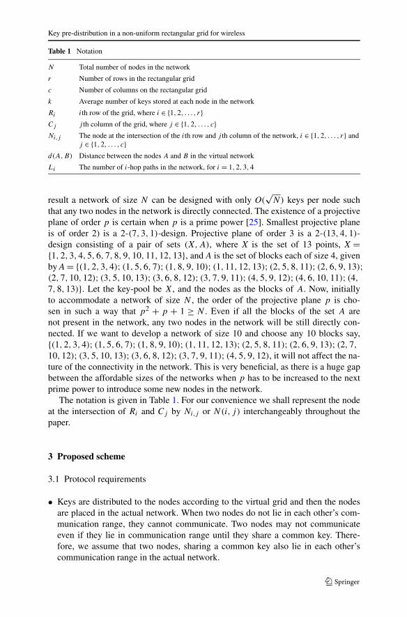
Table 1 Notation

N Total number of nodes in the network

r Number of rows in the rectangular grid

c Number of columns on the rectangular grid

k Average number of keys stored at each node in the network

Ri ith row of the grid, where i ∈ {1,2, . . . , r}Cj j th column of the grid, where j ∈ {1,2, . . . , c}Ni,j The node at the intersection of the ith row and j th column of the network, i ∈ {1,2, . . . , r} and

j ∈ {1,2, . . . , c}d(A,B) Distance between the nodes A and B in the virtual network

Li The number of i-hop paths in the network, for i = 1,2,3,4

result a network of size N can be designed with only O(√

N) keys per node suchthat any two nodes in the network is directly connected. The existence of a projectiveplane of order p is certain when p is a prime power [25]. Smallest projective planeis of order 2) is a 2-(7,3,1)-design. Projective plane of order 3 is a 2-(13,4,1)-design consisting of a pair of sets (X,A), where X is the set of 13 points, X ={1,2,3,4,5,6,7,8,9,10,11,12,13}, and A is the set of blocks each of size 4, givenby A = {(1,2,3,4); (1,5,6,7); (1,8,9,10); (1,11,12,13); (2,5,8,11); (2,6,9,13);(2,7,10,12); (3,5,10,13); (3,6,8,12); (3,7,9,11); (4,5,9,12); (4,6,10,11); (4,

7,8,13)}. Let the key-pool be X, and the nodes as the blocks of A. Now, initiallyto accommodate a network of size N , the order of the projective plane p is cho-sen in such a way that p2 + p + 1 ≥ N . Even if all the blocks of the set A arenot present in the network, any two nodes in the network will be still directly con-nected. If we want to develop a network of size 10 and choose any 10 blocks say,{(1,2,3,4); (1,5,6,7); (1,8,9,10); (1,11,12,13); (2,5,8,11); (2,6,9,13); (2,7,

10,12); (3,5,10,13); (3,6,8,12); (3,7,9,11); (4,5,9,12), it will not affect the na-ture of the connectivity in the network. This is very beneficial, as there is a huge gapbetween the affordable sizes of the networks when p has to be increased to the nextprime power to introduce some new nodes in the network.

The notation is given in Table 1. For our convenience we shall represent the nodeat the intersection of Ri and Cj by Ni,j or N(i, j) interchangeably throughout thepaper.

3 Proposed scheme

3.1 Protocol requirements

• Keys are distributed to the nodes according to the virtual grid and then the nodesare placed in the actual network. When two nodes do not lie in each other’s com-munication range, they cannot communicate. Two nodes may not communicateeven if they lie in communication range until they share a common key. There-fore, we assume that two nodes, sharing a common key also lie in each other’scommunication range in the actual network.

S. Mitra et al.

• We consider random node capture attack as the adversarial model through the pa-per. Under this attack the adversary captures a few nodes from the network atrandom and extracts all the keys stored at them.

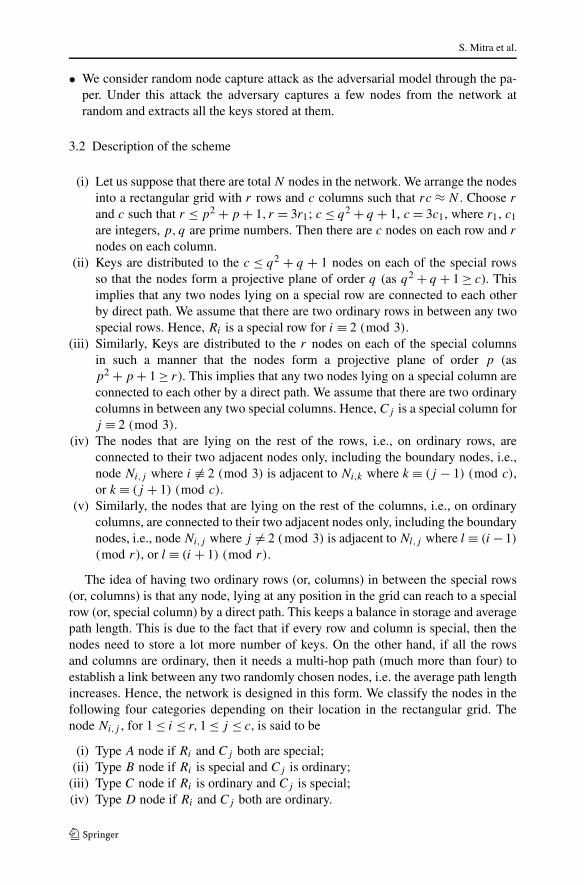
3.2 Description of the scheme

(i) Let us suppose that there are total N nodes in the network. We arrange the nodesinto a rectangular grid with r rows and c columns such that rc ≈ N . Choose r

and c such that r ≤ p2 + p + 1, r = 3r1; c ≤ q2 + q + 1, c = 3c1, where r1, c1

are integers, p,q are prime numbers. Then there are c nodes on each row and r

nodes on each column.(ii) Keys are distributed to the c ≤ q2 + q + 1 nodes on each of the special rows

so that the nodes form a projective plane of order q (as q2 + q + 1 ≥ c). Thisimplies that any two nodes lying on a special row are connected to each otherby direct path. We assume that there are two ordinary rows in between any twospecial rows. Hence, Ri is a special row for i ≡ 2 (mod 3).

(iii) Similarly, Keys are distributed to the r nodes on each of the special columnsin such a manner that the nodes form a projective plane of order p (asp2 + p + 1 ≥ r). This implies that any two nodes lying on a special column areconnected to each other by a direct path. We assume that there are two ordinarycolumns in between any two special columns. Hence, Cj is a special column forj ≡ 2 (mod 3).

(iv) The nodes that are lying on the rest of the rows, i.e., on ordinary rows, areconnected to their two adjacent nodes only, including the boundary nodes, i.e.,node Ni,j where i �≡ 2 (mod 3) is adjacent to Ni,k where k ≡ (j − 1) (mod c),or k ≡ (j + 1) (mod c).

(v) Similarly, the nodes that are lying on the rest of the columns, i.e., on ordinarycolumns, are connected to their two adjacent nodes only, including the boundarynodes, i.e., node Ni,j where j �= 2 (mod 3) is adjacent to Nl,j where l ≡ (i − 1)

(mod r), or l ≡ (i + 1) (mod r).

The idea of having two ordinary rows (or, columns) in between the special rows(or, columns) is that any node, lying at any position in the grid can reach to a specialrow (or, special column) by a direct path. This keeps a balance in storage and averagepath length. This is due to the fact that if every row and column is special, then thenodes need to store a lot more number of keys. On the other hand, if all the rowsand columns are ordinary, then it needs a multi-hop path (much more than four) toestablish a link between any two randomly chosen nodes, i.e. the average path lengthincreases. Hence, the network is designed in this form. We classify the nodes in thefollowing four categories depending on their location in the rectangular grid. Thenode Ni,j , for 1 ≤ i ≤ r,1 ≤ j ≤ c, is said to be

(i) Type A node if Ri and Cj both are special;(ii) Type B node if Ri is special and Cj is ordinary;

(iii) Type C node if Ri is ordinary and Cj is special;(iv) Type D node if Ri and Cj both are ordinary.

Key pre-distribution in a non-uniform rectangular grid for wireless

Thus, the network is heterogeneous in nature, consisting of four types of nodes. Wefurther assume that memory, transmission and computation capabilities of Type Anodes are the most, Type D nodes are least and Type B and Type C nodes are medium.

3.3 Deployment strategy

After the keys are loaded to the nodes according to the virtual network, nodes aredeployed in the target area to form the actual network. The following deploymentstrategy allows the actual network to match very close to the virtual network.

• In the first step, the set of nodes {N2,1,N2,2, . . . ,N2,c}, i.e., the nodes forming thespecial row R2 are deployed together.

• In the next step, the set of nodes {N1,2,N3,2,N4,2, . . . ,Nr,2}, i.e., the remainingnodes lying on the special column C2 are deployed together.

• Next, the sets of nodes {N5,1,N5,3,N5,4, . . . ,N5,c} forming special row R5 and{N1,5,N3,5,N4,5,N6,5,N7,5, . . . ,Nr,5} lying on the special column C5 are de-ployed one by one.

The process is repeated until all the nodes lying on a special row/column in the vir-tual grid are deployed. This way, if not all the nodes, then majority of the nodes ona special row/column will lie within each other’s transmission range. After the spe-cial rows and columns are taken care of, rest of the nodes on the ordinary rows andcolumns are deployed one by one. This is done because the special rows/columns aremore significant than the ordinary rows/columns.

4 Analysis

Theorem 4.1 The total number of one hop paths in the network is given by L1 =16 rc(r + c + 6).

Proof It follows from our construction that the key-pools for rows and columnsare disjoint. Hence we have the following disjoint cases considering row-wise andcolumn-wise communications.

(i) All nodes on a special row are connected to each other by one hop path.On the row Ri , Ni,j is connected by one hop paths to the nodes Ni,j ′ , forj ′ = {1,2, . . . , c} \ j , i.e., there are

(c2

)pairs (j, j ′) in Ri , for all i ≡ 2 (mod 3).

Therefore, number of one hop paths along all the special rows is r3

(c2

) =rc(c − 1)/6.

(ii) Similarly, on each special column Cj , any node Ni,j is connected by one hoppaths to the remanding r −1 nodes Ni′,j on the column, for i′ = {1,2, . . . , r} \ i.This implies, there are

(r2

)pairs (i, i′) in Cj , for all j ≡ 2 (mod 3). Hence total

number of one hop paths along the special columns is c3

(r2

) = rc(r − 1)/6.(iii) Any node Ni,j is connected by one hop paths to the nodes

• Ni−1,j and Ni+1,j on Cj when j �≡ 2 (mod 3) and• Ni,j−1 and Ni,j+1 on Ri when i �≡ 2 (mod 3)

S. Mitra et al.

Fig. 1 Multi-hop paths from aType A node

Fig. 2 Multi-hop paths from aType B node

Hence there are r and c one hop paths on each ordinary column and each ordi-nary row respectively (since, r ≥ 3, c ≥ 3). Hence the number of one-hop pathsunder this case is r 2c

3 + c 2r3 = 4rc

3 .

Thus, total number of single-hop paths in the network L1 = rc6 (c − 1) + rc

6 (r − 1) +4rc3 = 1

6 rc(r + c + 6). �

The multihop paths to all the remaining rc−1 nodes in the network from a Type A,Type B , Type C or a Type D node Ni,j are shown in Figs. 1, 2, 3 and 4 respectively.The node Ni,j is connected to the nodes, by 1-hop, 2-hop or 3-hop paths, marked bysquares, circles and diamonds respectively i n each of the figures. Ni,j is connectedto the nodes, marked by triangles in Fig. 4, by 4-hop paths.

Theorem 4.2 The total number of 2-hop paths in the network is L2 = 1954 rc(r + c) +

rc18 + 17

162 r2c2.

Key pre-distribution in a non-uniform rectangular grid for wireless

Fig. 3 Multi-hop paths from aType C node

Fig. 4 Multi-hop paths from aType D node

Proof Let L2A, L2B , L2C and L2D respectively denote the number of 2-hop pathsfrom a Type A, Type B , Type C and Type D node Ni,j . The ratio of these four typesof nodes is 1 : 2 : 2 : 4, hence we have L2 = 1

2 ( 19L2A + 2

9L2B + 29L2C + 4

9L2D).The factor 1

2 is appeared as each path is counted twice, corresponding to its twoends. In the following four cases we find the expressions for L2A, L2B , L2C andL2D , substituting these values in the above equation we obtain the desired expressionof L2.

(i) Expression for L2A The node Ni,j is key-connected in 2-hop paths to the follow-ing

Subcase(a) Ni−1,k and Ni+1,k , for k = {1,2, . . . , c}\{j}Subcase(b) Nl,j−1 and Nl,j+1, for l = {1,2, . . . , r}\{i − 1, i, i + 1}Subcase(c) Nl,k where Ck, k �= j is a special column; l = {1,2, . . . , r}\

{i − 1, i, i + 1}Subcase(d) Nl,k where l = {2x + 3 : 0 ≤ x ≤ r1} \ {i}; k = {1,2, . . . , c}\

{{j − 1, j, j + 1} ∪ {2y + 3 : 0 ≤ y ≤ c1}}

S. Mitra et al.

From the above discussion, we have 2(c − 1), 2(r − 3), 13 (r − 3)(c − 3) and

23 (r − 3)(c − 3) number of paths in Subcase (a), (b), (c) and (d) respectively.Summation of all these will lead to give an expression for L2A as L2A = 2(c −1)+2(r −3)+ 1

3 (r −3)(c−3)+ 29 (r −3)(c−3) = 2(r +c−4)+ 5

9 (r −3)(c−3).All these nodes are marked by circles in Fig. 1.

(ii) Expression for L2B The node Ni,j is key-connected in 2-hop paths to the follow-ing

Subcase(a) Ni−1,k and Ni+1,k , for k = {1,2, . . . , c}\{j}Subcase(b) Nl,k where Ck is a special column and l = {1,2, . . . , r}\{i − 1, i,

i + 1}Subcase(c) Ni+2,j and Ni−2,j

Above discussion implies that there are 2(c − 1), c(r − 3)/3 and 2 paths in Sub-case (a), (b) and (c) respectively. All of these will add to provide an expressionfor L2B as L2A = 2(c − 1) + c

3 (r − 3) + 2 = c3 (r + 3). Circles in Fig. 2 indicate

all these nodes.(iii) Expression for L2C The node Ni,j is key-connected in 2-hop paths to the fol-

lowing

Subcase(a) Nl,j−1 and Nl,j+1, for l = {1,2, . . . , r}\{i}Subcase(b) Nl,k where Rl is a special row and k = {1,2, . . . , c}\{j −1, j, j +1}Subcase(c) Ni,j+2 and Ni,j−2

Hence, it follows that there are 2(r − 1) , r(c − 3)/3 and 2 paths in Subcase (a),(b) and (c) respectively. Adding the above we obtain an expression for L2C asL2C = 2(r − 1) + r

3 (c − 3) + 2 = r3 (c + 3). All these nodes are shown as the

circles in Fig. 3.(iv) Expression for L2D The node Ni,j is key-connected in 2-hop paths to the fol-

lowing

Subcase(a) We note that if j ≡ 1 (mod 3), then Cj+1 is the nearest specialcolumn and when j ≡ 0 (mod 3), then Cj−1 is the nearest special column.In either cases, Ni,j is connected to nodes Nl,k where l = {1,2, . . . , r}\{i}and Ck is the special column nearest to Ni,j . Thus, the Type D is connectedto r − 1 nodes on its nearest special column.

Subcase(b) Similarly, if i ≡ 1 (mod 3), then Ri+1 is the nearest special rowand when i ≡ 0 (mod 3), then Ri−1 is the nearest special row. In eithercases, Ni,j is connected to nodes Nl,k′ where k = {1,2, . . . , c}\{i, k′}, Rl isthe special row and Ck′ is the special column respectively, nearest to Ni,j .Thus, the Type D is connected to c − 2 nodes on its nearest special row.

Subcase(c) Ni+2,j and Ni−2,j

Subcase(d) Ni,j+2 and Ni,j−2

Hence, The required expression is L2D = (r − 1) + (c − 2) + 4 = (r + c + 1).Circles in Fig. 4 denote these nodes.

Substituting the values and simplifying we obtain the final expression L2 = 1954 rc(r +

c) + rc18 + 17

162 r2c2. �

Key pre-distribution in a non-uniform rectangular grid for wireless

Theorem 4.3 The total number of 3-hop paths in the network is L3 = 29 rc( 4

3 rc− r −c − 11).

Proof We proceed in the similar manner as the proof of the previous theorem in thiscase. Here, we assume that L3A, L3B , L3C and L3D represents the number of 3-hoppaths from a Type A, Type B , Type C and Type D node Ni,j respectively. Now,we have L3 = 1

2 ( 19L3A + 2

9L3B + 29L3C + 4

9L3D). As already mentioned, the factor12 comes in since each path is counted twice, corresponding to its two ends. In thefollowing four cases we compute L3A, L3B , L3C and L3D , substituting these valuesin the above equation we obtain the desired expression of L3.

(i) Expression for L3A Note that a Type A node is connected to all Type B andType C nodes by 2-hop paths. Hence the connections to Type B and Type C

nodes in this case are ruled out. Moreover, a Type A node Ni,j is also connectedto the Type D nodes lying on the rows Ri−1, Ri+1 and the columns Cj+1 andCj−1 by 2-hop path. From Fig. 1 we can notice that there are no 4-hop path froma Type A node. Therefore, the nodes that lie on the intersection of the remainingr − r1 − 2 rows and c − c1 − 2 columns are connected to by a 3-hop path, asmarked by diamonds in Fig. 1. Thus, L3A = 4

9 (r − 3)(c − 3).(ii) Expression for L3B From Fig. 2 we observe that Type B node is connected to all

the Type C nodes and all the Type D nodes lying on the rows Ri−1, Ri+1, andtwo more Type D nodes Ni+2,j and Ni−2,j lying on the column Cj by a 2-hoppaths. Ni,j is connected to all the nodes on the row Ri and the nodes Ni+1,j andNi−1,j lying on the column Cj by 1-hop path. As there are no 4-hop path froma Type B node, all the remaining nodes are connected to Ni,j by a 3-hop path asindicated by in Fig. 2. Thus, L3B = 2

3 (2c − 3) + 2c3 (r − 5) = 2

3 (rc − 3c − 3).(iii) Expression for L3C Similarly as the previous case we find that a Type C node

is connected to all the Type B nodes and all the Type D nodes lying on thecolumns Cj−1, Cj+1, and two more Type D nodes Ni,j+2 and Ni,j−2 lying onthe row Ri by a 2-hop path. Ni,j is connected to all the nodes on the column Cj

and the nodes Ni,j+1 and Ni,j−1 lying on the column Cj by 1-hop path. Again,there are no 4-hop path from a Type C node, which can be verified from Fig. 3,all the remaining nodes are connected to Ni,j by a 3-hop path. These nodesare highlighted by diamonds in Fig. 3. Thus, L3C = 2

3 (2r − 3) + 2r3 (c − 5) =

23 (rc − 3r − 3).

(iv) Expression for L3D The node Ni,j is key-connected in 3-hop paths to the fol-lowing nodes

Subcase(a) Ni,k where k = {1,2, . . . , c}\{j − 2, j − 1, j, j + 1, j + 2}.Subcase(b) Nl,k for

l ={

i − 1, if i ≡ 1 (mod 3)

i + 1, if i ≡ 0 (mod 3)and k �=

{j + 1, if j ≡ 1 (mod 3)

j − 1, if j ≡ 0 (mod 3)

where Ck is a special columnSubcase(c) Nl,k where |l − i| = 2 and

k ={ {1,2, . . . , c}\{j, j + 1}, if j ≡ 1 (mod 3)

{1,2, . . . , c}\{j, j − 1}, if j ≡ 0 (mod 3)

S. Mitra et al.

Subcase(d) Nl,k where Rl is a special row, |l − i| ≥ 2 and

k ={ {1,2, . . . , c}\{j + 1}, if j ≡ 1 (mod 3)

{1,2, . . . , c}\{j − 1}, if j ≡ 0 (mod 3)

Subcase(e) Nl,k where Rl is not a special row,

l �={ {i − 1, i, i + 2}, if i ≡ 1 (mod 3)

{i − 2, i, i + 1}, if i ≡ 0 (mod 3)

and Ck is a special column but

k �={

j + 1, if j ≡ 1 (mod 3)

j − 1, if j ≡ 0 (mod 3)

Subcase(f) Nl,j where Rl is not a special row and l �= {i − 2, i, i + 2}Subcase(g) Nl,k where Rl is not a special row,

l �={ {i, i + 2}, if i ≡ 1 (mod 3)

{i − 2, i}, if i ≡ 0 (mod 3)

and

k ={

j + 2, if j ≡ 1 (mod 3)

j − 2, if j ≡ 0 (mod 3).

From the above discussion, we get (c − 5), ( c3 − 1), 2(c − 2), ( r

3 − 2)(c − 1),( c

3 − 1)( 2r3 − 3), ( 2r

3 − 3) and ( 2r3 − 2) number of paths in Subcase (a), (b), (c)

(d), (e), (f) and (g) respectively. Adding all the seven expressions obtained weget L3D = 5

9 rc + r3 + c

3 − 10. These nodes are indicated by diamonds in Fig. 4.

Substituting the values and simplifying we obtain the final expression as L3 =29 rc( 4

3 rc − r − c − 11). �

Theorem 4.4 The total number of 4-hop paths in the network is given by L3 =881 rc(rc − 3r − 3c + 9).

Proof Let us assume that L4A, L4B , L4C and L4D represent the number of 4-hoppaths from a Type A, Type B , Type C and Type D node Ni,j respectively. Now, wehave L4 = 1

2 ( 19L4A + 2

9L4B + 29L4C + 4

9L4D), since the ratio of four types of nodes inthe network is 1 : 2 : 2 : 4. As already mentioned, the factor 1

2 appears since each pathis counted twice, corresponding to its two ends. From Figs. 1–4, it is observed that aType A, Type B or a Type C node is connected to all the nodes by a path of maximumlength three. Hence, L4A = L4B = L4C = 0. A 4-hop path can be observed betweentwo Type D nodes as shown in Fig. 4. Proceeding in the similar manner as above weobtain L4D = 4

9 (r −3)(c−3). Now, L4 = 12 (L4ANA +L4BNB +L4CNC +L4DND)

give L4 = 881 rc(rc − 3r − 3c + 9). �

The average path length between any two nodes in the block graph of the networkis d = L1+2L2+3L3+4L4

L1+L2+L3+L4.

Key pre-distribution in a non-uniform rectangular grid for wireless

4.1 KeyPath establishment

Let us consider that two nodes N1(i1, j1) and N2(i2, j2) wish to communicate witheach other. We consider the following cases

Case 1: Let

i1 ≡ 2 (mod 3), j1 ≡ 2 (mod 3), i.e.,N1(i1, j1) is a Type A node;i2 ≡ 2 (mod 3), j2 ≡ 2 (mod 3), i.e.,N2(i2, j2) is a Type A node.

If i1 = i2 or j1 = j2 then the two communicating nodes are directly connected;otherwise the intermediate node between N1(i1, j1) and N2(i2, j2) is N(i1, j2) orN(i2, j1).

Case 2: Let

i1 ≡ 2 (mod 3), j1 ≡ 2 (mod 3), i.e.,N1(i1, j1) is a Type A node;i2 ≡ 2 (mod 3), j2 �≡ 2 (mod 3), i.e.,N2(i2, j2) is a Type B node.

If i1 = i2 then the two communicating nodes are directly connected; otherwise theintermediate node between N1(i1, j1) and N2(i2, j2) is N(i2, j1).

Case 3: Let

i1 ≡ 2 (mod 3), j1 ≡ 2 (mod 3), i.e.,N1(i1, j1) is a Type A node;i2 �≡ 2 (mod 3), j2 ≡ 2 (mod 3), i.e.,N2(i2, j2) is a Type C node.

If j1 = j2, then the two communicating nodes are directly connected; otherwise theintermediate node between N1(i1, j1) and N2(i2, j2) is N(i1, j2).

Case 4: Let

i1 ≡ 2 (mod 3), j1 ≡ 2 (mod 3), i.e.,N1(i1, j1) is a Type A node;i2 �≡ 2 (mod 3), j2 �≡ 2 (mod 3), i.e.,N2(i2, j2) is a Type D node.

• If |j1 − j2| = 1 then N(i2, j1) is an intermediate node between them.else if j2 ≡ 1 (mod 3), then the 3-hop key path is N1(i1, j1) → N(i1, j2 + 1) →N(i2, j2 + 1) → N2(i2, j2)

else j2 ≡ 0 (mod 3), then the 3-hop key path is N1(i1, j1) → N(i1, j2 − 1) →N(i2, j2 − 1) → N2(i2, j2)

• If |i1 − i2| = 1 then N(i1, j2) is an intermediate node between them.else if i2 ≡ 1 (mod 3), then the 3-hop key path is N1(i1, j1) → N(i2 + 1, j1) →N(i2 + 1, j2) → N2(i2, j2)

else i2 ≡ 0 (mod 3), then the 3-hop key path is N1(i1, j1) → N(i2 − 1, j1) →N(i2 − 1, j2) → N2(i2, j2).

Case 5: Let

i1 ≡ 2 (mod 3), j1 �≡ 2 (mod 3), i.e.,N1(i1, j1) is a Type B node;i2 ≡ 2 (mod 3), j2 �≡ 2 (mod 3), i.e.,N2(i2, j2) is a Type B node.

S. Mitra et al.

If i1 = i2 then the two communicating nodes are directly connectedelse if j2 ≡ 0 (mod 3), then the 3-hop key path is N1(i1, j1) → N(i1, j2 − 1) →N(i2, j2 − 1) → N2(i2, j2)

else j2 ≡ 1 (mod 3), then the 3-hop key path is N1(i1, j1) → N(i1, j2 + 1) →N(i2, j2 + 1) → N2(i2, j2).

Case 6: Let

i1 ≡ 2 (mod 3), j1 �≡ 2 (mod 3), i.e.,N1(i1, j1) is a Type B node;i2 �≡ 2 (mod 3), j2 ≡ 2 (mod 3), i.e.,N2(i2, j2) is a Type C node.

The he intermediate node between N1(i1, j1) and N2(i2, j2) is N(i1, j2).Case 7: Let

i1 ≡ 2 (mod 3), j1 �≡ 2 (mod 3), i.e.,N1(i1, j1) is a Type B node;i2 �≡ 2 (mod 3), j2 �≡ 2 (mod 3), i.e.,N2(i2, j2) is a Type D node.

If j1 = j2 and |i1 − i2| ≤ 2, then the key path is the straight line segment betweenN1 and N2 (1-hop or 2-hop) along the column Cj2 .else if j2 ≡ 0 (mod 3), then the 3-hop key path is N1(i1, j1) → N(i1, j2 − 1) →N(i2, j2 − 1) → N2(i2, j2)

else j2 ≡ 1 (mod 3), then the 3-hop key path is N1(i1, j1) → N(i1, j2 + 1) →N(i2, j2 + 1) → N2(i2, j2).

Case 8: Let

i1 �≡ 2 (mod 3), j1 ≡ 2 (mod 3), i.e.,N1(i1, j1) is a Type C node;i2 �≡ 2 (mod 3), j2 ≡ 2 (mod 3), i.e.,N2(i2, j2) is a Type C node.

If j1 = j2, then the two communicating nodes are directly connected;else if i2 ≡ 1 (mod 3), then the 3-hop key path is N1(i1, j1) → N(i2 + 1, j1) →N(i2 + 1, j2) → N2(i2, j2)

else i2 ≡ 0 (mod 3), then the 3-hop key path is N1(i1, j1) → N(i2 − 1, j1) →N(i2 − 1, j2) → N2(i2, j2).

Case 9: Let

i1 �≡ 2 (mod 3), j1 ≡ 2 (mod 3), i.e.,N1(i1, j1) is a Type C node;i2 �≡ 2 (mod 3), j2 �≡ 2 (mod 3), i.e.,N2(i2, j2) is a Type D node.

If i1 = i2 and |j1 − j2| ≤ 2, then the key path is the straight line segment betweenN1 and N2 (1-hop or 2-hop) along the row Ri2 .else if i2 ≡ 1 (mod 3), then the 3-hop key path is N1(i1, j1) → N(i2 + 1, j1) →N(i2 + 1, j2) → N2(i2, j2)

else i2 ≡ 0 (mod 3), then the 3-hop key path is N1(i1, j1) → N(i2 − 1, j1) →N(i2 − 1, j2) → N2(i2, j2).

Case 10: Let

i1 �≡ 2 (mod 3), j1 �≡ 2 (mod 3), i.e.,N1(i1, j1) is a Type D node;i2 �≡ 2(mod 3), j2 �≡ 2 (mod 3), i.e.,N2(i2, j2) is a Type D node.

Key pre-distribution in a non-uniform rectangular grid for wireless

If j1 ≡ 1 (mod 3)

if i2 ≡ 1 (mod 3) the 4-hop key path is given by N1(i1, j1) → N(i1, j1 + 1) →N(i2 + 1, j1 + 1) → N(i2 + 1, j2) → N2(i2, j2)

else if i2 ≡ 0 (mod 3) the 4-hop key path is given by N1(i1, j1) → N(i1,

j1 + 1) → N(i2 − 1, j1 + 1) → N(i2 − 1, j2) → N2(i2, j2)

else if j1 ≡ 0 (mod 3)

if i2 ≡ 1 (mod 3) the 4-hop key path is given by N1(i1, j1) → N(i1, j1 − 1) →N(i2 + 1, j1 − 1) → N(i2 + 1, j2) → N2(i2, j2)

else if i2 ≡ 0 (mod 3) the 4-hop key path is given by N1(i1, j1) → N(i1,

j1 − 1) → N(i2 − 1, j1 − 1) → N(i2 − 1, j2) → N2(i2, j2).

5 Performance

In this section we evaluate the efficiency of our scheme on the basis of connectivity,resilience and memory. For convenient comparison, we consider network consistingof nearly 2000 nodes. We further consider fifteen sets of combinations of the numberof rows and columns which lead to network of size almost 2000. We carry out all thecomputations and comparisons with these fifteen sets of values.

5.1 Memory

We note that the number of keys to be stored by a node depends on the Type of thatnode. Let us assume that kA, kB , kC and kD denote the number of keys to be storedby a Type A, Type B , Type C and Type D nodes respectively. Let us suppose that k

represents the average memory of any node i.e., average number of keys to be storedby each node from the network. It can also be observed that kD is independent of thechoices of the number of rows and number of columns present in the network andkD = 4 always.

In Table 2 we show the memory requirements of a network composed of more orless 2000 nodes, with different choice of the number of rows and columns, as statedearlier. From the table it is evident that the memory requirement is very small in ournetwork: a node needs to store a minimum of 8 keys to a maximum of 13 keys. Itcan also be noted from Table 2 that the deviation in storage is not much and does notfollow any strict pattern (increasing or decreasing), with increasing number of rows.Overall, it can be observed that if there is a huge difference in the number of rows,and columns, storage becomes comparatively more.

5.2 Connectivity

The percentage of one-hop, two-hop, 3-hop and 4-hop paths denoted by l1, l2, l3and l4 respectively, and the average path length d between any two randomly chosennodes, corresponding to each of the fifteen sets are listed in Table 3. From the tablewe note that the best possible case is achieved when the number of rows is verysmall, and the number of columns is very large or vice-versa (since the network issymmetric in rows and columns). In this case, there is no 4-hop path and the numberof one-hop and 2-hop paths are more in percentage as compared to other cases. As anobvious consequence, the average path length d is minimum in this case.

S. Mitra et al.

Table 2 Memoryr p c q kA kB kC k

3 2 666 27 31 30 5 13

6 2 333 19 23 22 5 ≤11

9 3 222 16 21 19 6 ≤10

12 3 168 13 18 16 6 ≤9

15 4 135 11 17 14 7 ≤9

18 4 111 11 17 14 7 ≤9

21 4 96 11 17 14 7 ≤9

24 5 81 9 16 12 8 8

27 5 75 9 16 12 8 8

30 5 69 8 15 11 8 ≤8

33 7 63 8 17 11 10 ≤9

36 7 57 7 16 10 10 8

39 7 41 7 16 10 10 8

42 7 48 7 16 10 10 8

45 7 45 7 16 10 10 8

Table 3 Connectivity

r c l1 l2 l3 l4 d

3 666 11.266900 44.577976 44.155121 0 2.328882

6 333 5.758638 32.949425 51.499470 9.792466 2.653258

9 222 3.955934 29.143715 53.903076 12.997273 2.759417

12 168 3.076923 27.289722 55.075821 14.557486 0.811139

15 135 2.569171 26.218676 55.753212 15.458944 2.841019

18 111 2.253380 25.549435 56.173149 16.024036 2.859679

21 96 2.034739 25.089605 56.465397 16.410257 2.872512

24 81 1.904272 24.806999 56.636360 16.652370 2.8880368

27 75 1.778657 24.549810 56.807232 16.864304 2.887572

30 69 1.691638 24.370335 56.924976 17.013050 2.892594

33 63 1.636189 24.254055 56.999279 17.110477 2.895840

36 57 1.608971 24.194160 57.034508 17.162359 2.897503

39 41 1.609659 24.189543 57.031105 17.169693 2.897608

42 48 1.588089 24.146677 57.060932 17.204302 2.898814

45 45 1.581028 24.132593 57.070736 17.215643 2.899210

5.3 Resilience

Sensor nodes are usually deployed in hostile region; therefore, they are liable of fre-quently getting captured by the adversary. We consider random node capture attackas the adversarial model, i.e., the adversary captures a number of nodes randomlyfrom the network and extracts all the keys stored at them. The rest of the networkwill not be able to make use of these keys any more, for communication. As a result,

Key pre-distribution in a non-uniform rectangular grid for wireless

the rest of the network, although not compromised, still gets affected. Resilience isthe measure to quantify the robustness of the network is against adversarial attack,i.e., when a few nodes are captured by the adversary, how well the rest of the networkcontinues to communicate with each other. Now, the effect of the adversarial attack istwo fold—on the nodes and the links. We discuss them in the following subsectionsin detail.

We estimate resilience for a network consisting of almost 2000 nodes. Note thatN = 2000 can be obtained with different pairs of (r, c) values where r is the numberof rows and c is the number of columns. We consider the same fifteen pairs of (r, c)

values (r = 3, c = 666) to (r = 45, c = 45) as used in Tables 2 and 3. Since thenetwork is symmetric in r and c, (r = 3, c = 666) is same as (r = 666, c = 3). Wecarry out all the computations considering these fifteen pairs of values throughoutthis section and try to find out the best possible cases.

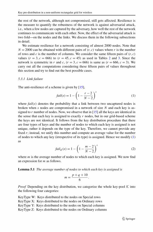
5.3.1 Link failure

The anti-resilience of a scheme is given by [15],

fail(s) = 1 −(

1 − r − 2

N − 2

)s

(1)

where fail(s) denotes the probability that a link between two uncaptured nodes isbroken when s nodes are compromised in a network of size N and each key is as-signed to r number of nodes. Now, we observe that in [15] all the keys are identical inthe sense that each key is assigned to exactly r nodes, but in our grid-based schemethe keys are not identical. It follows from the key distribution procedure that thereare four types of keys and the number of nodes to which each key is assigned is notunique, rather it depends on the type of the key. Therefore, we cannot provide anyfixed r ; instead, we unify this number and compute an average value for the numberof nodes to which any key (irrespective of its type) is assigned. Hence we modify (1)as

failE(s) = 1 −(

1 − m − 2

N − 2

)s

(2)

where m is the average number of nodes to which each key is assigned. We now findan expression for m as follows.

Lemma 5.1 The average number of nodes to which each key is assigned is

m = p + q + 10

6.

Proof Depending on the key distribution, we categorize the whole key-pool K intothe following four categories:

KeyType W: Keys distributed to the nodes on Special rowsKeyType X: Keys distributed to the nodes on Ordinary rowsKeyType Y: Keys distributed to the nodes on Special columnsKeyType Z: Keys distributed to the nodes on Ordinary columns

S. Mitra et al.

Let degγ be the total number of nodes to which a KeyType γ key is assigned andtotγ represents the total number of KeyType γ keys required for key distribution,where γ ∈ {W,X,Y,Z}. Hence,

m =∑

γ degγ totγ∑

γ totγ, γ ∈ {W,X,Y,Z}. (3)

Note that degW = q + 1,degX = 2,degY = p + 1,degZ = 2. Since each specialrow needs c = q2 + q + 1 keys and there are total r

3 special rows, we have totW =r3 (q2 + q + 1) ≈ rc

3 . Proceeding in similar manner and utilizing the symmetry of thenetwork, we obtain totX = 2rc/3, totY = rc/3 and totZ = 2rc/3. Substituting thesevalues in Eq. (3), we get

m =rc3 × (q + 1) + rc

3 × (p + 1) + 2rc3 × 2 + 2rc

3 × 2rc3 + rc

3 + 2rc3 + 2rc

3

= p + q + 10

6. (4)

�

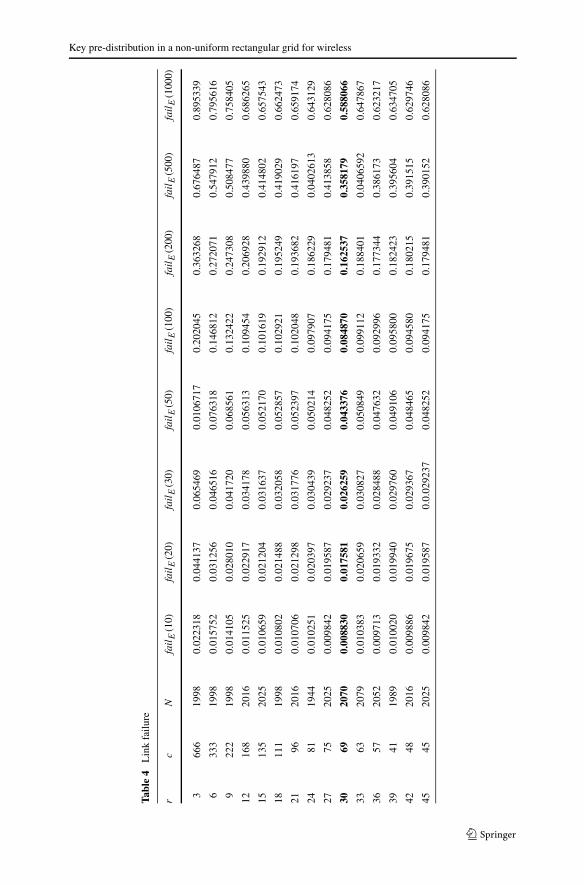
Table 4 corresponds to the link failure, i.e., failE(s) of Layout I. We obtainfailE(10) as the standard comparison measure in the literature, however, apartfrom failE(10) we also calculate failE(s) for a number of values of s, given by20,30,50,100,200,500 and 1000, which shows how the network catastrophicallybreaks down with a huge number of compromised nodes. We observe from the tablethat any particular pattern can not be obtained but the best case is achieved for r = 30and c = 69, which is highlighted.

Now, we compare the best possible cases obtained for the two measures of re-silience. The best case for node disconnection is achieved when N = 1998 withr = 3, c = 666, then failV (100) = 0.004053 and failE(10) = 0.022318.

5.3.2 Node disconnection

The expression for node disconnection is failV (s) which represents the fraction ofthe total number of nodes that become disconnected when s nodes are captured un-der adversarial attack. We assume failV (s) = v1(s)

N−s, where v1(s) denotes the average

number of nodes that becomes disconnected and N is the total number of nodes inthe network. We find an expression for v1(s) as follows.

Lemma 5.2 The average number of nodes, that become disconnected when s nodesare captured, is given by v1(s) = 3s

p+q+10 , where p,q are two prime powers satisfying

r ≤ p2 + p + 1, c ≤ q2 + q + 1.

Proof From the construction, we observe that the number of nodes to be compro-mised to disconnect one node from the network depends on the type of the node.Let vβ be the number of nodes to be compromised to disconnect a Type β node, forβ ∈ {A,B,C,D}. Now, the proportion of the four types of nodes are 1

9 , 29 , 2

9 and 49 .

Hence v1(s) = s19 vA+ 2

9 vB+ 29 vC+ 4

9 vD.

Key pre-distribution in a non-uniform rectangular grid for wireless

Tabl

e4

Lin

kfa

ilure

rc

Nfa

ilE

(10)

failE

(20)

failE

(30)

failE

(50)

failE

(100

)fa

ilE

(200

)fa

ilE

(500

)fa

ilE

(100

0)

366

619

980.

0223

180.

0441

370.

0654

690.

0106

717

0.20

2045

0.36

3268

0.67

6487

0.89

5339

633

319

980.

0157

520.

0312

560.

0465

160.

0763

180.

1468

120.

2720

710.

5479

120.

7956

16

922

219

980.

0141

050.

0280

100.

0417

200.

0685

610.

1324

220.

2473

080.

5084

770.

7584

05

1216

820

160.

0115

250.

0229

170.

0341

780.

0563

130.

1094

540.

2069

280.

4398

800.

6862

65

1513

520

250.

0106

590.

0212

040.

0316

370.

0521

700.

1016

190.

1929

120.

4148

020.

6575

43

1811

119

980.

0108

020.

0214

880.

0320

580.

0528

570.

1029

210.

1952

490.

4190

290.

6624

73

2196

2016

0.01

0706

0.02

1298

0.03

1776

0.05

2397

0.10

2048

0.19

3682

0.41

6197

0.65

9174

2481

1944

0.01

0251

0.02

0397

0.03

0439

0.05

0214

0.09

7907

0.18

6229

0.04

0261

30.

6431

29

2775

2025

0.00

9842

0.01

9587

0.02

9237

0.04

8252

0.09

4175

0.17

9481

0.41

3858

0.62

8086

3069

2070

0.00

8830

0.01

7581

0.02

6259

0.04

3376

0.08

4870

0.16

2537

0.35

8179

0.58

8066

3363

2079

0.01

0383

0.02

0659

0.03

0827

0.05

0849

0.09

9112

0.18

8401

0.04

0659

20.

6478

67

3657

2052

0.00

9713

0.01

9332

0.02

8488

0.04

7632

0.09

2996

0.17

7344

0.38

6173

0.62

3217

3941

1989

0.01

0020

0.01

9940

0.02

9760

0.04

9106

0.09

5800

0.18

2423

0.39

5604

0.63

4705

4248

2016

0.00

9886

0.01

9675

0.02

9367

0.04

8465

0.09

4580

0.18

0215

0.39

1515

0.62

9746

4545

2025

0.00

9842

0.01

9587

0.0.

0292

370.

0482

520.

0941

750.

1794

810.

3901

520.

6280

86

S. Mitra et al.

Table 5 Node disconnectionr p c q N failV (100) failV (150) failV (200)

3 2 666 27 1998 0.004053 0.006244 0.008557

6 2 333 19 1998 0.005099 0.007855 0.010765

9 3 222 16 1998 0.005450 0.008397 0.011507

12 3 168 13 2016 0.006022 0.009275 0.012708

15 4 135 11 2025 0.006234 0.009600 0.013151

18 4 111 11 1998 0.006322 0.009740 0.013348

21 4 96 11 2016 0.006263 0.009646 0.013216

24 5 81 9 1944 0.006779 0.010452 0.014335

27 5 75 9 2025 0.006494 0.010000 0.013699

30 5 69 8 2070 0.006621 0.010190 0.013950

33 7 63 8 2079 0.006064 0.009331 0.012773

36 7 57 7 2052 0.006404 0.009858 0.013499

39 7 41 7 1989 0.006617 0.010196 0.013974

42 7 48 7 2016 0.006524 0.010048 0.013767

45 7 45 7 2025 0.006494 0.010000 0.013699

To compute vA A Type A node N(i, j) is situated at the intersection of a specialrow Ri and a special column Cj . Each special row or special column gets a key-distribution according to a projective plane of order q or of order p respectively. Aswe have already mentioned earlier that to disconnect a Type A node N(i, j) fromthe network, at least q +1 nodes along the row Ri and p+1 nodes along the columnCj have to be captured. This gives vA = p + q + 2.

To compute vB A Type B node N(i, j) lies on a especial row Ri and an ordinarycolumn Cj . According to the above arguments, disconnect a Type B node N(i, j),both adjacent nodes N(i − 1, j), N(i+, j) along the column Cj and at least at leastq + 1 nodes along the row Ri should be captured. Hence, we get vB = q + 3.

Proceeding similarly we obtain that vC = p+3 and vD = 4. Substituting these valuesand simplifying we obtain the final expression as v1(s) = 3s

p+q+10 . �

Hence, as a consequence, the expression for node disconnection is given by

failV (s) = v1(s)

N − s= 3s

(p + q + 10)(N − s).

The values of failV (s) for the same fifteen pairs of (r, c) values are listed in Ta-ble 5, for three different values of s, viz. 100, 150 and 200, to match up with exist-ing works, as they have considered these values for node disconnection comparison.From the table we observe that the best possible case is achieved when there arevery small number of rows and very large number of columns and vice-versa (whichfollows from the symmetry of the layout).

5.4 Comparison with existing schemes

In this subsection we provide the comparison of the resilience of our scheme with ex-isting schemes. Since all the related works which have been in this context, have used

Key pre-distribution in a non-uniform rectangular grid for wireless

Fig. 5 Comparison of nodedisconnection

Fig. 6 Comparison of linkfailure

different parameters, it is not feasible to compare the resilience of our scheme withthe existing ones. Hence we show the comparison graphically keeping the networksize fixed.

Node disconnection was considered as a measure of resilience by Ruj and Royin [20]. The comparison of failV (s) of our KPS with Ruj and Roy’s SBIBD [21]PBIBD I and PBIBD II scheme [20] is given in Fig. 5, keeping the size of the net-work almost equal to 2000 for each of the cases. Figure 5 indicates that the proposednetwork shows better node disconnection than the existing schemes.

Figure 6 graphically shows the comparative link failure of the proposed schemeswith that of the following existing schemes: Eschenauer-Gligor Basic scheme [13],Lee-Stinson Linear scheme and Quadratic scheme [16], Camptepe-Yener scheme [6],Chakrabarti et al.’s probabilistic Merging scheme [7], Ruj-Roy’s PBIBD-I, PBIBD-II[19] and Bag-Ruj’s affine plane based scheme [2] for a network of size N ≈ 2000

S. Mitra et al.

and a small number of compromised nodes s. Figure 6 illustrates that our networkoutperforms the existing schemes when link failure is concerned.

6 Conclusion

We have proposed key pre-distribution scheme for rectangular grid networks consid-ering using projective planes and pairwise connectivity. Unlike most of the combina-torial design based schemes, the memory prerequisite in each sensor node is appre-ciably less. Further, we perceive that the proposed scheme shows enough flexibilityin the sense that the performance measures of the evaluation metrics discussed inthe paper, can be controlled with suitable choice of the number of rows and columnsin the grid. The induced network enables any two nodes to be connected by at leastone path of length less than or equal to four. Additionally, there are multiple paths be-tween any two nodes chosen randomly from the network. Our network aloes providesbetter resilience as compared to existing combinatorial design based schemes.

References

1. Bag, S.: Key predistribution in 3-dimensional grid-group deployment scheme. In: CNSA 2011. CCIS,vol. 196, pp. 302–319 (2011)

2. Bag, S., Ruj, S.: Key distributions in wireless sensor networks using finite affine plane. In: IEEEComputer Society. Workshop of International Conference on Advanced Information Networking andApplications, pp. 436–441 (2011)

3. Bag, S., Dhar, A., Sarkar, P.: 100 % connectivity for location aware code based KPD in clusteredWSN: merging blocks. In: ISC 2012. LNCS, vol. 7483, pp. 136–150 (2012)

4. Bala, S., Sharma, G., Verma, A.K.: Classification of symmetric key management schemes for wirelesssensor networks. Int. J. Secur. Appl. 7(2), 117–138 (2013)

5. Blackburn, S.R., Etizon, T., Martin, K.M., Paterson, M.B.: Efficient key pre-distribution for grid-basedwireless sensor networks. In: ICITS 2008, pp. 54–69 (2008)

6. Camptepe, S.A., Yener, B.: Combinatorial design of key distribution mechanisms for wireless sensornetworks. In: ESORICS, vol. 3193, pp. 293–308. Springer, Berlin (2004)

7. Chakrabarti, D., Maitra, S., Roy, B.: A key pre-distribution scheme for wireless sensor networks:merging blocks in combinatorial design. In: ISC. LNCS, vol. 3650, pp. 89–103. Springer, Berlin(2005)

8. Chakrabarti, D., Maitra, S., Roy, B.: Clique size in sensor networks with key predistribution based ontransversal design. Int. J. Distrib. Sens. Netw. 3–4, 345–354 (2005)

9. Chakrabarti, D., Maitra, S., Roy, B.: A hybrid design of key pre-distribution scheme for wirelesssensor networks. In: ICISS 2005. LNCS, vol. 3803, pp. 228–238 (2005)

10. Chan, H., Perrig, A., Song, D.X.: Random key predistribution schemes for sensor network. In: IEEESymposium on Security and Privacy, pp. 197–213 (2003)

11. Chen, C.Y., Chao, H.C.: A survey of key predistribution in wireless sensor networks. Secur. Commun.Netw. (2011)

12. Dong, J., Pei, D., Wang, X.: A key predistribution scheme based on 3-designs. In: Inscrypt 2007.LNCS, vol. 4990, pp. 81–92. Springer, Berlin (2008)

13. Eschenauer, L., Gligor, V.D.: A key-management scheme for distributed sensor networks. In: ACMCCS, pp. 41–47. ACM, New York (2002)

14. Lee, J., Stinson, D.R.: Deterministic key predistribution schemes for distributed sensor networks. In:SAC 2004. LNCS, vol. 3357, pp. 294–307 (2005)

15. Lee, J., Stinson, D.R.: A combinatorial approach to key predistribution for distributed sensor net-works. In: IEEE WCNC, pp. 1200–1205 (2005)

16. Lee, J., Stinson, D.R.: On the construction of practical key predistribution schemes for distributedsensor networks using combinatorial designs. ACM Trans. Inf. Syst. Secur. 11(2), 5:1–5:35 (2008)

Key pre-distribution in a non-uniform rectangular grid for wireless

17. Mitchell, C.J., Piper, F.: Key storage in sensor networks. Discrete Appl. Math. 21, 215–228 (1988)18. Paterson, M.B., Stinson, D.R.: A unified approach to combinatorial key predistribution schemes for

sensor networks. IACR Cryptol. ePrint Arch. 2011, 76 (2011)19. Ruj, S., Roy, B.: Key predistributions using partially balanced designs in wireless sensor networks.

In: ISPA. LNCS, vol. 4742, pp. 431–445. Springer, Berlin (2007)20. Ruj, S., Roy, B.: Key predistributions schemes using codes in wireless sensor networks. In: Inscrypt

2008. LNCS, vol. 5487, pp. 275–288 (2009)21. Ruj, S., Seberry, J., Roy, B.: Key predistribution schemes using block designs in wireless sensor

networks. Int. Conf. Comput. Sci. Eng. 2, 873–878 (2009)22. Ruj, S., Nayak, A., Stojmenovic, I.: Fully secure pairwise and triple key distributions in wireless

networks using combinatorial designs. In: IEEE INFOCOM, pp. 326–330 (2011)23. Sadi, M.S., Park, J.S., Kim, D.K.: Randomized grid based scheme for wireless sensor network. In:

ESAS 2005. LNCS, vol. 3813, pp. 91–101 (2005)24. Simonova, K., Ling, A.C.H., Wang, X.S.: Location-aware key predistribution scheme for wide area

wireless sensor networks. In: SASN’06, October 30 (2006)25. Stinson, D.R.: Combinatorial Designs: Constructions and Analysis. Springer, New York (2003)