Key aspects of stratospheric tracer modeling

HAL Id: hal-00301342https://hal.archives-ouvertes.fr/hal-00301342

Submitted on 6 Jun 2006

HAL is a multi-disciplinary open accessarchive for the deposit and dissemination of sci-entific research documents, whether they are pub-lished or not. The documents may come fromteaching and research institutions in France orabroad, or from public or private research centers.

L’archive ouverte pluridisciplinaire HAL, estdestinée au dépôt et à la diffusion de documentsscientifiques de niveau recherche, publiés ou non,émanant des établissements d’enseignement et derecherche français ou étrangers, des laboratoirespublics ou privés.

Key aspects of stratospheric tracer modelingB. Bregman, E. Meijer, R. Scheele

To cite this version:B. Bregman, E. Meijer, R. Scheele. Key aspects of stratospheric tracer modeling. AtmosphericChemistry and Physics Discussions, European Geosciences Union, 2006, 6 (3), pp.4375-4414. �hal-00301342�

https://hal.archives-ouvertes.fr/hal-00301342

https://hal.archives-ouvertes.fr

ACPD6, 4375–4414, 2006

Stratospheric tracermodeling key aspects

B. Bregman et al.

Title Page

Abstract Introduction

Conclusions References

Tables Figures

J I

J I

Back Close

Full Screen / Esc

Printer-friendly Version

Interactive Discussion

EGU

Atmos. Chem. Phys. Discuss., 6, 4375–4414, 2006www.atmos-chem-phys-discuss.net/6/4375/2006/© Author(s) 2006. This work is licensedunder a Creative Commons License.

AtmosphericChemistry

and PhysicsDiscussions

Key aspects of stratospheric tracermodelingB. Bregman, E. Meijer, and R. Scheele

Royal Netherlands Meteorological Institute, P.O. Box 201, 3730 AE, De Bilt, The Netherlands

Received: 3 February 2006 – Accepted: 7 March 2006 – Published: 6 June 2006

Correspondence to: B. Bregman ([email protected])

4375

http://www.atmos-chem-phys-discuss.net

http://www.atmos-chem-phys-discuss.net/6/4375/2006/acpd-6-4375-2006-print.pdf

http://www.atmos-chem-phys-discuss.net/6/4375/2006/acpd-6-4375-2006-discussion.html

http://www.copernicus.org/EGU/EGU.html

ACPD6, 4375–4414, 2006


B. Bregman et al.

Title Page



Tables Figures

J I

J I

Back Close

Full Screen / Esc



EGU

Abstract

This study describes key aspects of global chemistry-transport models and the impacton stratospheric tracer transport. We concentrate on global models that use assim-ilated winds from numerical weather predictions, but the results also apply to tracertransport in general circulation models. We examined grid resolution, numerical diffu-5

sion and dispersion of the winds fields, the meteorology update time intervals, updatefrequency, and time interpolation. For this study we applied the three-dimensionalchemistry-transport Tracer Model version 5 (TM5) and a trajectory model and per-formed several diagnoses focusing on different transport regimes. Covering differenttime and spatial scales, we examined (1) polar vortex dynamics during the Arctic winter,10

(2) the large-scale stratospheric meridional circulation, and (3) air parcel dispersion inthe tropical lower stratosphere. Tracer distributions inside the Arctic polar vortex showconsiderably worse agreement with observations when the model grid resolution in thepolar region is reduced to avoid numerical instability. Using time interpolated windsimprove the tracer distributions only marginally. Considerable improvement is found15

when the update frequency of the assimilated winds is increased from 6 to 3 h, both inthe large-scale tracer distribution and the polar regions. It further reduces in particularthe vertical dispersion of air parcels in the tropical lower stratosphere. The results inthis study demonstrates significant progress in the use of assimilated meteorology inchemistry-transport models, which is important for both short- and long-term integra-20

tions.

1 Introduction

Global three dimensional chemistry transport models (hereafter referred to as CTMs)driven by actual meteorology from numerical weather predictions are crucial for the in-terpretation of many observational data. The great advantage is the direct comparison25

with observations by their ability to utilize actual meteorology to drive the model trans-

4376





ACPD6, 4375–4414, 2006


B. Bregman et al.

Title Page



Tables Figures

J I

J I

Back Close

Full Screen / Esc



EGU

port. CTMs are thus ideally designed for detailed sensitivity studies of key processesimportant for climate, which would be computationally too expensive for Chemistry-Climate Models (CCMs). Major areas of interest are the polar regions, owing to theprevailing chemical ozone loss during winter and its sensitivity towards climate change,and the tropical region where the main entrance of air into the stratosphere is located5

(WMO, 2002). The ability of a direct comparison with observations also allows modelsensitivity studies to investigate basic model parameters, such as grid resolution andadvection schemes, but also the quality of the wind fluxes or vectors and the way themeteorological information is implemented in the CTM.

The impact of grid resolution on the atmospheric composition remains an important10

subject of discussion. Searle et al. (1998) show that a horizontal resolution of 3◦ issufficient to calculate polar chemical ozone loss, but Marchand et al. (2003) in con-trast found substantial differences after increasing their model resolution from 2◦×2◦ to1◦×1◦. Another model study also focused on the effect of spatial resolution in the polarregion by evaluating methane distributions (van den Broek et al., 2003). An important15

outcome was the significant overestimation of methane in the lower stratosphere atthe edge and inside the polar vortex. An increase of the horizontal grid resolution to1◦×1◦ gave negligible improvement and thus indicated very small sensitivity to horizon-tal resolution. This results support the conclusions from Searle et al. (1998), althoughthe conclusions here were based on long-lived tracer distributions. The results in this20

study however contrasts these findings.CTMs and CCMs suffer from numerical instability in regions of strong zonal winds

and relatively small grid cells. The most critical regions are located at the poles, inparticular during the winter, but also in the vicinity of storm tracks. Negative tracer masscan occur when the transport distance during one advection time step exceeds the size25

of the grid cell, the so-called Courant-Friedrichs-Lewy (CFL) criterion. Commonly, thisis avoided by reducing the grid resolution or by averaging the wind vectors or massfluxes, but its impact on tracer transport has sofar not been investigated.

An obvious solution would be to reduce the advection time step, but this would lead

4377





ACPD6, 4375–4414, 2006


B. Bregman et al.

Title Page



Tables Figures

J I

J I

Back Close

Full Screen / Esc



EGU

to excessively small time steps. To overcome this difficulty we introduced an iterationprocedure for tracer advection in the TM5 model with locally adjusted time steps (Krolet al., 2005). In Krol et al. (2005) the focus was on the troposphere. In this study wewill demonstrate the dramatic impact on the stratospheric tracer distribution.

The quality of the winds provided by the numerical weather predictions is another5

factor affecting tracer transport. The winds are subject to data assimilation within themodel prediction and are often referred to as Data Assimilation System or DAS winds(Schoeberl et al., 2002). The quality of particularly the stratospheric winds is affectedby the presence of spurious variability or “noise”, inherently introduced through the as-similation procedure, either through a lack of suitable observations or by inaccurate10

treatment of the model biases. This unwanted variability causes enhanced dispersionthat accumulates in time. Hence, the impact of dispersion increases with increasing dy-namic time scales. It may therefore not be a serious problem for the troposphere wherethe dynamic turnover times are relatively short. However, the stratospheric circulationcontains much longer time scales where spurious variability in DAS winds becomes15

very critical. One of the consequences is enhanced dispersion and an enforced large-scale stratospheric meridional circulation, causing tracer residence times to be con-siderably shorter than observed (Schoeberl et al., 2002; Douglass et al., 2003; Meijeret al., 2004). The most critical region is the tropical lower stratosphere, where the ma-jority of the air enters the stratosphere. Moreover, this is a very complicated region for20

data assimilation due to a lack of observations and because the atmosphere deviatesfrom geostrophical balance, which complicates proper treatment of model biases.

Meijer et al. (2004) and Scheele et al. (2005) show that the intensity of disper-sion in the DAS winds increases when the assimilation procedure is less accurateor less sophisticated. For example, the ECMWF utilizes three- and four-dimensional25

assimilation procedures (3DVAR and 4DVAR respectively). 4DVAR is a temporal ex-tension of 3DVAR, and thus more accurate but also computationally more expensive.A comprehensive description of the ECWMF assimilation procedures can be found athttp://www.ecmwf.int. A major difference is that 4DVAR produces physically more bal-

4378





http://www.ecmwf.int

ACPD6, 4375–4414, 2006


B. Bregman et al.

Title Page



Tables Figures

J I

J I

Back Close

Full Screen / Esc



EGU

anced winds for each model time step, due to the inclusion of time. Because of compu-tational expenses the long-term re-analyses (ERA40) has been performed with 3DVAR,while the operational data, analyses and forecasts (referred to as “Operational Data”or OD) are produced with 4DVAR. Comparing both data sets thus yields informationabout the impact of assimilation accuracy on tracer transport. Ozone is a useful tracer,5

since its distribution is very vulnerable to the strength of large-scale stratospheric circu-lation. Laat et al. (2006) and van Noije et al. (2004) show a very strong accumulationof ozone in the extra-tropical lower stratosphere when using ERA40 winds, resultingin significant overestimation compared to observations. When applying OD winds, theagreement becomes much better. Indeed, van Noije et al. (2004), Simmons et al.10

(2005) and Scheele et al. (2005) have shown that OD winds contain less dispersionthan ERA40 winds in the tropical lower stratosphere and provide more realistic extra-tropical downward ozone fluxes (van Noije et al., 2004) and more realistic stratosphericresidence times (Meijer et al., 2004). However, even with OD the circulation remainstoo strong (Laat et al., 2006), which has led to the practical decision to constrain strato-15

spheric ozone down to 100 hPa in the extra-tropics with ozone climatology (van Noijeet al., 2004) for the tropospheric multi-year IPCC chemistry-transport runs. Howeverfor coupled troposphere-stratosphere runs this solution is undesirable.

Recently, a comprehensive model intercomparison was performed with winds andtemperatures from a variety of data assimilation systems, focusing on the 2002 Antarc-20

tic vortex split (Manney et al., 2005). They show substantial differences between themodels that apply different DAS, with operational (4DVAR) analysis performing betterthan re-analysis (3DVAR) data, consistent with the studies described above.

Despite shortcomings in ERA40 winds, the dynamical variability can be simulatedquite well (Hadjinicolaou et al., 2005; Chipperfield, 2006). This is in line with a compar-25

ison between DAS winds from different numerical weather predictions, where ERA40winds were found to agree excellent with observed variability (Randel et al., 2003). Itis important to note that instantaneous variability and enhanced dispersion or noise inthe winds are two separated issues. The above mentioned studies with ERA40 clearly

4379





ACPD6, 4375–4414, 2006


B. Bregman et al.

Title Page



Tables Figures

J I

J I

Back Close

Full Screen / Esc



EGU

demonstrate this.Recently, we have evaluated forecasts instead of analyses, assuming that forecasts

are physically more balanced and thus are expected to contain less noisy winds, similarto the differences between 3DVAR and 4DVAR winds. Indeed, in a recent trajectorystudy we have shown that by increasing the forecast length the dispersion in the tropical5

lower stratosphere is significantly reduced (Scheele et al., 2005). In line with theseresults the mean age of air becomes older in the extra-tropical stratosphere, closer toobservations (Meijer et al., 2004). However, it now became too old in the tropical lowerstratosphere, while still remaining too young in the extra-tropics.

The representation of the large-scale meridional circulation in the stratosphere by10

DAS winds considerably improves when using isentropic vertical coordinates and heat-ing rates instead of vertical wind velocity or mass fluxes on pressure levels (Mahowaldet al., 2002). Although an isentropic coordinate seems physically more appropriate forstratospheric dynamics, a mass correction needs to be performed in order to balancethe divergence with the isentrope tendencies, which will impact the tracer distributions.15

This is a fundamental mass balance problem that applies to both CTMs and GCMsindependent of the vertical coordinate system, as has been demonstrated by Jockelet al. (2001) and for which different mass fixers have been introduced (cf. Bregmanet al., 2003; Rotman et al., 2004). When integrating over a full vertical range from theupper stratosphere to the surface, the isentropic vertical coordinate needs to be ad-20

justed from purely isentropic to a hybrid of pressure and isentropes. So far only twomodels have inferred such a hybrid coordinate (Mahowald et al., 2002; Chipperfield,2006), which still contain mass imbalance issues but are promising developments.

By applying the algorithm of Segers et al. (2002), Bregman et al. (2003) have shownthat the use of mass fixers can be avoided by applying mass-flux advection, without25

violating mass conservation. This is a fundamental underlying aspect in this study.We have demonstrated complete mass conservation using the hybrid sigma-pressurecoordinate, while sofar this has not been proven for other vertical coordinate systems.

Hybrid sigma-pressure remains a very practical vertical coordinate for global tracer

4380





ACPD6, 4375–4414, 2006


B. Bregman et al.

Title Page



Tables Figures

J I

J I

Back Close

Full Screen / Esc



EGU

modeling because of cloud processes, convection and other physical processes whichare important for tracer transport. This is one of the major reasons why the majority ofthe current global models, including CTMs and CCMs use a fixed pressure or a hybridsigma-pressure coordinate system, without implying that all these physical processesare accurately represented when using a hybrid sigma-pressure coordinate.5

A fundamental question remains: are we able to perform meaningful multi-year tracerintegrations applying DAS winds with a sigma-pressure vertical coordinate? The an-swer depends on the progress in improving DAS wind quality and the way they areapplied in global models. Improving the quality of DAS winds is an ongoing activity andprogress is being made in filtering techniques and the error covariances and bias cor-10

rections (Polavarapu et al., 2005), Simmons, personal communication). In this studywe concentrate on how DAS winds are applied in CTMs.

One aspect not commonly addressed in CTM studies applying DAS winds is the ef-fect of the update time interval on the modeled tracer distributions and the variabilitywithin the time interval. Generally the winds are updated every 6 h. However, strato-15

spheric dynamical variability occurs on time scales shorter than 6 h (Shepherd et al.,2000; Manson et al., 2002), so that a considerable part of real variability is neglected.Additionally, the winds can be assumed constant over this time interval (instantaneous),averaged or interpolated in time. Instantaneous winds introduce discontinuities whenchanging time interval, leading to spurious variability, while averaging can be regarded20

as a (strong) wave filter. Examining ERA40 winds, Legras et al. (2005) show that de-creasing the meteorological update time interval from 6 to 3 h reduces spurious motionsconsiderably.

There have only been very few model studies addressing 3-hourly meteorologicaldata in CTMs (Wild et al., 2003; Legras et al., 2005; Berthet et al., 2006). However, a25

more general evaluation at different spatial scales and including the effect of interpola-tion within the time interval has not yet been performed.

To evaluate all these key aspects for tracer transport we perform a variety of integra-tions, including different model grid resolutions and vertical layers, as well as different

4381





ACPD6, 4375–4414, 2006


B. Bregman et al.

Title Page



Tables Figures

J I

J I

Back Close

Full Screen / Esc



EGU

time intervals of the DAS winds, including time averaging and interpolation effects.We use CH4 as a passive tracer to focus on polar transport in a similar set-up as invan den Broek et al. (2003). We further apply the age of air diagnose as a first-orderapproximation of the impact on the large-scale stratospheric meridional circulation andperform trajectory calculations to examine the degree of dispersion in the tropical lower5

stratosphere in the assimilated winds.The outline of this paper is as follows. We first briefly describe TM5 and the recent

updates. The next section addresses the model sensitivity experiments for the polarregion, the general stratospheric circulation and dispersion in the tropical lower strato-sphere, which is followed by a section describing the results. We will show that the10

model updates as well as the sensitivity experiments have a substantial impact on thetracer distributions. This section is followed by a summary of all comparisons providingguidelines for use of assimilated winds in CTMs.

2 Model description

The global Tracer Model, TM5 is a grid point Eulerian 3-D CTM and is an extended15

version of the TM3 model. The TM3 model has been used widely in the modelingcommunity (e.g. Dentener et al., 1999; Peters et al., 2001; Houweling et al., 1998; Vanden Broek et al., 2000; Bregman et al., 2001, 2002). The original version of the modelhas been developed by Heimann (1995); Heimann and Keeling (1989). TM5 usesforecasts of the European Centre for Medium-range Weather Forecasts (ECMWF) to20

drive the transport with a default update time interval of 6 h. It further uses mass fluxesfor advection of the tracers as described in van den Broek et al. (2003). The modelcontains a Cartesian grid and consists of a two-way nested grid zooming over selectedareas by increasing the horizontal resolution, currently up to 1◦×1◦. The model furthercontains hybrid σ-pressure levels with the top level at 0.1 hPa. The representation of25

the model winds has recently been adjusted to assure mass conservation by (Segerset al., 2002), which improved the representation of the model tracer fields significantly

4382





ACPD6, 4375–4414, 2006


B. Bregman et al.

Title Page



Tables Figures

J I

J I

Back Close

Full Screen / Esc



EGU

(Bregman et al., 2003).An important feature of the TM5 zoom version is the mass consistent two-way nest-

ing that allows global studies including zoom areas. Because of the grid zoomingcapability the model architecture has changed fundamentally. The model structure andthe zooming concept have been described in detail and the model was successfully5

validated for the lower troposphere by Krol et al. (2005).A validation of stratospheric tracers was performed by van den Broek et al. (2003).

The TM5 version used in this study differs in some important aspects from the versionused by van den Broek et al. In the previous version used by van den Broek et al.(2003), the advection scheme contained only first-order moments or slopes (Russel10

and Lerner, 1981). This version also uses second-order moments advection (Prather,1986). Further, the previous version used a fixed number of vertical levels, while thisversion allows different vertical resolutions. Another important update is the ability toadjust the model advection time step locally when the CFL criterion (i.e., air masstransport exceeding the grid cell in one model advection time step) is violated (Krol15

et al., 2005). This update avoids a reduction of the polar grid in the polar regions, andthus allows a proper sensitivity study of model grid resolution.

The reduction of the polar grid is necessary because the horizontal grid cell areaof a regular model grid decreases towards the poles and even becomes so small thatthe CFL criterium is violated and negative grid and consequently negative tracer mass20

would occur. This is particularly relevant for models containing mass-flux advection.To avoid this, without reducing the advection time step too severely, the model grid isartificially reduced. This reduction is established either by merging of the grid cells orthe mass fluxes. See Sect. 2.3 in Krol et al. (2005) for a detailed description of thereduced grid treatment in TM5. In van den Broek et al. (2003) the reduced polar grid is25

illustrated within the zoom grid in Fig. 1 of that paper.Up to now the reduction of the polar grid has not be validated because of computa-

tional limits, since the advection time steps would not only become excessively small(i.e. a few minutes only), but they would also have to be applied over the whole model

4383





ACPD6, 4375–4414, 2006


B. Bregman et al.

Title Page



Tables Figures

J I

J I

Back Close

Full Screen / Esc



EGU

domain. The new advection algorithm allows sufficiently small advection time steps bymeans of an iteration procedure for the location where a CFL isolation occurs, ratherthan by applying it over the whole grid. Whenever a CFL violation occurs, the numberof iterations is determined by reducing the mass fluxes accordingly until the violationvanishes. Then the advection is performed with the required number of iterations. The5

iteration was tested for numerical errors by using idealized passive tracers, and the er-rors remained close to machine precision (not shown). This improvement was crucial,because it allows integrations at higher model grid resolutions.

3 Experimental set-up

For the model evaluation in the Arctic region methane was used as a passive tracer and10

the model was integrated from October 1999 to April 2000. The experimental setup,including the model constraints, are similar as in van den Broek et al. (2003). Thereader is referred to this study for more details. We would like to emphasize that thisexperiment focuses on the high latitudes, since methane is treated as a passive tracer.For this reason the integration period is not more than half a year, but is sufficient15

for the purpose of this experiment. However, caution must be taken for mid-latitudesin the middle and upper stratosphere where the impact of chemistry becomes morepronounced.

The mean age of air is calculated by applying the “tracer pulse” method, as describedin Hall and Plumb (1994) and Hall et al. (1999). The tracer pulse method consists of20

an inert tracer released in the troposphere with unity mass mixing ratio by applying adelta-function. The tracer mixing ratios in the stratosphere are a measure of the meanresidence time, calculated using the Green function (Hall and Plumb, 1994). The year2000 is integrated repetitively for 20 years. The mean age is calculated as the firstmoment of the derived spectrum after 20 years.25

For the trajectory experiment the trajectory model is used as described by Scheeleet al. (2005). Using the same experimental setup as in Scheele et al. (2005) we exam-

4384





ACPD6, 4375–4414, 2006


B. Bregman et al.

Title Page



Tables Figures

J I

J I

Back Close

Full Screen / Esc



EGU

ined the dispersion of air parcels in the tropical lower stratosphere by calculating 50-day back trajectories similar to the experiments performed by Schoeberl et al. (2002).Approximately 10000 trajectories started between 10◦ S–10◦ N at 460 K potential tem-perature level, corresponding to a pressure of 50 hPa or approximately 20 km altitude.As a measure of dispersion, the fraction of air parcels crossing the 10◦ S and 10◦ N5

border before moving through the tropopause is calculated. Figure 1 shows the setupof the experiment. The tropopause is defined on basis of potential vorticity or temper-ature lapse rate. See Scheele et al. (2005) for a detailed discussion. In addition to themeteorology used by the CTM, we have applied ERA40 forecasts.

The default setup of TM5 includes a global horizontal resolution of 3×2◦, 45 vertical10

layers and a second-order moment advection scheme, no reduction of the polar gridresolution and using instantaneous (constant) wind fields updated every 6 h. In addi-tion, a zoom grid with a horizontal resolution of 1×1◦ was applied between 30◦–90◦ N,similar as in van den Broek et al. (2003) (see their Fig. 1). All 60 layers of the ECWMFfields have been used, and two subsets with fewer layers: (i) 45 layers, containing all15

stratospheric and upper tropospheric levels and a reduced number only in the lowertroposphere, and (ii) 30 layers, which are obtained by subtracting every second layerfrom the 60-layer fields. The default number of vertical layers is 45. The results with 45layers are similar to those using 60-layers (not shown). Two advection schemes wereused, a first-order “slopes” scheme (Russel and Lerner, 1981) and a second-order mo-20

ments scheme (Prather, 1986), with the slopes scheme being most diffusive. Note thatwith the current model configuration, integrations including a zoom area could only beperformed with the first-order advection scheme. The effect of the reduced polar gridwas examined in all model configurations. Additional experiments were performed toexamine the time discretization. Using the default model setup we used 3-hourly in-25

stead of 6-hourly meteorological data. We further interpolated the winds in time withinthe update time intervals for both the 6-hourly and the 3-hourly setup to investigate theeffect of including wind variability within the meteorological update time interval. Thedefault setup is using 6-hourly instantaneous winds.

4385





ACPD6, 4375–4414, 2006


B. Bregman et al.

Title Page



Tables Figures

J I

J I

Back Close

Full Screen / Esc



EGU

A summary of the sensitivity experiments is given in Table 1. Changes to this set arementioned explicitly in the text.

4 Results

4.1 Horizontal cross sections in the polar region

Horizontal cross sections of CH4 at 35 hPa have been made for 15 March 2000, af-5

ter integrating the model through the 1999/2000 Arctic winter for five different modelversions. This day has been chosen for various reasons. The vortex was still verystrong at this stage of the winter so that potential model deficits would be discerniblemore clearly after accumulation over the whole winter, as was demonstrated in previ-ous model intercomparison (van den Broek et al., 2003). In addition, the late winter10

vortex becomes subject of considerable dynamic disturbances, providing a useful testfor CTMs to capture the dynamic features.

Figure 2 shows the results for the “default”, “red grid”, “1×1” runs with all 6-hourlyinstantaneous or constant winds, and for the runs with 6-hourly and 3-hourly interpo-lated winds. The methane levels from the reduced grid run are clearly higher with a very15

weak vortex edge and little tracer variability compared to the fields from the other runs.The “default” and the “1×1” runs yield much stronger vortex edges and more variabilityand both fields are quite comparable. The vortex edge tracer gradients will be shownin more detail in Figs. 7 and 8. The vortex gradients become slightly stronger whenusing the 6-hourly interpolated wind, and considerably stronger when using 3-hourly20

interpolated winds. Also outside the vortex the tracer fields are considerably lower inthis model version, indicating that applying time interpolation and in particular increas-ing the update frequency affects the tracer distribution on a large (hemispheric) scale.Berthet et al. (2006) also shows reduction in N2O, HNO3 and NO2 in the mid-latitudemiddle stratosphere when applying 3-hourly winds.25

We now will compare the modeled CH4 fields in more detail by comparing the results

4386





ACPD6, 4375–4414, 2006


B. Bregman et al.

Title Page



Tables Figures

J I

J I

Back Close

Full Screen / Esc



EGU

with balloon- and space-borne vertical profiles inside the polar vortex and with space-borne observations across the vortex edge.

4.2 Comparison with balloon-borne profiles inside the polar vortex

We show a series of figures with comparisons of calculated and observed CH4 profilesfor all different model versions. The observations consist of balloon- and space-borne5

profiles sampled in the polar vortex from December 1999 to April 2000. The selectedballoon profiles were all inside the polar vortex and in the study of van den Broek et al.(2003) the largest model underestimation was found for these profiles. The observa-tions were obtained from the balloon-borne Tunable Diode Laser Absorption Spectrom-eter (TDLAS) (Garcelon et al., 2002), the Jet Propulsion Laboratory MkIV interferome-10

ter (Toon et al., 1999), and the space-borne HAlogen Occultation Experiment (HALOE)(Russel-III et al., 1993) on board the UARS satellite. The balloon-borne observationswere performed in the frame of the combined projects THird European StratosphericExperiment on Ozone (THESEO) and Sage III Ozone Loss and Validation Experiment(SOLVE). See van den Broek et al. (2003) for more details.15

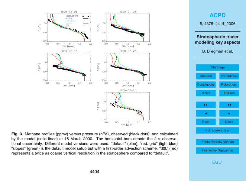
Figure 3 shows a comparison with observations for the model versions “de-fault”,“red. grid”, “slopes”, and “30L”. In December the model results are close to theobservations. However, the model overestimates CH4 later in the winter and the over-estimation increases in time. Note that the “slopes” results are similar to those pre-sented in van den Broek et al. (2003) and considerably overestimates the observed20

CH4 profiles. Another feature is the significant improvement when applying less dif-fusive second-order moments advection. However, the model still overestimates thetracer concentrations. The results from the “red. grid” run are similar to the “slopes”run, but are performed with the second-order moments advection scheme, and reflectsthe effect of the reduced polar grid. This quite dramatic effect is also visible in Fig. 2.25

This result is quite remarkable, since the reduced grid extends to 70◦ N only, while theballoon profiles were located more southwards.

The improvement when removing the reduced polar grid gives an important mes-4387





ACPD6, 4375–4414, 2006


B. Bregman et al.

Title Page



Tables Figures

J I

J I

Back Close

Full Screen / Esc



EGU

sage to those who apply some kind of grid or mass flux or wind vector merging in thepolar region. Another important effect is that a reduction of the polar grid obscuresevaluation of grid resolution. To demonstrate this we applied the diffusive first-orderslopes advection, as was done in van den Broek et al. (2003) but now with model gridzooming up to the pole (run “1×1”). Figure 4 shows that the results improved signifi-5

cantly and are comparable or occasionally even slightly better then the results from thedefault run with second-order moments advection. This is in contrast with the previ-ous evaluation in van den Broek et al. (2003) where grid zooming did not improve theresults and clearly demonstrate the danger of polar grid reduction.

The significant improvement in tracer distribution when increasing the horizontal res-10

olution from 3◦×2◦ to 1◦×1◦ illustrates that model grid resolution is a key issue for thediffusivity of advection. The “1×1” run used the relatively diffusive first-order slopesadvection scheme, while the “default” run used much less diffusive second-order mo-ments advection.

The numerical diffusion depends on the amount of tracer information for a given grid15

cell volume. Figure 6 shows the tracer information for a 3◦×2◦ grid cell in the case of the“default” run (left panel), the “slopes” run (middle panel) and the “1×1” run (right panel).The “default” run contains 10 parameters that determine the tracer level: the first-orderslopes (3), the second-order moments (6), and the tracer mass (1). In contrast, the“slopes” run only contains 4 variables with tracer information: the first-order slopes (3)20

and the tracer mass (1). On the other hand, the zoom region contains 6 more grid cellswith each 4 tracer parameters, resulting in a total of 24. The “slopes” run contains theleast amount of tracer information and clearly yields the worst results. However, theamount of tracer information in the “1×1” run is twice more than that of the “default”configuration for a 3◦×2◦ grid cell, but shows no improvement in the tracer distribution.25

This may indicate a resolution threshold, which support the findings by Searle et al.(1998). However, this study demonstrates that such a threshold, if present, depends onthe way tracer advection is performed. A diffusive advection scheme clearly overrulesthe advantage of resolution increase, at least up to 1◦×1◦. It will also depend on the

4388





ACPD6, 4375–4414, 2006


B. Bregman et al.

Title Page



Tables Figures

J I

J I

Back Close

Full Screen / Esc



EGU

chemical lifetime of the tracer in question and for a species such as ClO the impact ofresolution increase may be substantial (Marchand et al., 2003; Tan et al., 1998).

Next a sensitivity test of vertical resolution was performed. By comparing “default”with “30L” Fig. 3 shows that the effect of doubling the vertical resolution is restricted tothe upper stratosphere (i.e., above the 10 hPa pressure level) where both profiles start5

to deviate. Due to the limited altitude range of the balloon, no detailed comparisoncould be performed in the upper stratosphere. Nevertheless, these results indicatethat for the current model configuration and experimental setup, vertical resolution doeshave a significant impact on the tracer distribution, but only in the upper stratosphere.

Finally, we examined the effect of using more wind variability as given by the assim-10

ilated wind fields. Figure 5 shows the calculated CH4 profiles from the “default” run,i.e., with instantaneous 6-hourly wind fields, similar as in Fig. 3 and 6. By interpolatingthe winds between two subsequent time intervals we account for the wind variabilitywithin the model integration time interval. The agreement with observations improves,especially on 15 March 2000. Applying 3-hourly interpolated winds the results are in15

excellent agreement with the observations.These results demonstrate the importance to avoid constant winds within the me-

teorological time interval and in particular the importance of the update frequency ofthe DAS winds, which was also shown for mid-latitude tracer profiles in Berthet et al.(2006). Apparently, more real variability is introduced when applying 3-hourly instead20

of 6-hourly winds, rather than more “noise”.

4.3 Comparison with satellite observations: tracer gradient across the vortex edge

Next, we focus on the tracer gradient through the vortex edge. A comparison is per-formed with 15 profiles observed by the HALOE instrument on board the UARS satel-lite. See van den Broek et al. (2003) for a more detailed description of these observa-25

tions. These profiles were part of the HALOE sweeps close to the edge of the polarvortex, covering both mid-latitudinal extra- and polar vortex air, and are thus very suit-able to focus on the vortex edge. For such a comparison an equivalent, instead of the

4389





ACPD6, 4375–4414, 2006


B. Bregman et al.

Title Page



Tables Figures

J I

J I

Back Close

Full Screen / Esc



EGU

regular Cartesian, latitude coordinate is more useful. Three different potential temper-ature levels have been selected, one close to the polar vortex bottom (425 K), one inthe lower stratosphere (500 K) and one in the middle stratosphere (600 K).

Figures 7, 8 and 9 show the results of this comparison for the “default”, “red. grid”,“1×1” runs, “6-hourly-interp” and “3-hourly-interp” experiments. The comparisons are5

somewhat obscured by the relatively large scatter in the observations, the limited cov-erage in the polar vortex and the modeled variability (denoted by the vertical bar as1σ). The scatter in the observations is most probably due to the differences in thesampling volume of the observations and the ECWMF potential temperature and po-tential vorticity grid cell volumes. Nevertheless, the latitudinal coverage is sufficient10

and the tracer gradient across the vortex edge is clearly discernible. As expected, thegradient becomes more pronounced with increasing potential temperature level, bothin the observations and in the model results. The default run agrees quite reasonable,while significant underestimation is found for the “red. grid” run, in line with the findingsin Fig. 3. The tracer gradient at the vortex edge is manifested most clearly in the “1×1”15

run, although the overall gradient is similar to the default run.It is interesting that the modeled variability is significantly reduced in the zoom region,

especially in active mixing regions: close to the vortex bottom and at the vortex edge.This reflects the increased tracer information in the zoom region, despite the morediffusive advection scheme (see Fig. 6).20

Figure 7 indicates that the impact of the reduced grid exceeds the polar region. Thesouthern border of the reduced grid in the Arctic is 70◦ N, but the differences with thedefault run extends to 60◦ N equivalent latitude. It is remarkable that the impact isfound even further south in instantaneous fields. As was demonstrated in Fig. 8 thedifferences with the zoom region are small with differences up to about 10% and arise25

at locations where vortex filaments are present.As can be seen in Fig. 9 the calculated gradients became stronger when introducing

time interpolation and in particular by increasing the meteorological update frequency,in line with the model results described earlier. The differences with the results from the

4390





ACPD6, 4375–4414, 2006


B. Bregman et al.

Title Page



Tables Figures

J I

J I

Back Close

Full Screen / Esc



EGU

default run increase with increasing potential temperature level. At 600 K the model un-derestimates the observations at 50–60◦ N outside the polar vortex, which is apparentin the results from all model experiments.

Note that even in the best model performance the calculated gradient is slightly un-derestimated, indicating remaining diffusivity and/or the lack of chemistry. Although the5

effect of chemistry has been tested to have a negligible impact on methane at levelsbelow 10 hPa in a similar model experiment (van Aalst et al., 2004), caution must betaken by treating methane as a passive tracer. Especially close to more chemicallyactive regions of the atmosphere, i.e., the upper stratosphere outside the polar vortex.Indicative for this influence could be the slight underestimation by the model in Figs. 810

and 9 at the highest potential temperature level (600 K), which is not present at lowerpotential temperature levels.

4.4 Age of air experiment

In this experiment we focus on the large-scale meridional circulation in the stratosphereby calculating the mean age of air, as described in the section experimental setup.15

Here we examine if the earlier found disagreements in calculated and observed meanage of air (Meijer et al., 2004) can be improved by applying 3-hourly DAS winds andtime interpolation. We also omitted the reduced polar grid. For the evaluation of themodeled mean age of air we use a compilation of CO2 and SF6 observed on board theER-2 between 1991–1998 (Andrews et al., 2001), as in Meijer et al. (2004).20

Figure 10 shows the calculated zonally average mean age of air for three differentruns using 6-hourly instantaneous (top panel), 6-hourly interpolated (middle panel) and3-hourly interpolated winds (bottom panel). The mean age of air is significantly olderwhen using 3-hourly instead of 6-hourly interpolated winds. The effect of interpolationis less significant, although the air becomes 0.5 year older in the upper stratosphere25

when applying time interpolating in the 6-hourly winds.Figure 11 shows the calculated zonally average mean age of air for the same three

runs, but now at approximately 20 km altitude, compared to observations. The obser-4391





ACPD6, 4375–4414, 2006


B. Bregman et al.

Title Page



Tables Figures

J I

J I

Back Close

Full Screen / Esc



EGU

vations represent mean age of air derived from airborne in-situ CO2 measurementson board the ER-2 aircraft in the lower stratosphere (Andrews et al., 2001). The mea-surements are a compilation of all observations between 1991 and 1998. In line withFig. 10 the use of 3-hourly interpolated winds gives the oldest mean age of air. Notethat the meridional gradient is significantly steeper than using 6-hourly winds, indica-5

tive of reduced dispersion. Nevertheless the calculated mean age still remains aboutone year too young in the extra-tropical lower stratosphere. Applying time interpolationin the 6-hourly winds only yields a small improvement. As shown in Fig. 10 the effectof time interpolation is discernible mainly in the middle and upper stratosphere.

The mean age of air from the 6-hourly instantaneous winds is similar to that calcu-10

lated by Meijer et al. (2004), although they applied a reduced polar grid. This indicatesthat, in contrast to the findings in the polar study, the reduced polar grid does not affectthe stratospheric large-scale tracer transport.

4.5 Back-trajectory experiments

Next we focus on the tropical lower stratosphere, since it is a key region for the large-15

scale meridional circulation. With back-trajectory calculations we calculate the disper-sion of air parcels over 50 days. This time scale is much shorter than the mean age ofair, but the dispersion intensity is a useful measure of the noise in DAS winds and thusindirectly relates to the mean age of air (Schoeberl et al., 2002; Scheele et al., 2005).In these calculations we only used interpolated winds. So far we have examined the20

effect of increasing the update frequency with 4DVAR OD data only. It is interesting toinvestigate the effect using 3DVAR ERA40 data. We therefore examined three differentDAS winds: (1) the default OD 6-hourly winds (red line), similar to the results in Fig. 2in Scheele et al. (2005). The second and third data set is derived from the 3DVARERA40 6-hourly and 3-hourly winds, respectively. Figure 12 shows the end points of25

the air parcels after 50 days. There is considerable scatter, similar to the results fromSchoeberl et al. (2002). As expected, the 6-hourly winds from OD are less dispersivethan those from ERA40, as already discussed by Scheele et al. (2005). However, the

4392





ACPD6, 4375–4414, 2006


B. Bregman et al.

Title Page



Tables Figures

J I

J I

Back Close

Full Screen / Esc



EGU

3-hourly winds from ERA40 show much less vertical dispersion, even compared to thegenerally less noisy OD winds. Interestingly, the horizontal dispersion is not reducedin the 3-hourly winds.

Figure 13 shows the fraction of air parcels leaving the 10◦ S–10◦ N latitude bandbefore crossing the tropopause as a measure of dispersion versus the integration time5

(50 days). In line with Fig. 12, the 3DVAR winds (ERA40 6-hourly) show a significantlarge fraction than the 4DVAR winds (OD 6-hourly). This result is similar as in Scheeleet al. (2005). Adding the 3-hourly ERA40 data results in a strong decrease of thefraction. It is even smaller than that calculated with the 6-hourly OD using 4DVARassimilation.10

5 Conclusions

In this study we used a CTM (TM5) to investigate the impact of a variety of differentmodel configurations and different representations of the assimilated meteorology onstratospheric tracer transport. In particular we examined the impact of model grid reso-lution, including the reduction of the polar grid, the diffusivity of the advection scheme,15

and the update frequency and variability in DAS winds. As a diagnose we used CH4transport in the Arctic polar vortex and the mean age of air. We further applied atrajectory model to investigate air parcel dispersion in the tropical lower stratosphere.

This study shows that the commonly applied artificial reduction of the polar grid ofwind field averaging does have a significant impact on the tracer distribution. The20

impact well exceeds the area of the reduced grid and these results contain an importantmessage for other studies on polar tracer transport with global models.

The sensitivity experiments show that doubling the vertical resolution substantiallyaffects the tracer distribution in the upper stratosphere, i.e., above 10 hPa, but not belowthis pressure level. The model results in the upper stratosphere can unfortunately not25

be evaluated due to a lack of observations.On the course of a winter increasing the horizontal resolution to 1◦×1◦ improves the

4393





ACPD6, 4375–4414, 2006


B. Bregman et al.

Title Page



Tables Figures

J I

J I

Back Close

Full Screen / Esc



EGU

CH4 distribution in the polar vortex considerably when using first-order (slopes) advec-tion. This is to be expected, since a higher grid resolution represents the vortex edgemore realistically. Note that this is only valid without a reduced polar grid. These resultsare an update of a previous model study where an increase in horizontal grid resolu-tion did not improve the tracer distributions using the same experimental setup. This5

contrasting result clearly demonstrates the danger of using a reduced polar grid whenevaluating model grid resolution. By using adjustable advection time steps, proper highresolution global modeling is feasible in the polar regions.

The impact on stratospheric CH4 distribution in the polar region by applying morewind variability in the CTM integrations is significant. Using 6-hourly time interpolated10

instead of instantaneous winds resulted in reduced cross vortex edge mixing and closeragreement with the observed CH4 profiles inside the vortex. Reducing the time intervalto 3 h improves the model results even further and yielded excellent agreement withthe observed CH4 profiles inside the Arctic vortex.

The stratospheric meridional circulation is examined by diagnosing the mean resi-15

dence time of air in the stratosphere (mean age of air). The mean age of air becomessignificantly older in the extra-tropical stratosphere when applying 3-hourly instead of6-hourly interpolated winds. This indicates that introducing more variability in the windfields reduces the dispersion. The use of time interpolation is particularly noticeable inthe middle and upper stratosphere where the mean age of air becomes 0.5 year older.20

The tropical mean age of air shows excellent agreement with observations, althoughthe extra-tropical lower stratospheric mean age remains too young with about one year.

According to the back-trajectory calculations, the use of 3-hourly winds leads to lessvertical dispersion, even with winds produced by the more noisy ERA40 re-analyseswinds. It is important to note that the use of 3-hourly winds does not introduce more25

noise, but more real variability in the wind fields. It remains to be determined what isthe most suitable update frequency for stratospheric tracer transport. Such a questionis directly related to the representation of the winds from the GCM that provides thewinds to the data assimilation system. Waugh et al. (1997) discussed different time

4394





ACPD6, 4375–4414, 2006


B. Bregman et al.

Title Page



Tables Figures

J I

J I

Back Close

Full Screen / Esc



EGU

intervals and averaging, however, not for time frequencies of 3 or even less hours.Investigating this problem is however not trivial and is subject of further study.

For models using vertical hybrid sigma-pressure coordinates recent new insights inthe use of DAS winds in CTMs has improved the stratospheric tracer representationconsiderably, both in the polar region as on the large scale. It is recommended not to5

use a reduction of the polar grid (either through grid cell merging or by wind averag-ing). We also recommend to apply time interpolation instead of using instantaneouswinds. In line with the findings from Legras et al. (2005) it is also recommended toapply 3-hourly instead of the commonly used 6-hourly update interval. These results incombination with improvements in data assimilation procedures give new perspectives10

for long-term tracer integrations.

Acknowledgements. Part of this work is funded by the European Commission, through theproject TOwards the Prediction of stratospheric OZone (TOPOZ) III, under contract no. EVK2-CT-2001-00102, the project Stratospheric-Climate Links with Emphasis on the Upper Tropo-sphere and Lower Stratosphere (SCOUT), and the National (Netherlands) User Support Pro-15

gramme (GO)2. We thank M. Krol and A. Segers for computational support and useful discus-sions.

References

Andrews, A., Boering, K., Daube, B., Wofsy, S., Loewenstein, M., Jost, H., Podolske, J., Web-ster, C., Herman, R., Scott, D., Flesh, G., Moyer, E., Elkins, J., Dutton, G., Hurst, D., Moore,20

F., Ray, E., Romanshkin, P., and Strahan, S.: Mean ages of stratospheric air derived fromin situ observations of CO2, CH4, and N2O, J. Geophys. Res., 106, 32 295–32 314, 2001.4391, 4392, 4412

Berthet, G., Huret, N., Lefevre, F., Moreau, G., Robert, C., Chartier, M., Pomathiod, L., Pirre,M., and Catoire, V.: On the ability of chemical transport models to simulate the vertical25

structure of the N2O, NO2 and HNO3 species in the mid-latitude stratosphere, Atmos. Chem.Phys., 6, 1599–1609, 2006. 4381, 4386, 4389

4395





ACPD6, 4375–4414, 2006


B. Bregman et al.

Title Page



Tables Figures

J I

J I

Back Close

Full Screen / Esc



EGU

Bregman, A., Krol, M., Teyssedre, H., Norton, W., Chipperfield, M., Pitari, G., Sundet, J., andLelieveld, J.: Chemistry-transport model comparison with ozone observations in the midlati-tude lowermost stratosphere, J. Geophys. Res., 106, 17 479–17 496, 2001. 4382

Bregman, A., Wang, P.-H., and Lelieveld, J.: Chemical ozone loss in the tropopause region onsubvisible ice clouds, calculated with a chemistry-transport model, J. Geophys. Res., 107,5

doi:10.1029/2001JD000761, 2002. 4382Bregman, B., Segers, A., Krol, M., Meijer, E., and van Velthoven, P.: On the use of mass-

conserving wind fields in chemistry-transport models, Atmos. Chem. Phys., 3, 447–457,2003. 4380, 4383

Chipperfield, M.: New version of the TOMCAT/SLIMCAT off-line chemical transport model:10

Intercomparison of stratospheric tracer experiments, Q. J. R. Meteorol. Soc., in press, 2006.4379, 4380

Dentener, F., Feichter, J., and Jeuken, A.: Simulation of the transport of Rn222 using on-lineand off-line global models at different horizontal resolutions: A detailed comparison withmeasurements, Tellus, 51, 573–602, 1999. 438215

Douglass, A., Schoeberl, M. R., Rood, R. B., and Pawson, S.: Evaluation of transport in thelower tropical stratosphere in a global chemistry and transport model, J. Geophys. Res., 108,4259, doi:10.1029/2002JD002696, 2003. 4378

Garcelon, S., Gardiner, T., Hansford, G., Harris, N., Howieson, I., Jones, R., McIntyre, J.,Pyle, J., Robinson, J., Swann, N., and Woods, P.: Investigation of CH4 and CFC-11 vertical20

profiels in the Arctic vortex during the SOLVE/THESEO 2000 campaign, in: Proceedings ofthe general Assembly, Nice, European Geophyisical Society, 2002. 4387

Hadjinicolaou, P., Pyle, J. A, and Harris, N. R. P.: The recent turnaround in stratospheric ozoneover northern middle latitudes: A dynamical modeling perspective, Geophys. Res. Lett., 32,L12821, doi:10.1029/2005GL022476, 2005. 437925

Hall, T. and Plumb, R.: Age as a diagnostic of stratospheric transport, J. Geophys. Res., 99,1059–1070, 1994. 4384

Hall, T., Waugh, D., Boering, K., and Plumb, R.: Evaluation of transport in stratospheric models,J. Geophys. Res., 104, 18 815–18 839, 1999. 4384

Heimann, M.: The Global Atmospheric Tracer Model TM2, Tech. Rep. 10, DRKZ-Hamburg,30

1995. 4382Heimann, M. and Keeling, C.: A three-dimensional model of atmospheric CO2 transport based

on observed winds: 2: Model description and simulated tracer experiments, Geophys. Mon.,

4396





ACPD6, 4375–4414, 2006


B. Bregman et al.

Title Page



Tables Figures

J I

J I

Back Close

Full Screen / Esc



EGU

55, 237–275, 1989. 4382Houweling, S., Dentener, F., and Lelieveld, J.: The impact of non-methane hydrocarbon com-

pounds on tropospheric photochemistry, J. Geophys. Res., 103, 10 673–10 696, 1998. 4382Jockel, P., von Kuhlmann, R., Lawrence, M., Steil, B., Brenninkmeijer, C., Crutzen, P., Rasch,

P., and Eaton, B.: On a fundamental problem in implementing flux-form advection schemes5

for tracer transport in 3-dimensional general circulation and chemistry transport models, Q.J. R. Meteorol. Soc., 127, 1035–1052, 2001. 4380

Krol, M., Houweling, S., Bregman, B., van den Broek, M., Segers, A., van Velthoven, P., Peters,W., Dentener, F., and Bergamaschi, P.: TM5, a global two-way nested chemistry transportzoom model: algorithm and applications, Atmos. Chem. Phys., 5, 417–432, 2005. 4378,10

4383Laat, A., Landgraf, J., Aben, I., Hasekamp, O., and Bregman, B.: Assimilated winds for global

modelling: evaluation with space- and balloon-borne ozone observations, J. Geophys. Res.,in press, 2006. 4379

Legras, B., Pisso, I., Berthet, G., and Lefevre, F.: Variability of the Lagrangian turbulent diffusion15

in the lower stratosphere, Atmos. Chem. Phys., 5, 1605–1622, 2005. 4381, 4395Mahowald, N. M., Plumb, R. A., Rasch, P. J., del Corral, J., Sassi, F., and Heres, W.: Strato-

spheric transport in a three-dimensional isentropic coordinate model, J. Geophys. Res.,107(D15), 4254, doi:10.1029/2001JD001313, 2002. 4380

Manney, G., Allen, D., Kruger, K., Naujokat, B., Santee, M., Sabutis, J., Pawson, S., Swinbank,20

R., Randall, C., Simmons, A. J., and Long, G.: Diagnosic comparison of meteorologicalanalyses during the 2002 Antarctic winter, J. Atmos. Sci., 133, 1261–1278, 2005. 4379

Manson, A., Meek, C., Koshyk, J., Franke, S., Fritts, D., Riggin, D., Hall, C., Hocking, W.,MacDougall, J., Igarashi, K., and Vincent, R.: Gravity wave activity and dynamical effectsin the middle atmosphere (60–90 km): observations from an MF/MLT radar network, and25

results from the Canadian Middle Atmosphere Model (CMAM), J. Atmos. Solar-Terr. Phys.,64, 65–90, 2002. 4381

Marchand, M., Godin, S., Hauchecorne, A., Lefevre, F., and Chipperfield, M.: Influ-ence of polar ozone loss on northern midlatitude regions estimated by a high-resolutionchemistry transport model during winter 1999/2000, J. Geophys. Res., 108, 8326,30

doi:10.1029/2001JD000906, 2003. 4377, 4389Meijer, E. W., Bregman, B., Segers, A., and van Velthoven, P. F. J.: The influence of data as-

similation on the age of air calculated with a global chemistry-transport model using ECMWF

4397





ACPD6, 4375–4414, 2006


B. Bregman et al.

Title Page



Tables Figures

J I

J I

Back Close

Full Screen / Esc



EGU

winds, Geophys. Res. Lett., 31, L23114, doi:10.1029/2004GL021158, 2004. 4378, 4379,4380, 4391, 4392

Peters, W., Krol, M. C., Dentener, F. J., and Lelieveld, J.: Identification of an El Nino-SouthernOscillation signal in a multiyear global simulation of tropospheric ozone, J. Geophys. Res.,106, 10 389–10 402, 2001. 43825

Polavarapu, S., Ren, S., Rochon, Y., Sankey, D., Ek, N., Koshyk, J., and Tarasick, D.: Dataassimilation with the Canadian Middle Atmosphere Model, Appl. Opt., 43, 77–100, 2005.4381

Prather, M.: Numerical advection by conservation of second-order moments, J. Geophys. Res.,91, 6671–6681, 1986. 4383, 438510

Randel, W., Fleming, E., Geller, M., Gelman, M., Hamilton, K., Karoly, D., Ortland, D., Pawson,S., Swinbank, R., Udelhofen, P., Wu, F., Baldwin, M., Chanin, M.-L., Keckhut, P., Simmons,A., and Wu, D.: The SPARC intercomparison of Middle Atmosphere Climatologies, Tech.Rep. 20, SPARC newsletter, 2003. 4379

Rotman, D., Atherton, C., Bergmann, D., Cameron-Smith, P., Chuang, C., Connell, P., Dignon,15

J., Franz, A., Grant, K., Kinnison, D., Molenkamp, C., Proctor, D., and Tannahill, J.: IMPACT,the LLNL 3-D global atmospheric chemical transport model for the combined troposphereand stratosphere: Model description and analysis of ozone and other trace gases, J. Geo-phys. Res., 109, D04303, doi:10.1029/2002JD003155, 2004. 4380

Russel, G. and Lerner, J.: A new finite-differencing scheme for the tracer transport equation, J.20

Appl. Meteorol., 20, 1483–1498, 1981. 4383, 4385Russel-III, J., Gordley, L., Park, J., Drayson, S., Hesketh, D., Cicerone, R., Tuck, A., Frederick,

J., Harries, J., and Crutzen, P.: The Halogen Occultation Experiment, J. Geophys. Res., 98,10 777–10 797, 1993. 4387

Scheele, R., Siegmund, P., and van Velthoven, P.: Stratospheric age of air computed with25

trajectories based on various 3-D-Var and 4-D-Var data sets, Atmos. Chem. Phys., 5, 1–7,2005. 4378, 4379, 4380, 4384, 4385, 4392, 4393

Schoeberl, M., Douglass, A., Zhu, Z., and Pawson, S.: A comparison of the lower stratosphericage-spectra, derived from a General Circulation Model and two data assimilation systems.,J. Geophys. Res., 108, 4113, doi:10.1029/2002JD002652, 2002. 4378, 4385, 439230

Searle, K., Chipperfield, M., Bekkie, S., and Pyle, J.: The impact of spatial averaging on calcu-lated polar ozone loss, 1, Model experiments, J. Geophys. Res., 103, 25 397–25 408, 1998.4377, 4388

4398





ACPD6, 4375–4414, 2006


B. Bregman et al.

Title Page



Tables Figures

J I

J I

Back Close

Full Screen / Esc



EGU

Segers, A., van Velthoven, P., Bregman, B., and Krol, M.: On the computation of mass fluxes forEulerian transport models from spectral meteorological fields, in: Proceedings of the 2002International Conference on Computational Science, Lecture Notes in Computer Science(LNCS), Springer Verlag, 2002. 4380, 4382

Shepherd, T., Koshyk, J., and Ngan, K.: On the nature of large-scale mixing in the stratosphere5

and mesosphere, J. Geophys. Res., 105, 12 433–12 446, 2000. 4381Simmons, A., Hortal, M., Kelly, G., McNally, A., Untch, A., and Uppala, S.: ECMWF analyses

and forecasts of stratospheric winter polar vortex breakup: September 2002 in the SouthernHemisphere and related events, J. Atmos. Sci., 62, 668–689, 2005. 4379

Tan, D., Haynes, P. H., MacKenzie, A. R., and Pyle, J. A.: Effects of fluid-dynamical stirring10

and mixing on the deactivation of stratospheric chlorine, J. Geophys. Res., 103, 1585–1606,1998. 4389

Toon, G., Blavier, J.-F., Sen, B., Margitan, J., Webster, C., May, R., Fahey, D., Gao, R., Negro,L. D., Proffit, M., Elkins, J., Romashkin, P., Hurst, D., Oltmans, S., Atlas, E., Schauffler, S.,Flocke, F., Bui, T., Stimpfle, R., Boone, G., Voss, P., and Cohen, R.: Comparison of MkIV15

balloon and ER-2 aircraft measurements of atmospheric trace gases, J. Geophys. Res., 104,26 779–26 790, 1999. 4387

van Aalst, M., van den Broek, M., Bregman, A., Bruhl, C., Steil, B., Toon, G., Garcelon, S.,Hansford, G., Jones, R., Gardiner, T., Roelofs, G., Lelieveld, J., and Crutzen, P.: Tracertransport in the 1999/2000 Arctic polar vortex comparison of nudged GCM runs with obser-20

vations, Atmos. Chem. Phys., 4, 81–93, 2004. 4391Van den Broek, M., Bregman, A., and Lelieveld, J.: Model study of stratospheric chlorine and

ozone loss during the 1996/1997 winter, J. Geophys. Res., 105, 28 961–28 977, 2000. 4382van den Broek, M., van Aalst, M., Bregman, A., Krol, M., Lelieveld, J., Toon, G., Garcelon,

S., Hansford, G., Jones, R., and Gardiner, T.: The impact of model grid zooming on tracer25

transport in the 1999/2000 Arctic polar vortex, Atmos. Chem. Phys., 3, 1833–1847, 2003.4377, 4382, 4383, 4384, 4385, 4386, 4387, 4388, 4389

van Noije, T. P. C., Eskes, H. J., van Weele, M., and van Velthoven, P. F. J.: Implications ofthe enhanced Brewer-Dobson circulation in European Centre for Medium-Range WeatherForecasts reanalysis ERA-40 for the stratosphere-troposphere exchange of ozone in global30

chemistry transport models, J. Geophys. Res., 109, D19308, doi:10.1029/2004JD004586,2004. 4379

Waugh, D. W., Hall, T. M., Randel, W. J., Rasch, P. J., Boville, B. A., Boering, K. A., Wofsy, S. C.,

4399





ACPD6, 4375–4414, 2006


B. Bregman et al.

Title Page



Tables Figures

J I

J I

Back Close

Full Screen / Esc



EGU

Daube, B. C., Elkins, J. W., Fahey, D. W., Dutton, G. S., and Volk, C. M.: Three-dimensionalsimulations of long-lived tracers using winds from MACCM2, J. Geophys. Res., 102(D17),21 493–21 514, 1997. 4394

Wild, O., Sundet, J. K., Prather, M. J., Isaksen, I. S. A., Akimoto, H., Browell, E. V., and Oltmans,S. J.: Chemical transport model ozone simulations for spring 2001 over the western Pacific:5

Comparisons with TRACE-P lidar, ozonesondes and Total Ozone Mapping Spectrometercolumns, J. Geophys. Res., 108(D21), 8826, doi:10.1029/2002JD003283, 2003. 4381

WMO: Scientific Assessment of Ozone Depletion, Tech. Rep. 47, WMO, 2002. 4377

4400





ACPD6, 4375–4414, 2006


B. Bregman et al.

Title Page



Tables Figures

J I

J I

Back Close

Full Screen / Esc



EGU

Table 1. A summary of the model experiments. See text for more details for each experiment.

Experiment advection resolution vertical layers winds

“default” or “3×2” 2nd moments 3◦×2◦ 45 6-hourly instantaneous“red. grid” 2nd moments 3◦×2◦ 45 6-hourly instantaneous“slopes” 1st moments 3◦×2◦ 45 6-hourly instantaneous“30L” 2nd moments 3◦×2◦ 30 6-hourly instantaneous“1×1” 1st moments 1◦×1◦ 45 6-hourly instantaneous“6-hrly interp.” 2nd moments 3◦×2◦ 45 6-hourly time interpolated“3-hrly interp.” 2nd moments 3◦×2◦ 45 3-hourly time interpolated

4401





ACPD6, 4375–4414, 2006


B. Bregman et al.

Title Page



Tables Figures

J I

J I

Back Close

Full Screen / Esc



EGU

12 Bram Bregman: STRATOSPHERIC TRACER MODELING KEY ASPECTS

Fig. 1. A schematic view of the trajectory experimental setup. Seetext for more details.

Atmos. Chem. Phys., 0000, 0001–24, 2006 www.atmos-chem-phys.org/0000/0001/

Fig. 1. A schematic view of the trajectory experimental setup. See text for more details.

4402





ACPD6, 4375–4414, 2006


B. Bregman et al.

Title Page



Tables Figures

J I

J I

Back Close

Full Screen / Esc



EGU

Bram Bregman: STRATOSPHERIC TRACER MODELING KEY ASPECTS 13

Fig. 2. Horizontal cross sections of methane mixing ratios (ppmv) at35 hPa, 15 March 2000, 0 GMT for the ’default’, ’reduced grid’ and’1x1’ runs with 6-hourly instantaneous (constant) winds, and withthe default configuration busing 6-hourly and 3-hourly interpolatedwinds.

www.atmos-chem-phys.org/0000/0001/ Atmos. Chem. Phys., 0000, 0001–24, 2006

Fig. 2. Horizontal cross sections of methane mixing ratios (ppmv) at 35 hPa, 15 March 2000,00:00 GMT for the “default”, “reduced grid” and “1×1” runs with 6-hourly instantaneous (con-stant) winds, and with the default configuration busing 6-hourly and 3-hourly interpolated winds.

4403





ACPD6, 4375–4414, 2006


B. Bregman et al.

Title Page



Tables Figures

J I

J I

Back Close

Full Screen / Esc



EGU


Fig. 3. Methane profiles (ppmv) versus pressure (hPa), observed(black dots), and calculated by the model (solid lines) at March 15,2000. The horizontal bars denote the 2-σ observational uncertainty.Different model versions were used: ’default’ (blue), ’red. grid’(light blue) ’slopes’ (green) is the default model setup but witha first-order advection scheme. ’30L’ (red) represents a twice ascoarse vertical resolution in the stratosphere compared to ’default’.


Fig. 3. Methane profiles (ppmv) versus pressure (hPa), observed (black dots), and calculatedby the model (solid lines) at 15 March 2000. The horizontal bars denote the 2-σ observa-tional uncertainty. Different model versions were used: “default” (blue), “red. grid” (light blue)“slopes” (green) is the default model setup but with a first-order advection scheme. “30L” (red)represents a twice as coarse vertical resolution in the stratosphere compared to “default”.

4404





ACPD6, 4375–4414, 2006


B. Bregman et al.

Title Page



Tables Figures

J I

J I

Back Close

Full Screen / Esc



EGU


Fig. 4. As figure 3, but with the results from the default (blue) and’1x1’ (red) runs. Day 2000-02-27 has been omitted.


Fig. 4. As Fig. 3, but with the results from the default (blue) and “1×1” (red) runs. Day 2000-02-27 has been omitted.

4405





ACPD6, 4375–4414, 2006


B. Bregman et al.

Title Page



Tables Figures

J I

J I

Back Close

Full Screen / Esc



EGU


Fig. 5. As figure 3, but with the results from the default run (blue),using 6-hourly interpolated (green) and 3-hourly interpolated (red)winds. Day 2000-02-27 has been omitted.


Fig. 5. As Fig. 3, but with the results from the default run (blue), using 6-hourly interpolated(green) and 3-hourly interpolated (red) winds. Day 2000-02-27 has been omitted.

4406





ACPD6, 4375–4414, 2006


B. Bregman et al.

Title Page



Tables Figures

J I

J I

Back Close

Full Screen / Esc



EGU


mrxm, rym, rzmrxxm, rxym, rxzmryym, ryzm, rzzm

mrxm, rym, rzm

mrxmrymrzm

mrxmrymrzm

mrxmrymrzmm

rxmrymrzm

mrxmrymrzm

mrxmrymrzm

'default' 30x20 'slopes' 30x20 'slopes' 10x10

Fig. 6. A schematic view of the tracer information per grid cell of3◦x2◦, when applying second-moments (left) and first-order advec-tion without grid zooming (middle) and with grid zooming (right).


Fig. 6. A schematic view of the tracer information per grid cell of 3◦×2◦, when applying second-moments (left) and first-order advection without grid zooming (middle) and with grid zooming(right).

4407





ACPD6, 4375–4414, 2006


B. Bregman et al.

Title Page



Tables Figures

J I

J I

Back Close

Full Screen / Esc



EGU


Fig. 7. Observed methane profiles volume mixing ratios in ppmv(black dots) at March 15, 2000, 0 GMT, and calculated by the modelwith the default model setup, with (red dots) and without (blue dots)the reduced polar grid. The comparison is performed at equiva-lent latitude (degrees) and three different isentropic levels (425 K,500 K, and 600 K). The vertical bars represent 2σ variability of themodel results.


Fig. 7. Observed methane profiles volume mixing ratios in ppmv (black dots) at 15 March2000, 00:00 GMT, and calculated by the model with the default model setup, with (red dots)and without (blue dots) the reduced polar grid. The comparison is performed at equivalentlatitude (degrees) and three different isentropic levels (425 K, 500 K, and 600 K). The verticalbars represent 2σ variability of the model results.

4408





ACPD6, 4375–4414, 2006


B. Bregman et al.

Title Page



Tables Figures

J I

J I

Back Close

Full Screen / Esc



EGU


Fig. 8. Similar as figure 7, but with the results from the default (reddots) and ’1x1’(blue dots) runs.


Fig. 8. Similar as Fig. 7, but with the results from the default (red dots) and “1×1” (blue dots)runs.

4409





ACPD6, 4375–4414, 2006


B. Bregman et al.

Title Page



Tables Figures

J I

J I

Back Close

Full Screen / Esc



EGU


Fig. 9. Similar as figure 7, but with the results from the runs withthe 3-hourly (blue dots) and 6-hourly (red dots) interpolated winds.


Fig. 9. Similar as Fig. 7, but with the results from the runs with the 3-hourly (blue dots) and6-hourly (red dots) interpolated winds.

4410





ACPD6, 4375–4414, 2006


B. Bregman et al.

Title Page



Tables Figures

J I

J I

Back Close

Full Screen / Esc



EGU


Fig. 10. Calculated latitudinal cross section of zonally averagemean age of air (years) for three different experiments with second-order moments advection and without a reduced polar grid: using6-hourly instantaneous (top panel), 6-hourly interpolated (middlepanel) and the 3-hourly interpolated winds (bottom panel) respec-tively.


Fig. 10. Calculated latitudinal cross section of zonally average mean age of air (years) for threedifferent experiments with second-order moments advection and without a reduced polar grid:using 6-hourly instantaneous (top panel), 6-hourly interpolated (middle panel) and the 3-hourlyinterpolated winds (bottom panel) respectively.

4411





ACPD6, 4375–4414, 2006


B. Bregman et al.

Title Page



Tables Figures

J I

J I

Back Close

Full Screen / Esc



EGU


Fig. 11. Observed and calculated mean age of air for the same ex-periments as in figure 10. The observations (black dots) are derivedfrom multi-year CO2 observations from the ER-2 at approximately20 km altitude (Andrews et al., 2001). The error bars represent 2-σstandard deviation.


Fig. 11. Observed and calculated mean age of air for the same experiments as in Fig. 10.The observations (black dots) are derived from multi-year CO2 observations from the ER-2 atapproximately 20 km altitude (Andrews et al., 2001). The error bars represent 2-σ standarddeviation.

4412





ACPD6, 4375–4414, 2006


B. Bregman et al.

Title Page



Tables Figures

J I

J I

Back Close

Full Screen / Esc



EGU


Fig. 12. The end locations of the air parcels after 50 daysback-trajectory calculations for OD data with 6-hourly interpolatedwinds, ERA40 6-hourly and ERA40 3-hourly winds versus pressureand latitude.


Fig. 12. The end locations of the air parcels after 50 days back-trajectory calculations forOD data with 6-hourly interpolated winds, ERA40 6-hourly and ERA40 3-hourly winds versuspressure and latitude.

4413





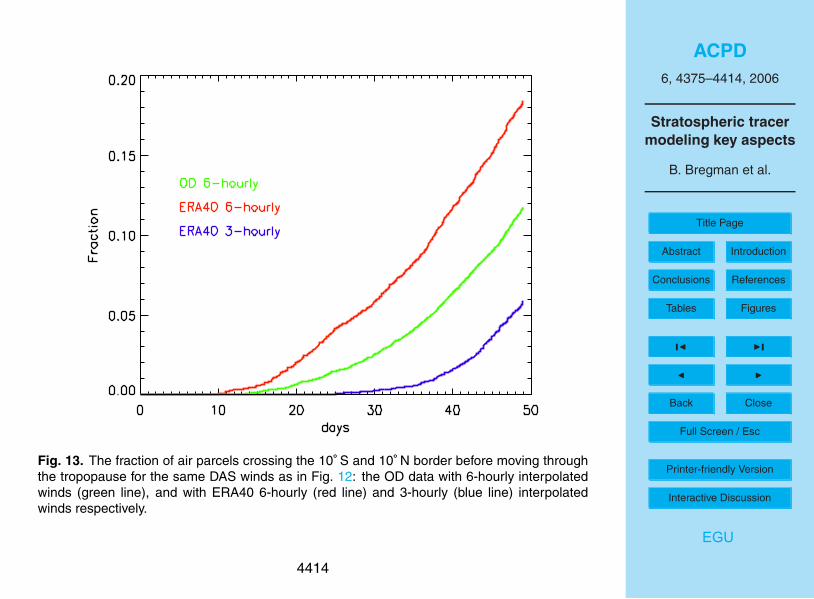
ACPD6, 4375–4414, 2006


B. Bregman et al.

Title Page



Tables Figures

J I

J I

Back Close

Full Screen / Esc



EGU


Fig. 13. The fraction of air parcels crossing the 10◦S and 10◦Nborder before moving through the tropopause for the same DASwinds as in figure 12: the OD data with 6-hourly interpolated winds(green line), and with ERA40 6-hourly (red line) and 3-hourly (blueline) interpolated winds respectively.


Fig. 13. The fraction of air parcels crossing the 10◦ S and 10◦ N border before moving throughthe tropopause for the same DAS winds as in Fig. 12: the OD data with 6-hourly interpolatedwinds (green line), and with ERA40 6-hourly (red line) and 3-hourly (blue line) interpolatedwinds respectively.

4414





Key aspects of stratospheric tracer modeling

Documents

Transcript of Key aspects of stratospheric tracer modeling