(Kernel) Regularized Generalized Canonical Correlation...
57
(Kernel) Regularized Generalized Canonical Correlation Analysis Arthur Tenenhaus Michel Tenenhaus Strasbourg, 17/12/2010
Transcript of (Kernel) Regularized Generalized Canonical Correlation...

(Kernel) Regularized Generalized
Canonical Correlation Analysis
Arthur Tenenhaus
Michel Tenenhaus
Strasbourg, 17/12/2010
References
2
• Paper
Arthur & Michel Tenenhaus
Regularized Generalized CCA
Psychometrika (2011)
• R package
New package RGCCA with initial version 1.0
Title: Regularized Generalized Canonical Correlation Analysis
Version: 1.0
Date: 2010-06-08
Author: Arthur Tenenhaus
Repository: CRAN
Date/Publication: 2010-10-15 14:58:02
More information about RGCCA at CRAN
Path: /cran/new | permanent link

3
Economic inequality and political instability Data from
Russett (1964), in GIFI
Economic inequality
Agricultural inequality
GINI : Inequality of land
distributions
FARM : % farmers that own half
of the land (> 50)
RENT : % farmers that rent all
their land
Industrial development
GNPR : Gross national product
per capita ($ 1955)
LABO : % of labor force
employed in agriculture
Political instabilityINST : Instability of executive (45-61)
ECKS : Nb of violent internal war
incidents (46-61)
DEAT : Nb of people killed as a result of
civic group violence (50-62)
D-STAB : Stable democracy
D-UNST : Unstable democracy
DICT : Dictatorship

Economic inequality and political instability
(Data from Russett, 1964)
Gini Farm Rent Gnpr Labo Inst Ecks Deat Demo
Argentine 86.3 98.2 32.9 374 25 13.6 57 217 2
Australie 92.9 99.6 3.27 1215 14 11.3 0 0 1
Autriche 74.0 97.4 10.7 532 32 12.8 4 0 2
France 58.3 86.1 26.0 1046 26 16.3 46 1 2
Yougoslavie 43.7 79.8 0.0 297 67 0.0 9 0 3
X1 X2 X3
Agricultural inequality
GINI : Inequality of land distributions
FARM : % farmers that own half of the land (> 50)
RENT : % farmers that rent all their land
Industrial development
GNPR : Gross national product per capita ($, 1955)
LABO : % of labor force employed in agriculture
Political instability
INST : Instability of executive (45-61)
ECKS : Nb of violent internal war incidents (46-61)
DEAT : Nb of people killed as a result of civic group violence (50-62)
DEMO : Stable democracy (1), Unstable democracy (2) or Dictatorship (3)

5
Structural relation between blocks
GINI
FARM
RENT
GNPR
LABO
Agricultural inequality (X1)
Industrial
development (X2)
ECKS
DEAT
D-STB
D-INS
INST
DICT
Political
instability (X3)
1
2
3
C13 = 1
C23 = 1
C12 = 0
6
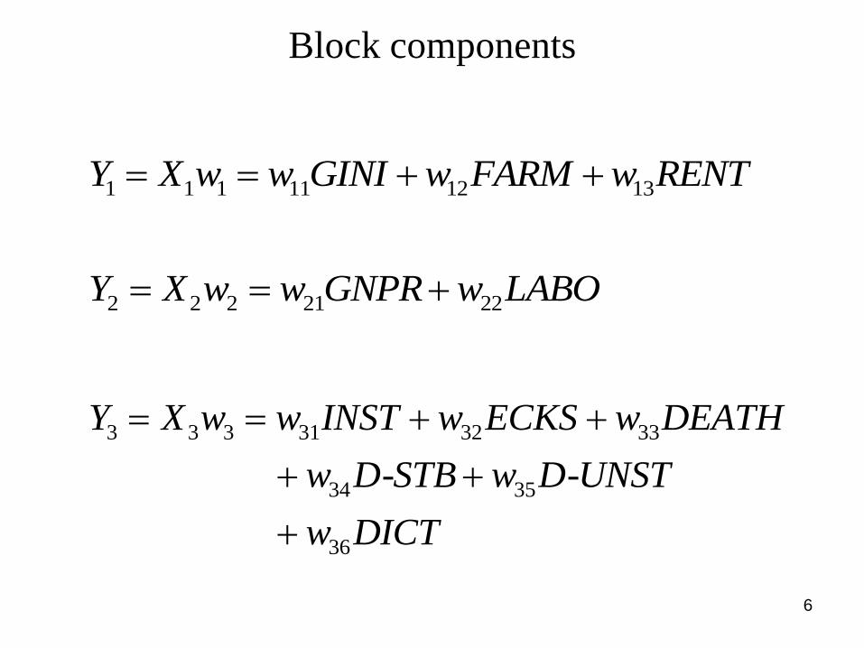
Block components
1 1 1 11 12 13Y X w w GINI w FARM w RENT
2 2 2 21 22Y X w w GNPR w LABO
3 3 3 31 32 33
34 35
36
- -
Y X w w INST w ECKS w DEATH
w D STB w D UNST
w DICT

77
SUMCOR (Horst, 1961) ,
( , )jk j j k k
j k
Max c Cor X w X w
SSQCOR (Mathes, 1993, Hanafi, 2004) 2
,
( , )jk j j k k
j k
Max c Cor X w X w
SABSCOR (Mathes, 1993, Hanafi, 2004) ,
| ( , ) |jk j j k k
j k
Max c Cor X w X w
MAXDIFF (Van de Geer, 1984)
[SUMCOV] All 1
,
( , )j
jk j j k kw
j k
Max c Cov X w X w
MAXDIFF B (Hanafi & Kiers, 2006)
[SSQCOV]
2
All 1,
( , )j
jk j j k kw
j k
Max c Cov X w X w
SABSCOV (Krämer, 2007) All 1
,
( , )j
jk j j k kw
j k
Max c Cov X w X w
Some modified multi-block methods
cjk = 1 if blocks are linked, 0 otherwise and cjj = 0
GENERALIZED CANONICAL CORRELATION ANALYSIS
GENERALIZED CANONICAL COVARIANCE ANALYSIS

8
SUMCOR ,
All ( ) 1( , )jk j j k k
j jj kVar X w
Max c Cov X w X w
SSQCOR 2
,All ( ) 1
( , )jk jj j
j k k
j kVar X w
Max c Cov X w X w
SABSCOR ,
All ( ) 1| ( , ) |jk j j k k
jj kjVar X wMax c Cov X w X w
SUMCOV ,All 1
( , )jk j j k k
j j kwMax c Cov X w X w
SSQCOV 2
,All 1 ( , )j
j
k j j k k
j kwMax c Cov X w X w
SABSCOV ,All 1
( , )jk j j k k
j j kwMax c Cov X w X w
Covariance-based criteria
cjk = 1 if blocks are linked, 0 otherwise and cjj = 0

9
Starting point : RGGCA (for linear dependence)
9
argmax𝐚1 ,𝐚2 ,…,𝐚𝐽
𝑐𝑗𝑘 g cov 𝐗𝑗𝐚𝑗 ,𝐗𝑘𝐚𝑘
𝐽
𝑗≠𝑘
1 − 𝜏𝑗 var 𝐗𝑗𝐚𝑗 + 𝜏𝑗 𝐚𝑗 2
= 1, 𝑗 = 1,… , 𝐽 Subject to the constraints
and:
identity (Horst sheme)
square (Factorial scheme)
abolute value (Centroid scheme)
g
Shrinkage constant between 0 and 1j
otherwise 0
connected is and if 1 kj XXjkcwhere:
A monotone convergent algorithm
related to this optimization problem
will be described.

GINI
FARM
RENT
GNPR
LABO
Agricultural inequality (X1)
Industrial development (X2)
ECKS
DEAT
D-STB
D-INS
INST
DICT
Political instability (X3)
Agr.
ineq.
Ind.
dev.
Pol.
inst.
C13 = 1
C23 = 1
C12 = 0
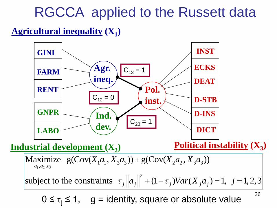
RGCCA applied to the Russett data
10
1 2 3
1 1 3 3 2 2 3 3, ,
2
Maximize g(Cov( , )) g(Cov( , ))
subject to the constraints (1 ) ( ) 1, 1,2,3
a a a
j j j j j
X a X a X a X a
a Var X a j
0 ≤ j ≤ 1, g = identity, square or absolute value

11
Construction of monotone convergent algorithms for
these criteria
• Construct the Lagrangian function related to the
optimization problem.
• Cancel the derivative of the Lagrangian function with
respect to each wj.
• Use the Wold’s procedure to solve the stationary
equations ( Gauss-Seidel algorithm).
• This procedure is monotonically convergent: the
criterion increases at each step of the algorithm.
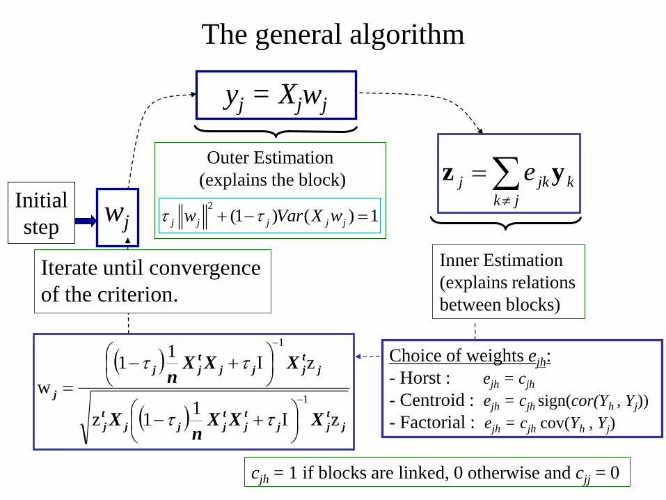
12
wjInitial
step
yj = Xjwj
Outer Estimation
(explains the block)
2
(1 ) ( ) 1j j j j jw Var X w
The general algorithm
Iterate until convergence
of the criterion.
Choice of weights ejh:
- Horst : ejh = cjh
- Centroid : ejh = cjh sign(cor(Yh , Yj))
- Factorial : ejh = cjh cov(Yh , Yj)
cjh = 1 if blocks are linked, 0 otherwise and cjj = 0
Inner Estimation
(explains relations
between blocks)
k
jk
jkj e yz
j
t
jj
t
j
t
jjj
t
j
j
t
jjj
t
jj
j
XXXn
X
XXXn
zI1
1z
zI1
1
w1
1

1313
PLS regression: Wold S., Martens & Wold H. (1983): The multivariate calibration problem in chemistry solved by the PLS method. In Proc.
Conf. Matrix Pencils, Ruhe A. & Kåstrøm B. (Eds), March 1982, Lecture Notes in Mathematics, Springer Verlag,
Heidelberg, p. 286-293.
Redundancy analysis : Barker M. & Rayens W. (2003): Partial least squares for discrimination, Journal of Chemometrics, 17, 166-173.
Regularized CCA : Vinod H. D. (1976): Canonical ridge and econometrics of joint production. Journal of Econometrics, 4, 147–166.
Inter-battery factor Tucker L.R. (1958): An inter-battery method of factor analysis, Psychometrika, vol. 23, n°2, pp. 111-136.
Analysis:
MCOA : Chessel D. and Hanafi M. (1996): Analyse de la co-inertie de K nuages de points. Revue de Statistique Appliquée, 44, 35-60
SSQCOV: Hanafi M. & Kiers H.A.L. (2006): Analysis of K sets of data, with differential emphasis on agreement between and within
sets, Computational Statistics & Data Analysis, 51, 1491-1508.
SUMCOR: Horst P. (1961): Relations among m sets of variables, Psychometrika, vol. 26, pp. 126-149.
SSQCOR: Kettenring J.R. (1971): Canonical analysis of several sets of variables, Biometrika, 58, 433-451
MAXDIFF : Van de Geer J. P. (1984): Linear relations among k sets of variables. Psychometrika, 49, 70-94.
PLS path modeling: Tenenhaus M., Esposito Vinzi V., Chatelin Y.-M., Lauro C. (2005): PLS path modeling. Computational Statistics and Data
(mode B) Analysis, 48, 159-205.
Generalized orthogonal Vivien M. & Sabatier R. (2003): Generalized orthogonal multiple co-inertia analysis (-PLS): new multiblock component
multiple co-inertia and regression methods, Journal of Chemometrics, 17, 287-301.
Analysis:
Caroll’s RGCCA : Takane Y., Hwang H. and Abdi H. (2008): Regularized Multiple-set Canonical Correlation Analysis, Psychometrika, 73
(4):753-775
Caroll ‘s GCCA : Carroll, J.D. (1968): A generalization of canonical correlation analysis to three or more sets of variables, Proc. 76th
Conv. Am. Psych. Assoc., pp. 227-228.
special cases of RGCCA (among others)

Method Criterion Constraints
PLS regression 1 1 2 2Maximize Cov( , )X a X a 1 2 1 a a
Canonical
Correlation
Analysis 1 1 2 2Maximize Cor( , )X a X a 1 1 2 2Var( ) Var( ) 1 X a X a
Redundancy
analysis of X1 with
respect to X2
1/ 2
1 1 2 2 1 1
Maximize
Cor( , )Var( )X a X a X a 1
2 2
1
Var( ) 1
a
X a
1 1 2 2Maximize Cov( , )
subject to (1 )Var( ) 1j j j j j
X a X a
a X a
Special cases
14
The two-block case: Regularized CCA
Components X1a1 and
X2a2 are well correlated.
No stability condition
for 2nd component1st component is stable

Method Criterion Comments
PLS regression 1 1 2 2
1 2a a 1Maximize Cov( , )
X a X a
Is favoring too much
stability with respect to
correlation
Canonical Correlation
Analysis 1 1 2 2Maximize Cor( , )X a X a
Is favoring too much
correlation with respect to
stability
1 1 2 2Maximize Cov( , )
subject to (1 )Var( ) 1j j j j j
X a X a
a X a
Special cases
15
The two-block case: Regularized CCA

1 1 2 2Maximize Cov( , )
subject to (1 )Var( ) 1j j j j j
X a X a
a X a
16
Choice of the shrinkage constant j
0 1
Favoring
correlation
Favoring
stability
j
Schäfer and Strimmer (2005) give a formula for an optimal
choice of j.

SUMCOR (Horst, 1961)
SSQCOR (Kettenring, 1971)
SABSCOR (Mathes, 1993, Hanafi, 2004)
MAXDIFF (Van de Geer, 1984)
[SUMCOV]
(MAXDIFF B Hanafi & Kiers, 2006)
[SSQCOV]
SABSCOV (Krämer, 2007)
( ) 1, ,
Cor( , )
j j
j j k kVar X a
j k j k
Max X a X a
2
( ) 1, ,
Cor ( , )
j j
j j k kVar X a
j k j k
Max X a X a
( ) 1, ,
Cor( , )
j j
j j k kVar X a
j k j k
Max X a X a
1, ,
Cov( , )
j
j j k ka
j k j k
Max X a X a
2
1, ,
Cov ( , )
j
j j k ka
j k j k
Max X a X a
1, ,
Cov( , )
j
j j k ka
j k j k
Max X a X a
Special cases of Regularized generalized CCA
RGCCA and Multi-block data analysis
17
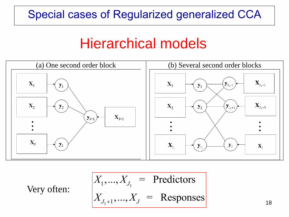
Special cases of Regularized generalized CCA
Hierarchical models
(a) One second order block
(b) Several second order blocks
1
1
1
1
,..., = Predictors
,..., = Responses
J
J J
X X
X X
Very often:
18

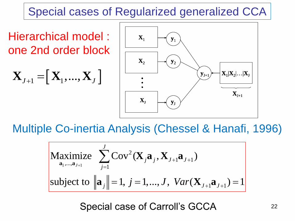
Special cases of Regularized generalized CCA
Hierarchical model : one 2nd order block
Method Criterion Constraints
Hierarchical PLS
regression 1 1
1 1,...,
1
Maximize g(Cov( , ))
J
J
j j J J
j
a a
X a X a 1, 1,..., 1j j J a
Hierarchical
Canonical Correlation
Analysis
1 1
1 1,...,
1
Maximize g(Cor( , ))
J
J
j j J J
j
a a
X a X a Var( ) 1, 1,..., 1j j j J X a
Hierarchical
Redundancy analysis
of the jX ’s with
respect to 1J X
1 1,...,
1/ 2
1 1
1
Maximize
g(Cor( , )Var( ) )
J
J
j j J J j j
j
a a
X a X a X a 1 1
1, 1,...,
Var( ) 1
j
J J
j J
a
X a
Hierarchical
Redundancy analysis
of 1J X with respect
to the jX ’s
1 1,...,
1/ 2
1 1 1 1
1
Maximize
g(Cor( , )Var( ) )
J
J
j j J J J J
j
a a
X a X a X a 1
Var( ) 1, 1,...,
1
j j
J
j J
X a
a
g = identity, square or absolute value
Stable predictors and good prediction
Good predictors and stable response
19

Special cases of Regularized generalized CCA
Hierarchical model : one 2nd order block
Factorial scheme : g = square function
Concordance analysis (Hanafi & Lafosse, 2001)
2
1 1 1
1
Maximize Cov ( , )
subject to 1, 1,..., 1
J
j j j J J J
j
t
j j j j J
X M b X M b
b M b
The previous methods are found again for
the metrics Mj equal to identity or Mahalanobis
20

Special cases of Regularized generalized CCA
X1
X2
XJ
X1|X2|…|XJ
y1
y2
yJ
yJ+1
XJ+1
X1
X2
XJ
X1|X2|…|XJ
y1
y2
yJ
yJ+1
XJ+1
Method Criterion Constraints
SUMCOR
(Horst, 1961)
1 1
1 1,...,
1
Maximize Cor( , )J
J
j j J J
j
a a
X a X a
or
1 1
1 1,...,
1
Maximize Cor( , )J
J
j j J J
j
a a
X a X a
Var( ) 1, 1,..., 1j j j J X a
Generalized CCA
(Carroll, 1968a,b)
1
1 1
1
2
1 1,...,
1
2
1 1
1
Maximize Cor ( , )
Cov ( , )
J
J
j j J J
j
J
j j J J
j J
a aX a X a
X a X a
1
1
Var( ) 1, 1,..., , 1
1, 1,...,
j j
j
j J J
j J J
X a
a
Hierarchical model :
one 2nd order block
1 1,...,J J X X X
21
Special cases of Regularized generalized CCA
X1
X2
XJ
X1|X2|…|XJ
y1
y2
yJ
yJ+1
XJ+1
X1
X2
XJ
X1|X2|…|XJ
y1
y2
yJ
yJ+1
XJ+1
Hierarchical model :
one 2nd order block
1 1,...,J J X X X
Multiple Co-inertia Analysis (Chessel & Hanafi, 1996)
1 1
2
1 1,...,
1
1 1
Maximize Cov ( , )
subject to 1, 1,..., , ( ) 1
J
J
j j J J
j
j J Jj J Var
a aX a X a
a X a
Special case of Carroll’s GCCA 22

Special cases of Regularized generalized CCA
Hierarchical model : several 2nd order blocks
cjk = 1 if response block Xk is connected to predictor block Xj,
= 0 otherwise23

Special cases of Regularized generalized CCA
Hierarchical model : several 2nd order blocks
1
11
,...,1 1
2
Maximize c g(Cov( , ))
subject to the constraints: (1 )Var( ) 1, 1,...,
J
J J
jk j j k k
j k J
j j j j j j J
a aX a X a
a X a
g = identity, square or absolute value 24

Special cases of Regularized generalized CCA
Generalized orthogonal multiple co-inertia analysis
(Vivien & Sabatier, 2003)
1
11
,...,1 1
Maximize Cov( , )
subject to the constraints: 1, 1,...,
J
J J
j j k k
j k J
j j J
a a
X a X a
a
25
GINI
FARM
RENT
GNPR
LABO
Agricultural inequality (X1)
Industrial development (X2)
ECKS
DEAT
D-STB
D-INS
INST
DICT
Political instability (X3)
Agr.
ineq.
Ind.
dev.
Pol.
inst.
C13 = 1
C23 = 1
C12 = 0
RGCCA applied to the Russett data
26
1 2 3
1 1 3 3 2 2 3 3, ,
2
Maximize g(Cov( , )) g(Cov( , ))
subject to the constraints (1 ) ( ) 1, 1,2,3
a a a
j j j j j
X a X a X a X a
a Var X a j
0 ≤ j ≤ 1, g = identity, square or absolute value

Monotone convergence of the algorithm
27
2828
Weight
.66
.74
.11
.69
-.72
Cov
1.00
-1.69
.44
.50
-.55
.46
.17
Weight
.66
.74
.11
.69
-.72
Cov
1.00
-1.69
.44
.50
-.55
.46
.17
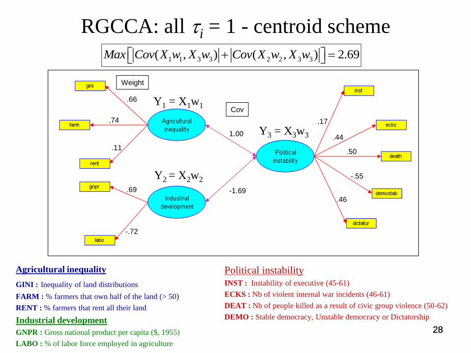
RGCCA: all i = 1 - centroid scheme
1 1 3 3 2 2 3 3( , ) ( , ) 2.69Max Cov X w X w Cov X w X w
Agricultural inequality
GINI : Inequality of land distributions
FARM : % farmers that own half of the land (> 50)
RENT : % farmers that rent all their land
Industrial development
GNPR : Gross national product per capita ($, 1955)
LABO : % of labor force employed in agriculture
Political instability
INST : Instability of executive (45-61)
ECKS : Nb of violent internal war incidents (46-61)
DEAT : Nb of people killed as a result of civic group violence (50-62)
DEMO : Stable democracy, Unstable democracy or Dictatorship
Y1 = X1w1
Y2 = X2w2
Y3 = X3w3
29
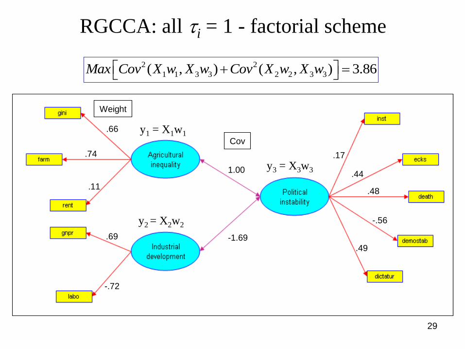
RGCCA: all i = 1 - factorial scheme
Weight
.66
.74
.11
.69
-.72
Cov
1.00
-1.69
.44
.48
-.56
.49
.17
Weight
.66
.74
.11
.69
-.72
Cov
1.00
-1.69
.44
.48
-.56
.49
.17
y1 = X1w1
y2 = X2w2
y3 = X3w3
2 2
1 1 3 3 2 2 3 3( , ) ( , ) 3.86Max Cov X w X w Cov X w X w

30
RGCCA: - centroid scheme𝜏𝑖 = 𝜏𝑖∗
Weight
.66
.74
.11
.69
-.72
Cov
1.00
-1.69
.44
.50
-.55
.46
.17
Weight
.66
.74
.11
.69
-.72
Cov
1.00
-1.69
.44
.50
-.55
.46
.17
𝝉𝟐 = 𝟎.𝟎𝟕
𝝉𝟏 = 𝟎.𝟏𝟒
𝝉𝟑 = 𝟎.𝟏𝟐
.83
.85
-.07
.92
-.97
.25
.69
.66
-.95
.76
cor = .54
cor= -.78
correlation
y1 = X1w1
y2 = X2w2
y3 = X3w3

Generalized Barker & Rayens PLS-DA
1 = 2 = 1 and 3 = 0 - Factorial scheme
2 2
1 1 3 3 1 1 2 2 3 3 2 2( , )* ( ) ( , )* ( ) 1.39Max Cor X w X w Var X w Cor X w X w Var X w
Weight
.62
.75
.22
.67
-.74
Cov
.55
-1.04
.39
-.72
Weight
.62
.75
.22
.67
-.74
Cov
.55
-1.04
.39
-.72
Weight
.62
.75
.22
.67
-.74
Cov
.55
-1.04
.39
-.72

Generalized Barker & Rayens PLS-DA
Agricultural inequality
Industr
ial develo
pm
ent
These countries
have known a
period of
dictatorship
after 1964.
3333
-1.5 -1 -0.5 0 0.5 1 1.5-1.5
-1
-0.5
0
0.5
1
1.5
0 0.5 1 1.5 2 2.5-0.5
0
0.5
1
1.5
2
2.5
-1.5 -1 -0.5 0 0.5 1 1.5-0.5
0
0.5
1
1.5
2
2.5
X
Y
X
Y
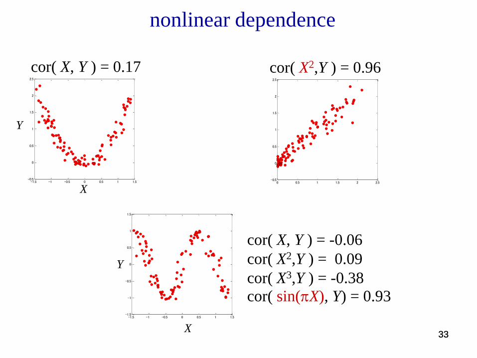
cor( X, Y ) = 0.17 cor( X2,Y ) = 0.96
cor( X, Y ) = -0.06
cor( X2,Y ) = 0.09
cor( X3,Y ) = -0.38
cor( sin(pX), Y) = 0.93
nonlinear dependence

RGCCA in action : toy example
X11 with block X2 = [X21, X22]
Simulated data : • Number of observations : 500
• Number of blocks : 2 (2 variables per block)
X12 with block X2 = [X21, X22]
35
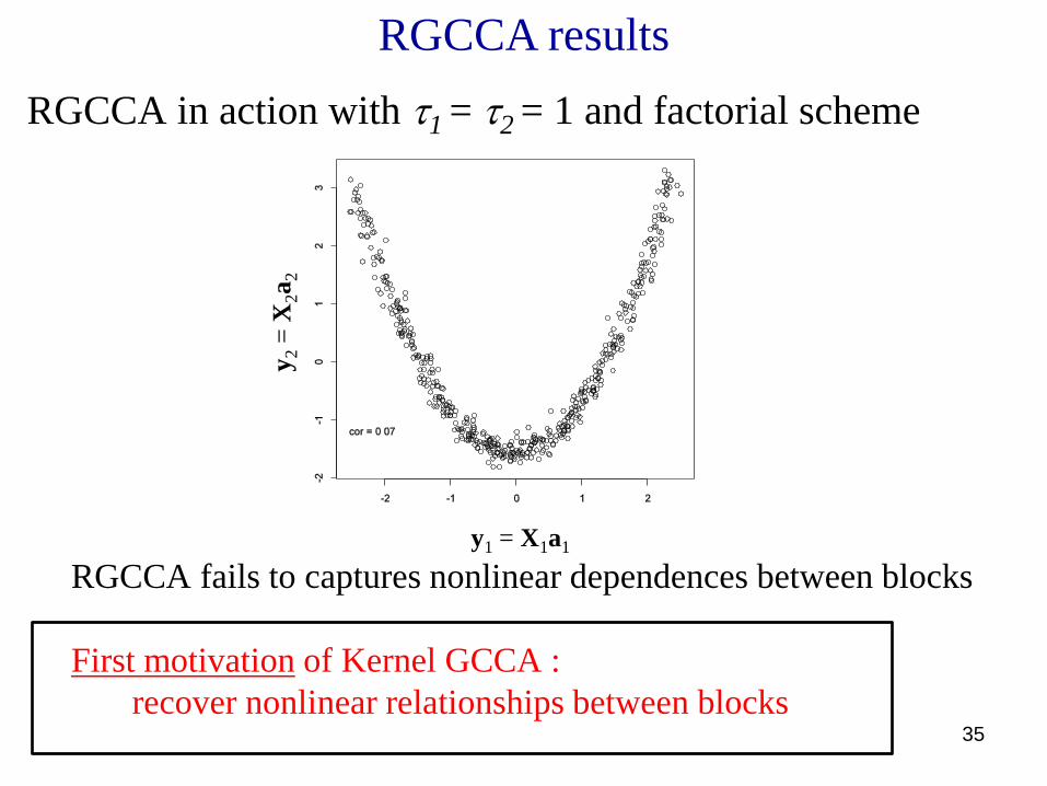
RGCCA results
RGCCA fails to captures nonlinear dependences between blocks
First motivation of Kernel GCCA :
recover nonlinear relationships between blocks
RGCCA in action with 1 = 2 = 1 and factorial scheme
y1 = X1a1
y2
= X
2a
2

363636
Glioma Cancer Data(From the Department of Pediatric Oncology of the Gustave Roussy Institute, 2009)
Gene 1 Gene 2 … Gene 27982 CGH1 … CGH 3268 Outcome
Patient 1 0.18 -0.21 -0.73 0.00 -0.55 X
Patient 2 1.15 -0.45 0.27 -0.30 0.00 X
Patient 3 1.35 0.17 0.22 0.33 0.64 Y
Patient 36 1.39 0.18 -0.17 0.00 0.43 Z
Transcriptomic data (X1)
CGH data (X2)
outcome (X3)

37373737
RGCCA in action in a very high dimensional
blocks settings
• Requires to invert J matrices
Here p1 = 27982, p2 = 3268 and p3 = 2
Second motivation of Kernel GCCA :
Capable of dealing with very high dimensional blocks settings
𝐌𝑗 = 1 − 𝜏𝑗 1
𝑛𝐗𝑗𝑡𝐗𝑗 + 𝜏𝑗 𝐈𝑝𝑗 𝑗 = 1,… , 𝐽
𝐌𝑗 ∈ ℝ𝑝𝑗×𝑝𝑗 𝑗 = 1,… , 𝐽 where

38
what we have …
• A set of n observations characterized by different point of view
X1 X2 X3
• Links between blocks that are assumed to be connected
x3
x2
x6
x1
x4
x5
x7
x8
x3
x2
x6
x1
x4
x5
x7x8
x7
x5
x2x3
x6 x8x1
x4E1
X1 X2
X3
E2 E3

x3
x2
x6
x1
x4
x5
x7
x8
Kernel GCCA: an idea
Ej
j
Hj
j(x1)
j(x6)
j(x7)j(x3)
j(x5)
j(x8)
j(x4)
j(x2)
Apply RGCCA on the feature spaces H1,…, HJ
• How to choose 1, … J → kernel method
where kj: Ej × Ej is a positive definite kernel function and Hj
associated reproducing kernel Hilbert space.
𝑗 𝑥 = 𝑘𝑗 (. , 𝑥) 𝑗 = 1,… , 𝐽

Kernel GCCA (two-block case)
𝑦1𝑖 = 𝑓1 ,Φ1 𝑥1 𝑖 and 𝑦2𝑖 = 𝑓2,Φ2(𝑥2
𝑖 )
For any two directions H1 and H2, define the projections
y1i of on f1 and y2i of on f2 by:Φ1 𝑥1 𝑖 Φ2 𝑥2
𝑖
𝑓1 ∈ 𝑓2 ∈
The goal of KGCCA (two-block case) is to find H1 and H2
that maximize the following optimization problem:
argmax𝑓1∈𝐻1 ,𝑓2∈𝐻2
cov 𝐲1,𝐲2
1 − 𝜏𝑗 var 𝐲𝑗 + 𝜏𝑗 𝑓𝑗 2
= 1, 𝑗 = 1,2 s.c.
𝑓1 ∈ 𝑓2 ∈
Hj

41
It is always possible to express fj as follows: 𝑓𝑗 = 𝛼𝑗(𝑘)
𝑛
𝑘=1
Φ𝑗 𝑥𝑗 𝑘
𝐊𝑗 𝑘𝑖= 𝑘 𝑥𝑗
𝑘 ,𝑥𝑗 𝑖 = Φ𝑗 𝑥𝑗
𝑘 ,Φ𝑗 𝑥𝑗 𝑖
Kernel GCCA (two-block case)
Let us note Kj the n n kernel matrix defined by:
𝑦𝑗𝑖 = 𝑓𝑗 ,Φ𝑗 𝑥𝑗 𝑖 = 𝛼𝑗
𝑘
𝑛
𝑘=1
Φ𝑗 𝑥𝑗 𝑘
,Φ𝑗 𝑥𝑗 𝑖
𝐲𝒋 = 𝐊𝒋𝛂𝒋
We deduce that can be re-expressed as follows:𝑦𝑗𝑖
We deduce that is defined by:𝐲𝒋

42
argmax𝛼1 ,𝛼2
1
𝑛𝛂1𝑡𝐊1𝐊2𝛂2
1 − 𝜏𝑗 1
𝑛𝛂𝑗𝑡𝐊𝑗
2𝛂𝐣 + 𝜏𝑗𝛂𝑗𝑡𝐊𝑗𝛂𝑗 = 1 𝑗 = 1, 2 s.c.
can be write down only in terms of kernel matrices as follows:
Kernel GCCA (two-block case)
argmax𝑓1∈𝐻1 ,𝑓2∈𝐻2
cov 𝐲1,𝐲2
1 − 𝜏𝑗 var 𝐲𝑗 + 𝜏𝑗 𝑓𝑗 2
= 1, 𝑗 = 1,2 s.c.Hj
Then the previous optimization problem:
4343
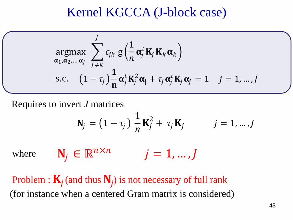
Kernel KGCCA (J-block case)
argmax𝛂1 ,𝛂2 ,…,𝛂𝐽
𝑐𝑗𝑘
𝐽
𝑗≠𝑘
g 1
𝑛𝛂𝑗𝑡𝐊𝑗𝐊𝑘𝛂𝑘
1 − 𝜏𝑗 𝟏
𝐧𝛂𝑗𝑡𝐊𝑗
2𝛂𝐣 + 𝜏𝑗𝛂𝑗𝑡𝐊𝑗𝛂𝑗 = 1 𝑗 = 1,… , 𝐽 s.c.
Requires to invert J matrices
𝐍𝑗 = 1 − 𝜏𝑗 1
𝑛𝐊𝑗
2+ 𝜏𝑗𝐊𝑗 𝑗 = 1,… , 𝐽
𝐍𝑗 ∈ ℝ𝑛×𝑛 𝑗 = 1,… , 𝐽 where
Problem : (and thus ) is not necessary of full rank
(for instance when a centered Gram matrix is considered)
𝐊𝑗 𝐍𝑗

4444444444
(incomplete) Cholesky Decomposition
• Find a lower triangular matrix such that
𝐑𝑗 ∈ ℝrank 𝐊𝑗 ×𝑛 where
𝐑𝑗 𝐊𝑗 = 𝐑𝑗𝑡𝐑𝑗
argmax𝛂1 ,𝛂2 ,…,𝛂𝐽
𝑐𝑗𝑘
𝐽
𝑗≠𝑘
g 1
𝑛𝛂𝑗𝑡𝐑𝑗
𝑡𝐑𝑗𝐑𝑘𝑡 𝐑𝑘𝛂𝑘
1 − 𝜏𝑗 1
𝑛𝛂𝑗𝑡𝐑𝑗
𝑡𝐑𝑗𝐑𝑗𝑡𝐑𝑗𝛂𝑗 + 𝜏𝑗𝛂𝑗
𝑡𝐑𝑗𝑡𝐑𝑗𝛂𝑗 = 1, 𝑗 = 1,… , 𝐽 s.c.

45
argmax𝐰1 ,𝐰2 ,…,𝐰𝐽
𝑐𝑗𝑘
𝐽
𝑗 ,𝑘
g 1
𝑛𝐰𝑗
𝑡𝐑𝑗𝐑𝑘𝑡 𝐰𝑘
1 − 𝜏𝑗 1
𝑛𝐰𝑗
𝑡𝐑𝑗𝐑𝑗𝑡𝐰𝑗 + 𝜏𝑗𝐰𝑗
𝑡𝐰𝑗 = 1, 𝑗 = 1,… , 𝐽 s.c.
𝐰𝑗 = 𝐑𝑗𝛂𝑗
The KGCCA optimization problem
Apply the initial algorithm of RGCCA on to obtain the
Latent variables outer estimation.
In the glioma Cancer Data :
𝐑1𝑡 ,…, 𝐑𝐽
𝑡
𝐗1 ∈ ℝ36×27982 → 𝐑𝟏𝐭 ∈ ℝ36×35
𝐗2 ∈ ℝ36×3268 → 𝐑2𝑡 ∈ ℝ36×34

4646
Construction of monotone convergent algorithms for
these criteria
• Construct the Lagrangian function related to the
optimization problem.
• Cancel the derivative of the Lagrangian function with
respect to each .
• Use the RGCCA procedure to solve the stationary
equations.
• This procedure is monotonically convergent: the
criterion increases at each step of the algorithm.
𝐰𝑗

4747
The Kernel GCCA algorithm
j
t
jj wRy
Outer Estimation
(explains the block)
1n
11 jrankj
t
jjj
t
j j
wIRRw KInitial
step jw
jjj
t
jjj
t
j
t
j
jjj
t
jjj
j
j
j
n
n
zRIRR1
1Rz
zRIRR1
1
w1
)K(rank
1
)K(rank
Iterate until
convergence
of the criterion
cjk = 1 if blocks are linked, 0 otherwise and cjj = 0
Inner
Estimation
(explains
relation
between
block)
k
jk
jkj e yz
Choice of weights ejh:
- Horst :
- Centroid :
- Factorial :
jkjk ce
kjjkjk ce yy ,corsign
kjjkjk ce yy ,cov
48
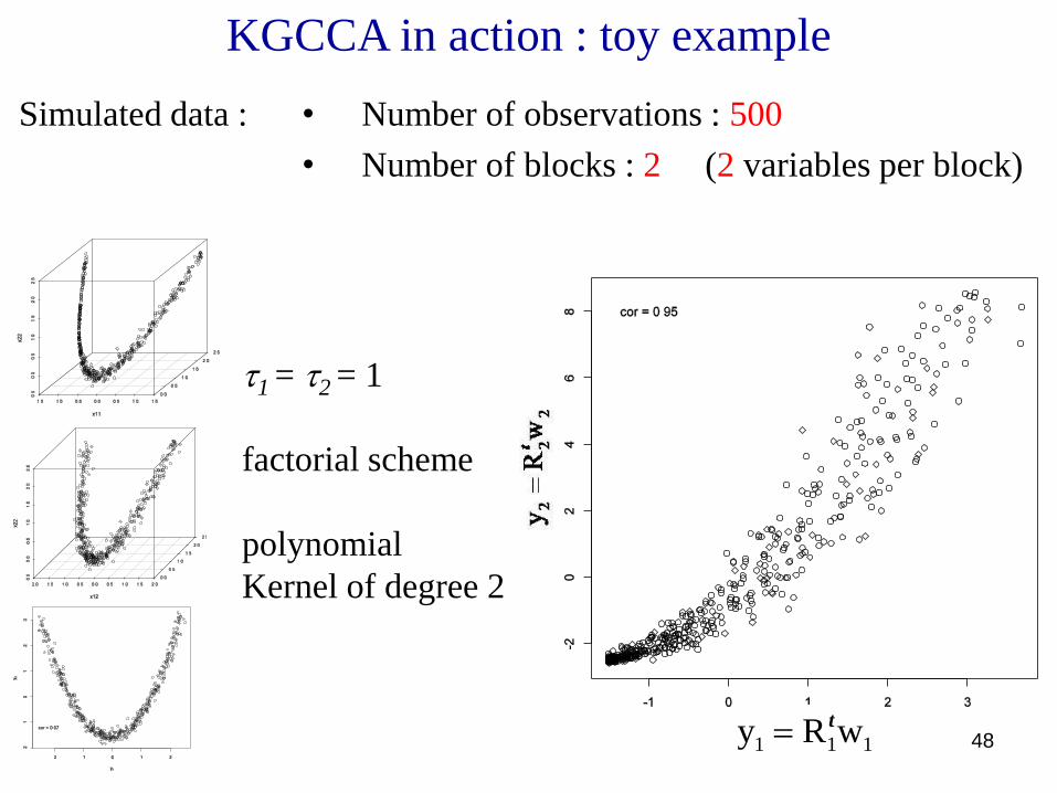
KGCCA in action : toy example
1 = 2 = 1
factorial scheme
polynomial
Kernel of degree 2
Simulated data : • Number of observations : 500
• Number of blocks : 2 (2 variables per block)
111 wRy t

49
RGCCA results (factorial scheme, j =1)

50
KGCCA results (factorial scheme, j =1, spline kernel)
32 yx3
1yx
2
yxyxxyxy1yxk ),min(),min(),min(),(

5151
Glioma Cancer Data(From the Department of Pediatric Oncology of the Gustave Roussy Institute, 2009)
Gene 1 Gene 2 … Gene 27982 CGH1 … CGH 3268 Outcome
Patient 1 0.18 -0.21 -0.73 0.00 -0.55 X
Patient 2 1.15 -0.45 0.27 -0.30 0.00 X
Patient 3 1.35 0.17 0.22 0.33 0.64 Y
Patient 36 1.39 0.18 -0.17 0.00 0.43 Z
Transcriptomic data (X1)
CGH data (X2)
outcome (X3)

5252
Glioma Cancer : from a RGCCA point of view
Transcriptomic data (X1)
CGH data (X2)
outcome (X3)C13=1
C23=1
C12=1
CGH1
…
CGH3962
Gene1
…
Gene27982 X/Y/Z
2
1
3

53
Glioma Cancer : from a KGCCA point of view
Transcriptomic data ( )
CGH data ( )
1
2
C13=1
C23=1
C12=1
V21
…
V2,34
V11
…
V1,35
(1 = 1)
(2 = 1)
2
Outcome ( )
X
Y
(1 = 1)
𝐑3𝑡
𝐑1𝑡
𝐑2𝑡
Factorial scheme, linear kernel, 1 = 1

54
Monotone convergence of the KGCCA algorithm

55
y1 versus y2 (learning phase)

56
y1 versus y2 (leave one out phase)

57
Redundancy analysis(2,3) : Barker M. & Rayens W. (2003): Partial least squares for discrimination, Journal of Chemometrics, 17, 166-173.
Caroll GCCA : Carroll, J.D. (1968): A generalization of canonical correlation analysis to three or more sets of variables,
Proc. 76th Conv. Am. Psych. Assoc., pp. 227-228.
MCOA : Chessel D. and Hanafi M. (1996): Analyse de la co-inertie de K nuages de points. Revue de Statistique Appliquée, 44, 35-60
SSQCOV: Hanafi M. & Kiers H.A.L. (2006): Analysis of K sets of data, with differential emphasis on agreement
between and within sets, Computational Statistics & Data Analysis, 51, 1491-1508.
SUMCOR(4): Horst P. (1961): Relations among m sets of variables, Psychometrika, vol. 26, pp. 126-149.
SSQCOR: Kettenring J.R. (1971): Canonical analysis of several sets of variables, Biometrika, 58, 433-451
Caroll’s RGCCA : Takane Y., Hwang H. and Abdi H. (2008): Regularized Multiple-set Canonical Correlation Analysis, Psychometrika, 73 (4):753-775
PLS path modeling: Tenenhaus M., Esposito Vinzi V., Chatelin Y.-M., Lauro C. (2005): PLS path modeling. Computational Statistics and Data Analysis,
48, 159-205.
Inter-battery factor Tucker L.R. (1958): An inter-battery method of factor analysis, Psychometrika, vol. 23, n°2, pp. 111-136.
Analysis(5):
MAXDIFF : Van de Geer J. P. (1984): Linear relations among k sets of variables. Psychometrika, 49, 70-94.
Regularized CCA : Vinod H. D. (1976): Canonical ridge and econometrics of joint production. Journal of Econometrics, 4, 147–166.
Generalized orthogonal Vivien M. & Sabatier R. (2003): Generalized orthogonal multiple co-inertia analysis (-PLS): new multiblock component and
multiple co-inertia regression methods, Journal of Chemometrics, 17, 287-301.
Analysis:
PLS regression(1): Wold S., Martens & Wold H. (1983): The multivariate calibration problem in chemistry solved by the PLS method. In Proc. Conf.
Matrix Pencils, Ruhe A. & Kåstrøm B. (Eds), March 1982, Lecture Notes in Mathematics, Springer Verlag, Heidelberg, p. 286-293.
As conclusion: special cases of KGCCA
(1) Rosipal R., Trejo L.J., Kernel Partial Least Squares Regression in Reproducing Kernel Hilbert space, Journal of Machine Learning Research, 2:97- 123, 2001.
(2) Rosipal R., Trejo L.J., Matthews B. Kernel PLS-SVC for Linear ans Nonlinear Classification, Twentieth International Conference on Machine
Learning, Washington DC, 640-647, 2003.
(3) Takane Y., Hwang H., Regularized linear and kernel redundancy analysis, Computational Statistics & Data Analysis 52: 394–405, 2007
(4) Bach F. R. and Jordan M. I. Kernel independent component analysis. Journal of Machine Learning Research, 3:1–48, 2002.
(5) A. Gretton, A. Smola, O. Bousquet, R. Herbrich, A. Belitski, M. Augath, Y. Murayama, J. Pauls, B. Schölkopf, and N. Logothetis. Kernel constrained
covariance for dependence measurement, AISTATS, volume 10, 2005b.