Kernel PCA for Novelty Detection

Heiko Hoffmann 1,∗

Max Planck Institute for Human Cognitive and Brain Sciences, Amalienstr. 33,

80799 Munich, Germany

Abstract

Kernel principal component analysis (kernel PCA) is a non-linear extension of PCA.This study introduces and investigates the use of kernel PCA for novelty detection.Training data are mapped into an infinite-dimensional feature space. In this space,kernel PCA extracts the principal components of the data distribution. The squareddistance to the corresponding principal subspace is the measure for novelty. Thisnew method demonstrated a competitive performance on two-dimensional syntheticdistributions and on two real-world data sets: handwritten digits and breast-cancercytology.

Key words: Kernel method, novelty detection, PCA, handwritten digit, breastcancer

1 Introduction

Novelty detection is one-class classification—for a review see Markou andSingh [1,2]. In training, a machine learns from ordinary data. Later, usingpreviously unknown data, this machine tries to separate ordinary from novelpatterns.

One-class classification is useful when normal samples are abundant, but ab-normal samples are rare. For example, healthy tissue outweighs malignantcancer. Moreover, if the structure of novel data is obscure, one-class classifica-tion might be advantageous over two-class classification. A machine learningtechnique that works well for data with such characteristics would be of great

∗ Tel.: +44 131 6513437Email address: Heiko.Hoffmann[at]ed.ac.uk (Heiko Hoffmann).

1 Present address: Institute of Perception, Action, and Behavior, School of Infor-matics, University of Edinburgh, EH9 3JZ, UK.

Submitted to Pattern Recognition 14 Nov 2005, revised 27 Jun 2006, accepted 19 Jul 2006

benefit for medical diagnosis, particularly, for the early diagnoses of cancer,which requires the examination of millions of humans [3,4].

For two-class classification, kernel support-vector machines (kernel SVM)proved to be an excellent choice [5]. This non-linear variant of SVM uses thekernel trick: that is, for algorithms in which the data points occur only withinscalar products, the scalar product can be replaced with a kernel function.Thus, the data can be mapped into a higher-dimensional space, a so-calledfeature space, while the algorithm still operates in the original space (see alsosection 2).

Because of the success of SVM, attempts have been made to apply SVM tonovelty detection [6–8]. A SVM needs to separate the data against something.In one-class SVM [6,7], the data are separated from the origin in feature space.Alternatively, the support vector domain description (SVDD) [8] encloses thedata in feature space with a sphere; for radial-basis-function (RBF) kernels,this procedure gives the same result as the one-class SVM [7]. However elegant,these approaches are not satisfactory because for the some training sets, thespace enclosed by the corresponding decision boundaries is too large [9].

A different approach to novelty detection is to generate a simplified modelof the distribution of training data. For linear distributions, principal com-ponent analysis (PCA) is the method of choice, but many interesting distri-butions are non-linear. In the non-linear case, Gaussian mixture models [10],auto-associative multi-layer perceptrons [11], and principal curves and sur-faces [11] have been used. These methods, however, need to solve a non-linearoptimization problem and are thus prone to local minima and sensitive to theinitialization.

This article combines the distribution-modeling approach with kernel tech-niques, which do essentially linear algebra. Here, the distribution of trainingdata is modeled by kernel PCA [12], which computes PCA in the feature space.The novelty of the presented approach is to compute the reconstruction errorin feature space and to use it as a novelty measure. Decision boundaries hereinare iso-potential curves or surfaces of the reconstruction error. Though simple,this method has to my knowledge not been reported before, and it turns outto be a promising novelty detector.

The new method was tested on two-dimensional synthetic distributions andon higher-dimensional real-world data. On the synthetic data, the decisionboundaries can follow smoothly the shape of the distribution of data points.To test the performance quantitatively, an ordinary/ novel classification taskwas carried out on two real-world data sets: handwritten digits and breast-cancer cytology. For both data sets, a receiver-operating-characteristic (ROC)analysis [13,14] demonstrates that the new method does better compared with

2

three alternatives: one-class SVM, standard PCA, and the Parzen windowdensity estimator. All of these methods depend on free parameters. However,a proper parameter choice for kernel PCA leads to a performance that cannotbe matched by any parameter choice for the three other methods.

The remainder of this article is organized as follows. Section 2 briefly reviewsthe kernel PCA algorithm. Section 3 describes the extensions to obtain thenovelty measure. Section 4 reports the experiments. Section 5 shows a discus-sion, and section 6 concludes the article. Appendix A contains a theoreticaltreatment of the reconstruction error with large kernel widths.

2 Kernel PCA

Kernel PCA [5,12] extends standard PCA to non-linear data distributions. Weassume a distribution consisting of n data points xi ∈ IRd. Before performinga PCA, these data points are mapped into a higher-dimensional feature spaceF ,

xi → Φ(xi) . (1)

In this space, standard PCA is performed. The trick herein is that the PCAcan be computed such that the vectors Φ(xi) appear only within scalar prod-ucts [12]. Thus, the mapping (1) can be omitted. Instead, we only work witha kernel function k(x,y), which replaces the scalar product (Φ(x) · Φ(y)).In kernel PCA, an eigenvector V of the covariance matrix in F is a linearcombination of points Φ(xi),

V =n

∑

i=1

αiΦ(xi) , (2)

with

Φ(xi) = Φ(xi) −1

n

n∑

r=1

Φ(xr) . (3)

The vectors Φ(xi) are chosen such that they are centered around the origin inF . The αi are the components of a vector α. It turns out that this vector is aneigenvector of the matrix Kij =

(

Φ(xi)·Φ(xj))

. The length of α is chosen such

that the principal components V have unit length: ||V|| = 1 ⇔ ||α||2 = 1/λ,with λ being the eigenvalue of K corresponding to α. To compute K, wesubstitute Φ according to (3). This substitution gives Kij as a function of thekernel matrix Kij = k(xi,xj):

3

Kij = Kij −1

n

n∑

r=1

Kir −1

n

n∑

r=1

Krj +1

n2

n∑

r,s=1

Krs . (4)

3 Measure for novelty

This section, first, motivates the reconstruction error in feature space, second,considers the simplified case of computing only the distance to the center of thetraining data in F , and, third, shows the computation of the reconstructionerror.

3.1 Motivation

The new method is geometrically motivated and aims at giving lower classifi-cation errors than the one-class SVM. This article focuses on the RBF kernel,particularly, the Gaussian kernel k(x,y) = exp(−||x − y||2/(2σ2)), since thiskernel is the most common for both one-class SVM and SVDD, and experi-ments show that for these methods, the Gaussian kernel is more suitable thanthe polynomial kernel [7–9]. This section illustrates that for RBF kernels, thereconstruction-error decision boundary in F encloses data in general tighterthan the one-class SVM and gives thus a better description of the data (Fig.1).

For RBF kernels, k(x,x) takes the same constant value for all x. Therefore,in F , all Φ(x) lie on a hyper-dimensional sphere S. Figure 1 shows only threedimensions of F , but for RBF kernels, F is infinite-dimensional [5]. However,this illustration is still meaningful since n data points Φ(xi) can span only afinite space U , which is maximally n-dimensional if we include the origin inF . Due to the rotational invariance of the Euclidean norm, also in U , the datalie on a sphere that is embedded in U and centered at the origin.

If we require that all data points are enclosed by the decision boundary (hardmargins), the SVDD encloses all data points in F with a sphere as tight aspossible, and the one-class SVM puts a plane as close as possible to {Φ(xi)}to separate them from the origin. Since the intersection of the SVDD spherewith S equals the intersection of the SVM plane with S, the boundary on Sis the same for both methods [7] (a circle for a three-dimensional U , see Fig.1). This boundary, however, does not tightly enclose the data distribution ifthe data have a multiform variance in F .

In contrast, the reconstruction error takes into account the heterogeneous

4

A B

Φ(x )i

e2

e1

e3

SVDD boundary

Principal component

Reconstruction−error boundaryf1

f2

Φ(x )i

SVDD boundary

One−class SVMboundary

Origin

Reconstruction−error boundary

Fig. 1. Decision boundaries in the feature space of an RBF kernel, comparing one–class SVM, SVDD, and the reconstruction error. (A) The boundaries are illustratedin a three-dimensional feature space. All data points Φ(xi) lie on a sphere. (B)Cross-section through the center of the SVDD sphere and orthogonal to the princi-pal component for the situation in A.

variance of the distribution in F . For multi-variate data, orthogonal to theprincipal subspace, the decision boundary is closer to the data distributionthan the SVDD sphere (Fig.1). In the direction of the principal subspace,also a boundary emerges since S is bending away from the principal subspace(as for the one-class-SVM plane—see Fig. 1 B and Fig. 5). This emergingboundary ensures that the total boundary is closed; this characteristic seems tobe missing for polynomial kernels (Fig. 2, Left), where {Φ(xi)} is not restrictedto a sphere. To conclude, compared with the one-class SVM, for the samenumber of enclosed data points, the reconstruction-error boundary encloses asmaller volume in S.

This illustration already gives an insight for choosing the two free parametersof kernel PCA: the kernel width σ and the number of eigenvectors q. The widthσ must be within a range of optimal values. For small σ, k(xi,xj) ≈ 0 for alli and j with i 6= j. Thus, all Φ(xi) are (almost) orthogonal to each other,and a PCA becomes meaningless. For large σ, the reconstruction error in Fapproaches the reconstruction error for standard PCA (see appendix A). Fur-thermore, q needs to be sufficiently large, because otherwise, the reconstruc-tion error is high for some points within the data distribution. Consequently,the threshold on the novelty measure would be also high leading to a loosedecision boundary (the same holds also for standard PCA). The dependenceon σ and q is studied in the experimental section.

5

3.2 Spherical potential

With no principal components, the reconstruction error reduces to a sphericalpotential field in feature space. All we need is the center of the data in F ,Φ0 = 1/n

∑ni=1

Φ(xi). The potential of a point z in the original space is thesquared distance from the mapping Φ(z) to the center Φ0,

pS(z) = ||Φ(z) − Φ0||2 . (5)

The squared magnitude can be written with kernel functions using the expres-sion for Φ0,

pS(z) = k(z, z) − 2

n

n∑

i=1

k(z,xi) +1

n2

n∑

i,j=1

k(xi,xj) . (6)

All parts of this equation are known. The last term is constant, and cantherefore be omitted. For RBF kernels, the first term is also constant, and thepotential can be simplified to

pS(z) = −2

n

n∑

i=1

k(z,xi) . (7)

This function is up to a multiplicative constant equal to the Parzen windowdensity estimator [15].

3.3 Reconstruction error

As novelty measure, we use the reconstruction error [16] in feature space,

p(Φ) = (Φ · Φ) − (W Φ · W Φ) . (8)

Φ is a vector originating from the center of the distribution in feature space,Φ(z) = Φ(z)−Φ0. Let q be the number of principal components. The matrixW contains the q row vectors Vl. The index l denotes the lth eigenvector,with l = 1 for the eigenvector with the largest eigenvalue.

We need to eliminate Φ in (8), and write the potential as a function of avector z taken from the original space. The projection fl(z) of Φ(z) ontothe eigenvector Vl =

∑ni=1

αliΦ(xi) can be readily evaluated using the kernel

function k,

6

fl(z) = (Φ(z) · Vl) =

[

Φ(z) − 1

n

n∑

r=1

Φ(xr)

]

·

n∑

i=1

αliΦ(xi) −

1

n

n∑

i,r=1

αliΦ(xr)

=n

∑

i=1

αli

k(z,xi) −1

n

n∑

r=1

k(xi,xr)

− 1

n

n∑

r=1

k(z,xr) +1

n2

n∑

r,s=1

k(xr,xs)

. (9)

Here, the second equality uses (3). As a result, p(Φ) can be expressed as

p(Φ) = (Φ · Φ) −q

∑

l=1

fl(z)2 . (10)

The scalar product (Φ · Φ) equals the spherical potential (6). Thus, the ex-pression of the potential p(z) can be further simplified,

p(z) = pS(z) −q

∑

l=1

fl(z)2 . (11)

This is the desired form of the novelty measure in IRd.

The above computation of fl(z) requires n evaluations of the kernel functionfor each z. Since for all l components, the same kernels can be used, the totalnumber of kernel evaluations is also n.

4 Experiments

The decision boundaries for the new method are illustrated using two-dimensionalsynthetic distributions. Furthermore, this method is applied to higher-dimensionaldata, handwritten digits and breast-cancer cytology.

4.1 Methods

The methods section comprises the different data sets, the implementationand evaluation of kernel PCA, and the alternative novelty detectors used forcomparison.

7

4.1.1 Data sets

Kernel PCA for novelty detection was tested on synthetic and real-world datasets. Five synthetic distributions were used: square, square-noise, ring-line-square, spiral, and sine-noise.

Square: The square consists of four lines, 2.2 long and 0.2 wide (Fig. 2).Within the area of these lines, 400 points were randomly distributed withequal probability.

Square-noise: The square-noise was generated by adding to the above distri-bution 50 noise points randomly drawn from the area {(x, y) | x ∈ [0, 3], y ∈[0, 3]}, which surrounds the square (Fig. 5).

Ring-line-square: The ring-line-square distribution is composed of a ringwith an inner diameter of 1.0 and an outer diameter of 2.0, a square with thesize as described above, and a 1.6 long and 0.2 wide line connecting the twoparts (Fig. 3). Within the area of these three parts, 850 points were randomlydistributed with equal probability.

Spiral: The area of the spiral is defined by the set {(x, y) | x = (0.07ϕ +a) cos(ϕ), y = (0.07ϕ + a) sin(ϕ), a ∈ [0, 0.1], ϕ ∈ [0, 6π]}. Within this area,700 points were randomly distributed with equal probability (Fig. 4).

Sine-noise: The sine-noise distribution consists of a sine-wave and surround-ing noise (Fig. 6). In the sine-wave part, 500 points are uniformly distributedalong y = 0.8 sin(2ϕ) with ϕ ∈ [0, 2π]. These points are surrounded by 200points that were distributed randomly with equal probability in the rectangle{(x, y) | x ∈ [0, 2π], y ∈ [−1.5, 1.5]}.

Two real-world data sets were used: handwritten digits and breast-cancer data.

Digit 0: The digits were obtained from the MNIST digit database [17]. Theoriginal 28 × 28 pixels images are almost binary (see Fig. 11). Thus, the dig-its occupy only the corners of a 784-dimensional hyper-cube. To get a morecontinuous distribution of digits, the original images were blurred and sub-sampled down to 8 × 8 pixels. The MNIST database is split into training setand test set. To train the novelty detectors, the first 2 000 ‘0’ digits from thetraining set were used. For the 0/not-0 classification task, from the test set,all 980 ‘0’ digits were used together with the first 109 samples from each otherdigit.

Cancer: The breast-cancer data were obtained from the UCI machine-learningrepository [18]. These data were collected by Dr. William H. Wolberg at theUniversity of Wisconsin Hospitals in Madison [19]. The patterns in this dataset belong to two classes: benign and malignant. Each pattern consists of nine

8

cytological characteristics such as, for example, the uniformity of cell size.Each of these characteristics is graded with an integer value from 1 to 10,with 1 being typical benign. The database contains some patterns with miss-ing attributes, these patterns were removed before further processing. Theremaining patterns were scaled to have unit variance in each dimension. Toavoid numerical errors because of the discrete values, a uniform noise fromthe interval [−0.05, 0.05] was added to each value. The novelty detectors weretrained on the first 200 benign samples. The remaining samples were used fortesting: 244 benign and 239 malignant.

4.1.2 Kernel PCA implementation and evaluation

Kernel PCA was computed on all data points of each distribution. Unlessotherwise noted, a Gaussian kernel with width σ was used. Exploratory testswith two other RBF kernels, the ‘multi-quadratic’ and the ‘inverse multi-quadratic’ [5], gave similar optimal results. However, since the Gaussian kernelis commonly used for the one-class SVM, the SVDD, and the Parzen density,this kernel is the only RBF kernel presented here.

The eigenvectors α of K were extracted using the routine ‘dsyevx’ from thelinear algebra package LAPACK. This package is based on BLAS, a stan-dard for basic linear algebra computations. Both BLAS and LAPACK areFortran77 libraries, which can be linked into C/C++ code. Here, BLAS wasoptimized for the Athlon CPU using the software ATLAS, version 3.6.0 (seehttp://math-atlas.sourceforge.net/).

The classification performance on the real-world data was evaluated usingROC curves. A ROC curve plots the fraction of test patterns correctly clas-sified as novel (true positives) versus the fraction of patterns incorrectly clas-sified as novel (false positives) to illustrate the performance over all possibledecision thresholds (see Fig. 8). To compute such a curve, first, the reconstruc-tion error p(zi) was evaluated for all test patterns i. Second, the set {p(zi)} wassorted according to the p-values. Finally, by counting how many novel and or-dinary samples are above a decision threshold taken between two neighboringp-values, the fractions of false and true positives are readily available. Thus,for each p(zi), there is a point on the ROC curve. Together, these points coverthe full range of false positives: from 0 to 1.

4.1.3 Alternative novelty detectors

Three alternatives to kernel PCA were tested: the Parzen window densityestimator, standard PCA, and the one-class SVM [6] (SVDD produces thesame result as the one-class SVM). Thus, the comparison is limited to thosemethods that are related to the new method. Excluded are methods, like

9

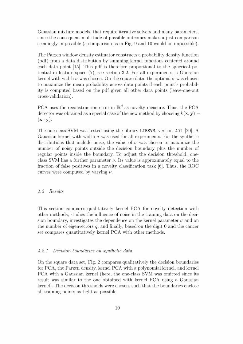
Gaussian mixture models, that require iterative solvers and many parameters,since the consequent multitude of possible outcomes makes a just comparisonseemingly impossible (a comparison as in Fig. 9 and 10 would be impossible).

The Parzen window density estimator constructs a probability density function(pdf) from a data distribution by summing kernel functions centered aroundeach data point [15]. This pdf is therefore proportional to the spherical po-tential in feature space (7), see section 3.2. For all experiments, a Gaussiankernel with width σ was chosen. On the square data, the optimal σ was chosento maximize the mean probability across data points if each point’s probabil-ity is computed based on the pdf given all other data points (leave-one-outcross-validation).

PCA uses the reconstruction error in IRd as novelty measure. Thus, the PCAdetector was obtained as a special case of the new method by choosing k(x,y) =(x · y).

The one-class SVM was tested using the library LIBSVM, version 2.71 [20]. AGaussian kernel with width σ was used for all experiments. For the syntheticdistributions that include noise, the value of σ was chosen to maximize thenumber of noisy points outside the decision boundary plus the number ofregular points inside the boundary. To adjust the decision threshold, one-class SVM has a further parameter ν. Its value is approximately equal to thefraction of false positives in a novelty classification task [6]. Thus, the ROCcurves were computed by varying ν.

4.2 Results

This section compares qualitatively kernel PCA for novelty detection withother methods, studies the influence of noise in the training data on the deci-sion boundary, investigates the dependence on the kernel parameter σ and onthe number of eigenvectors q, and finally, based on the digit 0 and the cancerset compares quantitatively kernel PCA with other methods.

4.2.1 Decision boundaries on synthetic data

On the square data set, Fig. 2 compares qualitatively the decision boundariesfor PCA, the Parzen density, kernel PCA with a polynomial kernel, and kernelPCA with a Gaussian kernel (here, the one-class SVM was omitted since itsresult was similar to the one obtained with kernel PCA using a Gaussiankernel). The decision thresholds were chosen, such that the boundaries encloseall training points as tight as possible.

10

PCA Parzen

0

0.5

1

1.5

2

2.5

3

0 0.5 1 1.5 2 2.5 3 0

0.5

1

1.5

2

2.5

3

0 0.5 1 1.5 2 2.5 3

Kernel PCA, polynom Kernel PCA, RBF

0

0.5

1

1.5

2

2.5

3

3.5

4

0 0.5 1 1.5 2 2.5 3 3.5 4

q = 1q = 5q = 9

0

0.5

1

1.5

2

2.5

3

0 0.5 1 1.5 2 2.5 3

Fig. 2. Decision boundaries for various methods: (Top left) PCA reconstruction errorwith q = 1 eigenvector, (Top right) Parzen window density estimator with σ = 0.05,(Bottom left) reconstruction error in F with polynomial kernel k(xi,xj) = (xi ·xj)

10

and various q values, (Bottom right) reconstruction error in F with Gaussian kernelusing σ = 0.4 and q = 40.

The Parzen density does not generalize well: the decision boundary followsthe irregularities of the distribution (a larger σ did not improve the boundaryeither—see Fig. 7). A linear model like PCA cannot describe the square distri-bution. Kernel PCA with a polynomial kernel does not suitably describe thisdistribution either (other polynomial degrees did not give significantly betterresults). With a Gaussian kernel, however, the decision boundary follows theshape of the distribution without getting disturbed by local irregularities. Thisability is further illustrated using the ring-line-square (Fig. 3) and the spiraldistribution (Fig. 4).

To test how the reconstruction-error boundaries cope with noise within thetraining data, the square-noise and the sine-noise distributions were used, andthe result is compared with the one-class SVM (Fig. 5 and 6). For kernel PCA,the decision threshold was chosen such that the fraction of outliers equals thegiven fraction η of noise points; for the one-class SVM, ν was set equal toη. Using the reconstruction error in F , the decision boundary can enclose

11

0

0.5

1

1.5

2

2.5

3

0 1 2 3 4 5 6 7

Fig. 3. Decision boundary for the ring-line-square distribution using the reconstruc-tion error in F with σ = 0.4 and q = 40.

0

0.5

1

1.5

2

2.5

3

0 0.5 1 1.5 2 2.5 3

Fig. 4. Decision boundary for the spiral distribution using the reconstruction errorin F with σ = 0.25 and q = 40.

smoothly the main part of the data, almost undisturbed by noise 2 ; the SVMboundary extends into the outlier region.

Kernel PCA depends on the number of principal components q and on thewidth of the Gaussian kernel σ. On the square distribution, for small σ, in-creasing the number of eigenvectors changed only little the shape of the deci-sion boundary (Fig. 7). Increasing both σ and q resulted in a good performance(Fig. 7).

4.2.2 Novelty detection on real-world data

On both the digit 0 and the cancer data set, kernel PCA for novelty detectioncould achieve lower classification errors compared with the one-class SVM,PCA, and the Parzen density (Fig. 8 to 10). Since all tested methods dependon free parameters, the area under the ROC curve is shown as a function ofthese parameters. This illustration demonstrates that for PCA, the Parzen

2 The number of principal components is lower compared with the no-noise case;otherwise, the boundary would also include nearby noise.

12

Kernel PCA

0

0.5

1

1.5

2

2.5

3

0 0.5 1 1.5 2 2.5 3

e3

e1

e2

One-class SVM

0

0.5

1

1.5

2

2.5

3

0 0.5 1 1.5 2 2.5 3

e3

e1

e2

Fig. 5. Decision boundaries on noisy data comparing kernel PCA (σ = 0.3, q = 20)with the one-class SVM (σ = 0.362, ν = 1/9). (Left) Result on the square-noise set.(Right) Illustration of the corresponding decision boundaries in F (see Figure 1).

Kernel PCA

-1.5

-1

-0.5

0

0.5

1

1.5

0 1 2 3 4 5 6

One-class SVM

-1.5

-1

-0.5

0

0.5

1

1.5

0 1 2 3 4 5 6

Fig. 6. Decision boundaries for the sine-noise distribution comparing kernel PCA(σ = 0.4, q = 40) with the one-class SVM (σ = 0.489, ν = 2/7).

13

σ

0

0.5

1

1.5

2

2.5

3

0 0.5 1 1.5 2 2.5 3 0

0.5

1

1.5

2

2.5

3

0 0.5 1 1.5 2 2.5 3

0

0.5

1

1.5

2

2.5

3

0 0.5 1 1.5 2 2.5 3 0

0.5

1

1.5

2

2.5

3

0 0.5 1 1.5 2 2.5 3

0

0.5

1

1.5

2

2.5

3

0 0.5 1 1.5 2 2.5 3 0

0.5

1

1.5

2

2.5

3

0 0.5 1 1.5 2 2.5 3

q

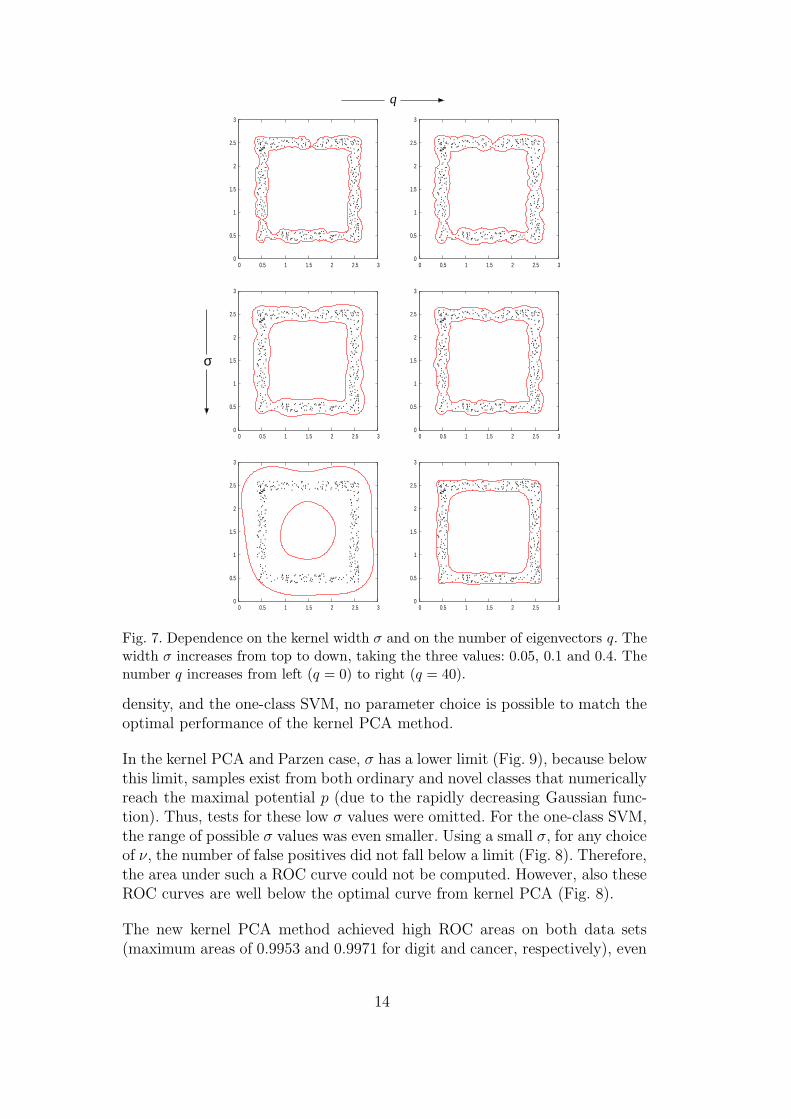
Fig. 7. Dependence on the kernel width σ and on the number of eigenvectors q. Thewidth σ increases from top to down, taking the three values: 0.05, 0.1 and 0.4. Thenumber q increases from left (q = 0) to right (q = 40).

density, and the one-class SVM, no parameter choice is possible to match theoptimal performance of the kernel PCA method.

In the kernel PCA and Parzen case, σ has a lower limit (Fig. 9), because belowthis limit, samples exist from both ordinary and novel classes that numericallyreach the maximal potential p (due to the rapidly decreasing Gaussian func-tion). Thus, tests for these low σ values were omitted. For the one-class SVM,the range of possible σ values was even smaller. Using a small σ, for any choiceof ν, the number of false positives did not fall below a limit (Fig. 8). Therefore,the area under such a ROC curve could not be computed. However, also theseROC curves are well below the optimal curve from kernel PCA (Fig. 8).

The new kernel PCA method achieved high ROC areas on both data sets(maximum areas of 0.9953 and 0.9971 for digit and cancer, respectively), even

14

Digit 0 Cancer

0

0.2

0.4

0.6

0.8

1

0 0.2 0.4 0.6 0.8 1

KPCA1-class SVM, σ = 1.21-class SVM, σ = 2 1-class SVM, σ = 10

0.8

0.82

0.84

0.86

0.88

0.9

0.92

0.94

0.96

0.98

1

0 0.05 0.1 0.15 0.2

true

pos

itive

s

false positives

0

0.2

0.4

0.6

0.8

1

0 0.2 0.4 0.6 0.8 1

KPCA1-class SVM, σ = 11-class SVM, σ = 10

0.8

0.82

0.84

0.86

0.88

0.9

0.92

0.94

0.96

0.98

1

0 0.05 0.1 0.15 0.2

true

pos

itive

s

false positives

Fig. 8. ROC curves on the digit and the cancer data. Kernel PCA using σ = 4 andq = 100 (digit 0) and σ = 2 and q = 190 (cancer) is compared with the one-classSVM for various σ values.

Digit 0 Cancer

σkernel width

0.955

0.96

0.965

0.97

0.975

0.98

0.985

0.99

0.995

1

0.1 1 10 100

q = 200q = 10

Parzen1-class SVM

area

und

er R

OC

cur

ve

σkernel width

0.9958

0.996

0.9962

0.9964

0.9966

0.9968

0.997

0.9972

0.1 1 10

q = 190q = 100Parzen

area

und

er R

OC

cur

ve

Fig. 9. Performance depending on the kernel width σ using the digit and the cancerdata. Kernel PCA for various q values is compared with the Parzen density and theone-class SVM. For the cancer data, the ROC area of the one-class SVM is belowthe range shown in this diagram.

though, the structure of the data appears to be different in both cases. Onthe digit set, a linear model like PCA does better than the Parzen density(maximum area: 0.9893 versus 0.9873); on the cancer set, however, the Parzendensity does very good (maximum area: 0.9966), but PCA does much worse(maximum area: 0.9828).

Furthermore, the results show the behavior in the limit of small and large σvalues. For small σ, the performance of the reconstruction error in F and ofthe Parzen density become almost equal (Fig. 9). This behavior matches the

15

Digit 0 Cancer

qnum. of eigenvectors

0.9

0.91

0.92

0.93

0.94

0.95

0.96

0.97

0.98

0.99

1

0 20 40 60 80 100

σ = 4σ = 50σ = 100

PCA

area

und

er R

OC

cur

ve

qnum. of eigenvectors

0.975

0.98

0.985

0.99

0.995

1

0 10 20 30 40 50 60 70 80

σ = 1σ = 5σ = 15

PCA

area

und

er R

OC

cur

veFig. 10. Performance depending on the number of eigenvectors q using the digit andthe cancer data. Kernel PCA for various σ values is compared with standard PCA.

observation of the decision boundaries (Fig. 7). For large σ, the performancereaches the level of PCA, if q is smaller than d—otherwise PCA is meaningless(Fig. 10). This limit behavior can be also predicted theoretically (see appendixA).

A final test further illustrates the proper function of the new method. Thereconstruction error in F was used to find unusual ‘0’ digits within in theMNIST test set. Fig. 11 displays the ten digits that had the highest recon-struction errors. Most of these samples look indeed unusual.

p = 0.033 p = 0.032 p = 0.031 p = 0.023

p = 0.021 p = 0.021 p = 0.019 p = 0.019 p = 0.018

p = 0.036

Fig. 11. The 10 most unusual ‘0’ digits from the MNIST test set. The digits arearranged in descending order of their reconstruction error p (σ = 4, q = 100). Thefigure shows the unprocessed digits of size 28 × 28 pixels; for novelty detection,however, the processed digits (8 × 8 pixels) were used.

16

5 Discussion

This section discusses the effect of noise in the training data, mentions concernsabout the computational complexity of the new method, and points out otherrelated methods.

5.1 Noisy data

Novelty detectors learn from data that are assumed to contain only represen-tatives of the ordinary class. In real applications, however, these data containnoise, thus, outliers. Therefore, a good novelty detector should be robust tonoise. In the presented model, outliers might distort the principal componentsextracted by kernel PCA. Like PCA, its kernel variant is not robust againstsuch noise [21,22]. However, as for PCA, also for kernel PCA, robust ver-sions exist [21,22]. These approaches essentially try to remove outliers, eitherbefore or in alternation with computing the principal components. The pre-sented method has the advantage that it uses a standard algorithm, kernelPCA. Thus, improvements and modifications of this algorithm can be readilyapplied.

No robust versions of kernel PCA were used here for the reported experi-ments; nevertheless, the new decision boundaries appeared to be robust undernoise (Fig. 5 and 6). This robustness may be explained by the almost uni-form variance of the added noise; thus, probably, the principal componentswere undisturbed. This noise, however, did disturb the results of the one-classSVM (Fig. 5 and 6). In feature space, the sphere (the SVM boundary on S)that encloses the data is less tight around the noise-free part of the distribu-tion than the reconstruction-error boundary (section 3.1). Thus, for the samenumber of enclosed points, the one-class SVM encloses more outliers than thenew method (Fig. 5, Right).

5.2 Computational complexity

Kernel PCA is computational expensive. Most time consuming is the extrac-tion of the eigenvectors of K, which is O(n3) if extracting all eigenvectors[23]. Additionally, if searching for the parameters σ and q, for example, bycross-validation, the computation time is further multiplied by the number ofPCA evaluations. Kernel PCA is also memory exhaustive: the n × n matrixK needs to be stored, and in the presented experiments, only a tiny fractionof entries in K were almost zero. Therefore, on large data sets, Monte-Carlosampling is necessary.

17

Furthermore, testing is expensive. For each new data point, the kernel functionneeds to be evaluated n-times. However, this number could be reduced usingso-called ‘reduced-set methods’ [24,25].

The one-class SVM is faster: using an Athlon 1800+, on the digit-0 data,with σ = 2 and ν = 0.1, LIBSVM needed 1.3 seconds for training and 0.5seconds to classify all test patterns. In contrast, kernel PCA with σ = 4 andq = 100 needed 31.6 seconds for training (computing the kernel matrix andextracting eigenvectors) and 34.4 seconds for testing. However, computing aROC curve using the reconstruction error does not require any noticeableadditional computation time, but the one-class SVM needs to be retrained fordifferent ν values.

5.3 Related methods

The reconstruction error in F is similar to but differs from the squared errorin the denoising application of kernel PCA [26]. To denoise a pattern x, itsmapping Φ(x) is projected onto the principal subspace. The denoised pat-tern z is obtained by minimizing the squared distance between Φ(z) and theprojection of Φ(x). Figure 12 illustrates the difference to the reconstructionerror.

(z)

Φ

Φ

(x)

principal component

denoising distancep

Fig. 12. The difference between the distance to be optimized in denoising and thereconstruction error p.

Tax and Juszczak [9] used kernel PCA as a preprocessing step for noveltydetection. Kernel PCA is used to whiten (to make the variance in each di-rection equal) the data in feature space. Later, these data are enclosed by asphere to obtain a one-class classifier [8]. A problem for whitening are direc-tions with variance close to zero. In the present study, the variance is close tozero for most directions a distribution expands to (if σ is not too small). Thus,whitening is disadvantageous because on the one hand, normalizing these di-rections is prone to computational errors, and on the other hand, omittingthese directions ignores the low variance, since everything will be enclosed ina sphere.

18

6 Conclusions

This article studied kernel PCA for novelty detection. A principal subspacein an infinite-dimensional feature space described the distribution of trainingdata. The reconstruction error of a new data point with respect to this sub-space was used as a measure for novelty. This new method demonstrated ahigher ordinary/novel-classification performance on a handwritten-digit anda breast-cancer database compared with the one-class SVM and the Parzenwindow density estimator. Both of these methods were competitive in pastexperiments [1,2].

Using the reconstruction error in feature space, the decision boundaries fol-lowed smoothly the shape of two-dimensional synthetic distributions, withoutgetting distorted by the position of single data points. Thus, the new methodappears to generalize better compared with the Parzen density. Furthermore,compared with the one-class SVM, the presented method demonstrated to bemore robust against noise within the training set.

This article demonstrated the dependence on the kernel parameter σ andon the number of eigenvectors q. For small σ, the new method behaved likethe Parzen density. For large σ, the reconstruction error in feature space ap-proaches the reconstruction error for standard PCA. The number of eigen-vectors q had to be sufficiently large for a near optimal performance on bothreal-world data sets and on the synthetic distributions without noise.

Future work aims at finding rules for choosing the two free parameters, σ andq (without the need of a time-consuming cross-validation step). Of advantageshould be therein that a wide range of parameters resulted in a near opti-mal performance. Furthermore, the range of usable data distributions needsto be explored. The arguments in section 3.1 already suggest that such distri-butions have to originate from an underlying manifold or from some locallyconnected structure, as also most dimension-reduction techniques require (see,for example, mixture of local PCA [27] and locally linear embedding [28]).

7 Acknowledgments

I thank the anonymous reviewers, whose comments helped to improve themanuscript.

19

A Behavior at large kernel widths

This section analyzes theoretically the behavior of the reconstruction error infeature space at large widths σ of the Gaussian kernel. For σ ≫ max ||xi−xj ||and q < d, the ‘kernelized’ reconstruction error approaches the reconstructionerror in the original space IRd.

We assume σ ≫ max ||xi−xj ||, and thus, ignore orders smaller than O(1/σ2).Therefore, the Gaussian kernel can be approximated as k(x,y) ≈ 1 − ||x −y||2/(2σ2). We will show that with this approximation, the reconstructionerror (11) is proportional to (11) with k(x,y) = (x · y), which corresponds tostandard PCA. First, substituting the approximated kernel into the spherical-potential component (6) gives

pS(z) ≈ 1

σ2

(z · z) − 2

n

∑

i

(z · xi) +1

n2

∑

i,j

(xi · xj)

. (A.1)

This potential pS has two important properties: it scales as 1/σ2, and theexpression in the square brackets equals the spherical-potential componentfor the polynomial kernel k(x,y) = (x · y).

In addition, we use the above substitution to compute the eigenvector projec-tions (9):

fl(z) ≈ 1

σ2

∑

i

αli

(z · xi) −1

n

∑

r

(xi · xr)

− 1

n

∑

r

(z · xr) +1

n2

∑

r,s

(xr · xs)

. (A.2)

Again, the expression in the square brackets is the same as for k(x,y) = (x·y).We still need to evaluate how αl

i depends on the approximated kernel function.The variables αl

i are the components of the eigenvectors of the kernel matrixK, which is computed according to (4) such that the data have zero mean infeature space (see section 2). Substituting the approximated kernel functioninto (4) gives

Kij ≈1

σ2

(xi · xj) −1

n

∑

r

(xi · xr)

− 1

n

∑

r

(xj · xr) +1

n2

∑

r,s

(xr · xs)

. (A.3)

20

Apart from the factor 1/σ2, this formula is the same as for k(x,y) = (x · y).Thus, in both cases, also the eigenvectors are the same, but the eigenvaluesdiffer by the factor 1/σ2. Since the length of α is 1/

√λ (see section 2), the

components αli for the approximated Gaussian kernel equal the corresponding

components for PCA times σ. Thus, since fl is squared in (11), we again havethe same 1/σ2 factor as in (A.1). In total, the reconstruction error in featurespace differs only by a constant factor from the reconstruction error in theoriginal space. Therefore, the results on novelty detection are the same.

References

[1] M. Markou, S. Singh, Novelty detection: A review, part 1: Statisticalapproaches, Signal Processing 83 (12) (2003) 2481–2497.

[2] M. Markou, S. Singh, Novelty detection: A review, part 2: Neural network basedapproaches, Signal Processing 83 (12) (2003) 2499–2521.

[3] L. Tarassenko, P. Hayton, N. Cerneaz, M. Brady, Novelty detection for theidentification of masses in mammograms, in: Proceedings of the 4th IEEInternational Conference on Artificial Neural Networks, IEE, 1995, pp. 442–447.

[4] H. Cheng, X. Shi, R. Min, L. Hu, X. Cai, H. Du, Approaches for automateddetection and classification of masses in mammograms, Pattern Recognition39 (4) (2006) 646–668.

[5] B. Scholkopf, A. J. Smola, Learning with Kernels, MIT Press, Cambridge, MA,2002.

[6] B. Scholkopf, R. C. Williamson, A. J. Smola, J. Shawe-Taylor, J. Platt, Supportvector method for novelty detection, Advances in Neural Information ProcessingSystems 12 (2000) 582–588.

[7] B. Scholkopf, J. C. Platt, J. Shawe-Taylor, A. J. Smola, R. C. Williamson,Estimating the support of a high-dimensional distribution, Neural Computation13.

[8] D. M. J. Tax, R. P. W. Duin, Support vector domain description, PatternRecognition Letters 20 (1999) 1191–1199.

[9] D. M. J. Tax, P. Juszczak, Kernel whitening for one-class classification, LectureNotes in Computer Science 2388 (2002) 40–52.

[10] L. Tarassenko, A. Nairac, N. Townsend, P. Cowley, Novelty detection in jetengines, in: IEE Colloquium on Condition Monitoring: Machinery, ExternalStructures and Health (Ref. No. 1999/034), IEE, 1999, pp. 4/1 – 4/5.

21

[11] S. O. Song, D. Shin, E. S. Yoon, Analysis of novelty detection properties ofautoassociators, in: A. G. Starr, R. B. K. N. Rao (Eds.), Proceedings of the 14thInternational Congress and Exhibition on Condition Monitoring and DiagnosticEngineering Management (COMADEM), Elsevier Science, 2001, pp. 577–584.

[12] B. Scholkopf, A. J. Smola, K.-R. Muller, Nonlinear component analysis as akernel eigenvalue problem, Neural Computation 10 (1998) 1299–1319.

[13] A. Wald, Statistical Decision Functions, Wiley, New York, 1950.

[14] L. Lusted, Introduction to Medical Decision Making, Thomas, Springfield, IL,1968.

[15] E. Parzen, On estimation of a probability density function and mode, Annalsof Mathematical Statistics 33 (1962) 1065–1076.

[16] K. I. Diamantaras, S. Y. Kung, Principal Component Neural Networks, JohnWiley & Sons, New York, 1996.

[17] Y. LeCun, The MNIST database of handwritten digits [http://yann.lecun.com/exdb/mnist/] (1998).

[18] C. Blake, C. Merz, UCI repository of machine learning databases[http://www.ics.uci.edu/∼mlearn/MLRepository.html] (1998).

[19] W. H. Wolberg, O. L. Mangasarian, Multisurface method of pattern separationfor medical diagnosis applied to breast cytology, Proceedings of the NationalAcademy of Sciences of the USA 87 (1990) 9193–9196.

[20] C.-C. Chang, C.-J. Lin, LIBSVM: A library for support vector machines[http://www.csie.ntu.edu.tw/∼cjlin/libsvm] (2001).

[21] T. Takahashi, T. Kurita, Robust de-noising by kernel PCA, in: Proceedings ofthe International Conference on Artificial Neural Networks, Vol. LNCS 2415,Springer, 2002, pp. 739–744.

[22] C.-D. Lu, T.-Y. Zhang, X.-Z. Du, C.-P. Li, A robust kernel PCA algorithm,in: Proceedings of the International Conference on Machine Learning andCybernetics, Vol. 5, IEEE, 2004, pp. 3084–3087.

[23] W. H. Press, S. A. Teukolsky, W. T. Vetterling, B. P. Flannery, NumericalRecipes in C: The Art of Scientific Computing, Cambridge University Press,UK, 1993.

[24] C. J. C. Burges, Simplified support vector decision rules, in: L. Saitta (Ed.),Proceedings of the 13th International Conference on Machine Learning, MorganKaufmann, San Mateo, CA, 1996, pp. 71–77.

[25] B. Scholkopf, P. Knirsch, A. J. Smola, C. Burges, Fast approximation of supportvector kernel expansions, and an interpretation of clustering as approximationin feature spaces, in: P. Levi, R.-J. Ahlers, F. May, M. Schanz (Eds.), 20. DAGMSymposium Mustererkennung, Springer, Berlin, 1998, pp. 124–132.

22

[26] S. Mika, B. Scholkopf, A. J. Smola, K.-R. Muller, M. Scholz, G. Ratsch,Kernel PCA and de-noising in feature spaces, Advances in Neural InformationProcessing Systems 11 (1999) 536–542.

[27] M. E. Tipping, C. M. Bishop, Mixtures of probabilistic principal componentanalyzers, Neural Computation 11 (1999) 443–482.

[28] S. T. Roweis, L. K. Saul, Nonlinear dimensionality reduction by locally linearembedding, Science 290 (2000) 2323–2326.

23