Kernel-Induced Feature Spaces - University of Iceland · Kernel-Induced Feature Spaces Chapter3...

Kernel-Induced Feature Spaces

Chapter 3

March 6, 2003

T.P. Runarsson ([email protected]) and S. Sigurdsson ([email protected])

March 6, 2003

Kernel representation

• Complex real-world applications require more expressive

hypothesis spaces than linear functions (ie. cannot be

expressed as a simple linear combinations of input attributes).

• This limitation was pointed out by Minsky and Papert in the1960s and led to the proposal of multi layered neural networks.

• Kernel representations offer an alternative solution by

projecting the input attributes into a high dimensional feature

space, thus increasing the computational power of the linear

learning machines discussed so far.

• The kernel method allows the decoupling of the learningalgorithm and theory from the design of an appropriate kernel

for a specific application area.

1

March 6, 2003

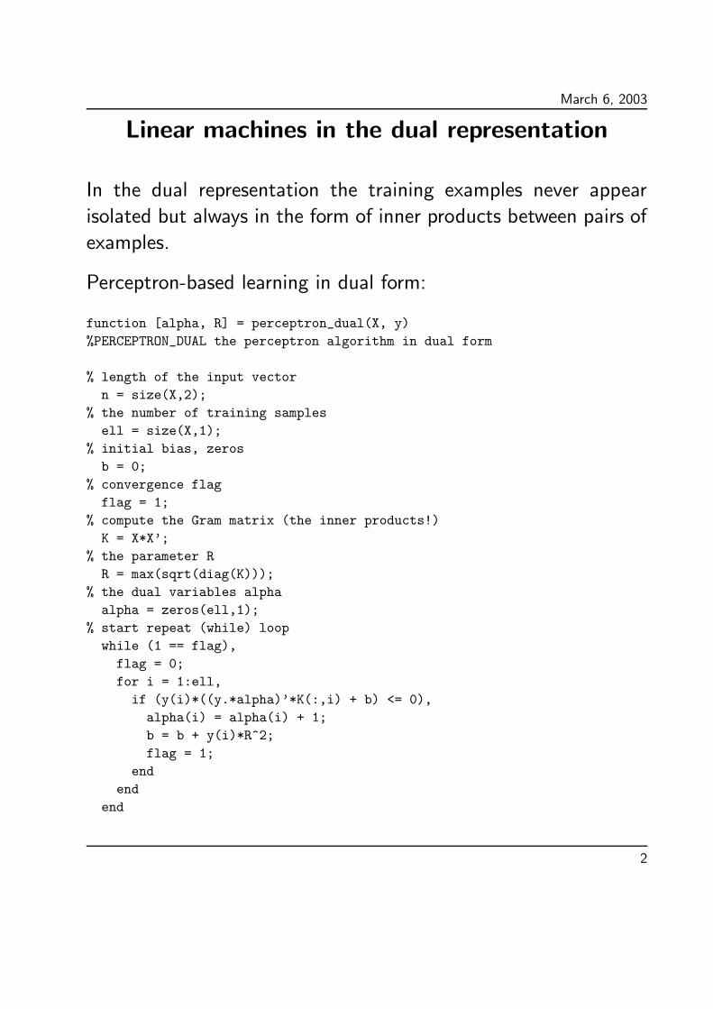
Linear machines in the dual representation

In the dual representation the training examples never appear

isolated but always in the form of inner products between pairs of

examples.

Perceptron-based learning in dual form:

function [alpha, R] = perceptron_dual(X, y)

%PERCEPTRON_DUAL the perceptron algorithm in dual form

% length of the input vector

n = size(X,2);

% the number of training samples

ell = size(X,1);

% initial bias, zeros

b = 0;

% convergence flag

flag = 1;

% compute the Gram matrix (the inner products!)

K = X*X’;

% the parameter R

R = max(sqrt(diag(K)));

% the dual variables alpha

alpha = zeros(ell,1);

% start repeat (while) loop

while (1 == flag),

flag = 0;

for i = 1:ell,

if (y(i)*((y.*alpha)’*K(:,i) + b) <= 0),

alpha(i) = alpha(i) + 1;

b = b + y(i)*R^2;

flag = 1;

end

end

end

2

March 6, 2003

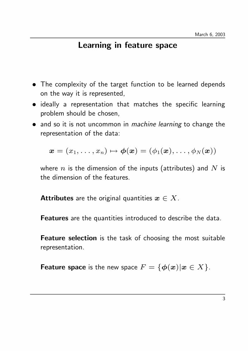
Learning in feature space

• The complexity of the target function to be learned dependson the way it is represented,

• ideally a representation that matches the specific learningproblem should be chosen,

• and so it is not uncommon in machine learning to change therepresentation of the data:

x = (x1, . . . , xn) 7→ φ(x) = (φ1(x), . . . , φN(x))

where n is the dimension of the inputs (attributes) and N is

the dimension of the features.

Attributes are the original quantities x ∈ X.

Features are the quantities introduced to describe the data.

Feature selection is the task of choosing the most suitable

representation.

Feature space is the new space F = {φ(x)|x ∈ X}.

3

March 6, 2003

Feature selection

Motivation:

• To improve generalization error,• for explanatory purposes determine the relevant features,• and reduce the dimensionality of the input space (for real-timeapplications).

Good feature selection requires domain knowledge (“insight”), for

example what would be a good feature for say:

• a pixel image,• text document,• a living creature,• the stock market,• some physical phenomenon (Newton’s law of gravity),• . . . ?

4

March 6, 2003

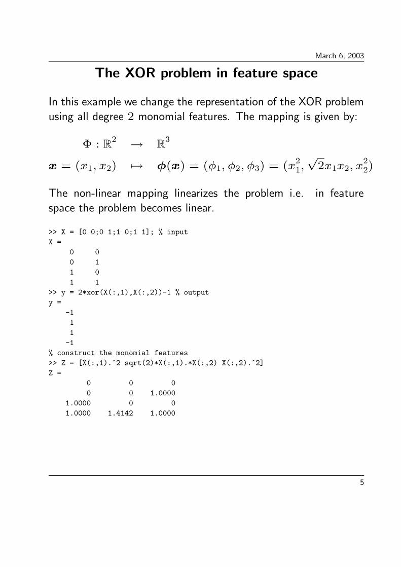
The XOR problem in feature space

In this example we change the representation of the XOR problem

using all degree 2 monomial features. The mapping is given by:

Φ : R2 → R3

x = (x1, x2) 7→ φ(x) = (φ1, φ2, φ3) = (x21,√2x1x2, x

22)

The non-linear mapping linearizes the problem i.e. in feature

space the problem becomes linear.

>> X = [0 0;0 1;1 0;1 1]; % input

X =

0 0

0 1

1 0

1 1

>> y = 2*xor(X(:,1),X(:,2))-1 % output

y =

-1

1

1

-1

% construct the monomial features

>> Z = [X(:,1).^2 sqrt(2)*X(:,1).*X(:,2) X(:,2).^2]

Z =

0 0 0

0 0 1.0000

1.0000 0 0

1.0000 1.4142 1.0000

5

March 6, 2003

% let’s just use the above perceptron algorithm

>> [alpha, R] = perceptron_dual(Z,y)

alpha =

17

11

11

6

R =

2

>> b = alpha’*(y*R^2)

b =

-4

>> w = (alpha.*y)’*Z

w =

5.0000 -8.4853 5.0000

% note that the problem is 3-dimensional

>> w*Z’+b

ans =

-4.0000 1.0000 1.0000 -6.0000

>> sign(w*Z’+b)

ans =

-1 1 1 -1

6

March 6, 2003

The separating hyperplane in feature space

−0.50

0.51

−0.50

0.51

−0.5

0

0.5

1

φ1φ

2

φ 3

The plane (w, b) = ((5,−8.4853, 5),−2) separating the XORtask linearly in feature space.

7

March 6, 2003

The implicit mapping into feature space

Consider the monomial features mapping:

Φ : Rn → RN

For different monomials of degree d the dimension of the feature

space is:(d+ n− 1

d

)

=(d+ n− 1)!

d!(n− 1)!and so it becomes very quickly intractable to work directly in

feature space.

There exists, however, a way of computing dot products in these

high-dimensional feature spaces without explicitly mapping into

the spaces. This is done by means of kernels nonlinear in the

input space X.

A kernel is a function K, such that for all x, z ∈ X

K(x, z) =⟨

φ(x) · φ(z)⟩

where φ is a mapping fromX to an (inner product) feature space

F .

8

March 6, 2003

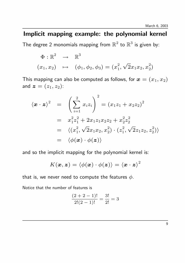
Implicit mapping example: the polynomial kernel

The degree 2 monomials mapping from R2 to R3 is given by:

Φ : R2 → R3

(x1, x2) 7→ (φ1, φ2, φ3) = (x21,√2x1x2, x

22)

This mapping can also be computed as follows, for x = (x1, x2)

and z = (z1, z2):

〈x · z〉2 =

(

2∑

i=1

xizi

)2

= (x1z1 + x2z2)2

= x21z

21 + 2x1z1x2z2 + x

22z

22

= 〈(x21,√2x1x2, x

22) · (z

21,√2z1z2, z

22)〉

= 〈φ(x) · φ(z)〉

and so the implicit mapping for the polynomial kernel is:

K(x, z) = 〈φ(x) · φ(z)〉 = 〈x · z〉2

that is, we never need to compute the features φ.

Notice that the number of features is

(2 + 2− 1)!

2!(2− 1)!=

3!

2!= 3

9

March 6, 2003

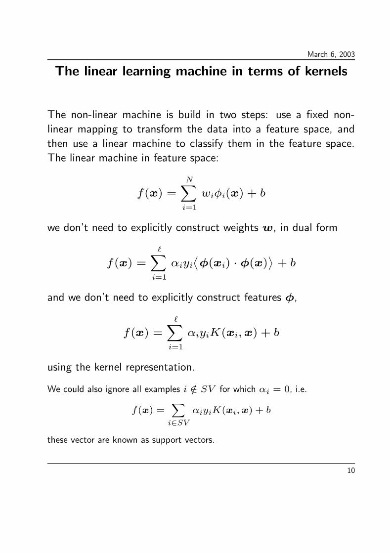
The linear learning machine in terms of kernels

The non-linear machine is build in two steps: use a fixed non-

linear mapping to transform the data into a feature space, and

then use a linear machine to classify them in the feature space.

The linear machine in feature space:

f(x) =

N∑

i=1

wiφi(x) + b

we don’t need to explicitly construct weights w, in dual form

f(x) =∑

i=1

αiyi⟨

φ(xi) · φ(x)⟩

+ b

and we don’t need to explicitly construct features φ,

f(x) =∑

i=1

αiyiK(xi,x) + b

using the kernel representation.

We could also ignore all examples i /∈ SV for which αi = 0, i.e.

f(x) =∑

i∈SVαiyiK(xi,x) + b

these vector are known as support vectors.

10

March 6, 2003

The perceptron using a kernel?

Our perceptron algorithm in dual form with only one small change:

function [alpha, R] = perceptron_dual_poly(X, y, d)

%PERCEPTRON_DUAL_POLY perceptron algorithm in dual form + polynomial kernel

% length of the input vector

n = size(X,2);

% the number of training samples

ell = size(X,1);

% initial bias, zeros

b = 0;

% convergence flag

flag = 1;

% compute the *Kernel* matrix

K = (X*X’).^d; % <----

% the parameter R

R = max(sqrt(diag(K)));

% the dual variables alpha

alpha = zeros(ell,1);

% start repeat (while) loop

while (1 == flag),

flag = 0;

for i = 1:ell,

if (y(i)*((y.*alpha)’*K(:,i) + b) <= 0),

alpha(i) = alpha(i) + 1;

b = b + y(i)*R^2;

flag = 1;

end

end

end

11

March 6, 2003

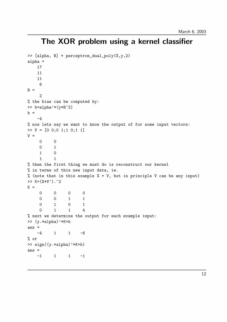
The XOR problem using a kernel classifier

>> [alpha, R] = perceptron_dual_poly(X,y,2)

alpha =

17

11

11

6

R =

2

% the bias can be computed by:

>> b=alpha’*(y*R^2)

b =

-4

% now lets say we want to know the output of for some input vectors:

>> V = [0 0;0 1;1 0;1 1]

V =

0 0

0 1

1 0

1 1

% then the first thing we must do is reconstruct our kernel

% in terms of this new input data, ie.

% (note that in this example X = V, but in principle V can be any input)

>> K=(X*V’).^2

K =

0 0 0 0

0 0 1 1

0 1 0 1

0 1 1 4

% next we determine the output for each example input:

>> (y.*alpha)’*K+b

ans =

-4 1 1 -6

% or

>> sign((y.*alpha)’*K+b)

ans =

-1 1 1 -1

12

March 6, 2003

Optical character recognition demo

We experiment with the US Postal Service OCR database which

contains 7291 examples for the purpose of training and 2007

examples for testing. The object is to learn to recognize 16× 16

pixel images of handwritten digits from 0 to 9. For example, here

are the characters 6, 2, 6, 5, 5, 8 and 2:6(4,2,0) 2(3,2,0) 6(2,4,5) 5(2,5,3) 5(8,5,2) 8(4,8,0) 2(0,3,2) 4(9,4,1) 6(4,6,8) 8(3,8,4)

5(4,5,0) 6(2,4,0) 9(7,9,2) 2(0,2,5) 8(3,8,4) 0(9,8,7) 6(5,2,4) 6(4,3,2) 8(3,2,0) 1(4,1,7)

8(3,5,2) 1(6,2,1) 5(8,5,9) 8(2,8,3) 9(2,7,8) 8(0,8,3) 2(3,8,0) 9(5,7,3) 9(7,4,5) 5(3,5,2)

5(3,5,6) 7(4,0,3) 1(7,1,9) 8(2,7,4) 3(5,3,8) 1(6,2,5) 8(0,5,8) 9(1,9,3) 7(9,3,7) 0(4,0,5)

3(8,4,5) 0(2,0,4) 0(4,0,5) 2(8,2,9) 2(8,2,3) 2(8,2,3) 2(3,0,8) 8(3,5,2) 0(2,0,3) 8(3,2,8)

The kernel based dual perceptron algorithm was tested on this

data in a similar way to the XOR problem. However, this

is a multi-classification problem and so 10 one-against-the-rest

perceptrons are trained.

To run this demo you will need the data files:

usps digits training.mat and usps digits testing.mat.

Also the MATLAB script ocrdemo.m and the MATLAB functions

perceptron dual kernel.m and the kernel function kernel.m.

Because of memory limitations in MATLAB only the first≈ 2000

examples of the 7291 are used for training. In this case we get a

classification error of 8.37%.

13

March 6, 2003

The OCR demo using pairwise classification

In pairwise classification, er train a classifier for each possible

pair of classes. For m classes, this results in (m − 1)m/2

binary classifiers. This values is larger than the one-against-the

rest classifiers, which are 10 in this demo, but 45 using pairwise

classification.

At first this may seem to be a slower approach, but actually the

training sets are smaller and so it is actually possible to save

time! Furthermore, because the training sets are smaller it was

now possible to use the entire training set in MATLAB.

We ran 45 binary classifiers on the whole data set and used a

voting scheme for classification, i.e. the class which gets the

highest number of votes wins! in this case a classification error of

6.38% was achived (probably because we used the whole training

set).

The problem with the one-against-the-rest is that the real valued

ouputs are on different scales! However, this is the most common

approach today and some efforts are being made in tranforming

the real valued ouputs into class probabilities.

14

March 6, 2003

Features for strings and texts

Let Σ∗ denote the set of all strings of finite length that are madeup from characters in the set Σ. If eg. Σ = {a,b,c} thenΣ∗ = {ε, a,b,c,aa,ab,ba,bb,aaa,aab, . . .} where ε denotesthe empty string.

If s ∈ Σ∗ then |s| denotes the length of s, i.e. the number ofcharacters in s. |ε| = 0.

If u ∈ Σ∗ and s ∈ Σ∗ we say that u is a substring of s if

there exist indicies i = (i1, i2, . . . , i|u|) with 1 ≤ i1 < i2 <

. . . < i|u| ≤ |s| such that uj = sij for j = 1, . . . , |u|.Then we also write u = s(i). s[i : j] denotes the substring

si, si+1 . . . sj−1sj of length j − i+ 1.

Let m = |Σ| be the number of (distinct) characters in Σ. Thenfor a given n ≥ 1 we can define a feature map φn : Σ∗ 7→ Rmn

that associates with each string s ∈ Σ∗ a real valued vectorof length mn that contains, for every possible distinct substring

of length n, how many different such substrings there are in s.

Below we show such feature vectors for the strings s = abcaaab

and t = bcaac when n = 1, 2, 3 and Σ = {a,b,c}.

15

March 6, 2003

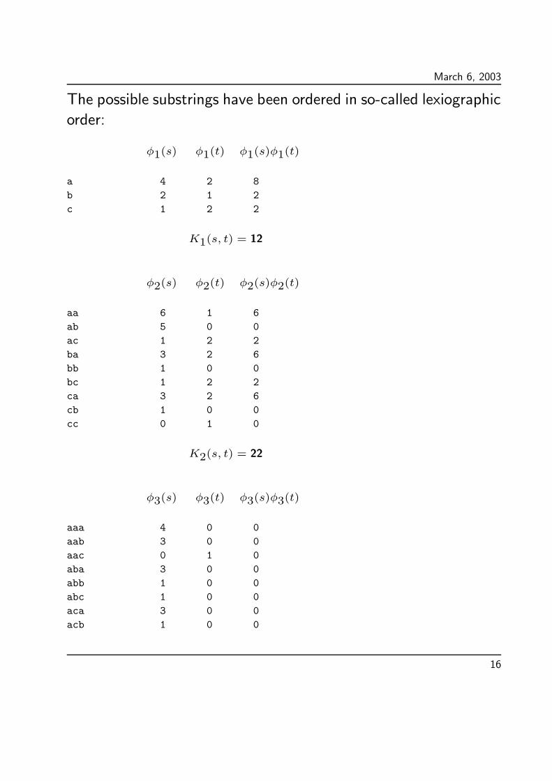
The possible substrings have been ordered in so-called lexiographic

order:

φ1(s) φ1(t) φ1(s)φ1(t)

a 4 2 8

b 2 1 2

c 1 2 2

K1(s, t) = 12

φ2(s) φ2(t) φ2(s)φ2(t)

aa 6 1 6

ab 5 0 0

ac 1 2 2

ba 3 2 6

bb 1 0 0

bc 1 2 2

ca 3 2 6

cb 1 0 0

cc 0 1 0

K2(s, t) = 22

φ3(s) φ3(t) φ3(s)φ3(t)

aaa 4 0 0

aab 3 0 0

aac 0 1 0

aba 3 0 0

abb 1 0 0

abc 1 0 0

aca 3 0 0

acb 1 0 0

16

March 6, 2003

acc 0 0 0

baa 3 1 3

bab 3 0 0

bac 0 2 0

bba 0 0 0

bbb 0 0 0

bbc 0 0 0

bca 3 2 6

bcb 1 0 0

bcc 0 1 0

caa 3 1 3

cab 3 0 0

cac 0 2 0

cba 0 0 0

cbb 0 0 0

cbc 0 0 0

cca 0 0 0

ccb 0 0 0

ccc 0 0 0

K3(s, t) = 12

17

March 6, 2003

The kernel from string features

Let Kn(s, t) denote the inner product⟨

φn(s) · φn(t)⟩

. We

now observe that Kn(s, t) can be evaluated recursively without

first explicitly constructing φn(s) and φn(t) by making use of

the following relations:

• Ko(s, t) = 1 for all s, t,

• Ki(s, t) = 0 if min(|s|, |t|) < i, i = 1, 2, . . ., and

• Ki(sx, t) = Ki(s, t) +∑

j:tj=xKi−1(s, t[1 : j − 1]),

x ∈ Σ, i = 1, 2, . . .

The last sum is the sum of allKi−1(s, t[1 : j−1]) values where

tj is the same character as x.

18

March 6, 2003

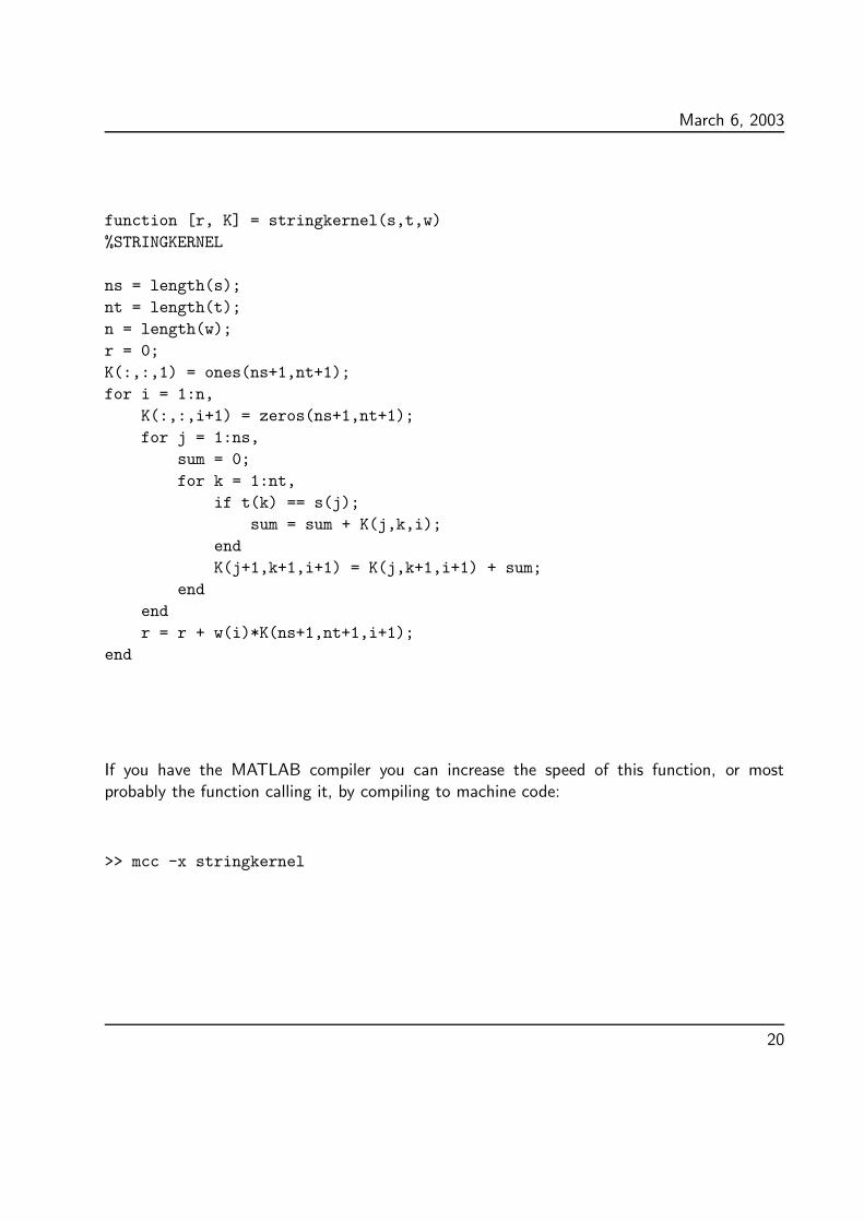
MATLAB function for the string kernel

The following MATLAB function calculates for given input strings

Kn(s, t) in a non-recursive manner by successively calculating

K0(s, t), K1(s, t), . . . , Kn(s, t).

For each fixed i we calculate successively Ki(s[1 : j], t[1 : k])

k = 0, 1, . . . |t|, j = 0, 1, . . . , |s| making use of the relationsabove. Since the indicies in MATLAB start with 1 (not 0)

Ki(s[1 : j], t[1 : k]) is denoted by K(j + 1, k + 1, i + 1).

Also note that strings in MATLAB are effectively handled as

vectors of unicode-values corresponding to the characters in the

string.

The MATLAB function is in fact more general in that it evaluates

for an input weight-vector w of length n the weighted kernel∑n

i=1wiKi(s, t).

Also note that the complexity of the algorithm is O(n|s||t|).By comparison the number of elements in the feature vector is

mn, leaving apart the number of steps required to calculate each

element.

19

March 6, 2003

function [r, K] = stringkernel(s,t,w)

%STRINGKERNEL

ns = length(s);

nt = length(t);

n = length(w);

r = 0;

K(:,:,1) = ones(ns+1,nt+1);

for i = 1:n,

K(:,:,i+1) = zeros(ns+1,nt+1);

for j = 1:ns,

sum = 0;

for k = 1:nt,

if t(k) == s(j);

sum = sum + K(j,k,i);

end

K(j+1,k+1,i+1) = K(j,k+1,i+1) + sum;

end

end

r = r + w(i)*K(ns+1,nt+1,i+1);

end

If you have the MATLAB compiler you can increase the speed of this function, or mostprobably the function calling it, by compiling to machine code:

>> mcc -x stringkernel

20

March 6, 2003

Example using the MATLAB function

Below we show the matrices Ki(s, t) when s = abcaaab,t = bcaac and i = 0, 1, 2, 3.

>> r = stringkernel(’abcaaab’,’bcaac’,[1 1 1])

r =

46

>> [r,K]=stringkernel(’abcaaab’,’bcaac’,0.9.^(2*[1:3]))

r =

30.5315

K(:,:,1) =

empty b bc bca bcaa bcaac

empty 1 1 1 1 1 1

a 1 1 1 1 1 1

ab 1 1 1 1 1 1

abc 1 1 1 1 1 1

abca 1 1 1 1 1 1

abcaa 1 1 1 1 1 1

abcaaa 1 1 1 1 1 1

abcaaab 1 1 1 1 1 1

K(:,:,2) =

0 0 0 0 0 0

0 0 0 1 2 2

0 1 1 2 3 3

0 1 2 3 4 5

0 1 2 4 6 7

0 1 2 5 8 9

0 1 2 6 10 11

0 2 3 7 11 12

21

March 6, 2003

K(:,:,3) =

0 0 0 0 0 0

0 0 0 0 0 0

0 0 0 0 0 0

0 0 1 1 1 4

0 0 1 3 6 9

0 0 1 5 12 15

0 0 1 7 19 22

0 0 1 7 19 22

K(:,:,4) =

0 0 0 0 0 0

0 0 0 0 0 0

0 0 0 0 0 0

0 0 0 0 0 0

0 0 0 1 2 2

0 0 0 2 6 6

0 0 0 3 12 12

0 0 0 3 12 12

On pages 44–45 in the book it is suggested that in the feature

vector φn(s) all values should be multiplied by a factor λn where

0 < λ ≤ 1, This implies that the kernel valueKn(s, t) should be

multiplied by λ2n. According to this we might choose the weights

in the general kernel such that wi = λ2i, i = 1, 2, . . . , n.

We do, however, not introduce the auxiliary kernel K ′i(s, t) as

done in the book. If we associate the kernel value Ki(s, t) with

the choice λ = 1 as is done above, then in fact K ′i(s, t) =

Ki(s, t), and we can include the effect of choosing λ < 1, simply

by multiplying Ki(s, t) with λ2i at the end of our calculations.

22

March 6, 2003

Text versus string kernels

We can construct the same form of kernel working with texts

rather than strings by treating the words of the text as characters

and the text as strings of words. Here it may seem to complicate

matters that we do not usually a priory have information about

all possible characters, i.e. words, that may be included in the

text. While this would cause complications when dealing directly

with feature vectors it does not do so when calculating the kernels

directly with the algorithm above.

23

March 6, 2003

Questions

1. We might be interested in restricting the feature vectors φn(s)

in such a way that we only consider occurrences of substrings

of the form u = s(i : j) where 1 ≤ i ≤ j ≤ |s| andj − i + 1 = n. In the example above we have eg. that the

ab-coordinate of φ2(abcaaab) has the value 2. How would

you change the algorithm above to calculate the corresponding

kernels?

2. We might be interested in changing the features vectors φn(s)

in such a vay that we consider occurrences of substrings

s(i : j), where j − i + 1 = n that differ in at most m

places from a given string u. How would you now calculate

the corresponding kernels? Note: Such kernels (so called

mismatch string kernels) have been used eg. in classification

of proteins into functional and structural classes based on

homology (evolutionary similarity) of protein sequence data.

In the example above we have eq. that if m = 1 then the

aba-coordinate of φ3(abcaaab) has the value 2.

24

March 6, 2003

Levenshtein distance (edit distance)

Levenshtein1 distance is a measure of the similarity between two

strings, which we will refer to as the source string (s) and

the target string (t). The distance is the number of deletions,

insertions, or substitutions required to transform s into t. For

example,

• s is “test” and t is ”test”, then d(s, t) = 0, because the

strings are identical and no transformation is needed.

• s is “test” and t is “best”, then d(s, t) = 1, because one

substitution (change “t” to “b”) is sufficient to transform s

into t.

The greater the Levenshtein distance, the more different the

strings are.

The Levenshtein distance algorithm has been used in:

• spell checking,• speech recognition,• DNA analysis,• plagiarism detection.1Levenshtein distance is named after the Russian scientist Vladimir Levenshtein, who

devised the algorithm in 1965.

25

March 6, 2003

Edit distance algorithm

The edit distance (dynamic programming) algorithm is as follows:

1. let ns and nt be the length of the strings s and t respectively,

and construct a zero matrix C of size (ns + 1)× (nt + 1),

2. initialize the first column with Ci+1,1 = Ci,1 + deletion cost,

i = 1, . . . , ns (the deletion cost is by default 1)

3. initialize the first row with C1,j+1 = C1,j + insertion cost,

j = 1, . . . , nt (the insertion cost is by default 1)

4. if s[i] is equal to t[j], the substitution cost is 0 otherwise it

takes some default values (usually 1).

5. the element Ci,j of the matrix equal to the minimum of:

• the element immediately above plus deletion cost• the element immediately to the left plus insertion cost• the element diagonally above and to the left plus thesubstitution cost

6. the edit distance is given by d(s, t) = Cns+1,nt+1.

26

March 6, 2003

Edit distance example

Here are examples of cost matrices for the source word “water”

and target word “wine”.

In this example the cost is 1 for all operations.

empty w i n e

empty 0 1 2 3 4

w 1 0 1 2 3

a 2 1 1 2 3

t 3 2 2 2 3

e 4 3 3 3 2

r 5 4 4 4 3 <- answer

^

In this example the cost of deleting a letter is 2:

empty w i n e

empty 0 1 2 3 4

w 2 0 1 2 3

a 4 2 1 2 3

t 6 4 3 2 3

e 8 6 5 4 2

r 10 8 7 6 4 <- answer

^

27

March 6, 2003

Radial basis function

We now introduce a new kernel based on the string edit distance.

The most general formula for any radial basis function (RBF) is

K(xc,x) = ϕ(

(x− xc)′D−1(x− xc)

)

where ϕ is the function used, xc is the center and D is metric.

The term (x − xc)′D−1(x − xc) is the distance between theinput x and the center xc in the metric defined by D. We think

of the “training vectors” as begin the centers.

In the Euclidean case we have D = r2I for some scalar radius

r, and the above simplifies to:

K(xc,x) = ϕ

(

(x− xc)′(x− xc)r2

)

The most common Radial Basis functions are:

• the Gaussian, ϕ(z) = exp(−z),• the inverse multi-quadratic, ϕ(z) = (1 + z)−1/2,

• and the Cauchy, ϕ(z) = (1 + z)−1.

28

March 6, 2003

Radial basis function using string edit distance

Since any metric can be used with a Radial basis function we can

design a kernel for strings using the edit-distance, d(s, t), for

example:

K(s, t) = exp(−d(s, t)/σ)where σ > 0.

See also page 43 in book, Corollary 3.13, part 3.

29

March 6, 2003

Chromosomal data classification demo

The following demo is the first sequence recognition task used forthe WCCI2002 competition. The task is a chromosomal binaryclassification problem. The input strings are of variable lengthand look something like this:

A==B=f==C===f==A===f=A===f====B===f=A==f=A====f==A==f=A===b===Af=f

A======D===f===A==f===A=f====B===f=A===d=====A=====d=======f

BA=f====C=====f==A=f==A==e===B===f===B=====d====A==e===A=f=e

A==A=f===D===f=A==f==A====f=====B==f==A==f=A===e==A======d=A=e=f

the first two belong to one class while the last two belong to the

other class, do you see any common patterns?

see course webpage for demo.

30

March 6, 2003

Differences between the string and OCR demo

In the OCR example we can form a kernel, K(x, z) =⟨

x · z⟩

in the input space as an inner product of data vectors x and

y. We choose however to change this kernel to a new kernel

Kd(x, z) =⟨

x · y⟩dor Kd1(x, z) =

(

1 +⟨

x · y⟩) d

where

d ∈ {2, 3, . . .}.

Remark; The kernel Kd can be interpreted as choosing a

feature φd(x) with(n+d−1

d

)

coordinates, one for each distinct

possible monomial of degree d made from the original coordinates.

The kernel Kd1 can be interpreted as choosing a feature φd1(x)

and in the second case we replace the input vector x with the

feature vector φd1 with(n+1

d

)

coordinates, one for each possible

distinct monomial of degree 0 up to and including d.

For example, when n = 2 and d = 3, then

φd(x1, x2) =(

x31,√3x

21x2,

√3x1x

22, x

32)

and φd1(x1, x2) =

(

1,√3x1,

√3x2,

√3x1

2,√6x1x2,

√3x2

2, x1

3,√3x1

2x2,

√3x1x2

2, x2

3)

31

March 6, 2003

In the string case we cannot form inner products in the input

space since it consists of strings rather than real vectors. We

map the string s, however, into a feature vector φ(s) that

are real vectors and this in turn allows us to define kernels

K(s, t) =⟨

φ(s) · φ(t)⟩

as an inner product of these feature

vectors. Thus we are now constructing new kernel from features.

Although we are constructing the string kernels from features, we

never actually construct the features, we are in fact constructing

new kernels directly from old kernels. That is, again we do not

construct the feature vectors explicitly, since it turns out to be

computationally more advantageous to do this implicitly.

When constructing a kernel in the string case using string edit

distance, we use neither features nor other kernels to construct

the kernel. Here we obviously have to take care that the kernel

satisfies properties that are implicitly taken care of when the

kernel is defined from inner products. We return to this at the

end of this chapter.

Remark: In connection to the kernels based on distances it is interesting to note thatif we have a kernel K(x, z) based on the inner product

⟨

x · z⟩

then one may define thedistance between x and y as:

√

K(x,x) +K(y,y)− 2K(x,y)

32

March 6, 2003

Kernel regression

We now show how kernels can be introduced to regression or

function learning. We now write our regression model in terms of

features:

yi ≈⟨

w · φ(xi)⟩

+ b

where the aim is to find a weight vector w that minimizes the

discrepancies between the left and right hand sides for a given

dataset (xi, yi), i = 1, . . . , `. The basic idea is to express w

in terms of a new vector α s.t. w = [φ(x1), . . . ,φ(x`)]α,

then the model becomes:

yi ≈∑

j=1

αj⟨

φ(xj) · φ(xi)⟩

+ b

or

yi ≈∑

j=1

αjK(xj,xi) + b

using the kernel representation.

If we want to use this model to estimate y for a given x outside

the original dataset we have that:

y =∑

j=1

αjK(xj,x) + b

33

March 6, 2003

One of the advantages with this representation is that the kernels

K(xi,xj) can be evaluated indirectly from eg. other kernels

of distances between xi and xj as already shown. We let as

before G denote the Gram matrix whose (i, j) − th element is

K(xi,xj). In terms of it the model becomes

y ≈ Gα+ b

1...

1

when the offset is include in the data we denote the Gram matrix

with G and the α vector with α.

The only problem here is that since K is singular, when the

dimension of the feature space N < `, so it cannot be solved

using the normal equations. But we can reformulate the original

problem using ridge regression.

34

March 6, 2003

Ridge regression revisited

We have already derived in chapter 2 the kernel form of the

normal equations for ridge regression:

(

λI` + G)

α = y

Here the Gram matrix G is simply a linear kernel and can be

replaced with any other of a variety of kernels.

Let’s say we would like to apply the monomial kernel of order

d = 6, then

K(xi,xj) =⟨

xi · xj⟩6where x′ = [x′ 1]

Note that when we transform our Gram matrix (the linear

kernel) to a polynomial kernel we have changed our regression

formulation. Thus if the feature space is of higher dimension

than the input space and we would therefore expect the error to

become smaller (in fact zero if the dimension of the feature space

N ≥ `).

For example, recall the example given in the lecture notes forchapter 2:

>> X = [3 7;4 6;5 6;7 7;8 5;4 5;5 5;6 3;7 4;9 4] ;

>> y = [6 5 5 7 5 4 4 2 3 4]’ ;

35

March 6, 2003

If we set say λ = 0.1 then we can compute α as before:

>> d = 6 ;

>> lambda = 0.1 ;

>> K = (Xhat*Xhat’).^d ;

>> alpha= (K + eye(ell)*lambda)\y ;

and we can check the error as follows:

>> error = (y-K*alpha)’

error =

1.0e-006 *

0.0124 -0.1324 -0.0840 0.0366 -0.0684 0.5842 -0.2903 -0.1841 0.2326 -0.0020

The error is very small, but what about other values for x ?

We would like to look at other possible inputs, let Z be a allpossible combination of integers from 1 to 10, i.e. a 100 × 2matrix. We can compute the output of the learned function asfollows:

>> Z = [ ]; for i=1:10, for j=1:10, Z = [Z;i j]; end, end

>> Zhat = [Z ones(size(Z,1),1)];

>> Kt = (Xhat*Zhat’).^6;

>> yest = Kt’*alpha;

36

March 6, 2003

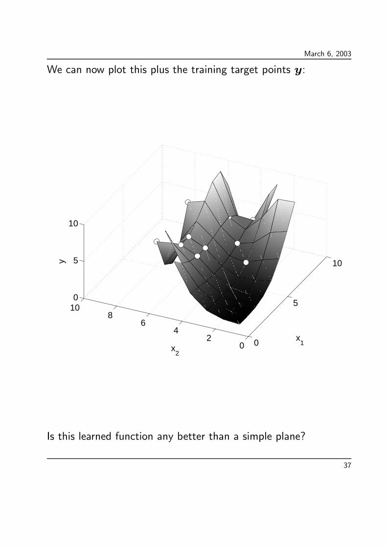
We can now plot this plus the training target points y:

0

5

10

02

46

8100

5

10

x1

x2

y

Is this learned function any better than a simple plane?

37

March 6, 2003

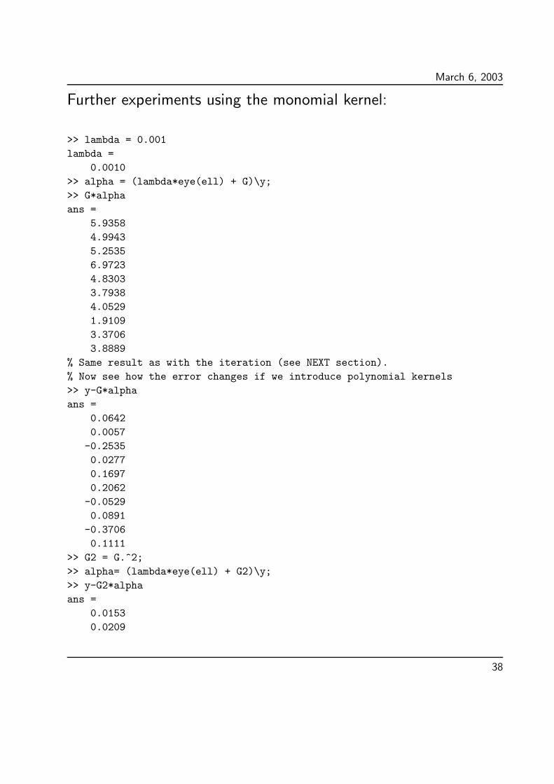
Further experiments using the monomial kernel:

>> lambda = 0.001

lambda =

0.0010

>> alpha = (lambda*eye(ell) + G)\y;

>> G*alpha

ans =

5.9358

4.9943

5.2535

6.9723

4.8303

3.7938

4.0529

1.9109

3.3706

3.8889

% Same result as with the iteration (see NEXT section).

% Now see how the error changes if we introduce polynomial kernels

>> y-G*alpha

ans =

0.0642

0.0057

-0.2535

0.0277

0.1697

0.2062

-0.0529

0.0891

-0.3706

0.1111

>> G2 = G.^2;

>> alpha= (lambda*eye(ell) + G2)\y;

>> y-G2*alpha

ans =

0.0153

0.0209

38

March 6, 2003

-0.0420

-0.0241

0.1429

-0.0253

0.0233

0.0892

-0.1594

-0.0366

>> G3 = G.^3;

>> alpha = (lambda*eye(ell) + G3)\y;

>> y-G3*alpha

ans =

-0.0010

0.0119

-0.0105

-0.0002

0.0028

-0.0143

0.0158

0.0041

-0.0090

0.0005

>> G4 = G.^4;

>> alpha = (lambda*eye(ell) + G4)\y;

>> y-G4*alpha

ans =

1.0e-003 *

-0.0128

0.1469

-0.1505

0.0126

-0.0067

-0.1437

0.1645

0.0046

-0.0206

0.0049

39

March 6, 2003

Steepest descent for regression - kernel version

Consider the basic iteration step:

wnew = wold + ηX′(y − Xwold

)

from this we have, if α = Xw that:

X′αnew = X

′αold + ηX

′(y − XX ′

αold

)

and thus if G = XX′then

Gαnew = Gαold + ηG(

y − Gαold

)

or if we assume that G is invertible that:

αnew = αold + η(

y − Gαold

)

This is the iteration step of the kernel version.

40

March 6, 2003

For the ridge-regression where we minimize

λ⟨

w · w⟩

+⟨

(y − Xw) · (y − Xw)⟩

the basic step in the original version becomes

wnew = wold + η(

X′(y − Xwold

)

− λwold

)

and in the kernel version

αnew = αold + η(

y −(

G+ λI`)

αold

)

41

March 6, 2003

% We try the kernel method on our regression dataset:

>> Xhat=[X ones(ell,1)]

Xhat =

3 7 1

4 6 1

5 6 1

7 7 1

8 5 1

4 5 1

5 5 1

6 3 1

7 4 1

9 4 1

>> G = Xhat*Xhat’

G =

59 55 58 71 60 48 51 40 50 56

55 53 57 71 63 47 51 43 53 61

58 57 62 78 71 51 56 49 60 70

71 71 78 99 92 64 71 64 78 92

60 63 71 92 90 58 66 64 77 93

48 47 51 64 58 42 46 40 49 57

51 51 56 71 66 46 51 46 56 66

40 43 49 64 64 40 46 46 55 67

50 53 60 78 77 49 56 55 66 80

56 61 70 92 93 57 66 67 80 98

>> y = [6 5 5 7 5 4 4 2 3 4]’ ;

>> alpha = zeros(10,1)

alpha =

0

0

0

0

0

0

0

0

0

0

42

March 6, 2003

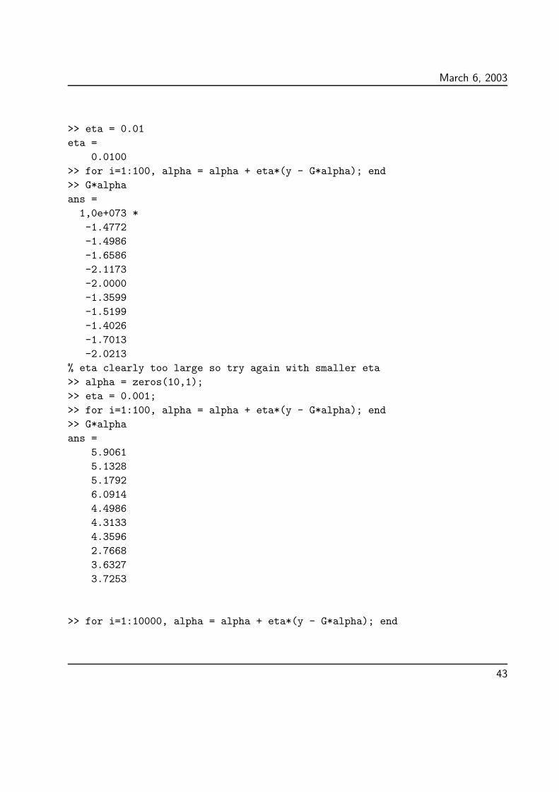
>> eta = 0.01

eta =

0.0100

>> for i=1:100, alpha = alpha + eta*(y - G*alpha); end

>> G*alpha

ans =

1,0e+073 *

-1.4772

-1.4986

-1.6586

-2.1173

-2.0000

-1.3599

-1.5199

-1.4026

-1.7013

-2.0213

% eta clearly too large so try again with smaller eta

>> alpha = zeros(10,1);

>> eta = 0.001;


>> G*alpha

ans =

5.9061

5.1328

5.1792

6.0914

4.4986

4.3133

4.3596

2.7668

3.6327

3.7253


43

March 6, 2003

>> G*alpha

ans =

5.9406

5.0193

5.2463

6.8484

4.7790

3.8711

4.0981

2.0286

3.4038

3.8577


>> G*alpha

ans =

5.9364

4.9973

5.2527

6.9580

4.8244

3.8027

4.0581

1.9245

3.3744

3.8852


>> G*alpha

ans =

5.9358

4.9940

5.2536

6.9741

4.8310

3.7927

4.0523

1.9092

3.3701

3.8893

44

March 6, 2003


>> G*alpha

ans =

5.9357

4.9935

5.2537

6.9765

4.8320

3.7912

4.0514

1.9069

3.3695

3.8899


>> alpha = alpha + eta*(y - G*alpha);

>> G*alpha

ans =

5.9357

4.9935

5.2538

6.9769

4.8322

3.7910

4.0513

1.9066

3.3694

3.8900

% We seem to have reached convergence after 40000 iterations!

45

March 6, 2003

1-norm regression

In chapter 2 we derived the following formulation:

min∑

i=1

ξ+i + ξ

−i

subject to Xw + ξ+ − ξ− = y and ξ+, ξ− ≥ 0.

The kernel version of the formulation will be exactly the same

except that the constraints become:

Gα+ ξ+ − ξ− = y

When re-solving the problem in chapter 2 using a polynomial

kernel, i.e. the (i, j)-the element of G, K(xi,xj), replaced

by K(xi,xj)d or (1 +K(xi,xj))

d we would again expect the

error vectors ξ+ and ξ+ to become smaller.

46

March 6, 2003

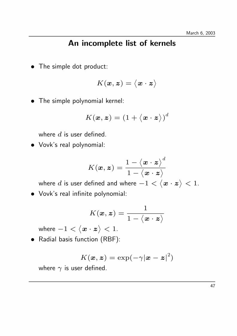
An incomplete list of kernels

• The simple dot product:

K(x, z) =⟨

x · z⟩

• The simple polynomial kernel:

K(x, z) = (1 +⟨

x · z⟩

)d

where d is user defined.

• Vovk’s real polynomial:

K(x, z) =1−

⟨

x · z⟩d

1−⟨

x · z⟩

where d is user defined and where −1 <⟨

x · z⟩

< 1.

• Vovk’s real infinite polynomial:

K(x, z) =1

1−⟨

x · z⟩

where −1 <⟨

x · z⟩

< 1.

• Radial basis function (RBF):

K(x, z) = exp(−γ|x− z|2)where γ is user defined.

47

March 6, 2003

• Two layer neural network (the sigmoid kernel):

K(x, z) =1

1 + exp(v⟨

x · z⟩

)− c

where v and c must satisfy Mercer’s condition (for example if

|x| = 1, |z| = 1 then c ≥ v.

• Linear splines with an infinite number of points:For the one-dimensional case:

Kk(x, z) = 1 + xz + xzmin(x, z)

−x+ z

2(min(xz))

2+

(min(x, z))3

3

for the multi-dimensional case

K(x, z) =

n∏

k=1

Kk(xk, zk)

• Full polynomial kernel:

K(x, z) =

(

⟨

x · z⟩

a+ b

)d

where a, b and d are user defined.

• Regularized Fourier (weaker mode regularization)

48

March 6, 2003

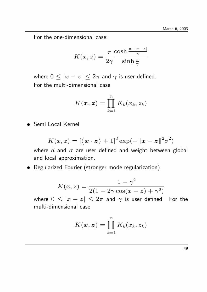
For the one-dimensional case:

K(x, z) =π

2γ

cosh π−|x−z|γ

sinh πγ

where 0 ≤ |x− z| ≤ 2π and γ is user defined.

For the multi-dimensional case

K(x, z) =

n∏

k=1

Kk(xk, zk)

• Semi Local Kernel

K(x, z) = [⟨

x · z⟩

+ 1]dexp(−‖x− z‖2σ2

)

where d and σ are user defined and weight between global

and local approximation.

• Regularized Fourier (stronger mode regularization)

K(x, z) =1− γ2

2(1− 2γ cos(x− z) + γ2)

where 0 ≤ |x − z| ≤ 2π and γ is user defined. For the

multi-dimensional case

K(x, z) =

n∏

k=1

Kk(xk, zk)

49

March 6, 2003

• Anova 1

K(x, z) = (

n∑

k=1

exp(−γ(xk − zk)2))d

where the degree d and γ are user defined.

50

March 6, 2003

Two layered neural network

The two layered neural network or sigmoid kernel deserved

some further remarks. Usually the two layered neural network

architecture is drawn as follows:

missing figure drawn in class

• The number of support vectors corresponds to the number ofhidden nodes,

• the weights of the hidden layer are the support vectors (x),• the weights of the output layer is α.

51

March 6, 2003

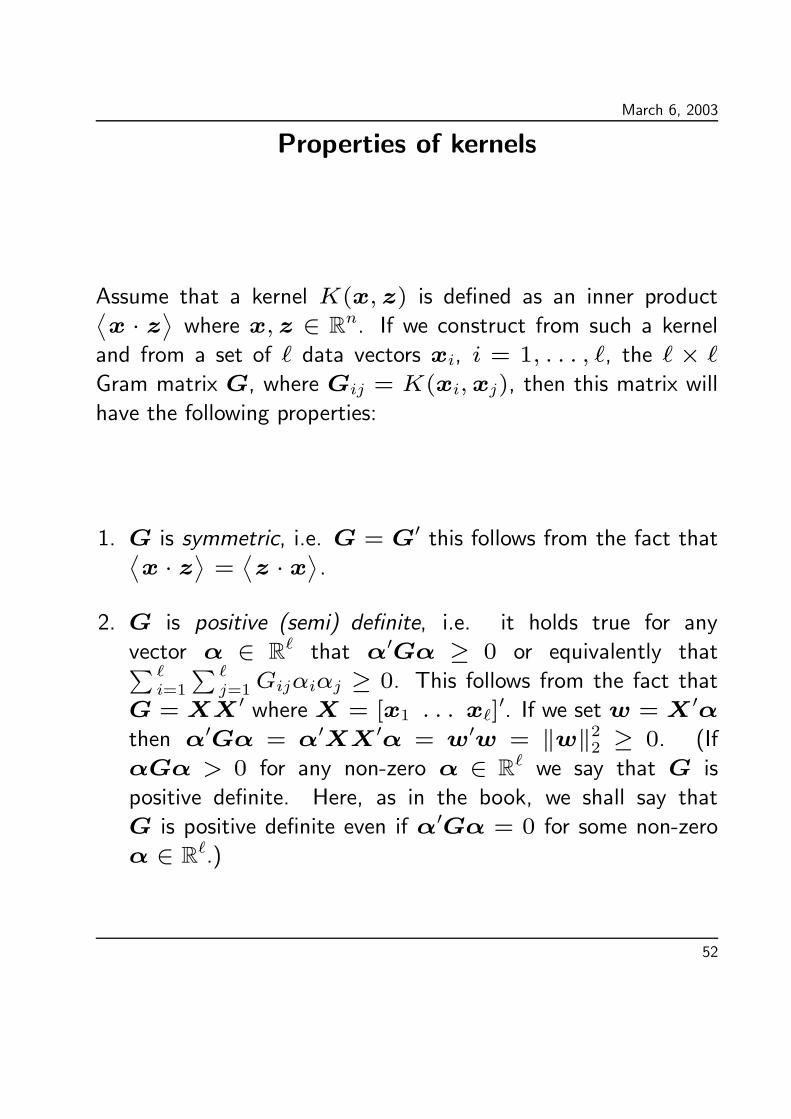
Properties of kernels

Assume that a kernel K(x, z) is defined as an inner product⟨

x · z⟩

where x, z ∈ Rn. If we construct from such a kernel

and from a set of ` data vectors xi, i = 1, . . . , `, the ` × `

Gram matrix G, where Gij = K(xi,xj), then this matrix will

have the following properties:

1. G is symmetric, i.e. G = G′ this follows from the fact that⟨

x · z⟩

=⟨

z · x⟩

.

2. G is positive (semi) definite, i.e. it holds true for any

vector α ∈ R` that α′Gα ≥ 0 or equivalently that∑`

i=1

∑`j=1Gijαiαj ≥ 0. This follows from the fact that

G = XX ′ whereX = [x1 . . . x`]′. If we set w = X ′α

then α′Gα = α′XX ′α = w′w = ‖w‖22 ≥ 0. (If

αGα > 0 for any non-zero α ∈ R` we say that G is

positive definite. Here, as in the book, we shall say that

G is positive definite even if α′Gα = 0 for some non-zero

α ∈ R`.)

52

March 6, 2003

When a kernel K(x, z) is not defined explicitly as an inner

product, the two properties above must be preserved when we

construct the Gram matrix from the kernel. Note that in this

case the space of data vectors, D, is not necessarily Rn for any n.

The first property is preserved if K(x, z) = K(z,x) for all

x,y ∈ D. In this case we say that the kernel K is symmetric.

The second property is preserved if

∫

D

∫

DK(x, z)f(x)f(z)dxdz ≥ 0

where f is any function defined on the data space with properties

that make the integral mathematically meaningful. In this case

we say that the kernel K is (semi) positive (cf. theorem 3.6 p.

35).

A kernel satisfying these two conditions is called aMercer kernel.

Note that if we choose f as a weighted sum of delta functions at

x1,x2, . . . ,x` ∈ D. with the weights α1, α2, . . . , α` then the

double integral reduces to the double sum:

∑

i=1

∑

j=1

K(xi,xj)αiαj

53

March 6, 2003

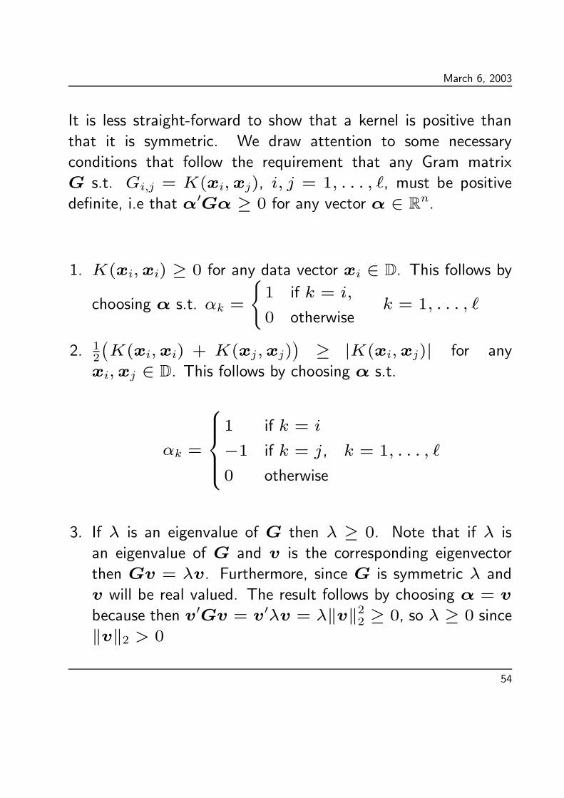
It is less straight-forward to show that a kernel is positive than

that it is symmetric. We draw attention to some necessary

conditions that follow the requirement that any Gram matrix

G s.t. Gi,j = K(xi,xj), i, j = 1, . . . , `, must be positive

definite, i.e that α′Gα ≥ 0 for any vector α ∈ Rn.

1. K(xi,xi) ≥ 0 for any data vector xi ∈ D. This follows by

choosing α s.t. αk =

{

1 if k = i,

0 otherwisek = 1, . . . , `

2. 12

(

K(xi,xi) + K(xj,xj))

≥ |K(xi,xj)| for any

xi,xj ∈ D. This follows by choosing α s.t.

αk =

1 if k = i

−1 if k = j, k = 1, . . . , `

0 otherwise

3. If λ is an eigenvalue of G then λ ≥ 0. Note that if λ is

an eigenvalue of G and v is the corresponding eigenvector

then Gv = λv. Furthermore, since G is symmetric λ and

v will be real valued. The result follows by choosing α = v

because then v′Gv = v′λv = λ‖v‖22 ≥ 0, so λ ≥ 0 since

‖v‖2 > 0

54

March 6, 2003

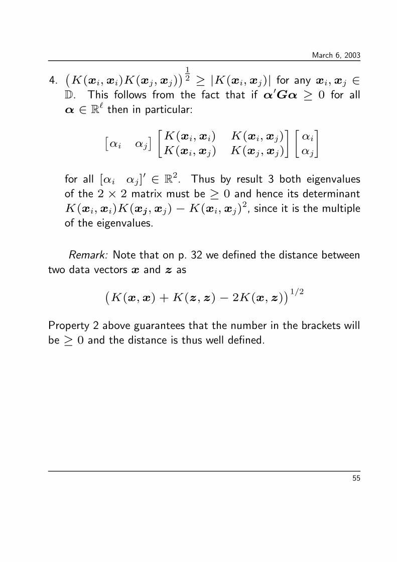
4.(

K(xi,xi)K(xj,xj))

12 ≥ |K(xi,xj)| for any xi,xj ∈

D. This follows from the fact that if α′Gα ≥ 0 for all

α ∈ R` then in particular:

[

αi αj]

[

K(xi,xi) K(xi,xj)

K(xi,xj) K(xj,xj)

] [

αiαj

]

for all [αi αj]′ ∈ R2. Thus by result 3 both eigenvalues

of the 2 × 2 matrix must be ≥ 0 and hence its determinant

K(xi,xi)K(xj,xj)−K(xi,xj)2, since it is the multiple

of the eigenvalues.

Remark: Note that on p. 32 we defined the distance between

two data vectors x and z as

(

K(x,x) +K(z, z)− 2K(x, z))1/2

Property 2 above guarantees that the number in the brackets will

be ≥ 0 and the distance is thus well defined.

55

March 6, 2003

Features from kernels

Suppose we have constructed an ` × ` Gram matrix G from a

symmetric and positive kernel K(x, z), s.t. Gij = K(xi,xj),

i, j = 1, . . . , `, and we are now interested in defining feature

vectors φ(xi), i = 1, . . . , ` such that

K(xi,xj) =⟨

φ(xi) · φ(xj)⟩

Since G will be symmetric and positive definite it will have `

real non-negative eigenvalues λ1, λ1, . . . , λ` and corresponding

eigenvectors v1, . . . ,v`. Moreover, these eigenvectors will be

mutually orthogonal, i.e.⟨

vi · vj⟩

= 0 if i 6= j and they can

be normalized s.t.⟨

vi · vi⟩

= 1 for i = 1, . . . , `.

It follows that if V is the `× ` matrix [v1 v2 . . .v`] then

GV = V

λ1 0. . .

0 λ`

= V Λ

and hence G = V ΛV ′. Hence, if we set V = V√Λ, i.e.

multiply the first column of V with√λ1 the second one with√

λ2 and so on, then

G = V V′

Thus we can define φ(xi)′ to be the i-th row of V ,

i = 1, . . . , `.

56

March 6, 2003

Note that the MATLAB function

[V, Lambda] = eig(G);

gives us the matrix of eigenvectors, V , and the diagonal matrix

of eigenvalues, Λ. Thus the matrix whose rows are feature

vectors corresponding to G will be

Vhat = V*sqrt(Lambda);

57

March 6, 2003

Making kernels from kernels

Let K1 and K2 be kernels over X ×X, X ⊆ Rn, a ∈ R+,

f(·) a real-valued function on X, φ : X 7→ Rm with kernel

K3 a kernel over Rm × Rm, and B a symmetric positive (semi)

definite n× n matrix. Then the following functions are kernels:

• K(x, z) = K1(x, z) +K2(x, z)

• K(x, z) = a+K1(x, z)

• K(x, z) = aK1(x, z)

• K(x, z) = K1(x, z)K2(x, z)

• K(x, z) = f(x)f(z)

• K(x, z) = exp (K1(x, z))

• K(x, z) = p(

K1(x, z))

• K(x, z) = K3

(

φ(x),φ(z))

• K(x, z) = x′Bz

where p(x) is a polynomial with positive coefficients.

58

March 6, 2003

Feature selection revisited

The task of feature extraction is highly problem-dependent and

for different domains the features may be completely different.

In many real world problems feature extraction can only be

partially automated, and the knowledge of human experts

remains indispensable.

In real world applications the number of features is often large.

The goal of feature selection is to reduce this dimensionality by

selecting only a subset of features.

There are in principle to approaches to finding a good feature

subset:

• search the feature space using the learning algorithm’s

estimated accuracy as a search criteria (e.g. cross validation),

or

• use a criteria which is “independent” of the learning algorithm(e.g. compute correlation between feature and target).

59

March 6, 2003

Extracting regularities from attributes

If some regularities in the input attributes are known, then they

can be exploited by creating so called locality-improved kernels.

For example:

• In real world images, correlations over short distance are muchmore reliable features than long-range correlations.

• Genomic sequences contain untranslated regions and CDSregions which encode for proteins. An important task is

therefore to recognize translation initiation sites (TIS). We

know that a TIS usually starts with a ATG code sequence and

so a local correlation using a window around ATG has shown

to be very successful when designing locality-improved kernels

for the DNA start codon recognition task.

In general the locality-improved kernel may be written as follows:

K(x, z) =

(

∑

locality

(

∑

i∈locality

f(xi, zi)

)d1)d2

using a monomial type kernel. Other variation are also

possible. The function f is a simple multiplication for the image

classification problem and a matching operation for the TIS

recognition problem.

60

March 6, 2003

Reproducing Kernel Hilbert Spaces

Let a before X ⊆ Rn denote an input space of possible

n-dimensional input vectors x = (x1, . . . , xn), φ denote the

mapping that maps each x ∈ X into an N -dimensional feature

vector φ(x) =(

φ1(x), . . . , φN(x))

, and K(x,y) denote a

(Mercer) kernel function defined on X×X such thatK(x,y) =⟨

φ(x) · φ(x)⟩

, the inner product of the feature vectors φ(x)

and φ(y) in the feature space F = {φ(x)|x ∈ X} ⊆ RN

Rather than associating with a given input vector x ∈ X its

feature vector φ(x) it is sometimes instructive to associate with

it the function∑N

i=1 φi(x)φi(x) = K(x,x) defined on X(note that here x is a fixed vector but x is a variable) which

contains information on the “relationship” between x and all

other input vectors x ∈ X .

61

March 6, 2003

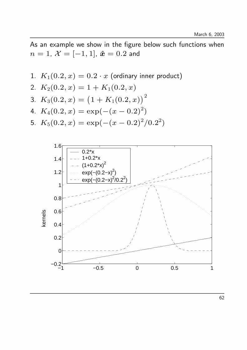
As an example we show in the figure below such functions when

n = 1, X = [−1, 1], x = 0.2 and

1. K1(0.2, x) = 0.2 · x (ordinary inner product)2. K2(0.2, x) = 1 +K1(0.2, x)

3. K3(0.2, x) =(

1 +K1(0.2, x))2

4. K4(0.2, x) = exp(−(x− 0.2)2)

5. K5(0.2, x) = exp(−(x− 0.2)2/0.22)

−1 −0.5 0 0.5 1−0.2

0

0.2

0.4

0.6

0.8

1

1.2

1.4

1.6

kern

els

0.2*x1+0.2*x(1+0.2*x)2

exp(−(0.2−x)2)exp(−(0.2−x)2/0.22)

62

March 6, 2003

For ` training vectors x1,x2, . . . ,x` ∈ X the binary

classification problem becomes in this context the problem

of finding ` real numbers α1, α2, . . . , α`, and b such that if we

form the function

f(x) =∑

i=1

αiK(xi,x)

f(xi) + b > 0 if xi is in the + class and

f(xi) + b < 0 if xi is in the − class, where b is a possible

offset value. This follows directly from the dual formulation of

this problem.

Example: It becomes clear in this context that if we take the

kernel to be K(x,y) = exp(−‖x − y‖2/σ2) and choose σ

sufficiently small , we can solve the binary classification problem

for the training set simply by setting αi = 1 if xi is in the +

class, αi = −1 if x is in the − class, and b = 0.

63

March 6, 2003

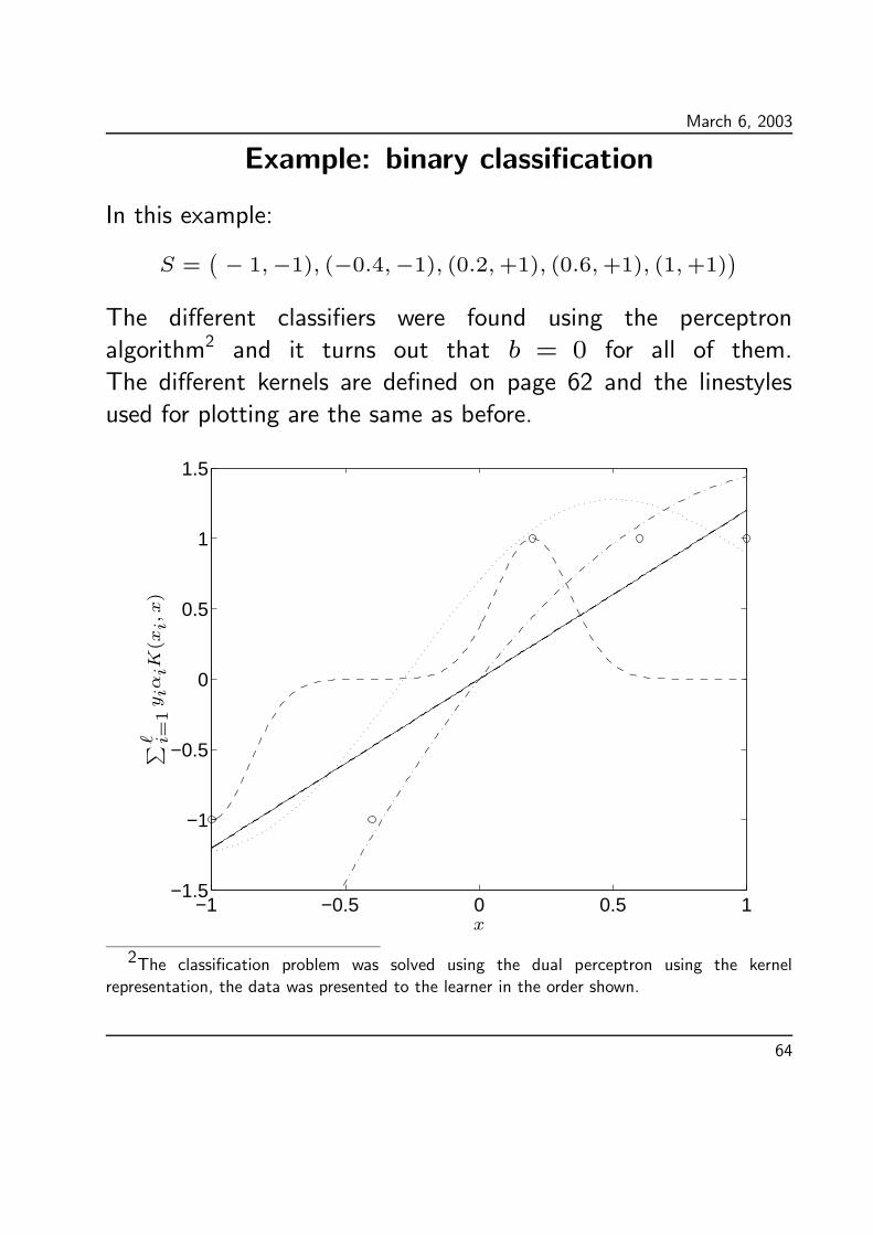
Example: binary classification

In this example:

S =(

− 1,−1), (−0.4,−1), (0.2,+1), (0.6,+1), (1,+1))

The different classifiers were found using the perceptron

algorithm2 and it turns out that b = 0 for all of them.

The different kernels are defined on page 62 and the linestyles

used for plotting are the same as before.

−1 −0.5 0 0.5 1−1.5

−1

−0.5

0

0.5

1

1.5

PSfrag replacements

∑

` i=1yiαiK

(xi,x)

x

2The classification problem was solved using the dual perceptron using the kernel

representation, the data was presented to the learner in the order shown.

64

March 6, 2003

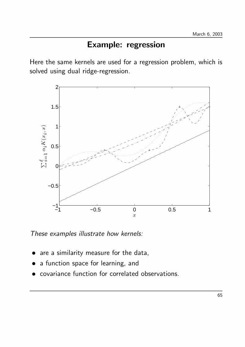
Example: regression

Here the same kernels are used for a regression problem, which is

solved using dual ridge-regression.

−1 −0.5 0 0.5 1−1

−0.5

0

0.5

1

1.5

2

PSfrag replacements

∑

` i=1αiK

(xi,x)

x

These examples illustrate how kernels:

• are a similarity measure for the data,• a function space for learning, and• covariance function for correlated observations.

65

March 6, 2003

Similarly the regression problem becomes to find ` real numbers

α1, α2, . . . , α` such that f(xi) ≈ yi for i = 1, 2, . . . , `

where yi, i = 1, 2, . . . , ` are given outputs values.

In this context we also consider the space of all functions

a(x) =

N∑

i=1

aiφi(x)

where ai ∈ R and denote it by H. We can define for any twofunctions a(x) =

∑Ni=1 aiφi(x) and b(x) =

∑Ni=1 biφi(x)

their inner product as the value

N∑

i=1

aibi.

Thus H becomes an inner product space and in fact a Hilbert

space (since it will also be complete). We denote this inner

product by⟨

a(x) · b(x)⟩

H and define the corresponding norm:

‖a(x)‖H =⟨

a(x) · a(x)⟩1/2

H =(

N∑

i=1

a2i

)1/2

66

March 6, 2003

Note that according to these definitions we have

1.⟨

K(xi,x) ·K(xj,x)⟩

H=⟨∑N

k=1 φk(xi)φk(x) ·∑N

k=1 φk(xj)φk(x)⟩

H=∑N

k=1 φk(xi)φk(xj) = K(xi,xj)

2. If f(x) =∑`

i=1 αiK(xi,x)

and g(x) =∑`

i=1 βiK(xi,x) then⟨

f(x) · g(x)⟩

H =∑`

i=1

∑`j=1 αiβjK(xi,xj) = α′Gβ

where α = (α1, . . . , α`)′, β = (β1, . . . , β`)

′ and G is an

` × ` Gram (kernel) matrix whose (i, j)-th element is the

kernel K(xi,xj). In particular ‖f(x)‖2H = α′Gα.

3.⟨

a(x) ·K(y,x)⟩

H=⟨∑N

i=1 aiφi(x) ·∑N

i=1 φi(y)φi(x)⟩

H=∑N

i=1 aiφi(y) = a(y)

A kernel with this last property is called a reproducing

kernel. Thus H is called a reproducing kernel Hilbert

space (RKHS).

The above definitions agree with those given on p. 38-40 in book

except in the book N = ∞ and the book further considers a

more general case where we introduce positive weight factors µi,

which above simply take the value 1.

67

March 6, 2003

Principle component analysis (PCA)

Let Φ denote a data matrix in feature space for ` data vectors

x1,x2, . . . ,x`, i.e. the i-th row of Φ is φ(xi)′.

Let Φ denote the corresponding matrix of centered data where

we have subtracted from the j-th component of φ(xi), i.e.

φi(xi), the average value of that component over the dataset so

that the (i, j)-the element of Φ is

φj(xi)− 1`

∑

i=1

φj(xi)

In matrix notation we have that

Φ = Φ− 1èe

′Φ

where e denotes a column vector of ` 1-elements. This implies

that

ΦΦ′= ΦΦ

′ − 1èe

′ΦΦ

′ − ΦΦ′1èe′+ 1

èe′ΦΦ

′1èe

′

and shows how we can obtain the Gram matrix from features

in centered form from the Gram matrix with its data in original

form.

68

March 6, 2003

We are now interested in extracting from the centered feature

vectors a new feature vector which is a linear combination of

the original features but with the additional property that the

variance in these new feature values is as large as possible. In

this way the new feature is to incorporate as much information

as possible from older features. We refer to it as a principle

component of the data. Thus we are interested in finding a

weight vector w, s.t. ‖w‖2 = 1 but

1`

⟨

Φw · Φw⟩

= w′1`ΦΦ

′w

is maximized3. Note that 1`Φ

′Φ is the covariance of the original

features.

The solution to the above problem is well known. We choose w

as the eigenvector of the covariance matrix that corresponds to

the largest eigenvalue λmax and normalize it so that ‖w‖2 = 1.

Then w′1`Φ′Φw = w′λmaxw = λmax, i.e. the variance of

the new feature will be λmax and this is the largest possible

variance.

3Compare this with the classification problem where we are interested in finding a weightvector s.t. ‖w‖2 = 1 and such that

⟨

xi ·w⟩

> 0 for all xi data vectors in the +-class

and⟨

xi ·w⟩

< 0 for all xi data vectors in the −-class. In that problem we also includedan offset b but if we work with centered data the offset value will in many cases become 0.Also compare it with the regression problem where we are interested in finding the weight

vector s.t.⟨

xi ·w⟩

≈ yi for some output values yi, i = 1, . . . , `.

69

March 6, 2003

Our main problem is however that in many cases we do not

know the new feature vectors explicitly and thus cannot compute

their average values nor the covariance matrix. We do however

know the Gram matrix ΦΦ′ whose (i, j)-th element is the kernelk(xi,xj) and can therefore also calculate the Gram-matrix of

the centered feature values as shown above.

We also have the following result:

• If λ is a non-zero eigenvalue of the matrix ΦΦ′with

eigenvector α then λ is also a non-zero eigenvalue of the

matrix Φ′Φ with eigenvector w = Φ

′α, since

ΦΦ′α = λα ⇒ Φ

′Φ(Φ′α) = λ(Φ′α).

• Conversely if λ is a non-zero eigenvalue of the matrix Φ′Φwith eigenvector w then λ will also be a non-zero eigenvalue

of the matrix ΦΦ′with eigenvector α = Φw.

• Note that the matrices Φ′Φ and ΦΦ′will in general be of

different size so that one will have more eigenvalues than

the other. The result above implies that all such additional

eigenvalues will be 0.

70

March 6, 2003

We can now calculate the largest eigenvalue λmax of the

covariance matrix 1`Φ

′Φ by calculating the eigenvalues of 1

`G,

where G denotes the Gram matrix ΦΦ′. Let αmax denote

the corresponding eigenvector. Since we want to normalize w

s.t.⟨

w ·w⟩

= 1 and w = Φ′α this means that we want to

normalize α s.t.

α′ΦΦ

′α = α

′`λmaxα = `λmaxα · α = 1

i.e. such that ‖α‖2 = 1/√`λmax.

We can however in general not calculate w for the expression

w = Φ′α since we do not know the feature vector explicitly.

This is analogous to the situation in kernel classification and

regression and we can deal with it in the same way, i.e. for a new

x we calculate the corresponding feature value as

∑

i=1

K(xi,x)αi

where αi is the i-the component of the eigenvector α after it

has been normalized (as shown above) and K(z,x) is the kernel

value corresponding to centered feature values.

In particular, the vector of the feature principal component values

71

March 6, 2003

of out data will be:

Gα = `λmaxα

(since α is an eigenvector of G and `λmax is the corresponding

eigenvalue), i.e. the eigenvector normalized so that its length is

`λmax1√

`λmax=√

`λmax

Note that this corresponds to the results on page 56.

It is, however, not clear how to proceed when if we want to

calculate the principle component for a new data vector. Also

note that the eigenvectors of the Gram matrix G will in general

not be sparse, i.e. most of the αi values will be non-zero. To

obtain a sparse α-vector we may have to modify our formulation

in some way. Such modified principle components are called

sparse principle components.

We do not necessarily restrict our attention only to the extracted

feature corresponding to the largest variance. Another feature

may be extracted from the eigenvector of 1`G corresponding to

the second largest eigenvalue. This second feature is uncorrelated

with the first feature and so incorporates information ignored by

the first feature. We call this second feature a second principle

component. Similarly, we can extract a third principle component

and so on.

72

March 6, 2003

Note that the total variance in the original data after it has been

transformed into the feature space is the sum of the diagonal

entries of the covariance matrix 1`Φ

′Φ. We can however not

calculate this metric if the features are not explicitly known.

But it can be shown that this sum is the same as the sum of

the diagonal entries of he matrix 1`G which can be calculated

from the kernels and is also equal to the sum of the eigenvalues

of this matrix. Thus by comparing the sum of the largest p

eigenvalues, say, with the total variance, we can see how much of

the information in the original data is incorporated into the first

p principle components in feature space.

The following MATLAB function performs the calculationsdescribed so far:

function [P,Pvar,totvar] = principalfeatures(G,p);

%PRINCIPLEFEATURES

% usage: [P,Pvar,totvar] = principalfeatures(G,p);

% P are the principle components

% Pvar the corresponding eigenvalues and totvar is the total variance

% G is the Gram matrix and p the number of principle components

ell = size(G,1);

Gbar = ((1/ell)*ones(ell,1))*(ones(1,ell)*G);

Gbar = G - Gbar - ((G - Gbar)*ones(ell,1))*((1/ell)*ones(1,ell));

[V,Lambda] = eigs((1/ell)*Gbar,p);

P = V*sqrt(ell*Lambda);

Pvar = diag(Lambda);

totvar = (1/ell)*sum(diag(Gbar));

% make sure that the largest eigenvalues are first!

[dummy,I] = sort(-Pvar);

Pvar = Pvar(I);

P = P(:,I);

73

March 6, 2003

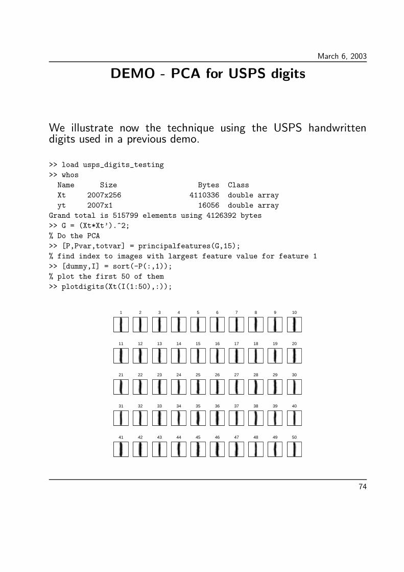
DEMO - PCA for USPS digits

We illustrate now the technique using the USPS handwrittendigits used in a previous demo.

>> load usps_digits_testing

>> whos

Name Size Bytes Class

Xt 2007x256 4110336 double array

yt 2007x1 16056 double array

Grand total is 515799 elements using 4126392 bytes

>> G = (Xt*Xt’).^2;

% Do the PCA

>> [P,Pvar,totvar] = principalfeatures(G,15);

% find index to images with largest feature value for feature 1

>> [dummy,I] = sort(-P(:,1));

% plot the first 50 of them

>> plotdigits(Xt(I(1:50),:));

1 2 3 4 5 6 7 8 9 10

11 12 13 14 15 16 17 18 19 20

21 22 23 24 25 26 27 28 29 30

31 32 33 34 35 36 37 38 39 40

41 42 43 44 45 46 47 48 49 50

74

March 6, 2003

What if we skip every 40-th image and so show a sample of allimages sorted by the first principle component feature value:

>> plotdigits(Xt(I(1:40:end),:));

1 2 3 4 5 6 7 8 9 10

11 12 13 14 15 16 17 18 19 20

21 22 23 24 25 26 27 28 29 30

31 32 33 34 35 36 37 38 39 40

41 42 43 44 45 46 47 48 49 50

Notice that at the other end of the scale we have only zeros!Let’s try another kernel (monomial order 5):

>> G = (Xt*Xt’).^5;


>> [dummy,I] = sort(-P(:,1));

>> plotdigits(Xt(I(1:40:end),:));

This time the zeros are first:

1 2 3 4 5 6 7 8 9 10

11 12 13 14 15 16 17 18 19 20

21 22 23 24 25 26 27 28 29 30

31 32 33 34 35 36 37 38 39 40

41 42 43 44 45 46 47 48 49 50

75

March 6, 2003

Finally, let us plot the images with the highest feature value forall 15 principle components extracted using a order 2 monomialkernel:

>> G = (Xt*Xt’).^2;


>> Pvar

Pvar =

1.0e+03 *

4.8461

2.4100

1.6495

1.2537

1.1182

1.0137

0.8469

0.7460

0.6618

0.6380

0.5479

0.4504

0.4491

0.4129

0.3808

>> for i=1:15, [dummy,I] = sort(P(:,i)); Iext(i,:) = [I(1) I(end)]; end

>> figure(1); plotdigits(Xt(Iext(:,1),:),yt(Iext(:,1)),(1:15)’);

>> figure(2); plotdigits(Xt(Iext(:,2),:),yt(Iext(:,2)),-(1:15)’);

0(1) 9(2) 0(3) 8(4) 3(5) 0(6) 4(7) 2(8) 6(9) 5(10)

1(11) 2(12) 3(13) 0(14) 3(15)

1(−1) 6(−2) 0(−3) 2(−4) 6(−5) 2(−6) 7(−7) 9(−8) 9(−9) 5(−10)

6(−11) 3(−12) 7(−13) 4(−14) 5(−15)

Notice that almost all digits are represented by the first 15 PC.

76

March 6, 2003

PCA - unsupervised learning

In general PCA may be regarded as an unsupervised learning

technique.

Classroom discussion on Kernel PCA in kernel design.

77

March 6, 2003

Designing kernels

Designing a kernel corresponds to choosing a:

• similarity measure for the data,• linear representation of the data,• function space for learning,• covariance function for correlated observations.

In general, the choice of kernel reflects the designer’s knowledge

about the problem and its solution.

There is no free lunch in kernel choice!

78

Kernel-Induced Feature Spaces - University of Iceland · Kernel-Induced Feature Spaces Chapter3...

Documents

Transcript of Kernel-Induced Feature Spaces - University of Iceland · Kernel-Induced Feature Spaces Chapter3...