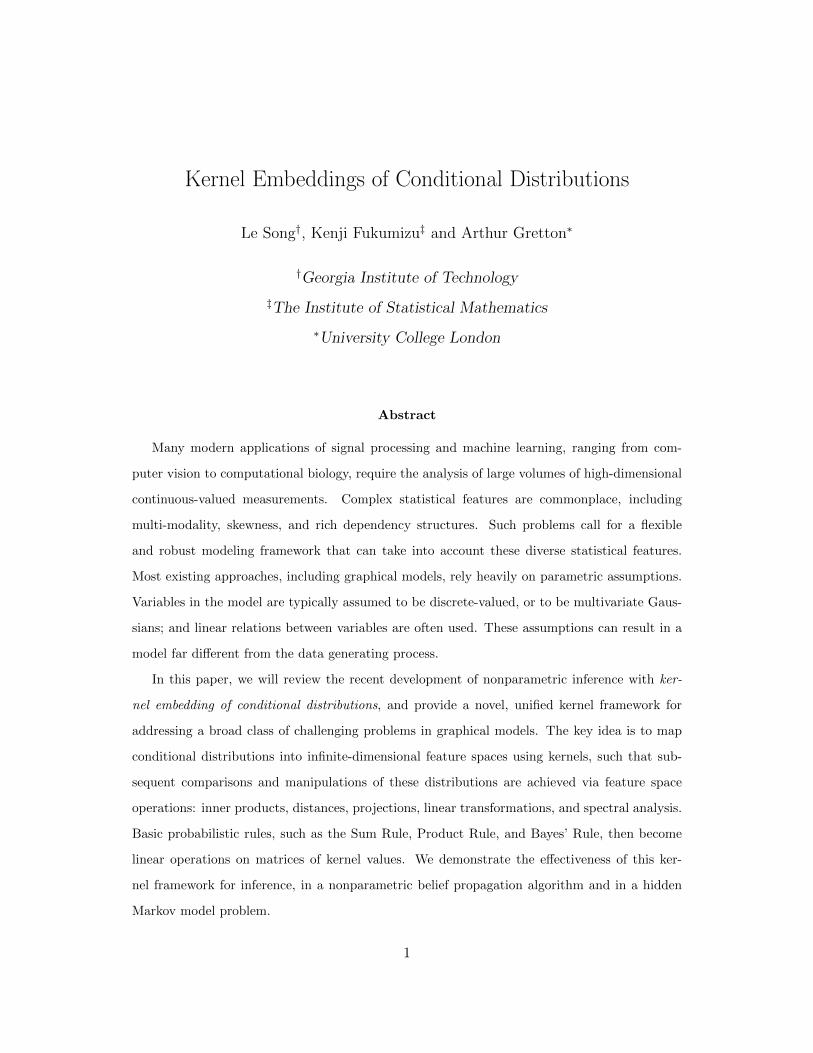
Kernel Embeddings of Conditional Distributions

Le Song†, Kenji Fukumizu‡ and Arthur Gretton∗

†Georgia Institute of Technology

‡The Institute of Statistical Mathematics

∗University College London

Abstract

Many modern applications of signal processing and machine learning, ranging from com-

puter vision to computational biology, require the analysis of large volumes of high-dimensional

continuous-valued measurements. Complex statistical features are commonplace, including

multi-modality, skewness, and rich dependency structures. Such problems call for a flexible

and robust modeling framework that can take into account these diverse statistical features.

Most existing approaches, including graphical models, rely heavily on parametric assumptions.

Variables in the model are typically assumed to be discrete-valued, or to be multivariate Gaus-

sians; and linear relations between variables are often used. These assumptions can result in a

model far different from the data generating process.

In this paper, we will review the recent development of nonparametric inference with ker-

nel embedding of conditional distributions, and provide a novel, unified kernel framework for

addressing a broad class of challenging problems in graphical models. The key idea is to map

conditional distributions into infinite-dimensional feature spaces using kernels, such that sub-

sequent comparisons and manipulations of these distributions are achieved via feature space

operations: inner products, distances, projections, linear transformations, and spectral analysis.

Basic probabilistic rules, such as the Sum Rule, Product Rule, and Bayes’ Rule, then become

linear operations on matrices of kernel values. We demonstrate the effectiveness of this ker-

nel framework for inference, in a nonparametric belief propagation algorithm and in a hidden

Markov model problem.

1

1 Introduction

A great many real-world signal processing problems exhibit complex statistical features, including

multi-modality, skewness, nonlinear relations, and sophisticated dependency structures. For in-

stance, in constructing depth maps from 2D images, the image features are high-dimensional and

continuous valued, and the depth is both continuous valued and has a multi-modal distribution

(Figure 1(a)). In predicting a sequence of camera movements from videos, the orientations of the

camera are continuous and non-Euclidean, and are predicted from continuous video features (Fig-

ure 1(b)). There is a common need for a flexible and robust modeling framework which can take

into account these diverse statistical features, as well as modeling the long-range and hierarchical

dependencies among the variables.

Pre

dic

t

depth

den

sity

𝑚𝑢1𝑡(𝑥𝑡) 𝑚𝑢2𝑡(𝑥𝑡)

𝑚𝑡𝑠(𝑥𝑠)

𝜷𝒖𝟐𝒕 =

𝛽𝑢2𝑡1 , … , 𝛽𝑢2𝑡

𝑚 ⊤

𝜷𝒖𝟏𝒕 = 𝛽𝑢1𝑡1 , … , 𝛽𝑢1𝑡

𝑚 ⊤

𝜷𝒕𝒔 = 𝛽𝑡𝑠1 , … , 𝛽𝑡𝑠

𝑚 ⊤

𝑋𝑢2

𝑋𝑢3

𝑋𝑢1

𝑋𝑡 𝑋𝑠

Outcoming message:

Prior 𝑃(𝑆𝑡−1|ℎ𝑡−1)

Likelihood 𝑃(𝑂𝑡|𝑆𝑡)

Posterior 𝑃(𝑆𝑡|ℎ𝑡−1𝑜𝑡)

𝜶𝒕−𝟏 = 𝛼1𝑡−1, … , 𝛼𝑚

𝑡−1 ⊤ 𝜶𝒕 = 𝛼1𝑡 , … , 𝛼𝑚

𝑡 ⊤ Prior Posterior

𝑆𝑡−1 𝑆𝑡

𝑜𝑡 𝑜𝑡−1

𝑆𝑡+1

𝑜𝑡+1

(a) Predicting depth from 2D image (b) Predicting camera orientation from video

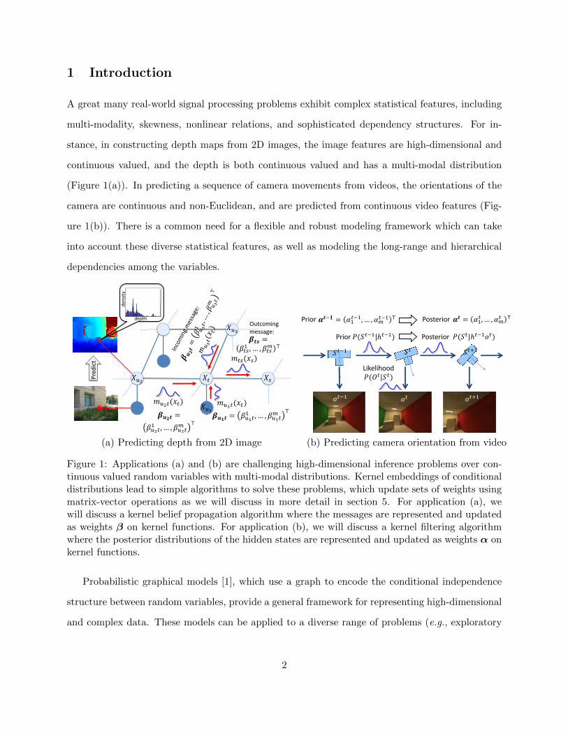
Figure 1: Applications (a) and (b) are challenging high-dimensional inference problems over con-tinuous valued random variables with multi-modal distributions. Kernel embeddings of conditionaldistributions lead to simple algorithms to solve these problems, which update sets of weights usingmatrix-vector operations as we will discuss in more detail in section 5. For application (a), wewill discuss a kernel belief propagation algorithm where the messages are represented and updatedas weights β on kernel functions. For application (b), we will discuss a kernel filtering algorithmwhere the posterior distributions of the hidden states are represented and updated as weights α onkernel functions.

Probabilistic graphical models [1], which use a graph to encode the conditional independence

structure between random variables, provide a general framework for representing high-dimensional

and complex data. These models can be applied to a diverse range of problems (e.g., exploratory

2

data analysis, feature extraction, handling missing values) using a common toolbox of learning and

inference algorithms. That said, most existing graphical modeling tools rely heavily on parametric

assumptions, such as discrete or multivariate Gaussian variables and linear relations. It remains

challenging to handle more complex distributions in a data-driven fashion.

A range of approaches exist to capture rich statistical features in data. A common way to model

higher-order statistical structures is to use high-dimensional nonlinear transformations, for instance

the polynomial mapping (x, y, z) 7→ (x, y, z, xy, yz, xz, x2, y2, z2, x3, y3 . . .) of the original variables.

The number of such nonlinear features explodes exponentially in high dimensions, however, which

limits the approach. Another representation for multi-modal distributions is as a finite mixture

of Gaussians, but this approach also suffers from drawbacks. First, fitting a mixture of Gaussians

is a non-convex problem, and it is often carried out using the Expectation-Maximization (EM)

algorithm, leading to a local optimum. Second, the EM algorithm can be slow to converge, especially

for high-dimensional data. Third, using a mixture of Gaussians in a graphical model inference

algorithm creates significant computational challenges [2], as we will see in our later example on

belief propagation. In this case, sampling or ad hoc approximations will be needed to make the

problem computationally tractable, which can be slow and lack guarantees.

There exist additional methods for modeling arbitrary distributions nonparametrically, without

using predefined polynomial features or a fixed number of Gaussians. Kernel density estimation

is among the most famous approaches along these lines, yet it is well known that this approach is

not suitable for high-dimensional data [3], and it typically does not take the dependence structure

among the variables into account. It is also possible to use the characteristic function, which

is the Fourier transform of a probability distribution function, to uniquely represent probability

distributions. This approach also suffers in high dimensions, where an empirical estimate based on

finite samples is not straightforward.

In this paper, we will review the recent development of nonparametric inference with kernel

embeddings of conditional distributions [4, 5, 6, 7, 8, 9, 10, 11, 12], and provide a novel, unified

kernel framework for addressing a broad class of challenging problems in graphical models. The

key idea of this line of work is to implicitly map (conditional or marginal) distributions into infinite

3

𝑃(𝑋)

𝜇𝑋 ≔ 𝔼𝑋[𝜙(𝑋)]

𝑃(𝑋, 𝑌)

𝒞𝑋𝑌 ≔ 𝔼𝑋𝑌[𝜙 𝑋 ⊗𝜙(𝑌)]

𝑃(𝑋, 𝑌, 𝑍)

𝒞𝑋𝑌𝑍 ≔ 𝔼𝑋𝑌𝑍[𝜙 𝑋 ⊗𝜙 𝑌 ⊗𝜙 𝑍 ]

𝑑𝑋 × 1

∞× 1

𝑑𝑋 × 𝑑𝑌

∞×∞

𝑑𝑋 × 𝑑𝑌 × 𝑑𝑍

∞×∞×∞

𝑋

𝑃(𝑋)

𝑋

𝑌 𝑃(𝑋, 𝑌)

𝑌

𝑋

𝑍 𝑃(𝑋, 𝑌, 𝑍)

𝑆𝑢𝑚 𝑅𝑢𝑙𝑒: 𝑄 𝑋 = 𝑃 𝑋 𝑌 𝜋(𝑌)

𝑌

𝑃𝑟𝑜𝑑𝑢𝑐𝑡 𝑅𝑢𝑙𝑒: 𝑄 𝑋, 𝑌 = 𝑃 𝑋 𝑌 𝜋(𝑌)

𝐵𝑎𝑦𝑒𝑠 𝑅𝑢𝑙𝑒: 𝑄 𝑌|𝑥 =𝑃 𝑥 𝑌 𝜋(𝑌)

𝑄(𝑋)

𝑆𝑢𝑚 𝑅𝑢𝑙𝑒: 𝜇𝑋𝜋 = 𝒞𝑋|𝑌𝜇𝑌

𝜋

𝑃𝑟𝑜𝑑𝑢𝑐𝑡 𝑅𝑢𝑙𝑒: 𝒞𝑋𝑌𝜋 = 𝒞𝑋|𝑌𝒞𝑌𝑌

𝜋

𝐵𝑎𝑦𝑒𝑠 𝑅𝑢𝑙𝑒: 𝜇𝑌|𝑥𝜋 = 𝒞𝑌|𝑋

𝜋 𝜙(𝑥)

𝜇𝑋 𝜇𝑌

𝒞𝑌|𝑋

Discrete

Kernel Embedding

Distributions Probabilistic Operations

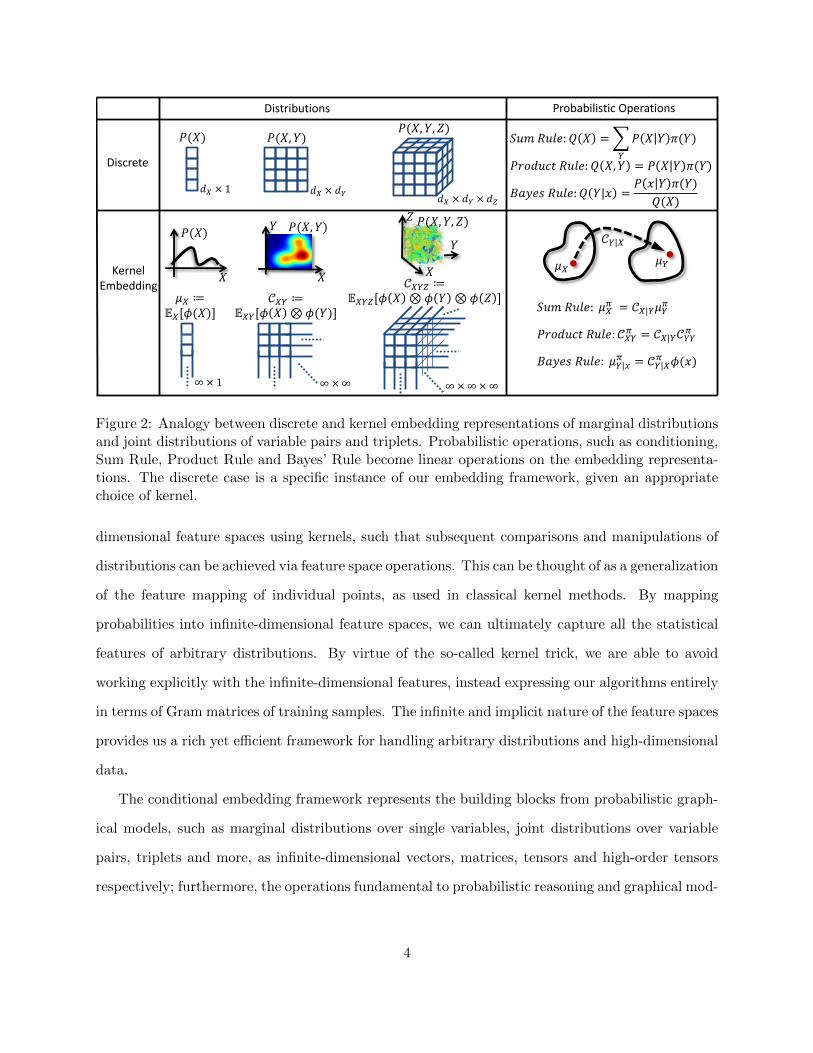
Figure 2: Analogy between discrete and kernel embedding representations of marginal distributionsand joint distributions of variable pairs and triplets. Probabilistic operations, such as conditioning,Sum Rule, Product Rule and Bayes’ Rule become linear operations on the embedding representa-tions. The discrete case is a specific instance of our embedding framework, given an appropriatechoice of kernel.

dimensional feature spaces using kernels, such that subsequent comparisons and manipulations of

distributions can be achieved via feature space operations. This can be thought of as a generalization

of the feature mapping of individual points, as used in classical kernel methods. By mapping

probabilities into infinite-dimensional feature spaces, we can ultimately capture all the statistical

features of arbitrary distributions. By virtue of the so-called kernel trick, we are able to avoid

working explicitly with the infinite-dimensional features, instead expressing our algorithms entirely

in terms of Gram matrices of training samples. The infinite and implicit nature of the feature spaces

provides us a rich yet efficient framework for handling arbitrary distributions and high-dimensional

data.

The conditional embedding framework represents the building blocks from probabilistic graph-

ical models, such as marginal distributions over single variables, joint distributions over variable

pairs, triplets and more, as infinite-dimensional vectors, matrices, tensors and high-order tensors

respectively; furthermore, the operations fundamental to probabilistic reasoning and graphical mod-

4

els, i.e., conditioning, Sum Rule, Product Rule and Bayes’ Rule, become linear transformations and

relations between the embeddings (see Figure 2 for the analogy between discrete probability tables

and kernel embeddings of distributions). We may combine these building blocks so as to reason

about interactions between a large collection of variables, even in the absence of parametric models.

The kernel conditional embedding framework has many advantages. First, it allows us to

model data with diverse statistical features without the need to make restrictive assumptions about

the type of distributions and relations. Second, it allows us to apply a large pool of linear and

multi-linear algebraic (tensor) tools to accomplish learning tasks in the presence of sophisticated

dependency structures, giving rise to methods for structure discovery, inference, parameter learning,

and latent feature extraction. Third, this framework can be applied not only to continuous variables,

but also can be generalized to variables which may take values on strings, graphs, groups, manifolds,

and other domains on which kernels may be defined. Fourth, the computation can be implemented

in practice by simple linear algebraic manipulation of kernel matrices.

We will mainly focus on two applications: the first being a belief propagation algorithm for

inference in nonparametric graphical models (i.e., estimating depth from still image features, re-

ported in [7]); and the second being a dynamical systems model (i.e., predicting camera movements

from video features, reported in [4]). In the first application, multi-modal components in graph-

ical models often make inference in these models intractable. Previous approaches using particle

filtering and ad hoc approximation with mixtures of Gaussians are slow and inaccurate. Using

kernel embeddings of conditional distributions, we are able to design a more accurate and efficient

algorithm for the problem. In the second application, both the observations and hidden states of

the hidden Markov model are complex high-dimensional variables, and it is not easy to capture

the structure of the data using parametric models. Kernel embeddings of conditional distributions

and kernel Bayes’ rule can be used to model such problems with better accuracy. Finally, there

exist many other recent applications of kernel embeddings of conditional distributions to signal pro-

cessing and machine learning problems, including Markov decision processes (MDP) [9], partially

observable MDPs (POMDPs) [10], hidden Markov models [6] and general latent variable graphical

models [8].

5

2 Kernel Embedding of Distributions

We begin by providing an overview of kernel embeddings of distributions, which are implicit map-

pings of distributions into potentially infinite dimensional feature spaces.1 We will see that the

definition is quite simple, yet the framework offers a number of advantages. For instance, it can

be used to design simpler and more effective statistics than alternatives for comparing continuous

valued multi-modal distributions, e.g., for the depth variable in Figure 1 application (a), and the

camera rotation variable in Figure 1 application (b).

We denote by X a random variable with domain Ω and distribution P (X), and refer to instan-

tiations of X by the lower case character, x. We will focus on continuous domains, and denote the

corresponding density by p(X). Similarly, we denote random variable Y with distribution P (Y )

and density p(Y ). For simplicity of notation, we assume that the domain of Y is also Ω, but the

methodology applies to the cases where X and Y have different domains.

A reproducing kernel Hilbert space (RKHS) F on Ω with a kernel k(x, x′) is a Hilbert space

of functions f : Ω 7→ R with inner product 〈·, ·〉F . Its element k(x, ·) satisfies the reproducing

property: 〈f(·), k(x, ·)〉F = f(x), and consequently, 〈k(x, ·), k(x′, ·)〉F = k(x, x′), meaning that we

can view the evaluation of a function f at any point x ∈ Ω as an inner product. Alternatively,

k(x, ·) can be viewed as an implicit feature map φ(x) where k(x, x′) = 〈φ(x), φ(x′)〉F .2 Popular

kernel functions on Rn include the polynomial kernel k(x, x′) = (〈x, x′〉+c)d and the Gaussian RBF

kernel k(x, x′) = exp(−σ ‖x− x′‖2). Kernel functions have also been defined on graphs, time series,

dynamical systems, images and other structured objects [13]. Thus the methodology presented

below can readily be generalized to a diverse range of data types as long as kernel functions are

defined for them.

1By “implicit”, we mean that we do not need to explicitly construct the feature spaces, and the actual computationsboil down to kernel matrix operations.

2For simplicity of notation, we use the same kernel for y, i.e., k(y, y′) = 〈φ(y), φ(y′)〉F

6

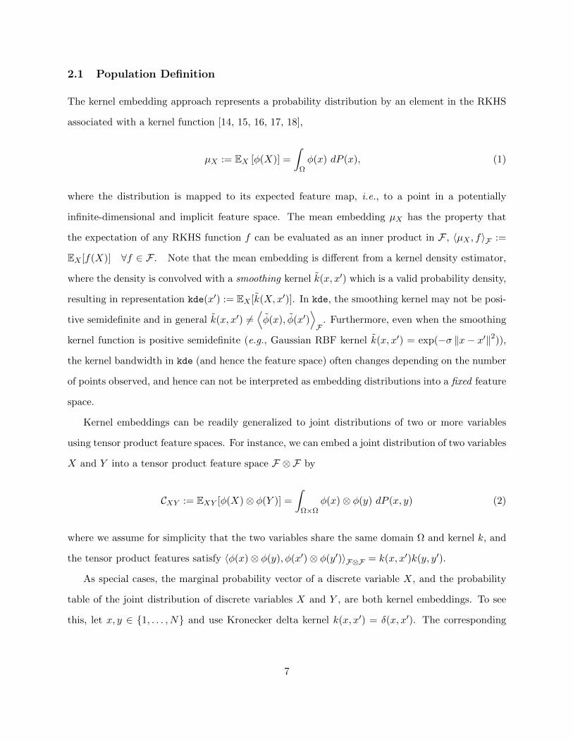
2.1 Population Definition

The kernel embedding approach represents a probability distribution by an element in the RKHS

associated with a kernel function [14, 15, 16, 17, 18],

µX := EX [φ(X)] =

∫Ωφ(x) dP (x), (1)

where the distribution is mapped to its expected feature map, i.e., to a point in a potentially

infinite-dimensional and implicit feature space. The mean embedding µX has the property that

the expectation of any RKHS function f can be evaluated as an inner product in F , 〈µX , f〉F :=

EX [f(X)] ∀f ∈ F . Note that the mean embedding is different from a kernel density estimator,

where the density is convolved with a smoothing kernel k(x, x′) which is a valid probability density,

resulting in representation kde(x′) := EX [k(X,x′)]. In kde, the smoothing kernel may not be posi-

tive semidefinite and in general k(x, x′) 6=⟨φ(x), φ(x′)

⟩F

. Furthermore, even when the smoothing

kernel function is positive semidefinite (e.g., Gaussian RBF kernel k(x, x′) = exp(−σ ‖x− x′‖2)),

the kernel bandwidth in kde (and hence the feature space) often changes depending on the number

of points observed, and hence can not be interpreted as embedding distributions into a fixed feature

space.

Kernel embeddings can be readily generalized to joint distributions of two or more variables

using tensor product feature spaces. For instance, we can embed a joint distribution of two variables

X and Y into a tensor product feature space F ⊗ F by

CXY := EXY [φ(X)⊗ φ(Y )] =

∫Ω×Ω

φ(x)⊗ φ(y) dP (x, y) (2)

where we assume for simplicity that the two variables share the same domain Ω and kernel k, and

the tensor product features satisfy 〈φ(x)⊗ φ(y), φ(x′)⊗ φ(y′)〉F⊗F = k(x, x′)k(y, y′).

As special cases, the marginal probability vector of a discrete variable X, and the probability

table of the joint distribution of discrete variables X and Y , are both kernel embeddings. To see

this, let x, y ∈ 1, . . . , N and use Kronecker delta kernel k(x, x′) = δ(x, x′). The corresponding

7

feature map φ(x) is then the standard basis of ex in RN . Then

P (x = 1)

...

P (x = N)

= EX [eX ] = µX ,

P (x = s, y = t)

= EXY [eX ⊗ eY ] = CXY . (3)

The joint embeddings can also be viewed as an uncentered cross-covariance operator CXY : F 7→

F by the standard equivalence between a tensor and a linear map. That is, given two functions

f, g ∈ F , their covariance can be computed by EXY [f(X)g(Y )] = 〈f, CXY g〉F , or equivalently

〈f ⊗ g, CXY 〉F⊗F , where in the former we view CXY as an operator while in the latter we view

it as an element in tensor product space. By analogy, CXX := EX [φ(X) ⊗ φ(X)] and C(XX)Y :=

EX [φ(X)⊗φ(X)⊗φ(Y )] can also be defined, the latter of which can be regarded as a linear operator

from F to F ⊗ F . It will be clear from the context whether we use CXY as an operator between

two spaces or as an element from a tensor product feature space.

Although the definition of embedding in (1) is simple, it turns out to have both rich representa-

tional power and a well-behaved empirical estimate. First, the mapping is injective for characteristic

kernels [17, 18]. That is, if two distributions, P (X) and Q(Y ), are different, they will be mapped

to two distinct points in the feature space. Many commonly used kernels are characteristic, such

as the Gaussian RBF kernel exp(−σ‖x − x′‖2) and Laplace kernel exp(−σ‖x − x′‖), which im-

plies that if we embed distributions using these kernels, the distance of the mappings in feature

space will give us an indication whether two distributions are identical or not. This intuition has

been exploited to design state-of-the-art two-sample tests [19] and independence tests [20]. For

the former case, the test statistic is the squared distance between the embeddings of P (Y ) and

Q(Y ), i.e., mmd(X,Y ) := ‖µX − µY ‖2F . For the latter case, the test statistic is the squared dis-

tance between the embeddings of a joint distribution P (X,Y ) and the product of its marginals

P (X)P (Y ), i.e., hsic(X,Y ) := ‖CXY − µX ⊗ µY ‖2F⊗F . Similarly, this statistic also has advan-

tages over the kde-based statistic. We will further discuss these tests in the next section, following

our introduction of finite sample estimates of the distribution embeddings and test statistics.

8

2.2 Finite Sample Kernel Estimator

While we rarely have access to the true underlying distribution, P (X), we can readily estimate

its embedding using a finite sample average. Given a sample DX = x1, . . . , xm of size m

drawn i.i.d. from P (X), the empirical kernel embedding is

µX =1

m

∑m

i=1φ(xi). (4)

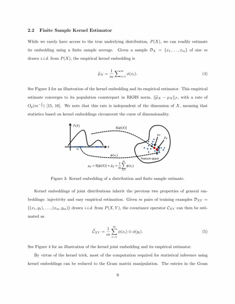
See Figure 3 for an illustration of the kernel embedding and its empirical estimator. This empirical

estimate converges to its population counterpart in RKHS norm, ‖µX − µX‖F , with a rate of

Op(m− 1

2 ) [15, 16]. We note that this rate is independent of the dimension of X, meaning that

statistics based on kernel embeddings circumvent the curse of dimensionality.

Feature space

𝜇𝑋 = 𝔼 𝜙 𝑋 ≈ 𝜇 𝑋 =1

𝑚 𝜙(𝑥𝑖)

𝑚

𝑖=1

𝜙 𝑥𝑖

𝔼 𝜙 𝑋 𝑃(𝑋)

𝑥𝑖 𝑋

𝜇𝑋 𝜇 𝑋

Figure 3: Kernel embedding of a distribution and finite sample estimate.

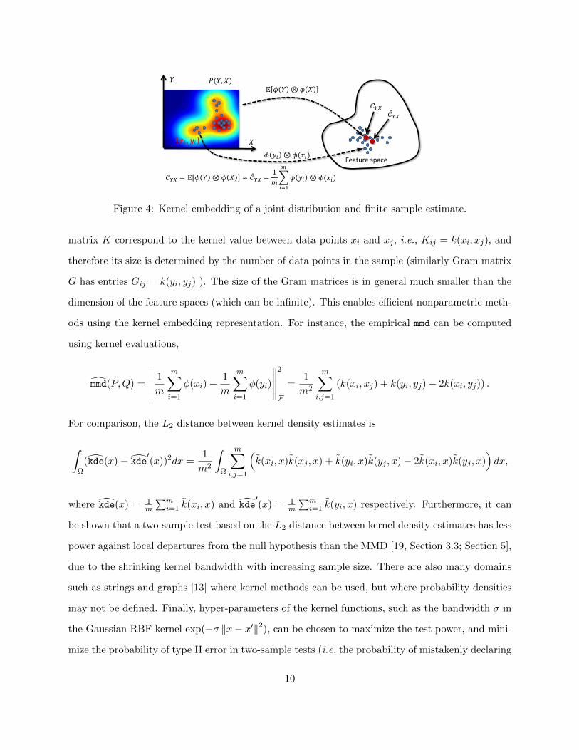
Kernel embeddings of joint distributions inherit the previous two properties of general em-

beddings: injectivity and easy empirical estimation. Given m pairs of training examples DXY =

(x1, y1), . . . , (xm, ym) drawn i.i.d. from P (X,Y ), the covariance operator CXY can then be esti-

mated as

CXY =1

m

m∑i=1

φ(xi)⊗ φ(yi). (5)

See Figure 4 for an illustration of the kernel joint embedding and its empirical estimator.

By virtue of the kernel trick, most of the computation required for statistical inference using

kernel embeddings can be reduced to the Gram matrix manipulation. The entries in the Gram

9

Feature space

𝒞𝑌𝑋 = 𝔼 𝜙 𝑌 ⊗ 𝜙 𝑋 ≈ 𝒞 𝑌𝑋 =1

𝑚 𝜙 𝑦𝑖 ⊗ 𝜙(𝑥𝑖)

𝑚

𝑖=1

𝔼 𝜙 𝑌 ⊗ 𝜙 𝑋

𝜙 𝑦𝑖 ⊗ 𝜙(𝑥𝑖)

𝑃(𝑌, 𝑋) 𝑌

𝑋

𝒞𝑌𝑋 𝒞 𝑌𝑋

Figure 4: Kernel embedding of a joint distribution and finite sample estimate.

matrix K correspond to the kernel value between data points xi and xj , i.e., Kij = k(xi, xj), and

therefore its size is determined by the number of data points in the sample (similarly Gram matrix

G has entries Gij = k(yi, yj) ). The size of the Gram matrices is in general much smaller than the

dimension of the feature spaces (which can be infinite). This enables efficient nonparametric meth-

ods using the kernel embedding representation. For instance, the empirical mmd can be computed

using kernel evaluations,

mmd(P,Q) =

∥∥∥∥∥ 1

m

m∑i=1

φ(xi)−1

m

m∑i=1

φ(yi)

∥∥∥∥∥2

F

=1

m2

m∑i,j=1

(k(xi, xj) + k(yi, yj)− 2k(xi, yj)) .

For comparison, the L2 distance between kernel density estimates is

∫Ω

(kde(x)− kde′(x))2dx =

1

m2

∫Ω

m∑i,j=1

(k(xi, x)k(xj , x) + k(yi, x)k(yj , x)− 2k(xi, x)k(yj , x)

)dx,

where kde(x) = 1m

∑mi=1 k(xi, x) and kde

′(x) = 1

m

∑mi=1 k(yi, x) respectively. Furthermore, it can

be shown that a two-sample test based on the L2 distance between kernel density estimates has less

power against local departures from the null hypothesis than the MMD [19, Section 3.3; Section 5],

due to the shrinking kernel bandwidth with increasing sample size. There are also many domains

such as strings and graphs [13] where kernel methods can be used, but where probability densities

may not be defined. Finally, hyper-parameters of the kernel functions, such as the bandwidth σ in

the Gaussian RBF kernel exp(−σ ‖x− x′‖2), can be chosen to maximize the test power, and mini-

mize the probability of type II error in two-sample tests (i.e. the probability of mistakenly declaring

10

P and Q are the same when they are in fact different) [21]. MMD and other distances between

samples of points were also suggested in [22], although the injectivity of the map of probability

measures to feature space, and the question of whether a metric was induced on probabilities, were

not addressed.

If the sample size is large, the computation in kernel embedding methods may be expensive.

In this case, a popular solution is to use a low-rank approximation of the Gram matrix, such

as incomplete Cholesky factorization [23], which is known to work very effectively in reducing

computational cost of kernel methods, while maintaining the approximation accuracy.

3 Kernel Embeddings of Conditional Distributions

While kernel embeddings of distributions provide a powerful framework for dealing with a number

of challenging high-dimensional nonparametric problems, there remain many issues to be addressed

in using these embeddings for inference. For instance, in Figure 1 application (a) and (b), there are

many random variables interlinked via graphical models, and a simple embedding of distribution

is not able to exploit the knowledge of these conditional independence relations. Furthermore, a

key inference task in graphical models is to compute the posterior distribution of some hidden

variables (e.g., depth variable in application (a) and camera orientation in application (b)) given

some observed evidence (e.g., image pixel values in application (a) and video frames in application

(b)). Such conditional operation is also missing in kernel embedding of distributions. Thus, in

this section we will present a kernel nonparametric counterpart for conditional distributions, which

will allows us to take into account conditional independence relations in graphical models, and

subsequently provide a unified kernel framework for the Sum Rule, Product Rule and Bayes’ Rule,

essential for probabilistic reasoning in graphical models.

11

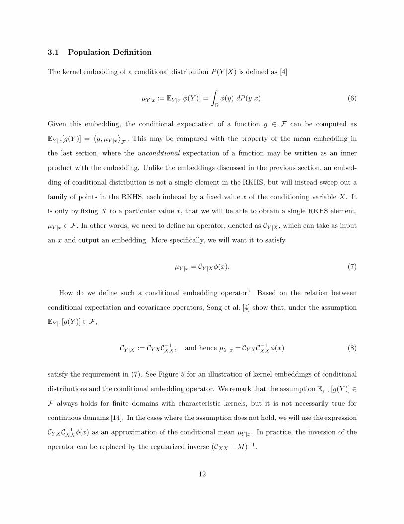
3.1 Population Definition

The kernel embedding of a conditional distribution P (Y |X) is defined as [4]

µY |x := EY |x[φ(Y )] =

∫Ωφ(y) dP (y|x). (6)

Given this embedding, the conditional expectation of a function g ∈ F can be computed as

EY |x[g(Y )] =⟨g, µY |x

⟩F . This may be compared with the property of the mean embedding in

the last section, where the unconditional expectation of a function may be written as an inner

product with the embedding. Unlike the embeddings discussed in the previous section, an embed-

ding of conditional distribution is not a single element in the RKHS, but will instead sweep out a

family of points in the RKHS, each indexed by a fixed value x of the conditioning variable X. It

is only by fixing X to a particular value x, that we will be able to obtain a single RKHS element,

µY |x ∈ F . In other words, we need to define an operator, denoted as CY |X , which can take as input

an x and output an embedding. More specifically, we will want it to satisfy

µY |x = CY |Xφ(x). (7)

How do we define such a conditional embedding operator? Based on the relation between

conditional expectation and covariance operators, Song et al. [4] show that, under the assumption

EY |· [g(Y )] ∈ F ,

CY |X := CY XC−1XX , and hence µY |x = CY XC−1

XXφ(x) (8)

satisfy the requirement in (7). See Figure 5 for an illustration of kernel embeddings of conditional

distributions and the conditional embedding operator. We remark that the assumption EY |· [g(Y )] ∈

F always holds for finite domains with characteristic kernels, but it is not necessarily true for

continuous domains [14]. In the cases where the assumption does not hold, we will use the expression

CY XC−1XXφ(x) as an approximation of the conditional mean µY |x. In practice, the inversion of the

operator can be replaced by the regularized inverse (CXX + λI)−1.

12

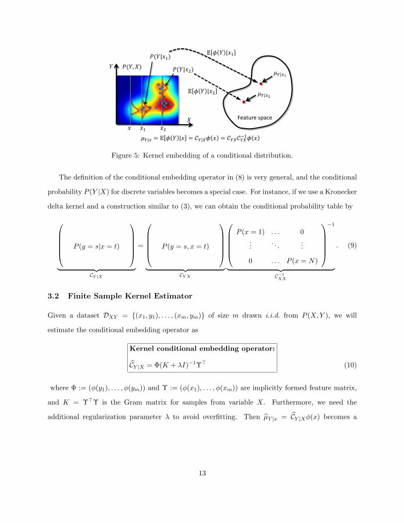
Feature space

𝔼 𝜙 𝑌 |𝑥1

𝑃(𝑌, 𝑋) 𝑌

𝔼 𝜙 𝑌 |𝑥2

𝑃(𝑌|𝑥1)

𝑃(𝑌|𝑥2) 𝜇𝑌|𝑥1

𝜇𝑌|𝑥2

𝑋

𝑥 𝑥1 𝑥2

𝜇𝑌|𝑥 = 𝔼 𝜙 𝑌 |𝑥 = 𝒞𝑌|𝑋𝜙 𝑥 = 𝒞𝑌𝑋𝒞𝑌𝑋−1𝜙 𝑥

Figure 5: Kernel embedding of a conditional distribution.

The definition of the conditional embedding operator in (8) is very general, and the conditional

probability P (Y |X) for discrete variables becomes a special case. For instance, if we use a Kronecker

delta kernel and a construction similar to (3), we can obtain the conditional probability table by

P (y = s|x = t)

︸ ︷︷ ︸

CY |X

=

P (y = s, x = t)

︸ ︷︷ ︸

CYX

P (x = 1) . . . 0

.... . .

...

0 . . . P (x = N)

−1

︸ ︷︷ ︸C−1XX

. (9)

3.2 Finite Sample Kernel Estimator

Given a dataset DXY = (x1, y1), . . . , (xm, ym) of size m drawn i.i.d. from P (X,Y ), we will

estimate the conditional embedding operator as

Kernel conditional embedding operator:

CY |X = Φ(K + λI)−1Υ> (10)

where Φ := (φ(y1), . . . , φ(ym)) and Υ := (φ(x1), . . . , φ(xm)) are implicitly formed feature matrix,

and K = Υ>Υ is the Gram matrix for samples from variable X. Furthermore, we need the

additional regularization parameter λ to avoid overfitting. Then µY |x = CY |Xφ(x) becomes a

13

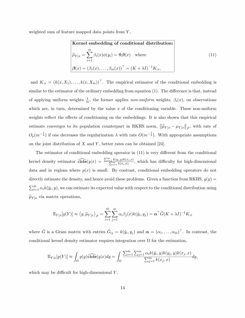
weighted sum of feature mapped data points from Y ,

Kernel embedding of conditional distribution:

µY |x =

m∑i=1

βi(x)φ(yi) = Φβ(x) where

β(x) = (β1(x), . . . , βm(x))> = (K + λI)−1K:x,

(11)

and K:x = (k(x,X1), . . . , k(x,Xm))>. The empirical estimator of the conditional embedding is

similar to the estimator of the ordinary embedding from equation (1). The difference is that, instead

of applying uniform weights 1m , the former applies non-uniform weights, βi(x), on observations

which are, in turn, determined by the value x of the conditioning variable. These non-uniform

weights reflect the effects of conditioning on the embeddings. It is also shown that this empirical

estimate converges to its population counterpart in RKHS norm,∥∥µY |x − µY |x∥∥F , with rate of

Op(m− 1

4 ) if one decreases the regularization λ with rate O(m−12 ). With appropriate assumptions

on the joint distribution of X and Y , better rates can be obtained [24].

The estimator of conditional embedding operator in (11) is very different from the conditional

kernel density estimator ckde(y|x) =∑mi=1 k(yi,y)k(xi,x)∑m

i=1 k(xi,x), which has difficulty for high-dimensional

data and in regions where p(x) is small. By contrast, conditional embedding operators do not

directly estimate the density, and hence avoid these problems. Given a function from RKHS, g(y) =∑mi=1 αik(yi, y), we can estimate its expected value with respect to the conditional distribution using

µY |x via matrix operations,

EY |x[g(Y )] ≈⟨g, µY |x

⟩F =

m∑i=1

m∑j=1

αiβj(x)k(yi, yj) = α>G(K + λI)−1K:x

where G is a Gram matrix with entries Gij = k(yi, yj) and α = (α1, . . . , αm)>. In contrast, the

conditional kernel density estimator requires integration over Ω for the estimation,

EY |x[g(Y )] ≈∫

Ωg(y)ckde(y|x)dy =

∫Ω

∑mi=1

∑mj=1 αik(yi, y)k(yj , y)k(xj , x)∑m

j=1 k(xj , x)dy,

which may be difficult for high-dimensional Y .

14

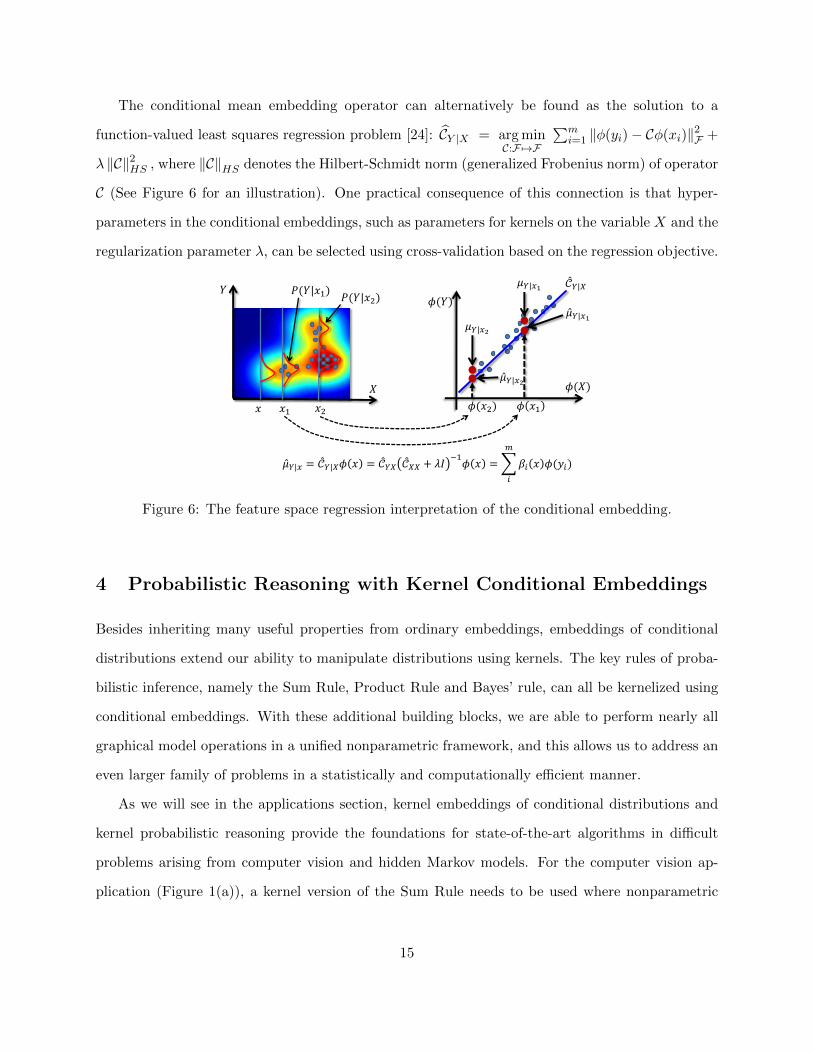
The conditional mean embedding operator can alternatively be found as the solution to a

function-valued least squares regression problem [24]: CY |X = arg minC:F7→F

∑mi=1 ‖φ(yi)− Cφ(xi)‖2F +

λ ‖C‖2HS , where ‖C‖HS denotes the Hilbert-Schmidt norm (generalized Frobenius norm) of operator

C (See Figure 6 for an illustration). One practical consequence of this connection is that hyper-

parameters in the conditional embeddings, such as parameters for kernels on the variable X and the

regularization parameter λ, can be selected using cross-validation based on the regression objective.

𝑌 𝑃(𝑌|𝑥2)

𝜇𝑌|𝑥1

𝑋

𝑥 𝑥2 𝜙(𝑥2) 𝜙 𝑥1

𝜇𝑌|𝑥2

𝜇 𝑌|𝑥1

𝜇 𝑌|𝑥2

𝒞 𝑌|𝑋

𝜇 𝑌|𝑥 = 𝒞 𝑌|𝑋𝜙 𝑥 = 𝒞 𝑌𝑋 𝒞 𝑋𝑋 + 𝜆𝐼−1

𝜙 𝑥 = 𝛽𝑖 𝑥 𝜙(𝑦𝑖)

𝑚

𝑖

𝑃(𝑌|𝑥1)

𝑥1

𝜙(𝑋)

𝜙(𝑌)

Figure 6: The feature space regression interpretation of the conditional embedding.

4 Probabilistic Reasoning with Kernel Conditional Embeddings

Besides inheriting many useful properties from ordinary embeddings, embeddings of conditional

distributions extend our ability to manipulate distributions using kernels. The key rules of proba-

bilistic inference, namely the Sum Rule, Product Rule and Bayes’ rule, can all be kernelized using

conditional embeddings. With these additional building blocks, we are able to perform nearly all

graphical model operations in a unified nonparametric framework, and this allows us to address an

even larger family of problems in a statistically and computationally efficient manner.

As we will see in the applications section, kernel embeddings of conditional distributions and

kernel probabilistic reasoning provide the foundations for state-of-the-art algorithms in difficult

problems arising from computer vision and hidden Markov models. For the computer vision ap-

plication (Figure 1(a)), a kernel version of the Sum Rule needs to be used where nonparametric

15

multi-modal incoming messages are aggregated to produce a nonparametric outgoing message. For

the hidden Markov model application (Figure 1(b)), a kernel Bayes rule needs to be used where

nonparametric posterior distributions of the hidden states are maintained given video observations.

In the following, we will denote a joint distribution over X and Y by P (X,Y ), with marginal dis-

tributions P (X) =∫

Ω P (X, dy) and P (Y ) =∫

Ω P (dx, Y ), and conditional distribution P (Y |X) =

P (X,Y )P (X) . The conditional embedding operator associated with P (Y |X) is CY |X ; similarly, P (X|Y ) =

P (X,Y )P (Y ) is associated with CX|Y . Furthermore, we will denote a prior distribution over Y by π(Y ).

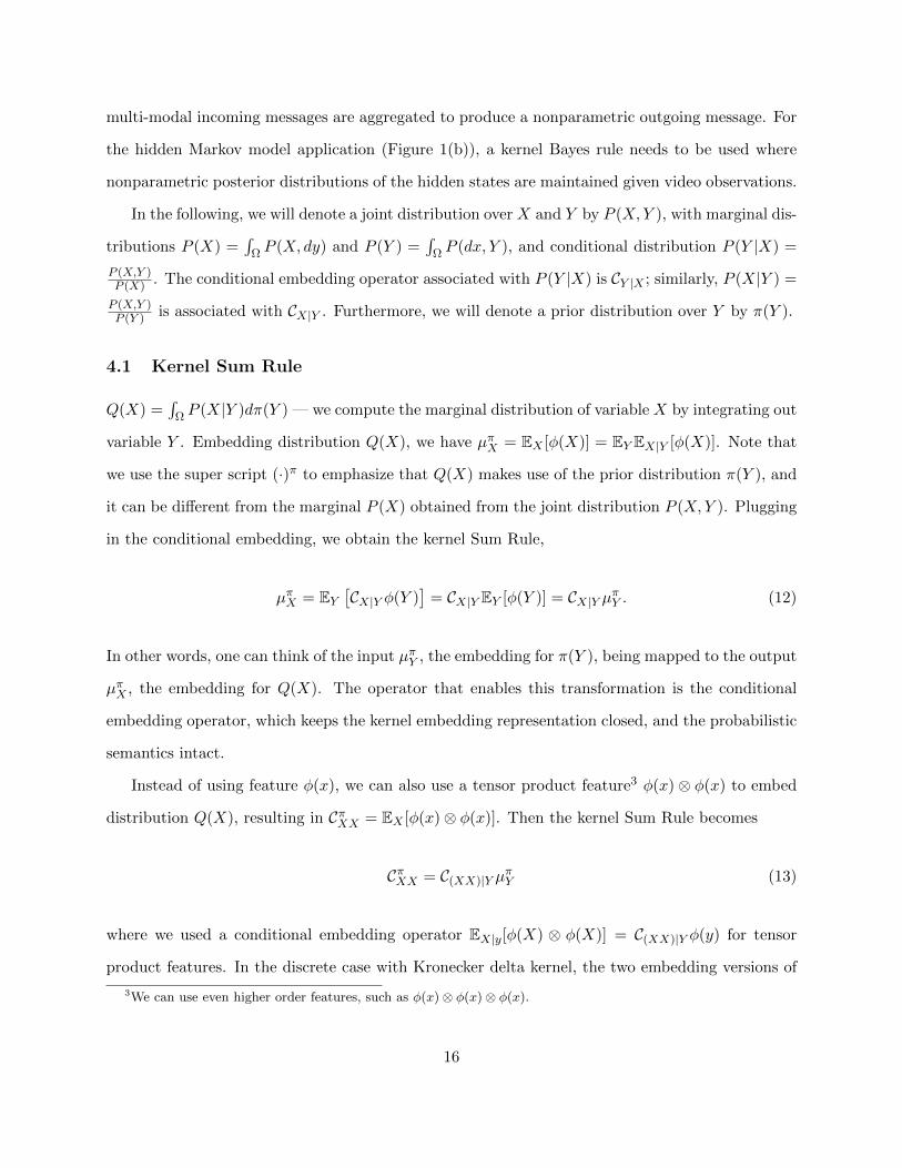
4.1 Kernel Sum Rule

Q(X) =∫

Ω P (X|Y )dπ(Y ) — we compute the marginal distribution of variable X by integrating out

variable Y . Embedding distribution Q(X), we have µπX = EX [φ(X)] = EY EX|Y [φ(X)]. Note that

we use the super script (·)π to emphasize that Q(X) makes use of the prior distribution π(Y ), and

it can be different from the marginal P (X) obtained from the joint distribution P (X,Y ). Plugging

in the conditional embedding, we obtain the kernel Sum Rule,

µπX = EY[CX|Y φ(Y )

]= CX|Y EY [φ(Y )] = CX|Y µπY . (12)

In other words, one can think of the input µπY , the embedding for π(Y ), being mapped to the output

µπX , the embedding for Q(X). The operator that enables this transformation is the conditional

embedding operator, which keeps the kernel embedding representation closed, and the probabilistic

semantics intact.

Instead of using feature φ(x), we can also use a tensor product feature3 φ(x)⊗ φ(x) to embed

distribution Q(X), resulting in CπXX = EX [φ(x)⊗ φ(x)]. Then the kernel Sum Rule becomes

CπXX = C(XX)|Y µπY (13)

where we used a conditional embedding operator EX|y[φ(X) ⊗ φ(X)] = C(XX)|Y φ(y) for tensor

product features. In the discrete case with Kronecker delta kernel, the two embedding versions of

3We can use even higher order features, such as φ(x)⊗ φ(x)⊗ φ(x).

16

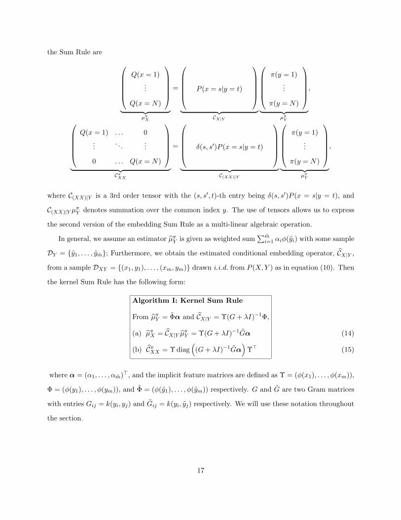
the Sum Rule are Q(x = 1)

...

Q(x = N)

︸ ︷︷ ︸

µπX

=

P (x = s|y = t)

︸ ︷︷ ︸

CX|Y

π(y = 1)

...

π(y = N)

︸ ︷︷ ︸

µπY

,

Q(x = 1) . . . 0

.... . .

...

0 . . . Q(x = N)

︸ ︷︷ ︸

CπXX

=

δ(s, s′)P (x = s|y = t)

︸ ︷︷ ︸

C(XX)|Y

π(y = 1)

...

π(y = N)

︸ ︷︷ ︸

µπY

,

where C(XX)|Y is a 3rd order tensor with the (s, s′, t)-th entry being δ(s, s′)P (x = s|y = t), and

C(XX)|Y µπY denotes summation over the common index y. The use of tensors allows us to express

the second version of the embedding Sum Rule as a multi-linear algebraic operation.

In general, we assume an estimator µπY is given as weighted sum∑m

i=1 αiφ(yi) with some sample

DY = y1, . . . , ym; Furthermore, we obtain the estimated conditional embedding operator, CX|Y ,

from a sample DXY = (x1, y1), . . . , (xm, ym) drawn i.i.d. from P (X,Y ) as in equation (10). Then

the kernel Sum Rule has the following form:

Algorithm I: Kernel Sum Rule

From µπY = Φα and CX|Y = Υ(G+ λI)−1Φ,

(a) µπX = CX|Y µπY = Υ(G+ λI)−1Gα

(b) CπXX = Υ diag(

(G+ λI)−1Gα)

Υ>

(14)

(15)

where α = (α1, . . . , αm)>, and the implicit feature matrices are defined as Υ = (φ(x1), . . . , φ(xm)),

Φ = (φ(y1), . . . , φ(ym)), and Φ = (φ(y1), . . . , φ(ym)) respectively. G and G are two Gram matrices

with entries Gij = k(yi, yj) and Gij = k(yi, yj) respectively. We will use these notation throughout

the section.

17

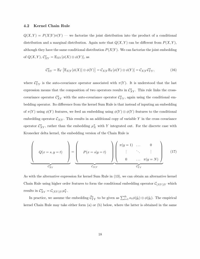
4.2 Kernel Chain Rule

Q(X,Y ) = P (X|Y )π(Y ) — we factorize the joint distribution into the product of a conditional

distribution and a marginal distribution. Again note that Q(X,Y ) can be different from P (X,Y ),

although they have the same conditional distribution P (X|Y ). We can factorize the joint embedding

of Q(X,Y ), CπXY = EXY [φ(X)⊗ φ(Y )], as

CπXY = EY[EX|Y [φ(X)]⊗ φ(Y )

]= CX|Y EY [φ(Y )⊗ φ(Y )] = CX|Y CπY Y , (16)

where CπY Y is the auto-covariance operator associated with π(Y ). It is understood that the last

expression means that the composition of two operators results in CπXY . This rule links the cross-

covariance operator CπXY with the auto-covariance operator CπY Y , again using the conditional em-

bedding operator. Its difference from the kernel Sum Rule is that instead of inputing an embedding

of π(Y ) using φ(Y ) features, we feed an embedding using φ(Y )⊗ φ(Y ) features to the conditional

embedding operator CX|Y . This results in an additional copy of variable Y in the cross covariance

operator CπXY , rather than the embedding µπX with Y integrated out. For the discrete case with

Kronecker delta kernel, the embedding version of the Chain Rule is

Q(x = s, y = t)

︸ ︷︷ ︸

CπXY

=

P (x = s|y = t)

︸ ︷︷ ︸

CX|Y

π(y = 1) . . . 0

.... . .

...

0 . . . π(y = N)

︸ ︷︷ ︸

CπY Y

(17)

As with the alternative expression for kernel Sum Rule in (13), we can obtain an alternative kernel

Chain Rule using higher order features to form the conditional embedding operator C(XY )|Y which

results in CπXY = C(XY )|Y µπY .

In practice, we assume the embedding CπY Y to be given as∑m

i=1 αiφ(yi)⊗ φ(yi). The empirical

kernel Chain Rule may take either form (a) or (b) below, where the latter is obtained in the same

18

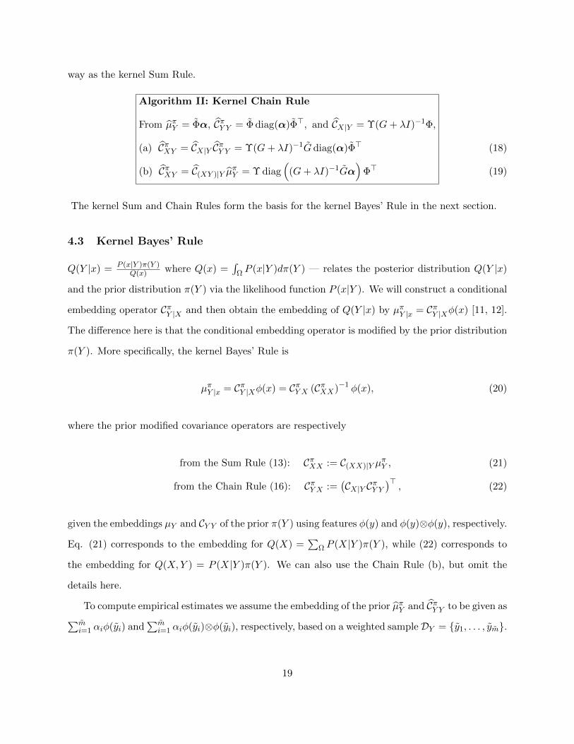
way as the kernel Sum Rule.

Algorithm II: Kernel Chain Rule

From µπY = Φα, CπY Y = Φ diag(α)Φ>, and CX|Y = Υ(G+ λI)−1Φ,

(a) CπXY = CX|Y CπY Y = Υ(G+ λI)−1G diag(α)Φ>

(b) CπXY = C(XY )|Y µπY = Υ diag

((G+ λI)−1Gα

)Φ>

(18)

(19)

The kernel Sum and Chain Rules form the basis for the kernel Bayes’ Rule in the next section.

4.3 Kernel Bayes’ Rule

Q(Y |x) = P (x|Y )π(Y )Q(x) where Q(x) =

∫Ω P (x|Y )dπ(Y ) — relates the posterior distribution Q(Y |x)

and the prior distribution π(Y ) via the likelihood function P (x|Y ). We will construct a conditional

embedding operator CπY |X and then obtain the embedding of Q(Y |x) by µπY |x = CπY |Xφ(x) [11, 12].

The difference here is that the conditional embedding operator is modified by the prior distribution

π(Y ). More specifically, the kernel Bayes’ Rule is

µπY |x = CπY |Xφ(x) = CπY X (CπXX)−1 φ(x), (20)

where the prior modified covariance operators are respectively

from the Sum Rule (13): CπXX := C(XX)|Y µπY , (21)

from the Chain Rule (16): CπY X :=(CX|Y CπY Y

)>, (22)

given the embeddings µY and CY Y of the prior π(Y ) using features φ(y) and φ(y)⊗φ(y), respectively.

Eq. (21) corresponds to the embedding for Q(X) =∑

Ω P (X|Y )π(Y ), while (22) corresponds to

the embedding for Q(X,Y ) = P (X|Y )π(Y ). We can also use the Chain Rule (b), but omit the

details here.

To compute empirical estimates we assume the embedding of the prior µπY and CπY Y to be given as∑mi=1 αiφ(yi) and

∑mi=1 αiφ(yi)⊗φ(yi), respectively, based on a weighted sample DY = y1, . . . , ym.

19

Then using kernel Sum Rule and kernel Chain Rule, we obtain the kernel Bayes’ Rule,

Algorithm III: Kernel Bayes’ Rule

Let: Λ := (G+ λI)−1Gdiag(α), D = diag((G+ λI)−1Gα)

From kernel Sum Rule: CπXX = ΥDΥ>

From kernel Chain Rule: (a) CπY X = ΦΛ>Υ>, (b) CπY X = ΦDΥ>

(a) µY |x = CπY X((CπXX)2 + λI)−1CπXXφ(x) = ΦΛ>((DK)2 + λI)−1KDK:x

(b) µY |x = CπY X((CπXX)2 + λI)−1CπXXφ(x) = ΦDK((DK)2 + λI)−1DK:x

(23)

(24)

In the kernel Bayes’ rule, there are two regularization parameters λ and λ: one is used in estimating

the prior modified covariance operators, CπXX and CπY X , and the other is used in estimating the final

conditional embedding operator, CπY |X = CπY X((CπXX)2 + λI)−1CπXX . Since the estimator D may

not be positive definite, the latter regularization parameter λ is used on the square of CπXX . We

can see that the embedding of the posterior distribution has a form of∑m

i=1 βi(x)φ(yi), where

β(x) = Λ>((DK)2 + λI)−1KDK:x or β = DK((DK)2 + λI)−1DK:x.

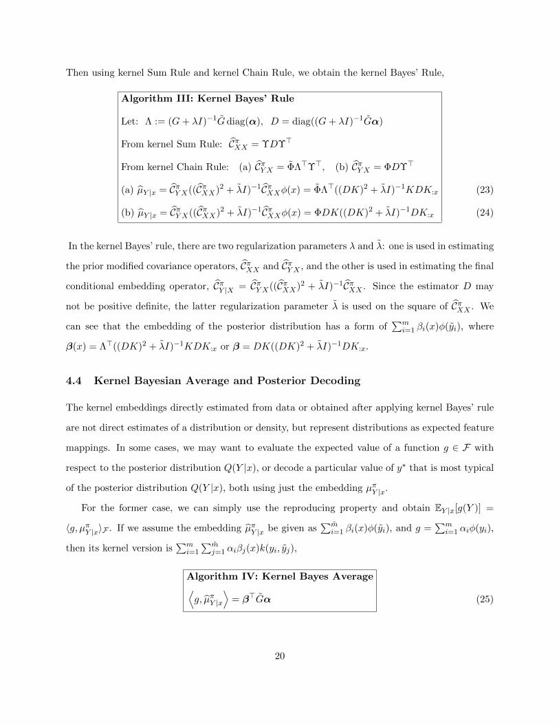
4.4 Kernel Bayesian Average and Posterior Decoding

The kernel embeddings directly estimated from data or obtained after applying kernel Bayes’ rule

are not direct estimates of a distribution or density, but represent distributions as expected feature

mappings. In some cases, we may want to evaluate the expected value of a function g ∈ F with

respect to the posterior distribution Q(Y |x), or decode a particular value of y∗ that is most typical

of the posterior distribution Q(Y |x), both using just the embedding µπY |x.

For the former case, we can simply use the reproducing property and obtain EY |x[g(Y )] =

〈g, µπY |x〉F . If we assume the embedding µπY |x be given as∑m

i=1 βi(x)φ(yi), and g =∑m

i=1 αiφ(yi),

then its kernel version is∑m

i=1

∑mj=1 αiβj(x)k(yi, yj),

Algorithm IV: Kernel Bayes Average⟨g, µπY |x

⟩= β>Gα (25)

20

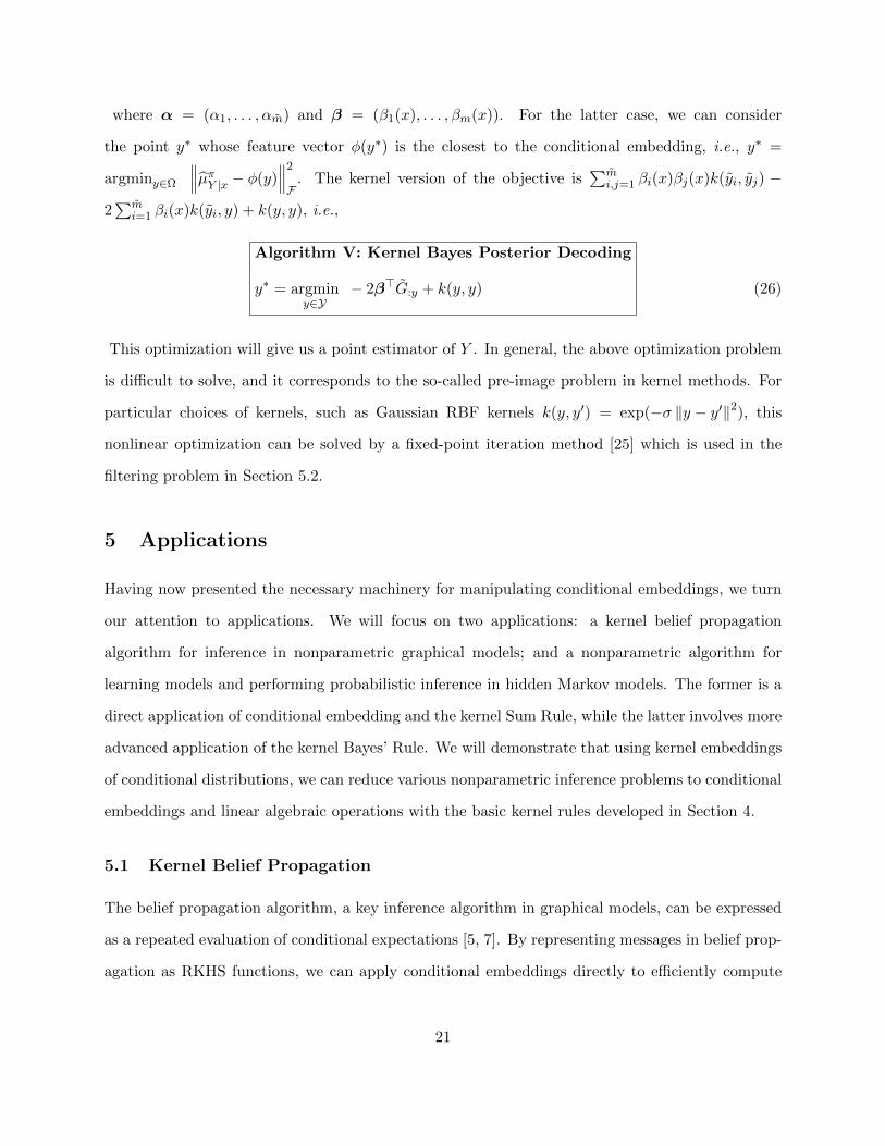
where α = (α1, . . . , αm) and β = (β1(x), . . . , βm(x)). For the latter case, we can consider

the point y∗ whose feature vector φ(y∗) is the closest to the conditional embedding, i.e., y∗ =

argminy∈Ω

∥∥∥µπY |x − φ(y)∥∥∥2

F. The kernel version of the objective is

∑mi,j=1 βi(x)βj(x)k(yi, yj) −

2∑m

i=1 βi(x)k(yi, y) + k(y, y), i.e.,

Algorithm V: Kernel Bayes Posterior Decoding

y∗ = argminy∈Y

− 2β>G:y + k(y, y) (26)

This optimization will give us a point estimator of Y . In general, the above optimization problem

is difficult to solve, and it corresponds to the so-called pre-image problem in kernel methods. For

particular choices of kernels, such as Gaussian RBF kernels k(y, y′) = exp(−σ ‖y − y′‖2), this

nonlinear optimization can be solved by a fixed-point iteration method [25] which is used in the

filtering problem in Section 5.2.

5 Applications

Having now presented the necessary machinery for manipulating conditional embeddings, we turn

our attention to applications. We will focus on two applications: a kernel belief propagation

algorithm for inference in nonparametric graphical models; and a nonparametric algorithm for

learning models and performing probabilistic inference in hidden Markov models. The former is a

direct application of conditional embedding and the kernel Sum Rule, while the latter involves more

advanced application of the kernel Bayes’ Rule. We will demonstrate that using kernel embeddings

of conditional distributions, we can reduce various nonparametric inference problems to conditional

embeddings and linear algebraic operations with the basic kernel rules developed in Section 4.

5.1 Kernel Belief Propagation

The belief propagation algorithm, a key inference algorithm in graphical models, can be expressed

as a repeated evaluation of conditional expectations [5, 7]. By representing messages in belief prop-

agation as RKHS functions, we can apply conditional embeddings directly to efficiently compute

21

message updates. This observation allows us to develop a nonparametric belief propagation algo-

rithm which achieves better accuracy in the problem of predicting depth from image features. See

Figure 1(a) for an illustration.

5.1.1 Problem Formulation

We begin with a short introduction to pairwise Markov random fields (MRFs) and the belief

propagation algorithm. A pairwise Markov random field (MRF) is defined on an undirected graph

G := (V, E) with nodes V := 1, . . . , n connected by edges in E . Each node s ∈ V is associated

with a random variable Xs on the domain X (we assume a common domain for ease of notation,

but in practice the domains can be different), and Γs := t|(s, t) ∈ E is the set of neighbors of node

s with size ds := |Γs|. In a pairwise MRF, the joint density of the variables X := X1, . . . , X|V|

is assumed to factorize according to a model p(X) = 1Z

∏(s,t)∈E Ψst(Xs, Xt)

∏s∈V Ψs(Xs), where

Ψs(Xs) and Ψst(Xs, Xt) are node and edge potentials respectively, and Z is the partition function

that normalizes the distribution.

The inference problem in an MRF is defined as calculating the marginal densities p(Xs) for nodes

s ∈ V. Belief Propagation (BP) is an iterative algorithm for performing approximate inference in

MRFs [1]. BP represents intermediate results of marginalization steps as messages passed between

adjacent nodes: a message mts from t to s is calculated based on messages mut from all neighboring

nodes u of t besides s, i.e., [7]

mts(xs) =

∫Ωp?(Xt|xs)

∏u\s

mut(Xt) dXt = EXt|xs

[∏u\s

mut(Xt)

]. (27)

Note that we use∏u\s to denote

∏u∈Γt\s, where it is understood that the indexes range over

all neighbors u of t except s. This notation also applies to operations other than the product.

Furthermore, p?(Xt|xs) denotes the true conditional distribution of Xt. Using similar reasoning, the

node belief, an estimate of p(Xs), takes the form B(Xs) ∝ p?(Xs)∏t∈Γs

m?ts(Xs) on convergence

of BP, i.e., the message converges to m?ts(Xs). Our goal is to develop a nonparametric belief

propagation algorithm, where the potentials are nonparametric functions learned from data, such

that multi-modal and other non-Gaussian statistical features can be captured. Most crucially, these

22

potentials must be represented in such a way that the message update in (27) is computationally

tractable.

5.1.2 Kernel Algorithm

We will assume that a messagemut(xt) is in the reproducing kernel Hilbert space (RKHS), i.e.,mut(xt) =

〈mut, φ(xt)〉. In an evidence node Xu where the evidence is fixed to xu, its outgoing message is

simply the likelihood function p(xu|xt), and we can estimate it as a RKHS function. That is given

m samples, mut(·) = p(xu|·) =∑m

i=1 βiutk(xit, ·) [5]. As we will see, the advantage of this assump-

tion is that the update procedure using kernel conditional embedding can be expressed as a linear

operation in the RKHS, and results in new messages that are likewise RKHS functions.

We begin by defining a tensor product reproducing kernel Hilbert space H := ⊗dt−1F , under

which the product of incoming messages can be written as a single inner product. For a node t with

degree dt = |Γt|, the product of incoming messages mut from all neighbors except s becomes an

inner product in H,∏u\smut(Xt) =

∏u\s 〈mut, φ(Xt)〉F =

⟨⊗u\smut, ξ(Xt)

⟩H, where ξ(Xt) :=⊗

u\s φ(Xt). The message update (27) becomes mts(xs) =⟨⊗

u\smut, EXt|xs [ξ(Xt)]⟩H. We can

define the conditional embedding operator for the tensor product of features, such that CX⊗t |Xs :

F → H satisfies

µX⊗t |xs:= EXt|xs [ξ(Xt)] = CX⊗t |Xsφ(xs). (28)

As in the single variable case, CX⊗t |Xs is defined in terms of a covariance operator CX⊗t Xs :=

EXtXs [ξ(Xt)⊗ φ(Xs)] in the tensor space, and the operator CXsXs . The operator CX⊗t |Xs takes the

feature map φ(xs) of the point on which we condition, and outputs the conditional expectation of

the tensor product feature ξ(Xt). Consequently, we can express the message update as a linear

operation, but in a tensor product feature space,

mts(xs) =

⟨⊗u\s

mut, CX⊗t |Xsφ(xs)

⟩H. (29)

The belief at a specific node s can be computed as B(Xs) = p?(Xs)∏u∈Γs

mus(Xs) where the true

23

marginal p(Xr) can be estimated using a kernel density estimator.

Now given m samples, and applying the kernel estimator for conditional embedding operator

in (10), we can obtain a kernel expression for the message update in (29). Let the incoming message

be mut(·) =∑m

i=1 βiutk(xit, ·), then

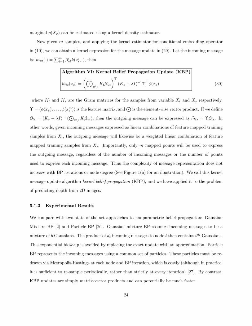
Algorithm VI: Kernel Belief Propagation Update (KBP)

mts(xs) =

(⊙u\s

Ktβut

)>(Ks + λI)−1Υ>φ(xs) (30)

where Kt and Ks are the Gram matrices for the samples from variable Xt and Xs respectively,

Υ = (φ(x1s), . . . , φ(xms )) is the feature matrix, and

⊙is the element-wise vector product. If we define

βts = (Ks + λI)−1(⊙

u\sKβut), then the outgoing message can be expressed as mts = Υβts. In

other words, given incoming messages expressed as linear combinations of feature mapped training

samples from Xt, the outgoing message will likewise be a weighted linear combination of feature

mapped training samples from Xs. Importantly, only m mapped points will be used to express

the outgoing message, regardless of the number of incoming messages or the number of points

used to express each incoming message. Thus the complexity of message representation does not

increase with BP iterations or node degree (See Figure 1(a) for an illustration). We call this kernel

message update algorithm kernel belief propagation (KBP), and we have applied it to the problem

of predicting depth from 2D images.

5.1.3 Experimental Results

We compare with two state-of-the-art approaches to nonparametric belief propagation: Gaussian

Mixture BP [2] and Particle BP [26]. Gaussian mixture BP assumes incoming messages to be a

mixture of b Gaussians. The product of dt incoming messages to node t then contains bdt Gaussians.

This exponential blow-up is avoided by replacing the exact update with an approximation. Particle

BP represents the incoming messages using a common set of particles. These particles must be re-

drawn via Metropolis-Hastings at each node and BP iteration, which is costly (although in practice,

it is sufficient to re-sample periodically, rather than strictly at every iteration) [27]. By contrast,

KBP updates are simply matrix-vector products and can potentially be much faster.

24

The prediction of 3D depth information from 2D image features is a difficult inference problem,

as the depth may be ambiguous: similar features can occur at different depths. This creates a

multi-modal depth distribution given the image feature. Furthermore, the marginal distribution of

the depth can itself be multi-modal, which makes the Gaussian approximation a poor choice (see

Figure 1(a)). To make a spatially consistent prediction of the depth map, we formulated the

problem as an undirected graphical model, where a depth variable yi ∈ R was associated with each

patch of an image, and these variables were connected according to a 2D grid topology. Each hidden

depth variable was linked to an image feature variable xi ∈ R273 for the corresponding patch. This

formulation resulted in a graphical model with 9, 202 = 107× 86 continuous depth variables, and a

maximum node degree of 5. Due to the way the images were taken (upright), we used a template

model where horizontal edges in a row shared the same potential, vertical edges at the same height

shared the same potential, and patches at the same row shared the same likelihood function. Both

the edge potentials between adjacent depth variables and the likelihood function between image

feature and depth were unknown, and were learned from data.

We used a set of 274 images taken on the Stanford campus, including both indoor and outdoor

scenes [28]. Images were divided into patches of size 107 by 86, with the corresponding depth map

for each patch obtained using 3D laser scanners (e.g., Figure 7(a)). Each patch was represented by

a 273 dimensional feature vector, which contained both local features (such as color and texture)

and relative features (features from adjacent patches). We took the logarithm of the depth map

and performed learning and prediction in this space. The entire dataset contained more than 2

million data points (107× 86× 274). We applied a Gaussian RBF kernel on the depth information,

with the bandwidth parameter set to the median distance between training depths. We used a

linear kernel for the image features.

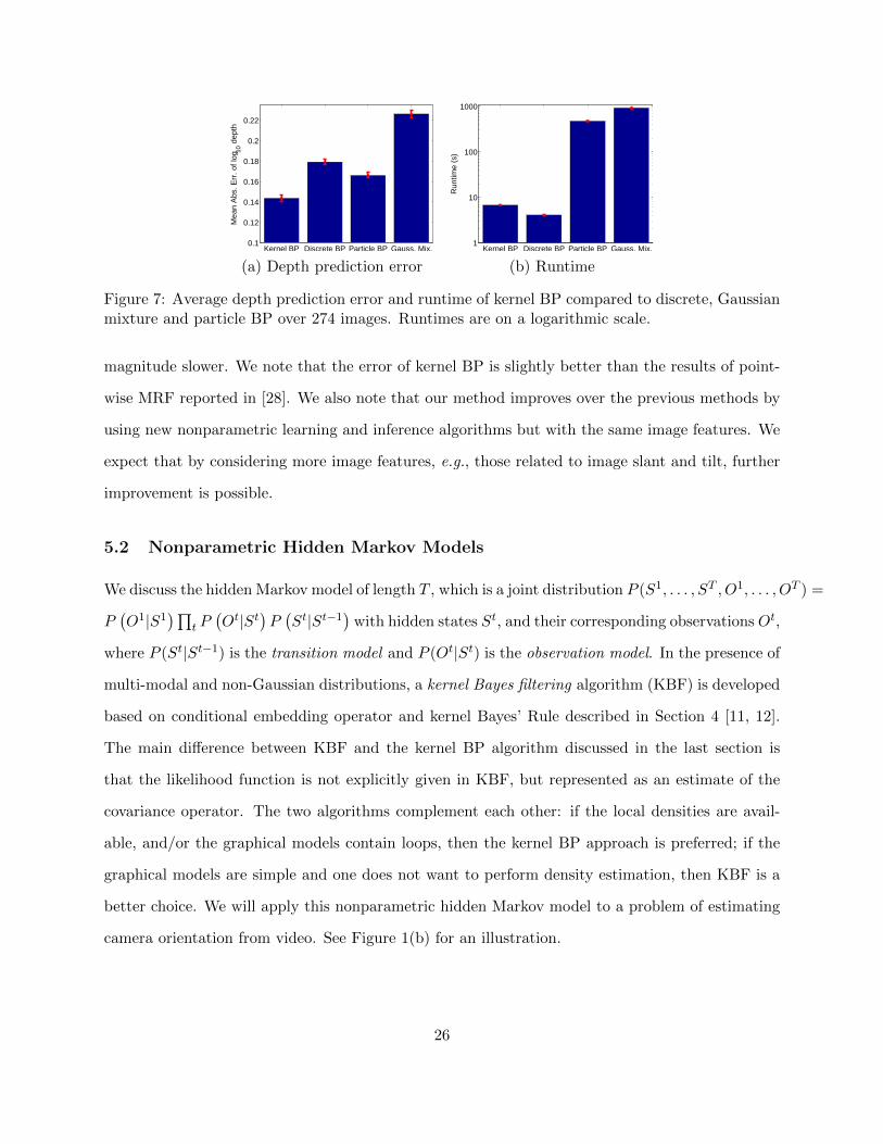
Our results were obtained by leave-one-out cross validation. For each test image, we ran discrete,

Gaussian mixture, particle, and kernel BP for 10 BP iterations. The average prediction error (MAE:

mean absolute error) and runtime are shown in Figures 7(a) and (b). Kernel BP produces the lowest

error (MAE=0.145) by a significant margin, while having a similar runtime to discrete BP. Gaussian

mixture and particle BP achieve better MAE than discrete BP, but their runtimes are two order of

25

Kernel BP Discrete BP Particle BP Gauss. Mix.0.1

0.12

0.14

0.16

0.18

0.2

0.22

Mea

n A

bs. E

rr. o

f log

10 d

epth

Kernel BP Discrete BP Particle BP Gauss. Mix.1

10

100

1000

Run

time

(s)

(a) Depth prediction error (b) Runtime

Figure 7: Average depth prediction error and runtime of kernel BP compared to discrete, Gaussianmixture and particle BP over 274 images. Runtimes are on a logarithmic scale.

magnitude slower. We note that the error of kernel BP is slightly better than the results of point-

wise MRF reported in [28]. We also note that our method improves over the previous methods by

using new nonparametric learning and inference algorithms but with the same image features. We

expect that by considering more image features, e.g., those related to image slant and tilt, further

improvement is possible.

5.2 Nonparametric Hidden Markov Models

We discuss the hidden Markov model of length T , which is a joint distribution P (S1, . . . , ST , O1, . . . , OT ) =

P(O1|S1

)∏t P(Ot|St

)P(St|St−1

)with hidden states St, and their corresponding observationsOt,

where P (St|St−1) is the transition model and P (Ot|St) is the observation model. In the presence of

multi-modal and non-Gaussian distributions, a kernel Bayes filtering algorithm (KBF) is developed

based on conditional embedding operator and kernel Bayes’ Rule described in Section 4 [11, 12].

The main difference between KBF and the kernel BP algorithm discussed in the last section is

that the likelihood function is not explicitly given in KBF, but represented as an estimate of the

covariance operator. The two algorithms complement each other: if the local densities are avail-

able, and/or the graphical models contain loops, then the kernel BP approach is preferred; if the

graphical models are simple and one does not want to perform density estimation, then KBF is a

better choice. We will apply this nonparametric hidden Markov model to a problem of estimating

camera orientation from video. See Figure 1(b) for an illustration.

26

5.2.1 Problem Formulation

In the framework of conditional embedding, we need to express P(St|St−1

)and P

(Ot|St

)with

samples. We thus assume that a training sample (s1, . . . , sT , o1, . . . , oT ) is available in the training

phase. In the testing phase, given a new sample (o1, . . . , oT ), we infer the hidden states (S1, . . . , ST ).

Note that in the training phase we assume that the sample on the hidden states is available. While

this is a restriction of the method, there are many situations where this assumption is satisfied; if

the measurement of hidden states is very expensive, we wish to estimate them from observations

based on a small number of training samples; when the hidden state can be observed with a time

delay, the real time estimation of the current hidden state may be necessary based on previous

data.

We focus on filtering, in which one queries the model for the posterior at some time step

conditioned on all past observations, though other operations such as smoothing and prediction are

also possible. Denote the history of the dynamical system as ht := (o1, . . . , ot). In filtering, one

recursively maintains a belief state, P (St+1|ht+1), in two steps: a prediction step and a conditioning

step. The first updates the distribution by multiplying by the transition model and marginalizing

out the previous time step: P (St+1|ht) = ESt|ht [P (St+1|St)]. The second conditions the distribution

on a new observation Ot+1 using Bayes’ rule: P (St+1|htot+1) ∝ P (ot+1|St+1)P (St+1|ht). The

derivation of the method is analogous to the sequential update rule for the standard linear Gaussian

models or hidden Markov model with discrete domains. The kernel Sum Rule and Bayes’ Rule in

Section 4 reduce the Bayesian computation into linear algebraic operations on Gram matrices.

5.2.2 Kernel Algorithm

The prediction and conditioning steps can be reformulated with respect to the kernel embeddings.

By maintaining the belief state recursively, we can assume that µSt|ht is known. Applying the

kernel Sum Rule to P (St+1|ht) = ESt|ht [P (St+1|St)], we have

µSt+1|ht = CSt+1|St µSt|ht , and C(St+1St+1)|ht = C(St+1St+1)|St µSt|ht . (31)

27

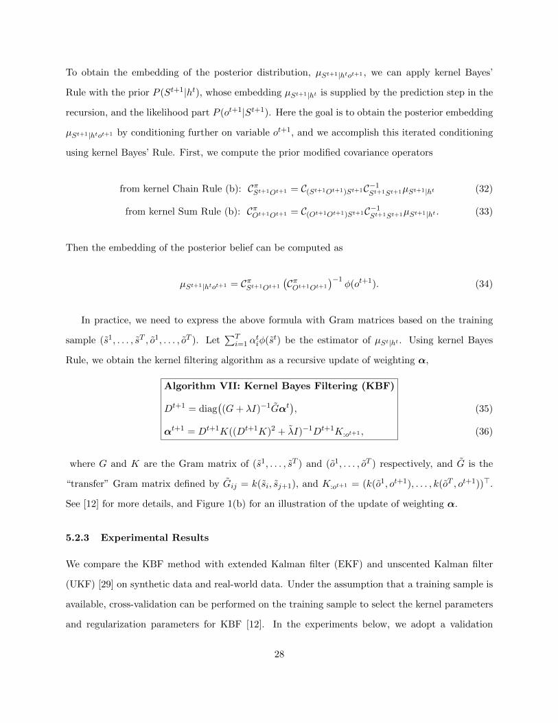
To obtain the embedding of the posterior distribution, µSt+1|htot+1 , we can apply kernel Bayes’

Rule with the prior P (St+1|ht), whose embedding µSt+1|ht is supplied by the prediction step in the

recursion, and the likelihood part P (ot+1|St+1). Here the goal is to obtain the posterior embedding

µSt+1|htot+1 by conditioning further on variable ot+1, and we accomplish this iterated conditioning

using kernel Bayes’ Rule. First, we compute the prior modified covariance operators

from kernel Chain Rule (b): CπSt+1Ot+1 = C(St+1Ot+1)St+1C−1St+1St+1µSt+1|ht (32)

from kernel Sum Rule (b): CπOt+1Ot+1 = C(Ot+1Ot+1)St+1C−1St+1St+1µSt+1|ht . (33)

Then the embedding of the posterior belief can be computed as

µSt+1|htot+1 = CπSt+1Ot+1

(CπOt+1Ot+1

)−1φ(ot+1). (34)

In practice, we need to express the above formula with Gram matrices based on the training

sample (s1, . . . , sT , o1, . . . , oT ). Let∑T

i=1 αtiφ(st) be the estimator of µSt|ht . Using kernel Bayes

Rule, we obtain the kernel filtering algorithm as a recursive update of weighting α,

Algorithm VII: Kernel Bayes Filtering (KBF)

Dt+1 = diag((G+ λI)−1Gαt

),

αt+1 = Dt+1K((Dt+1K)2 + λI)−1Dt+1K:ot+1 ,

(35)

(36)

where G and K are the Gram matrix of (s1, . . . , sT ) and (o1, . . . , oT ) respectively, and G is the

“transfer” Gram matrix defined by Gij = k(si, sj+1), and K:ot+1 = (k(o1, ot+1), . . . , k(oT , ot+1))>.

See [12] for more details, and Figure 1(b) for an illustration of the update of weighting α.

5.2.3 Experimental Results

We compare the KBF method with extended Kalman filter (EKF) and unscented Kalman filter

(UKF) [29] on synthetic data and real-world data. Under the assumption that a training sample is

available, cross-validation can be performed on the training sample to select the kernel parameters

and regularization parameters for KBF [12]. In the experiments below, we adopt a validation

28

approach by dividing the training sample in two.

We first applied the KBF algorithm to a simple nonlinear dynamical system, in which the degree

of nonlinearity can be controlled. The dynamics of the hidden state St = (ut, vt)> ∈ R2, are given by

(a) rotation in a circle: (ut+1, vt+1) = (cos θt+1, sin θt+1), θt+1 = θt+ 0.3 with θt = arctan(|vt|/|ut|),

and (b) oscillatory rotation: (ut+1, vt+1) = (1 + 0.4 sin(8θt+1))(cos θt+1, sin θt+1), θt+1 = θt + 0.4.

The observation ot+1 includes noise: ot+1 = (ut+1, vt+1)>+ ξ with ξ ∼ N(0, 0.08I2) in both (a) and

(b). Note that the dynamics of (ut, vt) are nonlinear even in (a).

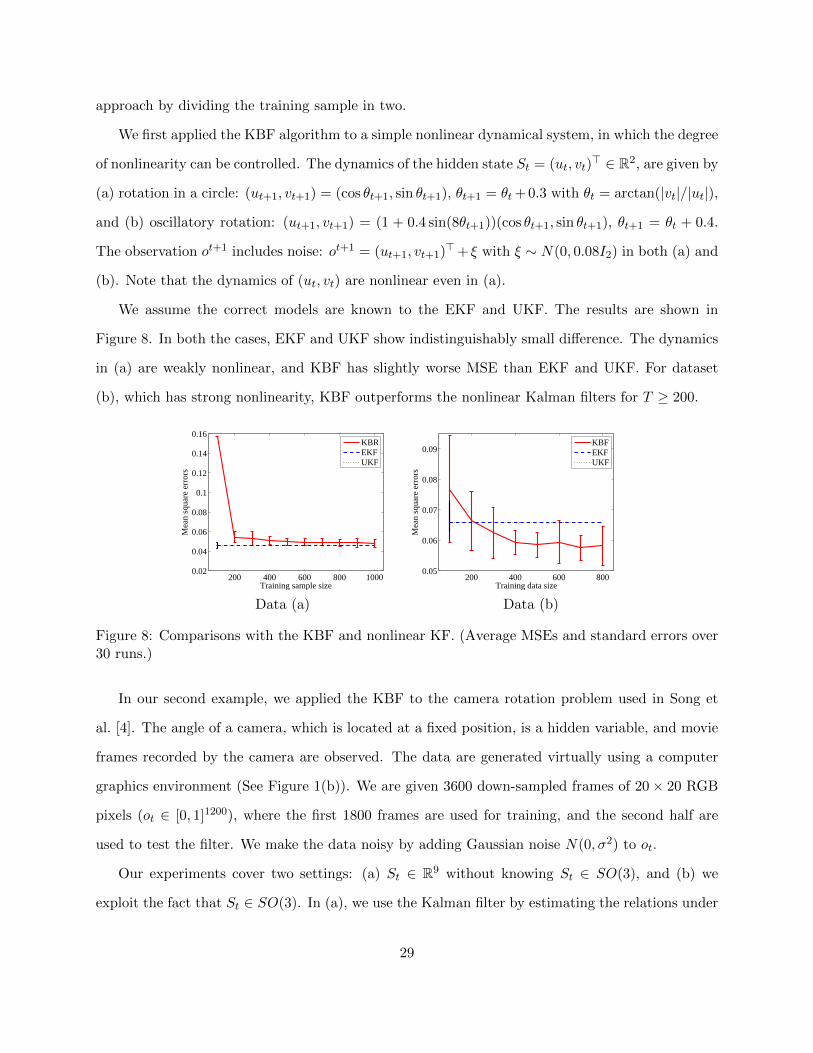
We assume the correct models are known to the EKF and UKF. The results are shown in

Figure 8. In both the cases, EKF and UKF show indistinguishably small difference. The dynamics

in (a) are weakly nonlinear, and KBF has slightly worse MSE than EKF and UKF. For dataset

(b), which has strong nonlinearity, KBF outperforms the nonlinear Kalman filters for T ≥ 200.

200 400 600 800 10000.02

0.04

0.06

0.08

0.1

0.12

0.14

0.16

Training sample size

Mea

n sq

uare

err

ors

KBREKFUKF

200 400 600 8000.05

0.06

0.07

0.08

0.09

Training data size

Mea

n sq

uare

err

ors

KBFEKFUKF

Data (a) Data (b)

Figure 8: Comparisons with the KBF and nonlinear KF. (Average MSEs and standard errors over30 runs.)

In our second example, we applied the KBF to the camera rotation problem used in Song et

al. [4]. The angle of a camera, which is located at a fixed position, is a hidden variable, and movie

frames recorded by the camera are observed. The data are generated virtually using a computer

graphics environment (See Figure 1(b)). We are given 3600 down-sampled frames of 20× 20 RGB

pixels (ot ∈ [0, 1]1200), where the first 1800 frames are used for training, and the second half are

used to test the filter. We make the data noisy by adding Gaussian noise N(0, σ2) to ot.

Our experiments cover two settings: (a) St ∈ R9 without knowing St ∈ SO(3), and (b) we

exploit the fact that St ∈ SO(3). In (a), we use the Kalman filter by estimating the relations under

29

a linear assumption, and the KBF with Gaussian kernels for St and Ot as Euclidean vectors. In (b),

for the Kalman Filter, St is represented by a quaternion, which is a standard vector representation

of rotations; for the KBF the kernel k(A,B) = Tr[ABT ] is used for St, and St is estimated within

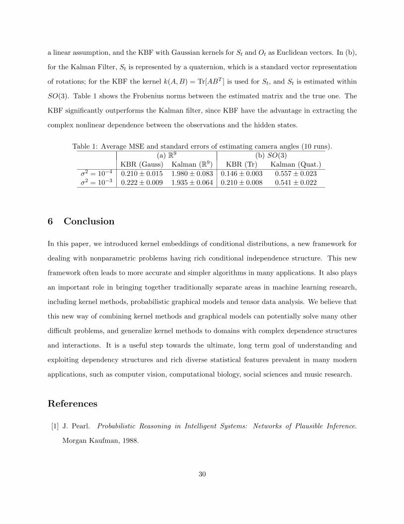
SO(3). Table 1 shows the Frobenius norms between the estimated matrix and the true one. The

KBF significantly outperforms the Kalman filter, since KBF have the advantage in extracting the

complex nonlinear dependence between the observations and the hidden states.

Table 1: Average MSE and standard errors of estimating camera angles (10 runs).(a) R9 (b) SO(3)

KBR (Gauss) Kalman (R9) KBR (Tr) Kalman (Quat.)

σ2 = 10−4 0.210± 0.015 1.980± 0.083 0.146± 0.003 0.557± 0.023σ2 = 10−3 0.222± 0.009 1.935± 0.064 0.210± 0.008 0.541± 0.022

6 Conclusion

In this paper, we introduced kernel embeddings of conditional distributions, a new framework for

dealing with nonparametric problems having rich conditional independence structure. This new

framework often leads to more accurate and simpler algorithms in many applications. It also plays

an important role in bringing together traditionally separate areas in machine learning research,

including kernel methods, probabilistic graphical models and tensor data analysis. We believe that

this new way of combining kernel methods and graphical models can potentially solve many other

difficult problems, and generalize kernel methods to domains with complex dependence structures

and interactions. It is a useful step towards the ultimate, long term goal of understanding and

exploiting dependency structures and rich diverse statistical features prevalent in many modern

applications, such as computer vision, computational biology, social sciences and music research.

References

[1] J. Pearl. Probabilistic Reasoning in Intelligent Systems: Networks of Plausible Inference.

Morgan Kaufman, 1988.

30

[2] E. Sudderth, A. Ihler, W. Freeman, and A. Willsky. Nonparametric belief propagation. In

Proc. IEEE Conf. Computer Vision and Pattern Recognition, 2003.

[3] B. W. Silverman. Density Estimation for Statistical and Data Analysis. Monographs on

statistics and applied probability. Chapman and Hall, London, 1986.

[4] L. Song, J. Huang, A. J. Smola, and K. Fukumizu. Hilbert space embeddings of conditional

distributions. In Proceedings of the International Conference on Machine Learning, 2009.

[5] L. Song, A. Gretton, and C. Guestrin. Nonparametric tree graphical models. In Proc. Intl.

Conference on Artificial Intelligence and Statistics, 2010.

[6] L. Song, B. Boots, S. Siddiqi, G. Gordon, and A. J. Smola. Hilbert space embeddings of hidden

markov models. In International Conference on Machine Learning, 2010.

[7] L. Song, A. Gretton, D. Bickson, Y. Low, and C. Guestrin. Kernel belief propagation. In Proc.

Intl. Conference on Artificial Intelligence and Statistics, 2011.

[8] L. Song, A. Parikh, and E.P. Xing. Kernel embeddings of latent tree graphical models. In

Advances in Neural Information Processing Systems, volume 25, 2011.

[9] S. Grunewalder, G. Lever, L. Baldassarre, M. Pontil, and A. Gretton. Modeling transition

dynamics in MDPs with RKHS embeddings. In Proceedings of the International Conference

on Machine Learning, 2012.

[10] Y. Nishiyama, A. Boularias, A. Gretton, and K. Fukumizu. Hilbert space embeddings of

POMDPs. In Conference on Uncertainty in Artificial Intelligence, 2012.

[11] K. Fukumizu, L. Song, and A. Gretton. Kernel Bayes’ rule. In Neural Information Processing

Systems, 2011.

[12] K. Fukumizu, L. Song, and A. Gretton. Kernel Bayes’ rule: Bayesian inference with positive

definite kernels. In accepted to JMLR, 2012.

[13] B. Scholkopf, K. Tsuda, and J.-P. Vert. Kernel Methods in Computational Biology. MIT Press,

Cambridge, MA, 2004.

31

[14] K. Fukumizu, F. R. Bach, and M. I. Jordan. Dimensionality reduction for supervised learning

with reproducing kernel Hilbert spaces. Journal of Machine Learning Research, 5:73–99, 2004.

[15] A. Berlinet and C. Thomas-Agnan. Reproducing Kernel Hilbert Spaces in Probability and

Statistics. Kluwer, 2004.

[16] A. J. Smola, A. Gretton, L. Song, and B. Scholkopf. A Hilbert space embedding for distribu-

tions. In Proceedings of the International Conference on Algorithmic Learning Theory, volume

4754, pages 13–31. Springer, 2007.

[17] B. Sriperumbudur, A. Gretton, K. Fukumizu, G. Lanckriet, and B. Scholkopf. Injective Hilbert

space embeddings of probability measures. In Proc. Annual Conf. Computational Learning

Theory, pages 111–122, 2008.

[18] B. Sriperumbudur, A. Gretton, K. Fukumizu, G. Lanckriet, and B. Scholkopf. Hilbert space

embeddings and metrics on probability measures. Journal of Machine Learning Research,

11:1517–1561, 2010.

[19] A. Gretton, K. Borgwardt, M. Rasch, B. Schoelkopf, and A. Smola. A kernel two-sample test.

Journal of Machine Learning Research, 13:723–773, 2012.

[20] A. Gretton, K. Fukumizu, C.-H. Teo, L. Song, B. Scholkopf, and A. J. Smola. A kernel

statistical test of independence. In Advances in Neural Information Processing Systems 20,

pages 585–592, Cambridge, MA, 2008. MIT Press.

[21] A. Gretton, B. Sriperumbudur, D. Sejdinovic, S. Balakrishnan, M. Pontil, K. Fukumizu, et al.

Optimal kernel choice for large-scale two-sample tests. In Advances in Neural Information

Processing Systems 25, pages 1214–1222, 2012.

[22] S. K. Zhou and R. Chellappa. From sample similarity to ensemble similarity: Probabilistic

distance measures in reproducing kernel Hilbert space. IEEE Transactions on Pattern Analysis

and Machine Intelligence, 28(6):917–929, 2006.

32

[23] S. Fine and K. Scheinberg. Efficient SVM training using low-rank kernel representations.

Journal of Machine Learning Research, 2:243–264, 2001.

[24] S. Grunewalder, G. Lever, L. Baldassarre, S. Patterson, A. Gretton, and M. Pontil. Conditional

mean embeddings as regressors. In Proceedings of the International Conference on Machine

Learning, 2012.

[25] S. Mika, B. Scholkopf, A. J. Smola, K.-R. Muller, Matthias Scholz, and G. Ratsch. Kernel

PCA and de-noising in feature spaces. In M. S. Kearns, S. A. Solla, and D. A. Cohn, editors,

Advances in Neural Information Processing Systems 11, pages 536–542. MIT Press, 1999.

[26] A. Ihler and D. McAllester. Particle belief propagation. In Proc. Intl. Conference on Artificial

Intelligence and Statistics, pages 256–263, 2009.

[27] C. Andrieu, N. de Freitas, A. Doucet, and M. I. Jordan. An introduction to mcmc for machine

learning. Machine Learning, 50:5–43, 2003.

[28] A. Saxena, M. Sun, and A.Y. Ng. Make3d: Learning 3d scene structure from a single still

image. IEEE Trans. Pattern Anal. Mach. Intell., 31(5):824–840, 2009.

[29] S.J. Julier and J.K. Uhlmann. New extension of the kalman filter to nonlinear systems. In

AeroSense’97, pages 182–193. International Society for Optics and Photonics, 1997.

33