Kernel Density Estimation for Target Trajectory Prediction

Vahab Akbarzadeh1, Christian Gagne2, and Marc Parizeau3

Abstract— This paper proposes the use of a kernel densityestimation to measure similarities between trajectories. Thesimilarities are then used to predict the future locations of atarget. For a given environment with a history of previous targettrajectories, the goal is to establish a probabilistic frameworkto predict the future trajectory of currently observed targetsbased on their recent moves. Instead of clustering trajectoriesinto groups, we calculate the similarity between a given testtrajectory and the set of all past trajectories in a dataset. Next,we use a weighted mechanism for prediction, that can be usedin target tracking and collision avoidance applications. Theproposed method is compared with two other commonly usedsimilarity models (PCA and LCSS) over a dataset of simulatedtrajectories, and two datasets of real observations. Results showthat the proposed method significantly outperforms the existingmodels for those datasets and experimental settings.

I. INTRODUCTION

Trajectory prediction is the process of estimating the futurelocation of a target moving inside an environment. A trajec-tory is usually modelled as a sequence of observed locationsfor the target. Therefore, in trajectory prediction, the goal isto predict the future location of a given target, given a historyof previous target locations. Trajectory prediction has manyapplications in robotics. For example, in an environmentwhere humans and robots coexist, the trajectory of the robotscan be determined based on human trajectories, as the systemtries to avoid possible collisions between robots and humans.Therefore, it is crucial to have an accurate estimate for thefuture positions of the humans [6].

A simple approach for this problem is to perform anestimation using only an on-going trajectory of the sametarget. Kalman Filters [4] and Particle Filters [3] are twoclassical methods commonly used for this purpose. Theproblem with these approaches is that they are not able topredict far into the future. For example, if one uses particlefiltering (or Kalman filtering) to predict 10 time steps ahead,the prediction variance will grow 10 times larger than the onetime step variance, which would make the method hardlyusable for most applications, as the prediction uncertaintycould rapidly become larger than the area under study.

A more informed approach is to exploit the history of othertargets that have already traversed the same environment, topredict the trajectory of future targets. To exploit the historyof previous targets, some approaches require the calculationof the similarity between two trajectories. Here, the two

Authors are with Laboratoire de vision et systemes numeriques,Departement de genie electrique et de genie informatique, Universite Laval,Quebec (Quebec), Canada. E-mails:1Vahab.Akbarzadeh.1@ulaval.ca2Christian.Gagne@gel.ulaval.ca3Marc.Parizeau@gel.ulaval.ca

trajectories are that of a new target and another trajectoryfrom the set of trajectories of previous targets. There areseveral approaches proposed to solve this problem. Forinstance, Bashir et al. [1] proposed to determine the dissim-ilarity between two trajectories using the Euclidean distancebetween the Principal Component Analysis (PCA) coeffi-cients of each trajectory. Dynamic Time Warping (DTW)[5], and Longest Common Subsequence (LCSS) [9] are twoother methods that calculate similarity through subsequencealignment. They have been shown to produce stable results[11].

The mentioned similarity-based prediction methods can beviewed as non-parametric approaches for the problem. Theparametric approaches (e.g. hidden Markov models (HMM)[7], or inverse reinforcement learning [13]) have also beenapplied for the prediction problem.

Compared to parametric methods, non-parametric methodshave desirable properties for trajectory prediction, such astheir ability to work in an online fashion. In other words,with parametric methods, the addition of new trajectories inthe history dataset implies the re-estimation of all systemparameters, while this is not the case for non-parametricmethods. This is an important property for the trajectoryprediction problem, because new trajectories are detected allthe time and they should be added to the history dataset. Non-parametric methods have the advantage of being insensitiveto the addition of new trajectories, as each prediction iscomputed on-demand over the history dataset, with littleor no other computation required beforehand. However, thecomputation required is proportional to the history datasetsize, such that for a large set of trajectories observed,one should limit computation by restricting the size of thehistory dataset used in some way (e.g., through a slidingwindow). Specifically, in the case where the obstacles in theenvironment are mobile, the combination of online trajectoryaddition and the sliding variable becomes important, as themost recent trajectories should be used for prediction of newtrajectories.

Besides, the parameters of a parametric method can be finetuned for a specific problem, but usually differ from problemto problem. For example, in the HMM approaches, the choiceof the number and form of hidden states (which could be linesegments [7], mixture of Gaussians [2], or Voronoi diagrams[8], etc.) is different for different environments.

In this paper, we propose to use kernel density estimation(KDE) as a non-parametric method, to model the similaritybetween two trajectories, and to use that similarity to predictthe future locations of targets. Moreover, instead of clusteringtrajectories into groups, we calculate the similarity between

a given test trajectory and the set of all trajectories inthe history dataset. Next, we use a weighted mechanismfor prediction. The performance of the proposed similaritymeasure is compared with the well-known LCSS and PCAmethods over a dataset of simulated trajectories and twodatasets of real observations.

II. PROBLEM DEFINITION

Trajectory prediction is the process of estimating the futurelocation of a given target using the information of its previousmovements and the movements that other targets have madein the same environment. More precisely, let T(t)

j representan on-going target’s trajectory in an environment Ξ, currentlybeing observed at time t, since its arrival at time tj . We wishto predict the location of the target after s time steps (i.e.,T

(t+s)

j ) as accurately as possible.We build a probabilistic model to represent the target’s

future location. Let X(t+s)j denote over the sample space of

all locations q ∈ Ξ, a discrete random variable for target Tjat time t + s. Variable X

(t+s)j is defined by a probability

mass function P (X(t+s)j = q) which returns the probability

of target Tj being at location q at time t + s. For brevity,we note this value as P(t+s)

jq .The goal is to incrementally learn the probabilistic model

for each target as it moves within the environment, using theinformation of N previously observed target trajectories Ti

in the same environment, T = {T1,T2, . . . ,TN}.The performance of the trajectory prediction method is

measured using the expected value of distance betweenthe prediction and the actual location of the target. Moreprecisely, using the law of the unconscious statistician, theprediction error E(t+s)

j for location p(t+s)j of a test trajectory

Tj , at time t+ s, is defined as:

E(t+s)j =

∑q∈Ξ

P(t+s)jq

∥∥∥q− p(t+s)j

∥∥∥2, (1)

where the sum of the Euclidean distances (|| · ||2) betweenthe actual location of the target and all possible positions qin the environment is weighted by the predicted probabilityP(t+s)jq that the target will be at position q. The goal of the

prediction method is to identify the prediction mechanismwhich gives the minimum value for the prediction error:

P∗(t+s)jq = argminP(t+s)

jq

E(t+s)j . (2)

III. THE PROPOSED METHOD

We propose to carry out the prediction using the similaritymeasure between the trajectories. The principal assumptionis that the similarity between the previous locations anddisplacements of two trajectories is directly related to thecloseness of their future locations. The main problem is howto define the similarity between two trajectories.

More formally, at a time step t, we wish to measurethe similarity S(T

(t)j ,Tm) between the current state T

(t)j

of an ongoing trajectory and the whole history of anothertrajectory Tm ∈ T. Then, we form a four dimensional

space, where the state of a trajectory at one time stepis represented by a point in this space, consisting of itscurrent location p

(t)j = (x

(t)j , y

(t)j ) and its most recent

displacement ∆p(t)j = (∆x

(t)j ,∆y

(t)j ). As a result we have

T(t)j = {x(t)

j , y(t)j ,∆x

(t)j ,∆y

(t)j }.

In the mentioned four dimensional space we estimatethe density of trajectory Tm, and we define the similaritybetween the state of trajectory Tj at time t, as its valuewithin the density estimated for the trajectory Tm. Moreformally we have:

S(T(t)j ,Tm) = FTm(T

(t)j ), (3)

where S(., .) is the similarity function and FTm(T

(t)j ) is

the density estimated for trajectory Tm evaluated at pointT

(t)j . For density estimation, we use the non-parametric

multivariate kernel method. More precisely we have:

FTm(z) =

1

nm

nm∑t=1

K(T(t)m , z,hm), (4)

where nm is the total number of displacements of target Tm

and hm = {h1, h2, h3, h4} are the bandwidth parameters fortrajectory Tm along the four mentioned dimensions. Theseparameters define the length-scale of the function for locationand displacement, respectively. Informally speaking, h1, andh2 define how far two locations should be in the environmentto be considered far (along the x and y dimensions), andh3, and h4 define how much the directions of the twodisplacements should diverge before they are considereddifferent (along the ∆x and ∆y dimensions).

For the kernel function K(., ., .), we use the normaldistribution defined as:

K(z, z′,h) =

4∏d=1

1

hdK

(zd − z′dhd

), (5)

K(u) =1√2π

exp

(−u

2

2

). (6)

A. The problem of missing observations

The mentioned similarity function is defined in four di-mensions and therefore difficult to visualize. As a resultwe present the behaviour of the similarity function in aone dimensional space (Fig. 1). In this figure, there aretwo consecutive observations at positions 1 and 5, and weobserve that the similarity is higher close to those points. Inthe figure, the dotted lines represent the underlying normaldistributions we mapped over each observation.

The assumption behind the similarity function is that thetrajectory of the history target Tm has been observed at alltime steps. As we will see in Sec. IV, this is not the case inmost real datasets. In reality the time step difference betweenconsecutive observations of the same trajectory might bedifferent. For example, assume that for the data presentedin Fig. 1, the time difference between the two observationsis four time steps (instead of one). The current model isnot compatible with this assumption and therefore shouldbe modified. One possibility is to evenly divide the space

4 3 2 1 0 1 2 3 4 5 6 7 8 9 100.00

0.05

0.10

0.15

0.20

0.25Sim

ilari

ty

Fig. 1: The behaviour of the similarity function in onedimension.

4 3 2 1 0 1 2 3 4 5 6 7 8 9 100.00

0.05

0.10

0.15

0.20

0.25

Sim

ilari

ty

Fig. 2: The behaviour of the similarity function with un-known intermediate observations and fixed bandwidth pa-rameters.

between the two observations and add each interpolatedpoint as an observation. In this model all the newly createdobservations would have equal bandwidth parameters h. Thismodel is presented in Fig. 2.

The problem with this approach is that it assumes thatthe intermediate observations, which we did not actuallyobserve, have the same bandwidth parameter as the actualobservations we made. For the example given in Fig. 2, thesimilarity at point 3 is higher than that of point 5, while wehad an observation at point 5, but none at point 3.

For that reason, we propose a model in which the band-width parameter of the interpolated observations increaselinearly as the interpolated point is located further awayfrom an actual observation. Fig. 3 represents our model forthe example given before. As can be seen, the bandwidthparameter is the same for the points where we had anobservation (points 1 and 5), and the bandwidth parameterincreases as we move away from the observations. In thesame way, we modify the similarity equation (Eq. 4), so thatthe bandwidth parameter is a function of the observation,and therefore not fixed for all points. The modified versionof the similarity equation (Eq. 4) is as follows:

FTm(z) =

1

nm

nm∑t=1

K(T(t)m , z,h(t)

m ), (7)

4 3 2 1 0 1 2 3 4 5 6 7 8 9 100.00

0.05

0.10

0.15

0.20

0.25

Sim

ilari

ty

Fig. 3: The behaviour of the similarity function with un-known intermediate observations and variable bandwidthparameters.

where, in the new formula, the bandwidth parameter h(t)m is

defined for each trajectory m at each time step t.

B. Parameter estimation

The only parameters of the KDE method that shouldbe decided are the bandwidth parameters. As previouslymentioned, the bandwidth parameters define the distance atwhich two points are considered close. Therefore, a meansof determining the value of the bandwidth parameters for theinterpolated points is needed.

We are proposing to calculate the bandwidth parametersby first interpolating the intermediate points. Following this,the bandwidth parameters are computed by maximizing aleave-one-out cross-validation likelihood:

FTm−i(Tm) =1

nm − 1

nm∑t=1,t6=i

K(T(t)m ,T(i)

m ,hm). (8)

In other words, in order to evaluate a parameter hm fortrajectory Tm, only one of the displacements of the trajectory(T(i)

m ) is removed from the summation and the likelihoodof the similarity function is evaluated at that point. For agiven bandwidth parameter, the process is repeated for alldisplacements in the trajectory. Therefore the final processis:

nm∏i=1

FTm−i(Tm) =

1(nm−1)nm

nm∏i=1

nm∑t=1,t6=i

K(T(t)m ,T

(i)m ,hm).

(9)

In the given formula the multiplicands are usually smalland the final product leads to underflow. Therefore it is moreconvenient to maximize the log of the likelihood:

nm∑i=1

log[FTm−i(Tm)

]= −nm log (nm − 1)+

nm∑i=1

log

[nm∑

t=1,t6=iK(T

(t)m ,T

(i)m ,hm)

].

(10)

Taking the derivatives of the given formula with respectto the bandwidth parameters leads to complex equations,which cannot be solved in a closed form. Therefore, we are

proposing to adjust the parameters of the method by a linesearch conducted within the range [1, 20] in increments of0.5, independently for each bandwidth parameter. Indeed,according to our formulation of the Gaussian kernel (seeEq. 5), the effect of each bandwidth parameter on thelikelihood is not related to the others. The best value for eachbandwidth parameter is chosen as the value of the parameterfor each trajectory.

Notice that the mentioned formula defines the bandwidthparameter for the observed points. For each interpolatedpoint, we define a level property L(T

(t)j ), which measures

the distance between the mentioned point and the closestobserved point. For the example given in Fig. 2, points 2and 4 have level 2, and point 3 has level 3. The observedpoints (1 and 5) both have level 1. Using this formula thebandwidth parameter is defined as:

h(t)j = L(T

(t)j )× hj , (11)

where hj is the base bandwidth parameter calculated usingthe method proposed in Eq. 10.

C. Prediction using the similarity function

Once the similarities have been calculated, at each timestep, the similarity function behaves as a weighting parameterthat can be used to predict the future locations of target T(t)

j

as a weighted sum of the trajectory of the previous targets.More precisely we have:

w(t)ji =

S(T(t)j ,Ti)∑

Tm∈TS(T

(t)j ,Tm)

, (12)

where w(t)ji is the normalized similarity between the displace-

ment of target Tj at time t and the whole trajectory Ti ∈ T.Using this formulation, the future location of a target is adiscrete probability distribution over environment Ξ, wherethe probability of the target associated with Tj being at eachlocation q ∈ Ξ after s time steps from current time t isdefined as:

P(t+s)jq =

∑Tm∈T

w(t)jm1(T(θ∗+s)

m ,q), (13)

where function 1(T(θ∗+s)m ,q) returns one if the target that

generated Tm was at location q at time θ∗ + s, and zerootherwise.

In order to predict the next locations of trajectory T(t)j

at each time step among all of the displacements T(θ)m of

a sample trajectory Tm, the displacement which is mostsimilar with the current displacement T

(t)j of target Tj

should be found. This most similar displacement occurs attime step:

θ∗ = argmaxθ

S(T(θ)m ,T

(t)j ). (14)

The whole process of trajectory prediction and perfor-mance evaluation is shown for a simple example in Fig. 4. Asbefore, Tj is the test trajectory for which we want to predictfuture locations, and we have the history of two reference

Fig. 4: Target trajectory prediction process.

trajectories T1 and T2. We will use the reference trajectoriesfor predicting the location of the test trajectory. Target Tj

is currently at the third time step, t = 3, and we want todetermine its location after four time steps, s = 4.

First, the similarity between the last displacement ofthe test trajectory (T(3)

j ) and the reference trajectories iscalculated. Let us assume that S(T

(3)j ,T1) = 0.2, and

that S(T(3)j ,T2) = 0.3. Therefore (using Eq. 12) we have

w(3)j1 = 0.4, and w

(3)j2 = 0.6. Next, we use Eq. 14 to

determine the displacements in the reference trajectories thatmaximize similarity with the current displacement of the testtrajectory (T(θ∗)

1 , T(θ∗)2 ). A non-zero prediction probability

is assigned to the two reference trajectories, which are usedto predict the future locations of the test trajectory (T(7)

j ).To evaluate the performance, the distance between our

prediction and the actual location of the test trajectory iscalculated (‖q1−p

(7)j ‖2,‖q2−p

(7)j ‖2). Based on this result

the performance of our prediction would be E(7)j = 0.4 ×

‖q1 − p(7)j ‖2 + 0.6× ‖q2 − p

(7)j ‖2.

IV. EXPERIMENTS

In the following, we are presenting an experimentalcomparison of the proposed KDE-based similarity measurewith two other well-known similarity measures, LCSS andPCA. Three different experimental settings are tested, onewith simulated trajectories that we have designed and twoconfigurations based on datasets of real targets tracked in2D.

The trajectory prediction is computed in an online fash-ion. Thus, the history of reference trajectories T begin bycontaining the first trajectory T = {T1}. Then, every time anew trajectory Tj appears in the environment, its trajectoryis predicted using the reference trajectories in T, and onceits trajectory is completed, it is added to the referencetrajectories T = T ∪Tj .

As mentioned previously in Sec. III-A, in most realdatasets the time difference between consecutive displace-ments of trajectories is not constant. This is why the variablebandwidth parameter was defined for the kernel densityestimation method. This is also the case for the two realdatasets we present here. In our experiments, we usedonly the trajectories for which the time difference betweenconsecutive displacements is less than 10 time steps. If the

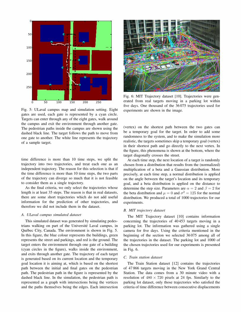
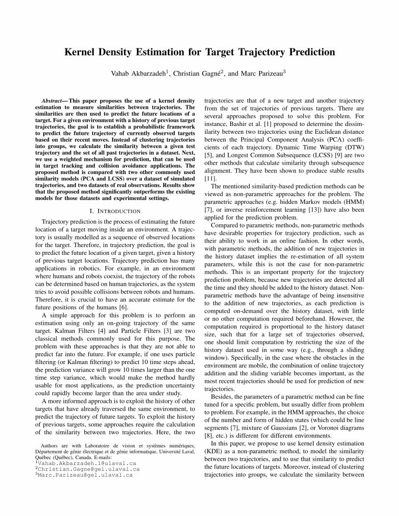
Fig. 5: ULaval campus map and simulation setting. Eightgates are used, each gate is represented by a cyan circle.Targets can enter through any of the eight gates, walk aroundthe campus and exit the environment through another gate.The pedestrian paths inside the campus are shown using thedashed black line. The target follows the path to move fromone gate to another. The white line represents the trajectoryof a sample target.

time difference is more than 10 time steps, we split thetrajectory into two trajectories, and treat each one as anindependent trajectory. The reason for this selection is that ifthe time difference is more than 10 time steps, the two partsof the trajectory can diverge so much that it is not feasibleto consider them as a single trajectory.

As the final criteria, we only select the trajectories whoselength is at least 35 steps. The reason is that in real datasets,there are some short trajectories which do not add usefulinformation for the prediction of other trajectories, andtherefore we did not include them in the dataset.

A. ULaval campus simulated dataset

This simulated dataset was generated by simulating pedes-trians walking on part of the Universite Laval campus, inQuebec City, Canada. The environment is shown in Fig. 5.In this figure, the blue colour represents the buildings, greenrepresents the street and parkings, and red is the ground. Thetarget enters the environment through one gate of a building(cyan circles in the figure), walks inside the environment,and exits through another gate. The trajectory of each targetis generated based on its current location and the temporarygoal location it is aiming at, which is based on the shortestpath between the initial and final gates on the pedestrianpath. The pedestrian path in the figure is represented by thedashed black line. In the simulation, the pedestrian path isrepresented as a graph with intersections being the verticesand the paths themselves being the edges. Each intersection

Fig. 6: MIT Trajectory dataset [10]. Trajectories were gen-erated from real targets moving in a parking lot withinfive days. One thousand of the 36 075 trajectories used forexperiments are shown in the image.

(vertex) on the shortest path between the two gates canbe a temporary goal for the target. In order to add somerandomness to the system, and to make the simulation morerealistic, the targets sometimes skip a temporary goal (vertex)in their shortest path and go directly to the next vertex. Inthe figure, this phenomena is shown at the bottom, where thetarget diagonally crosses the street.

At each time step, the next location of a target is randomlychosen from a distribution that results from the (normalized)multiplication of a beta and a Gaussian distribution. Moreprecisely, at each time step, a normal distribution is appliedon the angle between the target’s location and its temporarygoal, and a beta distribution is applied on the distance todetermine the step size. Parameters are α = 2 and β = 2 forthe beta distribution and µ = 0 and σ2 = 125 for the normaldistribution. We produced a total of 1000 trajectories for ourexperiments.

B. MIT trajectory dataset

The MIT Trajectory dataset [10] contains informationconcerning the trajectories of 40 453 targets moving in aparking lot. The information was gathered using a singlecamera for five days. Using the criteria mentioned in thebeginning of the section we selected 36 075 among all ofthe trajectories in the dataset. The parking lot and 1000 ofthe chosen trajectories used for our experiments is presentedin Fig. 6.

C. Train station dataset

The Train Station dataset [12] contains the trajectoriesof 47 866 targets moving in the New York Grand CentralStation. The data comes from a 30 minute video with aresolution of 480 × 720 pixels at 24 fps. Similarly to theparking lot dataset, only those trajectories who satisfied thecriteria of time difference between consecutive displacements

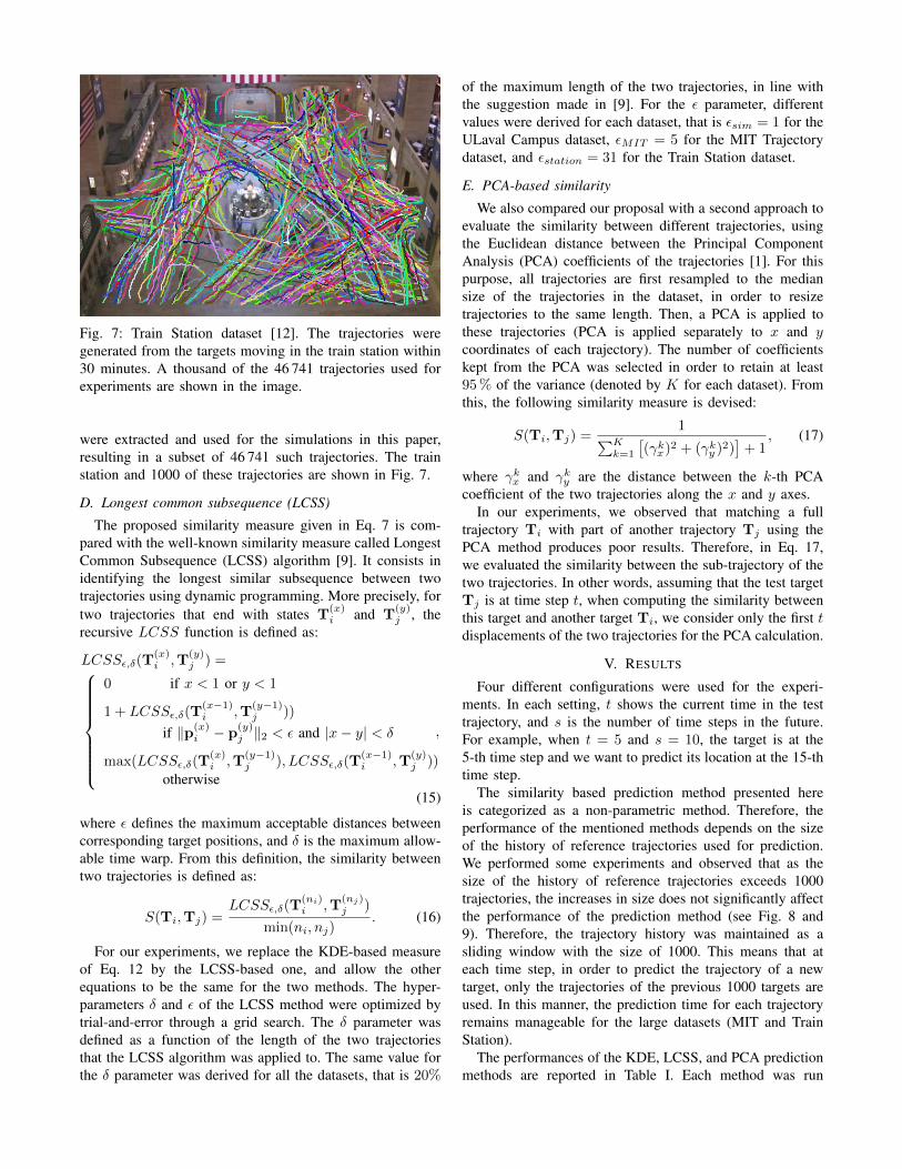
Fig. 7: Train Station dataset [12]. The trajectories weregenerated from the targets moving in the train station within30 minutes. A thousand of the 46 741 trajectories used forexperiments are shown in the image.

were extracted and used for the simulations in this paper,resulting in a subset of 46 741 such trajectories. The trainstation and 1000 of these trajectories are shown in Fig. 7.

D. Longest common subsequence (LCSS)

The proposed similarity measure given in Eq. 7 is com-pared with the well-known similarity measure called LongestCommon Subsequence (LCSS) algorithm [9]. It consists inidentifying the longest similar subsequence between twotrajectories using dynamic programming. More precisely, fortwo trajectories that end with states T

(x)i and T

(y)j , the

recursive LCSS function is defined as:

LCSSε,δ(T(x)i ,T

(y)j ) =

0 if x < 1 or y < 1

1 + LCSSε,δ(T(x−1)i ,T

(y−1)j ))

if ‖p(x)i − p

(y)j ‖2 < ε and |x− y| < δ

max(LCSSε,δ(T(x)i ,T

(y−1)j ), LCSSε,δ(T

(x−1)i ,T

(y)j ))

otherwise

,

(15)

where ε defines the maximum acceptable distances betweencorresponding target positions, and δ is the maximum allow-able time warp. From this definition, the similarity betweentwo trajectories is defined as:

S(Ti,Tj) =LCSSε,δ(T

(ni)i ,T

(nj)j )

min(ni, nj). (16)

For our experiments, we replace the KDE-based measureof Eq. 12 by the LCSS-based one, and allow the otherequations to be the same for the two methods. The hyper-parameters δ and ε of the LCSS method were optimized bytrial-and-error through a grid search. The δ parameter wasdefined as a function of the length of the two trajectoriesthat the LCSS algorithm was applied to. The same value forthe δ parameter was derived for all the datasets, that is 20%

of the maximum length of the two trajectories, in line withthe suggestion made in [9]. For the ε parameter, differentvalues were derived for each dataset, that is εsim = 1 for theULaval Campus dataset, εMIT = 5 for the MIT Trajectorydataset, and εstation = 31 for the Train Station dataset.

E. PCA-based similarity

We also compared our proposal with a second approach toevaluate the similarity between different trajectories, usingthe Euclidean distance between the Principal ComponentAnalysis (PCA) coefficients of the trajectories [1]. For thispurpose, all trajectories are first resampled to the mediansize of the trajectories in the dataset, in order to resizetrajectories to the same length. Then, a PCA is applied tothese trajectories (PCA is applied separately to x and ycoordinates of each trajectory). The number of coefficientskept from the PCA was selected in order to retain at least95 % of the variance (denoted by K for each dataset). Fromthis, the following similarity measure is devised:

S(Ti,Tj) =1∑K

k=1

[(γkx)2 + (γky )2)

]+ 1

, (17)

where γkx and γky are the distance between the k-th PCAcoefficient of the two trajectories along the x and y axes.

In our experiments, we observed that matching a fulltrajectory Ti with part of another trajectory Tj using thePCA method produces poor results. Therefore, in Eq. 17,we evaluated the similarity between the sub-trajectory of thetwo trajectories. In other words, assuming that the test targetTj is at time step t, when computing the similarity betweenthis target and another target Ti, we consider only the first tdisplacements of the two trajectories for the PCA calculation.

V. RESULTS

Four different configurations were used for the experi-ments. In each setting, t shows the current time in the testtrajectory, and s is the number of time steps in the future.For example, when t = 5 and s = 10, the target is at the5-th time step and we want to predict its location at the 15-thtime step.

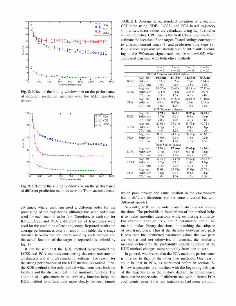
The similarity based prediction method presented hereis categorized as a non-parametric method. Therefore, theperformance of the mentioned methods depends on the sizeof the history of reference trajectories used for prediction.We performed some experiments and observed that as thesize of the history of reference trajectories exceeds 1000trajectories, the increases in size does not significantly affectthe performance of the prediction method (see Fig. 8 and9). Therefore, the trajectory history was maintained as asliding window with the size of 1000. This means that ateach time step, in order to predict the trajectory of a newtarget, only the trajectories of the previous 1000 targets areused. In this manner, the prediction time for each trajectoryremains manageable for the large datasets (MIT and TrainStation).

The performances of the KDE, LCSS, and PCA predictionmethods are reported in Table I. Each method was run

0 200 400 600 800 1000 1200 1400 1600Sliding window size

10

15

20

25

30

35

40

45

50

55Err

or

(p)

PCAKDELCSS

Fig. 8: Effect of the sliding window size on the performanceof different prediction methods over the MIT trajectorydataset.

0 200 400 600 800 1000 1200 1400 1600Sliding window size

0

20

40

60

80

100

Err

or

(p)

PCAKDELCSS

Fig. 9: Effect of the sliding window size on the performanceof different prediction methods over the Train station dataset.

30 times, where each run used a different order for theprocessing of the trajectories, although the same order wasused for each method to be fair. Therefore, at each run forKDE, LCSS, and PCA a different set of trajectories wereused for the prediction of each trajectory. Reported results areaverage performances over 30 runs. In this table, the averagedistance between the prediction made by each method andthe actual location of the target is reported (as defined byEq. 1).

It can be seen that the KDE method outperformed theLCSS and PCA methods considering the error measure onall datasets and with all simulation settings. The reason forthe strong performance of the KDE method is twofold. First,the KDE method is the only method which considers both thelocation and the displacement in the similarity function. Theaddition of displacement in the similarly function helps theKDE method to differentiate more clearly between targets

TABLE I: Average error, standard deviation of error, andCPU time using KDE-, LCSS- and PCA-based trajectorysimilarities. Error values are calculated using Eq. 1, smallervalues are better. CPU time is the Wall Clock time needed toestimate the location of one target. Tested settings correspondto different current times (t) and prediction time steps (s).Bold values represent statistically significant results accord-ing to the Wilcoxon signed-rank test (p-value=0.05) whencompared pairwise with both other methods.

t = 5 t = 5 t = 15 t = 15s = 5 s = 20 s = 5 s = 20

ULaval Campus simulated dataset

KDEAvg. err. 10.04 m 44.18 m 11.45 m 35.52 mStdev. err. 0.27 m 1.2 m 0.3 m 0.74 mCPU time 4.0 s 4.5 s 3.5 s 3.5 s

LCSSAvg. err. 15.62 m 53.66 m 31.18 m 67.22 mStdev. err. 0.34 m 1.2 m 0.38 m .92 mCPU time 1.5 s 1.5 s 4.0 s 4.0 s

PCAAvg. err. 15.7 m 55.22 m 21.04 m 51.16 mStdev. err. 0.4 m 0.87 m 0.6 m 1.05 mCPU time 1.0 s 1.0 s 1.5 s 1.5 s

MIT Trajectory dataset

KDEAvg. err. 11.91 p 26.0 p 10.95 p 24.10 pStdev. err. 0.7 p 0.6 p 0.4 p 0.6 pCPU time 4.0 s 4.0 s 4.0 s 3.8 s

LCSSAvg. err. 27.62 p 37.61 p 28.73 p 40.72 pStdev. err. 1.2 p 1.8 p 0.9 p 0.6 pCPU time 1.4 s 1.5 s 4.4 s 4.3 s

PCAAvg. err. 31.58 p 44.41 p 36.12 p 48.62 pStdev. err. 0.9 p 0.6 p 1.8 p 0.5 pCPU time 1.0 s 1.0 s 1.5 s 1.5 s

Train Station dataset

KDEAvg. err. 12.99 p 17.86 p 12.66 p 18.06 pStdev. err. 0.4 p 0.51 p 0.41 p 0.6 pCPU time 4.5 s 4.9 s 4.8 s 4.7 s

LCSSAvg. err. 30.42 p 31.17 p 34.52 p 36.42 pStdev. err. 0.2 p 0.1 p 1.4 p 1.0 pCPU time 2.4 s 2.3 s 4.0 s 4.1 s

PCAAvg. err. 52.01 p 55.98 p 53.0 p 57.71 pStdev. err. 0.6 p 0.6 p 0.4 p 0.8 pCPU time 1.0 s 1.0 s 1.5 s 1.5 s

which pass through the same location in the environmentbut in different directions (or the same direction but withdifferent speeds).

Secondly, KDE is the only probabilistic method amongthe three. The probabilistic foundations of the method helpsit to make smoother decisions while estimating similarity.For example, through its ε and δ parameters, the LCSSmethod makes binary decisions in matching the subpartsof two trajectories. Thus if the distance between two partsis less than the mentioned parameter values the two partsare similar and not otherwise. In contrast, the similaritymeasure defined by the probability density function of theKDE method changes more smoothly from one to zero.

In general, we observe that the PCA method’s performanceis inferior to that of the other two methods. One reasoncould be that in PCA, as mentioned before in section IV-E, new trajectories are matched with the beginning sub-partof the trajectories in the history dataset. In consequence,there can be trajectories of different size with different PCAcoefficients, even if the two trajectories had some common

sub-parts.Considering the computational demand, PCA is the least

computationally expensive method. The computational costof the LCSS method depends on the prediction times. Forthe smaller prediction times (t = 5), the computationalcost is comparable with the PCA method, but for the largerprediction times (t = 15), the computation time is similar tothat of the KDE method.

In all settings, increasing the prediction time step from(s = 5) to (s = 20) has increased the expected error,which is reasonable – predicting further into the futureincreases the uncertainty. The interesting point is that foreach dataset, increasing the prediction time step has roughlythe same effect over different methods (i.e., the increase ofthe expected error is comparable for different methods overone dataset). This suggests that the properties of the dataset(i.e., nature of the trajectories composing the dataset) has amore significant impact over long term prediction accuracythan the prediction methods. For example, the simulateddataset has the largest drop in performance between theshort (s = 5) and long (s = 20) prediction time steps.This could be related to the fact that the targets changedirection more frequently in the simulated dataset than inthe other two datasets. In this dataset, targets share part oftheir trajectory with many other targets, unlike the other twodatasets, where each target usually keeps the initial directionof its movement.

Another interesting observation is that the increase of theprediction time from (t = 5) to (t = 15) has decreasedthe performance of the LCSS and PCA algorithms, but inmost cases improved the performance of the KDE algorithm.When increasing the prediction time, each algorithm hasmore information to process. If done properly, as in the caseof KDE, this leads to a decrease in the number of falsepositives (wrongfully considering two trajectories similar,while they are not). Otherwise, as in LCSS and PCA, thisonly increases the confusion of the overall algorithm, andreduces the performance of the system.

Another explanation is that KDE has a mechanism todeal with missing data points by taking into account theuncertainty (i.e., variance) over the estimated location ofthe target, while the two other methods rely only in theinterpolated positions. That could be the reason that theperformance of different methods is closer on the simulateddataset (in which there is no unobserved trajectory) comparedto the two other real datasets where there are unobservedpoints.

VI. CONCLUSION

This paper has presented a model to measure similaritybetween trajectories of targets moving inside an environmentusing the kernel density estimation. The effectiveness ofthe proposed model is shown in the trajectory predictionproblem. The goal in trajectory prediction is to estimate thefuture location of a new target moving in an environmentusing the history of previous trajectories that were observedso far in the same environment.

For experiments conducted on one simulated and tworeal datasets, the proposed model was compared with twoother commonly used methods, namely PCA and LCSS,for measuring the similarity between trajectories. Resultsshowed that although the proposed approach is slightly moreexpensive in terms of computation time, it outperformed bothof the other methods over all tested datasets and simulationsettings. The strong performance of the method is related toits probabilistic nature and consideration of the displacementin the similarity function.

ACKNOWLEDGEMENTS

This work was supported through funds from NSERC(Canada) and access to computational resources of CalculQuebec / Compute Canada. We thank Annette Schwerdtfegerfor proofreading this manuscript.

REFERENCES

[1] Faisal I Bashir, Ashfaq A Khokhar, and Dan Schonfeld. Segmentedtrajectory based indexing and retrieval of video data. In Proc. of theIntl Conf. on Image Processing (ICIP 2003), volume 2, pages 623–626, 2003.

[2] Maren Bennewitz, Wolfram Burgard, and Sebastian Thrun. Learningmotion patterns of persons for mobile service robots. In Proc. of theIEEE Intl Conf. on Robotics and Automation (ICRA 2002), volume 4,pages 3601–3606, 2002.

[3] Neil J Gordon, David J Salmond, and Adrian FM Smith. Novelapproach to nonlinear/non-gaussian bayesian state estimation. IEEProceedings F (Radar and Signal Processing), 140:107–113, 1993.

[4] Rudolph Emil Kalman. A new approach to linear filtering andprediction problems. Journal of Basic Engineering, 82(1):35–45, 1960.

[5] Eamonn J Keogh and Michael J Pazzani. Scaling up dynamic timewarping for datamining applications. In Proc. of ACM Intl Conf. onKnowledge Discovery and Data Mining (KDD 2000), pages 285–289,2000.

[6] Markus Kuderer, Henrik Kretzschmar, Christoph Sprunk, and WolframBurgard. Feature-based prediction of trajectories for socially compliantnavigation. In Robotics: Science and Systems, 2012.

[7] Cynthia Sung, Dan Feldman, and Daniela Rus. Trajectory clusteringfor motion prediction. In Proc. of the IEEE/RSJ Intl Conf. onIntelligent Robots and Systems (IROS 2012), pages 1547–1552, 2012.

[8] Dizan Vasquez, Thierry Fraichard, and Christian Laugier. Growinghidden Markov models: An incremental tool for learning and pre-dicting human and vehicle motion. International Journal of RoboticsResearch, 28(11-12):1486–1506, 2009.

[9] Michail Vlachos, George Kollios, and Dimitrios Gunopulos. Discov-ering similar multidimensional trajectories. In Proc. of the Intl Conf.on Data Engineering (ICDE 2002), pages 673–684, 2002.

[10] Xiaogang Wang, Eric Grimson, Gee-Wah Ng, and Keng Teck Ma. Tra-jectory analysis and semantic region modeling using a nonparametricbayesian model. In Proc. of the IEEE Conf. on Computer Vision andPattern Recognition (CVPR 2008), 2008.

[11] Zhang Zhang, Kaiqi Huang, and Tieniu Tan. Comparison of similaritymeasures for trajectory clustering in outdoor surveillance scenes. InProc. of the Intl Conf. on Pattern Recognition (ICPR 2006), volume 3,pages 1135–1138, 2006.

[12] Bolei Zhou, Xiaogang Wang, and Xiaoou Tang. Understandingcollective crowd behaviors: Learning a mixture model of dynamicpedestrian-agents. In Proc. of the IEEE Conf. on Computer Visionand Pattern Recognition (CVPR 2012), pages 2871–2878, 2012.

[13] Brian D. Ziebart, Nathan Ratliff, Garratt Gallagher, Christoph Mertz,Kevin Peterson, J. Andrew Bagnell, Martial Hebert, Anind K. Dey,and Siddhartha Srinivasa. Planning-based prediction for pedestrians.In Proceedings of the 2009 IEEE/RSJ International Conference onIntelligent Robots and Systems, IROS’09, pages 3931–3936, 2009.