Kernel Adaptive Filtering - Computational … · Outline 1. Optimal adaptive signal processing...

Kernel Adaptive Filtering

Jose C. Principe and Weifeng Liu

Computational NeuroEngineering Laboratory (CNEL) University of Florida

[email protected], [email protected]

Acknowledgments

Dr. Badong Chen Tsinghua University and Post Doc CNEL NSF ECS – 0300340 and 0601271 (Neuroengineering program)

Outline

1. Optimal adaptive signal processing fundamentals Learning strategy Linear adaptive filters 2. Least-mean-square in kernel space Well-posedness analysis of KLMS 3. Affine projection algorithms in kernel space 4. Extended recursive least squares in kernel space 5. Active learning in kernel adaptive filtering

Wiley Book (2010)

Papers are available at www.cnel.ufl.edu

Part 1: Optimal adaptive signal processing fundamentals

Machine Learning Problem Definition for Optimal System Design

Assumption: Examples are drawn independently from an unknown probability distribution P(u, y) that represents the rules of Nature. Expected Risk: Find f∗ that minimizes R(f) among all functions. But we use a mapper class F and in general The best we can have is that minimizes R(f). P(u, y) is also unknown by definition. Empirical Risk: Instead we compute that minimizes Rn(f). Vapnik-Chervonenkis theory tells us when this will work, but the optimization is computationally costly. Exact estimation of fN is done thru optimization.

∫= ),()),(()( yudPyufLfR

∑=i

iiN yufLNfR )),((/1)(ˆ

Ff ∉*

FfF ∈*

FfN ∈

Machine Learning Strategy

The optimality conditions in learning and optimization theories are mathematically driven:

Learning theory favors cost functions that ensure a fast estimation rate when the number of examples increases (small estimation error bound). Optimization theory favors super-linear algorithms (small approximation error bound)

What about the computational cost of these optimal solutions, in particular when the data sets are huge? Estimation error will be small, but can not afford super linear solutions:

Algorithmic complexity should be as close as possible to O(N).

Statistic Signal Processing Adaptive Filtering Perspective

Adaptive filtering also seeks optimal models for time series. The linear model is well understood and so widely applied. Optimal linear filtering is regression in functional spaces, where the user controls the size of the space by choosing the model order. Problems are fourfold:

Application conditions may be non stationary, i.e. the model must be continuously adapting to track changes. In many important applications data arrives in real time, one sample at a time, so on-line learning methods are necessary. Optimal algorithms must obey physical constrains, FLOPS, memory, response time, battery power. Unclear how to go beyond the linear model.

Although the optimalilty problem is the same as in machine learning, constraints make the computational problem different.

Since achievable solutions are never optimal (non-reachable set of functions, empirical risk), goal should be to get quickly to the neighborhood of the optimal solution to save computation. The two types of errors are

Approximation error Estimation error

But fN is difficult to obtain, so why not create a third error (Optimization Error) to approximate the optimal solution

provided it is computationally simpler to obtain. So the problem is to find F, N and ρ for each application.

Machine Learning+Statistical SP Change the Design Strategy

)()(

)()()()(*

***

FN

FN

fRfR

fRfRfRfR

−+

+−=−

ρ=− )~()( NN fRfR

Leon Bottou: The Tradeoffs of Large Scale Learning, NIPS 2007 tutorial

Learning Strategy in Biology

In Biology optimality is stated in relative terms: the best possible response within a fixed time and with the available (finite) resources. Biological learning shares both constraints of small and large learning theory problems, because it is limited by the number of samples and also by the computation time. Design strategies for optimal signal processing are similar to the biological framework than to the machine learning framework. What matters is “how much the error decreases per sample for a fixed memory/ flop cost” It is therefore no surprise that the most successful algorithm in adaptive signal processing is the least mean square algorithm (LMS) which never reaches the optimal solution, but is O(L) and tracks continuously the optimal solution!

Extensions to Nonlinear Systems

Many algorithms exist to solve the on-line linear regression problem:

LMS stochastic gradient descent LMS-Newton handles eigenvalue spread, but is expensive Recursive Least Squares (RLS) tracks the optimal solution with the available data.

Nonlinear solutions either append nonlinearities to linear filters (not optimal) or require the availability of all data (Volterra, neural networks) and are not practical. Kernel based methods offers a very interesting alternative to neural networks.

Provided that the adaptation algorithm is written as an inner product, one can take advantage of the “kernel trick”. Nonlinear filters in the input space are obtained. The primary advantage of doing gradient descent learning in RKHS is that the performance surface is still quadratic, so there are no local minima, while the filter now is nonlinear in the input space.

Adaptive Filtering Fundamentals

Adaptive System

Output

On-Line Learning for Linear Filters

The current estimate is computed in terms of the previous estimate, , as: ei is the model prediction error arising from the use of wi-1 and Gi is a

Gain term

iw

1i i i iw w G e−= +1iw −

Transversal filter

Adaptive weight-control mechanism

iwiu ( )y i

Σ

( )d i

-

+

( )e i

Notation:

wi weight estimate at time i (vector) (dim = l)

ui input at time i (vector)

e(i) estimation error at time i (scalar)

d(i) desired response at time i (scalar)

ei estimation error at iteration i (vector)

di desired response at iteration i (vector)

Gi capital letter matrix


sizestep

ieEJ

wwmEilJww

ii

iii

η

η

)]([

*][

2

1

=

=∇−= −

W1

W2

-1 -0.5 0 0.5 1 1.5 2 2.5 30

0.5

1

1.5

2

2.5

3

3.5

4ContourMEEFP-MEE

11

1 −−

− ∇−= iii JHww η


Gradient descent learning for linear mappers has also great properties

It accepts an unbiased sample by sample estimator that is easy to compute (O(L)), leading to the famous LMS algorithm. The LMS is a robust estimator ( ) algorithm. For small stepsizes, the visited points during adaptation always belong to the input data manifold (dimension L), since algorithm always move in the opposite direction of the gradient.

)(1 ieuww iii η+= −

∞H

On-Line Learning for Non-Linear Filters?

Can we generalize to nonlinear models?

and create incrementally the nonlinear mapping?

Ty w u= ( )y f u=

Universal function approximator

Adaptive weight-control mechanism

ifiu ( )y i

Σ

( )d i

-

+

( )e i

1i i i iw w G e−= +

iiii eGff += −1

Part 2: Least-mean-squares in kernel space

Non-Linear Methods - Traditional (Fixed topologies)

Hammerstein and Wiener models An explicit nonlinearity followed (preceded) by a linear filter Nonlinearity is problem dependent Do not possess universal approximation property

Multi-layer perceptrons (MLPs) with back-propagation Non-convex optimization Local minima

Least-mean-square for radial basis function (RBF) networks Non-convex optimization for adjustment of centers Local minima

Volterra models, Recurrent Networks, etc

Non-linear Methods with kernels

Universal approximation property (kernel dependent) Convex optimization (no local minima) Still easy to compute (kernel trick) But require regularization Sequential (On-line) Learning with Kernels

(Platt 1991) Resource-allocating networks

Heuristic No convergence and well-posedness analysis

(Frieb 1999) Kernel adaline Formulated in a batch mode well-posedness not guaranteed

(Kivinen 2004) Regularized kernel LMS with explicit regularization Solution is usually biased

(Engel 2004) Kernel Recursive Least-Squares (Vaerenbergh 2006) Sliding-window kernel recursive least-squares

Neural Networks versus Kernel Filters

ANNs Kernel filters

Universal Approximators YES YES Convex Optimization NO YES Model Topology grows with data NO YES

Require Explicit Regularization NO YES/NO (KLMS)

Online Learning YES YES

Computational Complexity LOW MEDIUM

ANNs are semi-parametric, nonlinear approximators Kernel filters are non-parametric, nonlinear approximators

Kernel Methods

)()()(1

0ninxwny

L

ii xwT=−= ∑

−

=

Kernel filters operate in a very special Hilbert space of functions called a Reproducing Kernel Hilbert Space (RKHS). A RKHS is an Hilbert space where all function evaluations are finite Operating with functions seems complicated and it is! But it becomes much easier in RKHS if we restrict the computation to inner products. Most linear algorithms can be expressed as inner products. Remember the FIR

Kernel Methods

Moore-Aronszajn theorem Every symmetric positive definite function of two real variables in E κ(x,y) defines a unique Reproducing Kernel Hilbert Space (RKHS).

Mercer’s theorem Let κ(x,y) be symmetric positive definite. The kernel can be expanded in the series Construct the transform as Inner product

( ) ( ) ( )x y x yϕ ϕ κ, = ,

1( , ) ( ) ( )

m

i i ii

x y x yκ λϕ ϕ=

= ∑

1 1 2 2( ) [ ( ), ( ),..., ( )]Tm mx x x xϕ λ ϕ λ ϕ λ ϕ=

)exp(),( 2yxhyx −−=κκ

κκ

HxfxfHfExIIHxExI

>=<∈∀∈∀∈∈∀

)(.,,)(,)()(.,)(

Kernel methods

Mate L., Hilbert Space Methods in Science and Engineering, A. Hildger, 1989 Berlinet A., and Thomas-Agnan C., “Reproducing kernel Hilbert Spaces in probaability and Statistics, Kluwer 2004

Basic idea of on-line kernel filtering

Transform data into a high dimensional feature space Construct a linear model in the feature space F Adapt iteratively parameters with gradient information Compute the output Universal approximation theorem

For the Gaussian kernel and a sufficient large mi, fi(u) can approximate any continuous input-output mapping arbitrarily close in the Lp norm.

: ( )i iuϕ ϕ=

1( ) , ( ) ( , )

im

i i F j jj

f u u a u cϕ κ=

= ⟨Ω ⟩ = ∑

, ( ) Fy uϕ= ⟨Ω ⟩

iii J∇+Ω=Ω − η1

Growing network structure

u

φ(u)

Ω+

y

1 ( ) ( )i i ie i uη ϕ−Ω = Ω +

1 ( ) ( , )i i if f e i uη κ−= + ⋅

+

a1

a2

ami-1

ami

c1

c2

cmi-1

cmi

yu

Kernel Least-Mean-Square (KLMS) Least-mean-square Transform data into a high dimensional feature space F

RBF Centers are the samples, and Weights are the errors!

011 )()()( wuwidieieuww iTiiii −− −=+= η

: ( )i iuϕ ϕ=

0

1

1

0( ) ( ) , ( )

( ) ( )i i F

i i i

e i d i uu e i

ϕηϕ

−

−

Ω == − ⟨Ω ⟩

Ω = Ω +

1( ) ( )

i

i jj

e j uη ϕ=

Ω = ∑

1( ) , ( ) ( ) ( , )

i

i i F jj

f u u e j u uϕ η κ=

= ⟨Ω ⟩ = ∑

0

0 1

1 0 1 1 1

1 2

1 1 2

1 1 2

2 1 2

1 1 2 2

0(1) (1) , ( ) (1)

( ) (1) ( )(2) (2) , ( )

(2) ( ), ( )(2) ( , )

( ) (2)( ) ( )

...

F

F

F

e d u du e a u

e d ud a u ud a u u

u ea u a u

ϕηϕ ϕ

ϕϕ ϕ

κηϕ

ϕ ϕ

Ω == − ⟨Ω ⟩ =

Ω = Ω + == − ⟨Ω ⟩= − ⟨ ⟩= −

Ω = Ω += +

Kernel Least-Mean-Square (KLMS)

),.)(()(

))(()()(

))(),(()())((

),.)(()(

1

1

1

11

1

11

iieff

ifidie

ijjeif

jjef

ii

i

i

ji

i

ji

u

u

uuu

u

κη

κη

κη

+=

−=

=

=

−

−

−

=−

−

=−

∑

∑

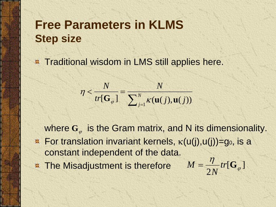
Free Parameters in KLMS Step size

Traditional wisdom in LMS still applies here.

where is the Gram matrix, and N its dimensionality. For translation invariant kernels, κ(u(j),u(j))=g0, is a constant independent of the data. The Misadjustment is therefore

ϕG

][2 ϕη GtrN

M =

∑ =

=< N

jjj

Ntr

N

1))(),((][ uuG κ

ηϕ

Free Parameters in KLMS Rule of Thumb for h

Although KLMS is not kernel density estimation, these rules of thumb still provide a starting point. Silverman’s rule can be applied

where σ is the input data s.d., R is the interquartile, N is the number of samples and L is the dimension. Alternatively: take a look at the dynamic range of the data, assume it uniformly distributed and select h to put 10 samples in 3 σ.

)5/(134.1/,min06.1 LNRh −= σ

Free Parameters in KLMS Kernel Design

The Kernel defines the inner product in RKHS Any positive definite function (Gaussian, polynomial, Laplacian, etc.), but we should choose a kernel that yields a class of functions that allows universal approximation. A strictly positive definite function is preferred because it will yield universal mappers (Gaussian, Laplacian).

See Sriperumbudur et al, On the Relation Between Universality, Characteristic Kernels and RKHS Embedding of Measures, AISTATS 2010

Free Parameters in KLMS Kernel Design

Estimate and minimize the generalization error, e.g. cross validation Establish and minimize a generalization error upper bound, e.g. VC dimension Estimate and maximize the posterior probability of the model given the data using Bayesian inference

Free Parameters in KLMS Bayesian model selection

The posterior probability of a Model H (kernel and parameters θ) given the data is

where d is the desired output and U is the input vector. This is hardly ever done for the kernel function, but it

can be applied to θ and leads to Bayesian principles to adapt the kernel parameters.

)|()(),|(),|(

UdUdUdp

HpHpHp iii =

Free Parameters in KLMS Maximal marginal likelihood

)]2log(2log21)(21[)( 212 πσσθ

NxamHJ nnT

i −+−+−= − IGdIGd

Sparsification

Filter size increases linearly with samples! If RKHS is compact and the environment stationary, we see that there is no need to keep increasing the filter size. Issue is that we would like to implement it on-line! Two ways to cope with growth:

Novelty Criterion Approximate Linear Dependency

First is very simple and intuitive to implement.

Sparsification Novelty Criterion

Present dictionary is . When a new data pair arrives (u(i+1),d(i+1)). First compute the distance to the present dictionary If smaller than threshold δ1 do not create new center Otherwise see if the prediction error is larger than δ2 to augment the dictionary. δ1 ~ 0.1 kernel size and δ2 ~ sqrt of MSE

imjjciC

1)(

==

jCcciudis

j

−+=∈

)1(min

Sparsification Approximate Linear Dependency

Engel proposed to estimate the distance to the linear span of the centers, i.e. compute

Which can be estimated by

Only increase dictionary if dis larger than threshold Complexity is O(m2) Easy to estimate in KRLS (dis~r(i+1)) Can simplify the sum to the nearest center, and it defaults to NC

)())1((min jCc jbcbiudis

j∑ ∈∨

−+= ϕϕ

)1()()1())1(),1(( 12 ++−++= − iiiiidis T hGhuuκ

)())1((min, jCcb

ciudisj

ϕϕ −+=∈∨

KLMS- Mackey-Glass Prediction

30)(1)(2.0)(1.0)( 10 =

−+−

+−= τττ

txtxtxtx

LMS η=0.2 KLMS a=1, η=0.2

Regularization worsens performance

Performance Growth tradeoff

δ1=0.1, δ2=0.05 η=0.1, a=1

KLMS- Nonlinear channel equalization

1( ) , ( ) ( ) ( , )

i

i i F jj

f u u e j u uϕ η κ=

= ⟨Ω ⟩ = ∑

( )mi i

mi

c ua e iη

←←

+

a1

a2

ami-1

ami

c1

c2

cmi-1

cmi

yu

10.5t t tz s s −= + 20.9t t tr z z nσ= − +st rt

Nonlinear channel equalization

Algorithms Linear LMS (η=0.005) KLMS (η=0.1) (NO REGULARIZATION)

RN (REGULARIZED λ=1)

BER (σ = .1) 0.162±0.014 0.020±0.012 0.008±0.001

BER (σ = .4) 0.177±0.012 0.058±0.008 0.046±0.003

BER (σ = .8) 0.218±0.012 0.130±0.010 0.118±0.004

Algorithms Linear LMS KLMS RN

Computation (training) O(l) O(i) O(i3)

Memory (training) O(l) O(i) O(i2)

Computation (test) O(l) O(i) O(i)

Memory (test) O(l) O(i) O(i)

2( , ) exp( 0.1 || || )i j i ju u u uκ = − −

Why don’t we need to explicitly regularize the KLMS?

Self-regularization property of KLMS Assume the data model then for any unknown vector the following inequality holds

As long as the matrix is positive definite. So H∞ robustness And is upper bounded

The solution norm of KLMS is always upper bounded i.e. the algorithm is well posed in the sense of Hadamard.

( ) ( ) ( )oid i v iϕ= Ω +

2 2 21|| || (|| || 2 || || )o

N vσ η ηΩ < Ω +

2 1 2 2|| || || || 2 || ||oe vη −< Ω +

21

11 2 21

| ( ) ( ) |1, 1, 2,...,

|| || | ( ) |

i

jioj

e j v jfor all i N

v jη=

−−=

−< =

Ω +

∑∑

σ1 is the largest eigenvalue of Gφ

Liu W., Pokarel P., Principe J., “The Kernel LMS Algorithm”, IEEE Trans. Signal Processing, Vol 56, # 2, 543 – 554, 2008.

)()( 1 TiiI ϕϕη −−

0Ω

)(nΩ

Regularization Techniques

Learning from finite data is ill-posed and a priori information to enforce Smoothness is needed. The key is to constrain the solution norm

In Least Squares constraining the norm yields

In Bayesian modeling, the norm is the prior. (Gaussian process)

In statistical learning theory, the norm is associated with the model capacity and hence the confidence of uniform convergence! (VC dimension and structural risk minimization)

2 2

1

1( ) ( ( ) ) || ||N

Ti

iJ d i

Nϕ λ

=

Ω = − Ω + Ω∑Gaussian

distributed prior

2 2

1

1( ) ( ( ) ) , subject to || ||N

Ti

iJ d i C

Nϕ

=

Ω = − Ω Ω <∑

Norm constraint

Tikhonov Regularization

12 2

1

( ,..., ,0,...,0) Tr

r

s sPdiag Q ds sλ λ

Ω =+ +

1 2 , ,..., rS diag s s s=Singular value

Notice that if λ = 0, when sr is very small, sr/(sr2+ λ) = 1/sr → ∞.

However if λ > 0, when sr is very small, sr/(sr2+ λ) = sr/ λ → 0.

In numerical analysis the method is to constrain the condition number of the solution matrix (or its eigenvalues) The singular value decomposition of Φ can be written The pseudo inverse to estimate Ω in is

which can be still ill-posed (very small sr). Tikhonov regularized the

least square solution to penalize the solution norm to yield

TQS

PΦ

=

000

)()()( 0 iiid T νϕ +Ω=

dQP TrPI ssdiag ]0....0,,...,[ 11

1−−=Ω

2d Ω+Ω−=Ω λTJ Φ)(

Tikhonov and KLMS For finite data and using small stepsize theory: Denote Assume the correlation matrix is singular, and

From LMS it is known that Define so and

2 2 2min min0[| ( ) | ] (1 ) (| ( ) | )

2 2i

i nn n

J JE n nη ηε ης ε

ης ης= + − −

− −

1 1... ... 0k k mς ς ς ς+≥ ≥ > = = =


TxR P P= Λ( ) m

i iu Rϕ ϕ= ∈1

1 NT

i ii

RNϕ ϕ ϕ

=

= ∑

)0()1()]([ ni

nn iE εηςε −=

∑ ==Ω−Ω

m

n nn Pii1

0 )()( ε

jj

M

j

ijjj

M

j

ijiE PP 0

11

0 ])1(1[)0()1()]([ Ω−−=−+Ω=Ω ∑∑==

ηςεης 0)0(0)0( jj Ω−==Ω ε

20

1

202 )()]([ Ω=Ω≤Ω ∑=

M

jjiE max/1 ςη ≤

Tikhonov and KLMS In the worst case, substitute the optimal weight by the pseudo inverse Regularization function for finite N in KLMS No regularization Tikhonov

PCA

2 2 1[ /( )]n n ns s sλ −+ ⋅

1 if th0 if th

n n

n

s ss

− >

≤

1ns −

2 1[1 (1 / ) ]Nn ns N sη −− − ⋅

0 0.5 1 1.5 2

0

0.2

0.4

0.6

0.8

1

singular value

reg-

func

tion

KLMSTikhonovTruncated SVD

The stepsize and N control the reg-function in KLMS.

Liu W., Principe J. The Well-posedness Analysis of the Kernel Adaline, Proc WCCI, Hong-Kong, 2008

dQP Tr

ir

i ssdiagiE ]0....0,))1(1(,...,))1(1[()]([ 1111

−− −−−−=Ω ηςης

The minimum norm initialization for KLMS

The initialization gives the minimum possible norm solution.

00 =Ω

1

mi n nn

c P=

Ω = ∑

2 2 21 1

|| || || || || ||k mi n nn n k

c c= = +

Ω = +∑ ∑

0 2 4-1

0

1

2

3

4

5

1

1

... 0... 0

k

k m

ς ςς ς+

≥ ≥ >= = =


KLMS and the Data Space

KLMS search is insensitive to the 0-eigenvalue directions

So if , and

The 0-eigenvalue directions do not affect the MSE

2 2min minmin 1 1

( ) (| (0) | )(1 )2 2

m m in n n nn n

J JJ i J η ης ς ε ης

= == + + − −∑ ∑

KLMS only finds solutions on the data subspace! It does not care about the null space!


2( ) [| | ]TiJ i E d ϕ= − Ω

)0()1()]([ ni

nn iE εηςε −=

2 2 2min min0[| ( ) | ] (1 ) (| ( ) | )

2 2i

i nn n

J JE n nη ηε ης ε

ης ης= + − −

− −0nς = )0()]([ nn iE εε =

22 )0(])([ nn iE εε =

Energy Conservation Relation

Energy conservation in RKHS Upper bound on step size for mean square convergence

Steady-state mean square performance

The fundamental energy conservation relation holds in RKHS!

Chen B., Zhao S., Zhu P., Principe J. Mean Square Convergence Analysis of the Kernel Least Mean Square Algorithm, submitted to IEEE Trans. Signal Processing

( ) ( )

222 2 ( )( )( ) ( 1)( ), ( ) ( ), ( )

pa e ie ii ii i i iκ κ

+ = − + Ω Ωu u u uF F

2*

2* 2

2

v

E

Eη

σ

≤

+

Ω

Ω

F

F

22lim ( )

2v

aiE e i ησ

η→∞ = −

0.2 0.4 0.6 0.8 10

0.002

0.004

0.006

0.008

0.01

0.012

stepsize ηE

MS

E

simulationtheory

Effects of Kernel Size

0.5 1 1.5 20

1

2

3

4

5

6

7

8

x 10-3

kernel size σ

EM

SE

simulationtheory

0 200 400 600 800 10000

0.1

0.2

0.3

0.4

0.5

0.6

0.7

0.8

iteration

EM

SE

σ = 0.2σ = 1.0σ = 20

Kernel size affects the convergence speed! (How to choose a suitable kernel size is still an open problem)

However, it does not affect the final misadjustment! (universal

approximation with infinite samples)

Part 3: Affine projection algorithms in kernel space

The big picture for gradient based learning

APA Newton APA

Leaky APA

LMS Normalized LMS

Leaky LMS

K=1

K=1

K=1

Adaline RLSK=

i

K=i

Extended RLS

weighted RLS

Frieb , 1999

Kivinen 2004

Engel, 2004 We have kernelized versions of all The EXT RLS is a model with states

Liu W., Principe J., “Kernel Affine Projection Algorithms”, European J. of Signal Processing, ID 784292, 2008.

Affine projection algorithms

Solve which yields There are several ways to approximate this solution iteratively using

Gradient Descent Method Newton’s recursion

LMS uses a stochastic gradient that approximates Affine projection algorithms (APA) utilize better approximations Therefore APA is a family of online gradient based algorithms of intermediate complexity between the LMS and RLS.

2)(min uww T

wdEJ −= du

-1u rRw =0

)]1([)1()()0( −+−= iii wR-rwww uduη

)]1([)()1()()0( 1 −++−= − iii wR-rIRwww uduu εη

)()(ˆ)()(ˆ iidii T uruuR duu ==


APA are of the general form

Gradient

Newton Notice that So

TLxK idKidiiKii )](),...,1([)()](),...,1([)( +−=+−= duuU

)()(1ˆ)()(1ˆ iiK

iiK

T dUrUUR duu ==

)]1()()()()1()()0( −+−= iiiiii T wU-[dUwww η

)]1()()()[())()(()1()( 1 −++−= − iiiiiiii TT wU-dUIUUww εη

11 ))()()(()())()(( −− +=+ IUUUUIUU εε iiiiii TT

)]1()()([])()()[()1()( 1 −++−= − iiiiiiii TT wU-dIUUUww εη


If a regularized cost function is preferred The gradient method becomes

Newton Or

)]1()()()()1()1()()0( −+−−= iiiiii T wU-[dUwww ηηλ

)()())()(()1()1()( 1 iiiiii T dUIUUww −++−−= εηηλ

22)(min wuww λ+−= T

wdEJ

)(])()()[()1()1()( 1 iiiiii T dIUUUww −++−−= εηηλ

Kernel Affine Projection Algorithms

KAPA 1,2 use the least squares cost, while KAPA 3,4 are regularized KAPA 1,3 use gradient descent and KAPA 2,4 use Newton update Note that KAPA 4 does not require the calculation of the error by

rewriting the error with the matrix inversion lemma and using the kernel trick

Note that one does not have access to the weights, so need recursion as in KLMS.

Care must be taken to minimize computations.

Ω≡wQ(i)

KAPA-1

1( ) , ( ) ( , )

i

i i F j jj

f u u a u uϕ κ=

= ⟨Ω ⟩ = ∑

1 1

1 1

( )( 1)

( 1)

mi i

mi i

mi mi i

mi K mi K i

c ua e ia a e i

a a e i K

ηη

η

− −

− + − +

←←

← + −

← + − +

+

a1

a2

ami-1

ami

c1

c2

cmi-1

cmi

yu

KAPA-1

)(),1()(

,...,1)1()(

1,....,11);()1()();()(

),.)(();(11

1

iiCiCKijii

iKjjieiiiiei

jjieff

jj

jj

i

i

Kjii

uaaaa

a

u

−=

−=−=

−+−=+−==

+= ∑+−=

−

ηη

κη

Error reusing to save computation

For KAPA-1, KAPA-2, and KAPA-3 To calculate K errors is expensive (kernel evaluations)

K times computations? No, save previous errors and use them

1( ) ( ) , ( 1 )Ti k ie k d k i K k iϕ −= − Ω − + ≤ ≤

1 1

1

1

( ) ( ) ( ) ( )

( ( ) )

( )

( ) ( ) .

T Ti k i k i i i

T Tk i k i i

Ti k i i

iT

i i k jj i K

e k d k d k e

d k e

e k e

e k e j

ϕ ϕ η

ϕ ηϕ

ηϕ

η ϕ ϕ

+ −

−

= − +

= − Ω = − Ω + Φ

= − Ω + Φ

= + Φ

= + ∑

Still needs which requires i kernel evals,

So O(i+K2)

( 1)ie i +

KAPA-4: Smoothed Newton’s method. There is no need to compute the error The topology can still be put in the same RBF framework. Efficient ways to compute the inverse are necessary. The sliding window computation yields a complexity of O(K2)

KAPA-4

1 1[ , ,..., ]

[ ( ), ( 1),..., ( 1)]i i i i K

Tid d i d i d i K

ϕ ϕ ϕ− − +Φ =

= − − +

)(])()()[()1()1()( 1 iiiiii T dIww −+ΦΦΦ+−−= ληηλ

How to invert the K-by-K matrix and avoid O(K3)?

KAPA-4

( )Ti iIε + Φ Φ

)())(()(~11)1()1()(

11)(~)1()1()(

)(~)(

1 iii

KikiiikKikdii

ikidi

kk

kk

k

dIGd

aaaa

a

−+=

+−≤≤−−=−≤≤+−+−−=

==

λ

ηηη

η

Ti i iGr = Φ Φ

Sliding window Gram matrix inversion

1 1[ , ,..., ]i i i i Kϕ ϕ ϕ− − +Φ =

T

ia b

Gr Ib D

λ

+ =

1 /TD H ff e− = −

1i T

D hGr I

h gλ+

+ =

1( )T

ie f

Gr If H

λ − + =

1 1 1 11

1 1

( )( ) ( )( )

( )

T

i T

D D h D h s D h sGr I

D h s sλ

− − − −−

+ −

+ −+ = −

1 1( )Ts g h D h− −= −

Assume known

1

2

3

Sliding window

Schur complement of D

Complexity is K2

Relations to other methods

Recursive Least-Squares

The RLS algorithm estimates a weight vector w(i-1) by minimizing the cost function The solution becomes

And can be recursively computed as

Where . Start with zero weights and

21

1)()(∑

−

=

−i

j

T

wjjdnim wu

)1()1())1()1(()1( 1 −−−−=− − iiiii T dUUUw

)1()()()()]()()()1([)()(/)()1()(

)()()1()()()1()(1)(

−−=

−−=−=

+−=−+=

iiidieiriiiiiriii

ieiiiiiiir

T

T

T

wukkPPuPk

kwwuPu

)]1()()([)()1()(1

)()1()1()( −−−+

−+−= iiid

iiiiiii T

T wuuPu

uPww

1))()(()( −= Tiii UUP I1)0( −= λP

Kernel Recursive Least-Squares The KRLS algorithm estimates a weight function w(i) by minimizing

The solution in RKHS becomes

can be computed recursively as From this we can also recursively compute Q(i) And compose back a(i) recursively

with initial conditions

221

1)()( ww λϕ +−∑

−

=

i

j

T

wjjdnim

[ ] )()()()()()()( 1 iiiiiIii T adw Φ=ΦΦ+Φ=−

λ

)()())(),(()()()1()(

1)()()()()()1(

)()( 1

iiiiiriii

iiiiiri

iri TT

T

hzuuhQz

z-zzzQ

Q−+=

−=

−+−= −

κλ

)()()( iii dQa =

)(i-1Q

)()1()()())()(

)()1()(

1

iiiiii

iii T

TT ϕϕϕλ

−Φ=

+−

=−

hh

hQQ-1

)1()()()()()(

)()()()()( 1

1

−−=

−=

−

−

iiidieieir

ieiriii T ah

zaa

[ ] )1()1()1(,))(),(()1( 1 dii T QauuQ =+=−

κλ

KRLS

)()()(

)()(

1

1

iieiraa

ieirauc

jjmijmi

mi

imi

z−−−

−

−←

←

←

+

a1

a2

ami-1

ami

c1

c2

cmi-1

cmi

yu

)),(()()(1

uuau jifi

ji κ∑

=

=

Engel Y., Mannor S., Meir R. “The kernel recursive least square algorithm”, IEEE Trans. Signal Processing, 52 (8), 2275-2285, 2004.

KRLS

[ ]

)(),1()(

1,...,1)()()()()(

)()()(

)()),(()()),(()(

1

1

1

11

1

iuiCiCijiieirii

ieiri

iejiiirff

jjj

i

i

j jii

−=

−=−=

=

⋅−⋅+=

−

−

−

=−

− ∑

zaaa

uzu κκ

Regularization

The well-posedness discussion for the KLMS hold for any other gradient decent methods like KAPA-1 and KAPA-3 If Newton method is used, additional regularization is needed to invert the Hessian matrix like in KAPA-2 and normalized KLMS Recursive least squares embed the regularization in the initialization

Computation complexity

Prediction of Mackey-Glass

L=10 K=10 K=50 SW KRLS

Simulation 1: noise cancellation

( ) ( ) 0.2 ( 1) ( 1) ( 1) 0.1 ( 1) 0.4 ( 2)( ( ), ( 1), ( 1), ( 2))

u i n i u i u i n i n i u iH n i n i u i u i

= − − − − − + − + −= − − −

n(i) ~ uniform [-0.5, 05]

Simulation 1: Noise Cancellation

2( ( ), ( )) exp( || ( ) ( ) || )u i u j u i u jκ = − −

K=10

Simulation 1:Noise Cancellation

2500 2520 2540 2560 2580 2600-1

-0.50

0.5

2500 2520 2540 2560 2580 2600

-0.50

0.5

2500 2520 2540 2560 2580 2600-0.5

00.5

Noisy Observation

NLMS

KLMS-1

2500 2520 2540 2560 2580 2600-0.5

00.5

i

Am

plitu

te

KAPA-2

Simulation-2: nonlinear channel equalization

10.5t t tz s s −= + 20.9t t tr z z nσ= − +st rt

K=10 σ=0.1

Simulation-2: nonlinear channel equalization

Nonlinearity changed (inverted signs)

Gaussian Processes A Gaussian process is a stochastic process (a family of random variables) where all the pairwise correlations are Gaussian distributed. The family however is not necessarily over time (as in time series). For instance in regression, if we denote the output of a learning system by y(i) given the input u(i) for every i, the conditional probability

Where σ is the observation Gaussian noise and G(i) is the Gram

matrix and κ is the covariance function (symmetric and positive definite). Just

like the Gaussian kernel used in KLMS. Gaussian processes can be used with advantage in Bayesian

inference.

))(,0()(),...,1(|)(),...1(( 2 iGInuunyyp n +Ν= σ

=

))(),(())1(),((

))(),1(())1(),1(()(

iii

iiG

uuuu

uuuu

κκ

κκ

Gaussian Processes and Recursive Least-Squares The standard linear regression model with Gaussian noise is

where the noise is IID, zero mean and variance The likelihood of the observations given the input and weight vector is To compute the posterior over the weight vector we need to specify the prior, here a Gaussian and use Bayes rule

Since the denominator is a constant, the posterior is shaped by the numerator, and it is approximately given by

with mean and covariance Therefore, RLS computes the posterior in a Gaussian process one

sample at a time.

),0()( 2 Iwp wσΝ=

ν+== )(,)( u wuu fdf T

))(()),(|)(()),(|)((1

Iijjdpiip Ti

j

2nw,UwuwUd σΝ== ∏

=

))(|)(()()),(|)(())(),(|(

iippiipiip

UdwwUddUw =

2nσ

−

+−−∝ ))(()()(1))((

21exp),|( 2 iIiiidUwp w

T

n

T wwUUww 2σσ

( ) )()()()()( 12 iiIiii wnT dUUUw 2 −

+= σσ1

2 )()(1−

+ Iiiσ w

T

n

2UU σ

KRLS and Nonlinear Regression It easy to demonstrate that KRLS does in fact estimate online nonlinear regression with a Gaussian noise model i.e.

where the noise is IID, zero mean and variance By a similar derivation we can say that the mean and variance are Although the weight function is not accessible we can create predictions at any point in the space by the KRLS as

with variance

νϕ +== )(,()( u wu)u fdf T

2nσ

( ) )()()()()( 12 iiIiii wnT dw 2 Φ+ΦΦ=

−σσ

1

2 )()(1−

+ΦΦ Iiiσ w

T

n

2σ

( ) )()()()()()]([ˆ 12 iIiiifE wnTT duu 2 −

+ΦΦΦ= σσϕ

( ) )()()()()()()()())(( 12222 uuuuu 2 ϕσσϕσϕϕσσ Twn

TTw

Tw iIiiif Φ+ΦΦΦ−=

−

Part 4: Extended Recursive least squares in kernel space

Extended Recursive Least-Squares

STATE model

Start with Special cases

• Tracking model (F is a time varying scalar)

• Exponentially weighted RLS

• standard RLS

10| 1 0| 1,w P −

− − = Π

1 , ( ) ( )Ti i i i ix x n d i u x v iα+ = + = +

1 , ( ) ( )Ti i i ix x d i u x v iα+ = = +

Notations:

xi state vector at time i

wi|i-1 state estimate at time i using data up to i-1

1 , ( ) ( )Ti i i ix x d i u x v i+ = = +

iiTii

iiii

vxUdnxFx

+=

+=+1

The recursive update equations Notice that

If we have transformed data, how to calculate for any k, i, j?

Recursive equations

1 10| 1 0| 10,w P λ β− −

− −= = ΙConversion factor

gain factor

weight update

error

| 1( ) ( )Tk i i ju P uϕ ϕ−

| 1

, | 1

| 1

1| | 1 ,

21| | 1 | 1 | 1

( )/ ( )

( ) ( )( )

| | [ / ( )]

i Te i i i i

p i i i i e

Ti i i

i i i i p i

T ii i i i i i i i i i e

r i u P uk P u r i

e i d i u ww w k e i

P P P u u P r i q

λ

α

α

α λ

−

−

−

+ −

+ − − −

= +

=

= −

= +

= − + Ι

1| | 1 | 1ˆˆ ( ) / ( )T T Ti i i i i i i eu w u w u P u e i r iα α+ − −= +

Theorem 1: where is a scalar, and is a jxj matrix, for all j.

Proof:

New Extended Recursive Least-squares

| 1 1 1 1 1,Tj j j j j jP H Q H jρ− − − − −= Ι − ∀

1jρ − 1 0 1[ ,..., ]Tj jH u u− −= 1jQ −

1 1 1 10| 1 1 1, , 0P Qλ β ρ λ β− − − −

− − −= Ι = =

| 1 | 121| | 1

21 1 1 1

1 1 1 1 1 1 1 1

1 11 1, 1, 1 1,2 2

11

| | [ ]( )

| | [

( ) ( )]

( )

( ) ( )(| | ) | |

Ti i i i i i i

i i i ie

Ti i i iT T T

ii i i i i i i i i i

e

Ti i i i i e i i i ei T

i ii

P u u PP P q

r i

H Q H

H Q H u u H Q Hq

r i

Q f f r i f r iq H

α λ

α ρ

ρ ρλ

ρα ρ λ α

ρ

− −+ −

− − − −

− − − − − − − −

− −− − − − −

−−

= − + Ι

= − −

− −+ Ι

+ −= + Ι−

− 1 2 11, 1( ) ( )T

i i e i eif r i r i

Hρ− −

− −

By mathematical induction!

Liu W., Principe J., “Extended Recursive Least Squares in RKHS”, in Proc. 1st Workshop on Cognitive Signal Processing, Santorini, Greece, 2008.

Theorem 2: where and is a vector, for all j.

Proof:

New Extended Recursive Least-squares

| 1 1 | 1ˆ ,Tj j j j jw H a j− − −= ∀

1 0 1[ ,..., ]Tj jH u u− −= | 1j ja − 1j ×

0| 1 0| 1ˆ 0, 0w a− −= =

1| | 1 ,

1 | 1 | 1

1 | 1 1 1 1 1

1 | 1 1 1 1,

1| 1 1,

1

ˆˆ ( )

( ) / ( )

( ) ( ) / ( )

( ) / ( ) ( ) / ( )

( ) ( )( )

i i i i p i

Ti i i i i i e

T Ti i i i i i i i e

T Ti i i i i e i i i e

T i i i i ei

i

w w k e i

H a P u e i r i

H a H Q H u e i r i

H a u e i r i H f e i r i

a f e i r iH

e i r

α

α α

α α ρ

α αρ α

α ααρ

+ −

− − −

− − − − − −

− − − − −

−− −

−

= +

= +

= + Ι −

= + −

−= 1( )e i−

By mathematical induction again!

Extended RLS New Equations 1 1

0| 1 0| 10,w P λ β− −− −= = Ι

| 1

, | 1

| 1

1| | 1 ,

21| | 1

| 1 | 1

( )/ ( )

( ) ( )( )

| | [

/ ( )]

i Te i i i i

p i i i i e

Ti i i

i i i i p i

i i i i

T ii i i i i i e

r i u P uk P u r i

e i d i u ww w k e i

P P

P u u P r i q

λ

α

α

α

λ

−

−

−

+ −

+ −

− −

= +

=

= −

= +

= −

+ Ι

1 10| 1 1 10, , 0a Qρ λ β− −

− − −= = =

1, 1

1, 1 1,

1 1, 1,

1, | 1

1| 1 1,

1| 11

21

( )

( ) ( )

( ) ( )( ) ( )

| |

T Ti i i i

i i i i i

i T Te i i i i i i i

Ti i i i

i i i i ei i

i e

ii i

k u Hf Q k

r i u u k f

e i d i k a

a f r i e ia

r i e i

q

λ ρ

αρ

ρ α ρ λ

− −

− − −

− − −

− −

−− −

+ −−

−

=

=

= + −

= −

−=

= +

1 11 1, 1, 1 1,

1 2 11 1, 1

2 ( ) ( )

( ) ( )| |

Ti i i i i e i i i e

Ti i i e i e

i

Q f f r i f r i

f r i r iQ

ρ

ρ ρα

− −− − − − −

− −− − −

+ −

−

=

An important theorem

Assume a general nonlinear state-space model

)())(),(()(

))(()1(

iiihid

isgis

ν+=

=+

su )())(())(()(

))(())1((

iixiid

ixix

T νϕ +=

=+

su

sAs

),()()( uuuu ′=′ κϕϕ T

Initialize

Extended Kernel Recursive Least-squares

1 10| 1 1 10, , 0a Qρ λ β− −

− − −= = =

Update on weights

Update on P matrix

1, 0 1

1, 1 1,

1 1, 1,

1, | 1

1| 1 1,

1| 11

21

1 1, 1,2

[ ( , ),..., ( , )]

( ) ( , )

( ) ( )

( ) ( )( ) ( )

| |

| |

Ti i i i i

i i i i i

i Te i i i i i i i

Ti i i i

i i i i ei i

i e

ii i

i i i i ii

k u u u uf Q k

r i u u k f

e i d i k a

a f r i e ia

r i e i

q

Q f fQ

κ κ

λ ρ κ

αρ

ρ α ρ λ

α

− −

− − −

− − −

− −

−− −

+ −−

−

− − −

=

=

= + −

= −

−=

= +

+=

1 11 1,

1 2 11 1, 1

( ) ( )( ) ( )

Te i i i e

Ti i i e i e

r i f r if r i r i

ρρ ρ

− −− −

− −− − −

− −

Ex-KRLS

1( ) , ( ) ( , )

i

i i F j jj

f u u a u uϕ κ=

= ⟨Ω ⟩ = ∑

+

a1

a2

ami-1

ami

c1

c2

cmi-1

cmi

yu

11

11 1 1,

11 1 1,

( ) ( )

( ) ( ) ( )

(1) ( ) ( )

mi i

mi i e

mi mi i i e

i i e

c u

a r i e i

a a f i r i e i

a a f r i e i

αρ

α α

α α

−−

−− − −

−−

←

←

← −

← −

Simulation-3: Lorenz time series prediction

Simulation-3: Lorenz time series prediction (10 steps)

Simulation 4: Rayleigh channel tracking

5 tap Rayleigh multi-path fading channel tanhst

rt+

Noise

fD=100Hz, t=8x10-5s σ=0.005

1,000 symbols

Rayleigh channel tracking

Algorithms MSE (dB) (noise variance 0.001 and fD = 50 Hz )

MSE (dB) (noise variance 0.01 and fD =

200 Hz ) ε-NLMS -13.51 -9.39 RLS -14.25 -9.55 Extended RLS -14.26 -10.01 Kernel RLS -20.36 -12.74 Kernel extended RLS -20.69 -13.85

2( , ) exp( 0.1 || || )i j i ju u u uκ = − −

Computation complexity

Algorithms Linear LMS KLMS KAPA ex-KRLS

Computation (training) O(l) O(i) O(i+K2) O(i2)

Memory (training) O(l) O(i) O(i+K) O(i2)

Computation (test) O(l) O(i) O(i) O(i)

Memory (test) O(l) O(i) O(i) O(i)

At time or iteration i

Part 5: Active learning in kernel adaptive filtering

Active data selection

Why? Kernel trick may seem a “free lunch”! The price we pay is memory and pointwise evaluations of the function. Generalization (Occam’s razor)

But remember we are working on an on-line scenario, so most of the methods out there need to be modified.

Active data selection

The goal is to build a constant length (fixed budget) filter in RKHS. There are two complementary methods of achieving this goal:

Discard unimportant centers (pruning) Accept only some of the new centers (sparsification)

Apart from heuristics, in either case a methodology to evaluate the importance of the centers for the overall nonlinear function approximation is needed. Another requirement is that this evaluation should be no more expensive computationally than the filter adaptation.

Previous Approaches – Sparsification Novelty condition (Platt, 1991)

• Compute the distance to the current dictionary • If it is less than a threshold δ1 discard • If the prediction error

• Is larger than another threshold δ2 include new center.

Approximate linear dependency (Engel, 2004) • If the new input is a linear combination of the previous

centers discard

which is the Schur Complement of Gram matrix and fits KAPA 2 and 4 very well. Problem is computational complexity

)()1()1()1( iiidie T Ω+−+=+ ϕ

jiDcciudis

j

−+=∈

)1(min)(

∑ ∈−+=

)(2 )()1((min iDc jjj

cbiudis ϕϕ

Previous Approaches – Pruning Sliding Window (Vaerenbergh, 2010)

Impose mi<B in Create the Gram matrix of size B+1 recursively from size B Downsize: reorder centers and include last (see KAPA2) See also the Forgetron and the Projectron that provide error bounds for the approximation.

=+

++ ),()(

)1(11 BB

T cchhiG

iGκ

∑=

=im

jjji ciaf

1,.)()( κ

[ ]TBBB cccch ),(),...,,( 111 ++= κκ

hzccrhiQziGIiQ TBB −+==+= ++

− ),()())(()( 111 κλλ

−−+

=+rrzrzrzziQ

iQ T

T

/1///)(

)1(

∑ =+ +=++=+−=+B

j jjiT ciafidiQiaeffHiQ

11 ,.)()1()1()1()1(/)1( κ

O. Dekel, S. Shalev-Shwartz, and Y. Singer, “The Forgetron: A kernel-based perceptron on a fixed budget,” in Advances in Neural Information Processing Systems 18. Cambridge, MA: MIT Press, 2006, pp. 1342–1372. F. Orabona, J. Keshet, and B. Caputo, “Bounded kernel-based online learning,” Journal of Machine Learning Research, vol. 10, pp. 2643–2666, 2009.

Problem statement

The learning system Already processed (your dictionary)

A new data pair How much new information it contains? Is this the right question?

Or How much information it contains with respect to the

learning system ?

))(;( iTuy

ijjdjuiD 1)(),()( ==

)1(),1( ++ idiu

))(;( iTuy

Information measure

Hartley and Shannon’s definition of information How much information it contains?

Learning is unlike digital communications:

The machine never knows the joint distribution! When the same message is presented to a learning system information (the degree of uncertainty) changes because the system learned with the first presentation! Need to bring back MEANING into information theory!

))1(),1((ln)1( ++−=+ idiupiI

Surprise as an information measure

Learning is very much like an experiment that we do in the laboratory. Fedorov (1972) proposed to measure the importance of an experiment as the Kulback Leibler distance between the prior (the hypothesis we have) and the posterior (the results after measurement). Mackay (1992) formulated this concept under a Bayesian approach and it has become one of the key concepts in active learning.

Surprise as an information measure

))(|)1((ln)1())1(()( iTiupiCIiuS iT +−=+=+

))(log()( xqxIS −=

))(;( iTuy

Shannon versus Surprise

Shannon (absolute

information)

Surprise (conditional information)

Objective

Subjective

Receptor independent

Receptor dependent (on time

and agent) Message is

meaningless Message has

meaning for the agent

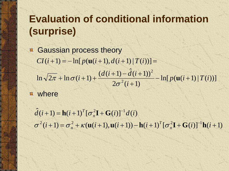
Evaluation of conditional information (surprise)

Gaussian process theory where

))](|)1((ln[)1(2

))1(ˆ)1(()1(ln2ln

))](|)1(),1((ln[)1(

2

2

iTipi

ididi

iTidipiCI

+−+

+−++++

=++−=+

u

u

σσπ

)1()]([)1())1(),1(()1(

)()]([)1()1(ˆ1222

12

+++−+++=+

++=+−

−

iiiiiiidiiid

nT

n

nT

hGIhuuGIh

σκσσ

σ

Interpretation of conditional information (surprise)

Prediction error

Large error large conditional information Prediction variance

Small error, large variance large CI Large error, small variance large CI (abnormal)

Input distribution Rare occurrence large CI

)1(ˆ)1()1( +−+=+ ididie

)1(2 +iσ

))(|)1(( iTip +u

))](|)1((ln[)1(2

))1(ˆ)1(()1(ln2ln

))](|)1(),1((ln[)1(

2

2

iTipi

ididi

iTidipiCI

+−+

+−++++

=++−=+

u

u

σσπ

Input distribution

Memoryless assumption Memoryless uniform assumption

))(|)1(( iTip +u

))1(())(|)1(( +=+ ipiTip uu

.))(|)1(( constiTiup =+

Unknown desired signal

Average CI over the posterior distribution of the output Memoryless uniform assumption This is equivalent to approximate linear dependency!

))](|)1((ln[)1(ln)1( iTipiiIC +−+=+ uσ

)1(ln)1( +=+ iiIC σ

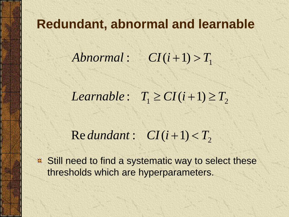
Redundant, abnormal and learnable

Still need to find a systematic way to select these thresholds which are hyperparameters.

2

21

1

)1(:Re

)1(:

)1(:

TiCIdundant

TiCITLearnable

TiCIAbnormal

<+

≥+≥

>+

Active online GP regression (AOGR)

Compute conditional information If redundant

Throw away

If abnormal Throw away (outlier examples) Controlled gradient descent (non-stationary)

If learnable Kernel recursive least squares (stationary) Extended KRLS (non-stationary)

Simulation-5: nonlinear regression—learning curve

Simulation-5: nonlinear regression—redundancy removal

T1 is wrong, should be T2

Simulation-5: nonlinear regression– most surprising data

Simulation-5: nonlinear regression

Simulation-5: nonlinear regression— abnormality detection (15 outliers)

AOGR=KRLS

Simulation-6: Mackey-Glass time series prediction

AOGR=KRLS

Simulation-7: CO2 concentration forecasting

Quantized Kernel Least Mean Square A common drawback of sparsification methods: the redundant input data are purely discarded! Actually the redundant data are very useful and can be, for example, utilized to update the coefficients of the current network, although they are not so important for structure update (adding a new center). Quantization approach: the input space is quantized, if the current quantized input has already been assigned a center, we don’t need to add a new, but update the coefficient of that center with the new information! Intuitively, the coefficient update can enhance the utilization efficiency of that center, and hence may yield better accuracy and a more compact network.

Chen B., Zhao S., Zhu P., Principe J. Quantized Kernel Least Mean Square Algorithm, submitted to IEEE Trans. Neural Networks

Quantized Kernel Least Mean Square

Quantization in Input Space

Quantization in RKHS Using the quantization method to

compress the input (or feature) space and hence to compact the RBF structure of the kernel adaptive filter

[ ]

(0)( ) ( ) ( 1) ( )( ) ( 1) ( ) ( )

Te i d i i ii i e i iη

=

= − − = − +

0Ω

Ω

Ω Ω

ϕϕQ

[ ]( )

0

1

1

0( ) ( ) ( ( ))

( ) ( ) ,i

i i

fe i d i f i

f f e i Q iη κ−

−

= = − = +

u

u .

Quantization operator


The key problem is the vector quantization (VQ): Information Theory? Information Bottleneck? …… Most of the existing VQ algorithms, however, are not suitable for online implementation because the codebook must be supplied in advance (which is usually trained on an offline data set), and the computational burden is rather heavy. A simple online VQ method:

1. Compute the distance between u(i) and C(i-1) : 2. If keep the codebook unchanged, and quantize u(i) into

the closest code-vector by 3. Otherwise, update the codebook: , and quantize u(i) as itself

( )( )1 ( 1)

( ), ( 1) min ( ) ( 1)jj size idis i i i i

≤ ≤ −− = − −u u

CC C

( )( ), ( 1)dis i i ε− ≤u UC

( ) ( 1), ( )i i i= − uC C

( )

*

1 ( 1)arg min ( ) ( 1)jj size i

j i i≤ ≤ −

= − −uC

C * *( ) ( 1) ( )j j

i i e iη= − +a a


Quantized Energy Conservation Relation

A Sufficient Condition for Mean Square Convergence Steady-state Mean Square Performance

( ) ( )222 2

2 2

( )( )( ) ( 1)( ), ( ) ( ), ( )

paq

q q

e ie ii ii i i i

βκ κ

+ = − + + Ω Ωu u u uF F

2 2

( ) ( 1) ( ) 0 ( 1)

, 2 ( ) ( 1) ( )0 ( 2)

( )

Ta q

Ta q

a v

E e i i i C

i E e i i iC

E e iη

σ

− > ∀ − < ≤ +

Ω

Ω

ϕ

ϕ

2 22max ,0 lim ( )

2 2v v

aiE e iγ γησ ξ ησ ξ

η η→∞

− + ≤ ≤ − −

2 2


Static Function Estimation

2 2( ( ) 1) ( ( ) 1)( ) 0.2 exp exp ( )2 2

u i u id i v i + −

= × − + − +

10-2 10-1 100 10110-2

10-1

quantization factor γ

EM

SE

Lower bound

Upper bound

EMSE = 0.0171

2 4 6 8 100.10

10

20

30

40

quantization factor γ

final

net

wor

k si

ze


Short Term Lorenz Time Series Prediction

0 1000 2000 3000 40000

50

100

150

200

250

300

350

400

450

500

iteration

netw

ork

size

QKLMSNC-KLMSSC-KLMS

0 1000 2000 3000 400010-3

10-2

10-1

100

101

iteration

test

ing

MS

E

QKLMSNC-KLMSSC-KLMS


Short Term Lorenz Time Series Prediction

0 1000 2000 3000 40000

50

100

150

200

250

300

350

400

iteration

netw

ork

size

QKLMSNC-KLMSSC-KLMS

0 1000 2000 3000 400010-3

10-2

10-1

100

101

iteration

test

ing

MS

E

QKLMSNC-KLMSSC-KLMSKLMS

Redefinition of On-line Kernel Learning

Notice how problem constraints affected the form of the learning algorithms.

On-line Learning: A process by which the free parameters and the topology of a ‘learning system’ are adapted through a process of stimulation by the environment in which the system is embedded.

Error-correction learning + memory-based learning What an interesting (biological plausible?) combination.

Impacts on Machine Learning

KAPA algorithms can be very useful in large scale learning problems.

Just sample randomly the data from the data base and apply on-line learning algorithms

There is an extra optimization error associated with these methods, but they can be easily fit to the machine contraints (memory, FLOPS) or the processing time constraints (best solution in x seconds).

Information Theoretic Learning (ITL)

This class of algorithms can be extended to ITL cost functions and also beyond Regression (classification, Clustering, ICA, etc). See IEEE SP MAGAZINE, Nov 2006 Or ITL resource www.cnel.ufl.edu

Kernel Adaptive Filtering - Computational … · Outline 1. Optimal adaptive signal processing...

Documents

Transcript of Kernel Adaptive Filtering - Computational … · Outline 1. Optimal adaptive signal processing...