Kent Academic Repository · , (2.1) for a suitable Hamiltonian function HJ(q,p,z) (see Okamoto...

Kent Academic RepositoryFull text document (pdf)

Copyright & reuse

Content in the Kent Academic Repository is made available for research purposes. Unless otherwise stated all

content is protected by copyright and in the absence of an open licence (eg Creative Commons), permissions

for further reuse of content should be sought from the publisher, author or other copyright holder.

Versions of research

The version in the Kent Academic Repository may differ from the final published version.

Users are advised to check http://kar.kent.ac.uk for the status of the paper. Users should always cite the

published version of record.

Enquiries

For any further enquiries regarding the licence status of this document, please contact:

[email protected]

If you believe this document infringes copyright then please contact the KAR admin team with the take-down

information provided at http://kar.kent.ac.uk/contact.html

Citation for published version

Clarkson, Peter (2008) The fourth Painleve equation. In: Guo, Li and Sit, William Y., eds.Differential Algebra and Related Topics. World Scientific, Singapore. ISBN 978-981-283-371-6.

DOI

Link to record in KAR

https://kar.kent.ac.uk/23090/

Document Version

UNSPECIFIED

The Fourth Painleve Transcendent

P. A. CLARKSON,

Institute of Mathematics, Statistics and Actuarial Science,

University of Kent, Canterbury, CT2 7NF, UK

E-mail: [email protected]

13 November 2008

Abstract

The six Painleve equations (PI–PVI) were first discovered about a hundred years ago by Painleve and his col-

leagues in an investigation of nonlinear second-order ordinary differential equations. During the past 30 years there

has been considerable interest in the Painleve equations primarily due to the fact that they arise as symmetry reductions

of the soliton equations which are solvable by inverse scattering. Although first discovered from pure mathematical

considerations, the Painleve equations have arisen in a variety of important physical applications.

The Painleve equations may be thought of as nonlinear analogues of the classical special functions. They have

a Hamiltonian structure and associated isomonodromy problems, which express the Painleve equations as the com-

patibility condition of two linear systems. The Painleve equations also admit symmetries under affine Weyl groups

which are related to the associated Backlund transformations. These can be used to generate hierarchies of rational

solutions and one-parameter families of solutions expressible in terms of the classical special functions, for special

values of the parameters. Further solutions of the Painleve equations have some interesting asymptotics which are

use in applications. In this paper I discuss some of the remarkable properties which the Painleve equations possess

using the fourth Painleve equation (PIV) as an illustrative example.

1 Introduction

The six Painleve equations (PI–PVI) are the nonlinear ordinary differential equations

w′′ = 6w2 + z, (1.1)

w′′ = 2w3 + zw + α, (1.2)

w′′ =(w′)

2

w− w′

z+αw2 + β

z+ γw3 +

δ

w, (1.3)

w′′ =(w′)

2

2w+

3

2w3 + 4zw2 + 2(z2 − α)w +

β

w, (1.4)

w′′ =

(1

2w+

1

w − 1

)(w′)

2 − w′

z+

(w − 1)2

z2

(αw +

β

w

)+γw

z+δw(w + 1)

w − 1, (1.5)

w′′ =1

2

(1

w+

1

w − 1+

1

w − z

)(w′)

2 −(

1

z+

1

z − 1+

1

w − z

)w′

+w(w − 1)(w − z)

z2(z − 1)2

{α+

βz

w2+γ(z − 1)

(w − 1)2+δz(z − 1)

(w − z)2

}, (1.6)

where ′ ≡ d/dz and α, β, γ and δ are arbitrary constants, whose solutions are called the Painleve transcendents.

The Painleve equations PI–PVI were discovered about a hundred years ago by Painleve, Gambier and their colleagues

whilst studying which second order ordinary differential equations of the form

w′′ = F (z;w,w′) , (1.7)

where F is rational in w′ and w and analytic in z, have the property that the solutions have no movable branch points,

i.e. the locations of multi-valued singularities of any of the solutions are independent of the particular solution chosen

and so are dependent only on the equation; this is now known as the Painleve property. Painleve, Gambier et al.

showed that there were fifty canonical equations of the form (1.7) with this property, up to a Mobius (bilinear rational)

transformation

W (ζ) =a(z)w + b(z)

c(z)w + d(z), ζ = φ(z), (1.8)

where a(z), b(z), c(z), d(z) and φ(z) are locally analytic functions. Further they showed that of these fifty equations,

forty-four are either integrable in terms of previously known functions (such as elliptic functions or are equivalent

to linear equations) or reducible to one of six new nonlinear ordinary differential equations, which define new tran-

scendental functions (see Ince (48)). The Painleve equations can be thought of as nonlinear analogues of the classical

special functions (see Refs. (23; 30; 52; 100)). Indeed Iwasaki, Kimura, Shimomura and Yoshida (52) characterize the

Painleve equations as “the most important nonlinear ordinary differential equations” and state that “many specialists

believe that during the twenty-first century the Painleve functions will become new members of the community of

special functions”. Further Umemura (100) states that “Kazuo Okamoto and his circle predict that in the 21st century

a new chapter on Painleve equations will be added to Whittaker and Watson’s book”.

Although first discovered from mathematical considerations, the Painleve equations have subsequently arisen in a

variety of applications including statistical mechanics (correlation functions of the XY model and the Ising model),

random matrix theory, topological field theory, plasma physics, nonlinear waves (resonant oscillations in shallow wa-

ter, convective flows with viscous dissipation, Gortler vortices in boundary layers and Hele-shaw problems), quantum

gravity, quantum field theory, general relativity, nonlinear and fiber optics, polyelectrolytes, Bose-Einstein conden-

sation and stimulated Raman scattering. Further the Painleve equations have attracted much interest since they also

arise as reductions of the soliton equations, such as the Korteweg-de Vries, Boussinesq and nonlinear Schrodinger

equations, which are solvable by inverse scattering (see Ablowitz and Clarkson (2) and references therein).

The general solutions of the Painleve equations are transcendental, i.e. irreducible in the sense that they cannot be

expressed in terms of previously known functions, such as rational functions, elliptic functions or the classical special

functions (see Umemura (100)). Essentially, generic solutions of the PI–PV are meromorphic functions in the complex

plane (see Hinkkanen and Laine (44–46) and Steinmetz (93), also Gromak, Laine and Shimomura (42)); solutions of

PVI are rather different since the equation has three singular points (see Hinkkanen and Laine (47)).

The Painleve equations, in common with other integrable equations such as soliton equations, have a plethora of

fascinating properties, some of which we discuss in the following sections, using PIV (1.4) as an illustrative example.

• The equations PI–PVI can be written as a (non-autonomous) Hamiltonian system, which are discussed in equa-

tion (2.

• The equations PI–PVI can be expressed as the compatibility condition of a linear system, called an isomon-

odromy problem or Lax pair, which are discussed in §3.

• The equations PII–PVI possess Backlund transformations which relate one solution to another solution either of

the same equation, with different values of the parameters, or another equation, which are discussed in §4; these

transformations play an important role in the theory of integrable systems.

• The equations PII–PVI possess many rational solutions, algebraic solutions and solutions expressible in terms

of the classical special functions for certain values of the parameters, which are discussed in Secs. 5–6; these

solutions of the Painleve equations are called “classical solutions”, see Umemura(100).

• Since the solutions of the equations PI–PVI are transcendental, then a study of the asymptotic behaviour of

these solutions, together with the associated connection formulae which relate the asymptotic behaviours of the

solutions as z → ±∞, play an important role in the application of the equations. These are discussed in §7.

A representation of PIV which has attracted much recent interest is the symmetric PIV (sPIV) system

ϕ′

1 + ϕ1(ϕ2 − ϕ3) + 2µ1 = 0, (1.9a)

ϕ′

2 + ϕ2(ϕ3 − ϕ1) + 2µ2 = 0, (1.9b)

ϕ′

3 + ϕ3(ϕ1 − ϕ2) + 2µ3 = 0, (1.9c)

where µ1, µ2 and µ3 are constants, with the constraints

µ1 + µ2 + µ3 = 1, ϕ1 + ϕ2 + ϕ3 = −2z. (1.9d)

Eliminating ϕ2 and ϕ3, then w = ϕ1 satisfies PIV (1.4) with α = µ3 − µ2 and β = −2µ21. The system sPIV (1.9)

was derived by Bureau (15; 16) and later by Adler (5). The sPIV system (1.9) is extensively discussed by Noumi (79)

and arises in applications such as random matrices (see Forrester and Witte (35; 36)); other studies of sPIV include

Refs. (55; 72; 80; 83; 90–92; 94; 99; 106; 109).

2

2 Hamiltonian Structure

The Hamiltonian structure associated with the Painleve equations PI–PVI is HJ = (q, p,HJ, z), where HJ, the Hamil-

tonian function, is a polynomial in q, p and rational in z. Each of the Painleve equations PI–PVI can be written as a

Hamiltonian systemdq

dz=∂HJ

∂p,

dp

dz= −∂HJ

∂q, (2.1)

for a suitable Hamiltonian function HJ(q, p, z) (see Okamoto (88)). Further the function σ(z) ≡ HJ(q, p, z) satisfies

a second-order, second-degree ordinary differential equation, whose solution is expressible in terms of the solution of

the associated Painleve equation.

Example 2.1. The Hamiltonian for PIV (1.4) is

HIV(q, p, z) = 2qp2 − (q2 + 2zq + 2κ0)p+ κ∞q, (2.2)

with κ0 and κ∞ parameters, and so

q′ = 4qp− q2 − 2zq − 2κ0, (2.3a)

p′ = −2p2 + 2pq + 2zp− κ∞. (2.3b)

Eliminating p then w = q satisfies PIV (1.4) with α = 1 − κ0 + 2κ∞ and β = −2κ20, whilst eliminating q then

w = −2p satisfies PIV (1.4) with α = 2κ0 −κ∞−1 and β = −2κ2∞. The function σ = HIV(q, p, z), defined by (2.2)

satisfies the second-order second-degree ordinary differential equation

(σ′′)2 − 4 (zσ′ − σ)

2+ 4σ′ (σ′ + 2κ0) (σ′ + 2κ∞) = 0 (2.4)

(see Jimbo and Miwa (53) and Okamoto (84)). Equation (2.4) is equivalent to equation SD-I.c in the classification of

second order, second degree ordinary differential equations with the Painleve property due to Cosgrove and Scoufis

(27), an equation first derived and solved by Chazy (17) and rederived by Bureau (13; 14). Equation (2.4 also arises

in various applications including random matrix theory, see, for example, Refs. (35; 36; 57; 98). Conversely, if σ is a

solution of (2.4), then solutions of (2.3) are given by

q =σ′′ − 2zσ′ + 2σ

2(σ′ + 2κ∞), p =

σ′′ + 2zσ′ − 2σ

4(σ′ + 2κ0). (2.5)

We remark for sPIV (1.9), the Hamiltonian is

HIV(ϕ1, ϕ2, ϕ3, z) = − 12ϕ1ϕ2ϕ3 + µ1ϕ2 − µ2ϕ1, (2.6)

since q = ϕ1, p = − 12ϕ2, κ0 = µ1 and κ∞ = −µ2.

3 Isomonodromy Problems

Each of the Painleve equations PI–PVI can be expressed as the compatibility condition of the linear system

∂Ψ

∂λ= A(z;λ)Ψ,

∂Ψ

∂z= B(z;λ)Ψ, (3.1)

where A and B are matrices whose entries depend on the solution w(z) of the Painleve equation. The equation

∂2Ψ

∂z∂λ=

∂2Ψ

∂λ∂z,

is satisfied provided that∂A

∂z− ∂B

∂λ+ AB − BA = 0, (3.2)

which is the compatibility condition of (3.1). Matrices A and B for PI–PVI satisfying (3.2) are given by Jimbo and

Miwa (54) (see also Refs. (30) and (51)), though these are not unique, as illustrated in the following exmaples.

3

Example 3.1. Jimbo and Miwa (54) show that the compatibility condition of the linear system (3.1) with

A(z;λ) =

λ+ z +θ0 − 2v

2λu− uw

2λ2v − θ0 − θ∞

u+

2v(v − θ0)

λuw−λ− z +

2v − θ02λ

, (3.3a)

B(z;λ) =

(λ u

2v − θ0 − θ∞u

λ

), (3.3b)

with θ0 and θ∞ parameters, is

u′ = −u(w + 2z), (3.4a)

v′ =2θ0 − 2v2

w+ 1

2 (θ0 + θ∞ − 2v)w, (3.4b)

w′ = −4v + w2 + 2zw + 2θ0. (3.4c)

Eliminating v then w satisfies PIV (1.4) with α = θ∞ − 1 and β = −2θ20 .

Example 3.2. As remarked above, the isomonodromy problem is not unique. Kitaev (60) and Milne, Clarkson and

Bassom (74) show that PIV (1.4) also arises as the compatibility condition of the linear system (3.1) with

A(z;λ) =

12λ

3 + (z + uv) +Θ0

λi(λ2 + 2zu+ u′)

i(λ2 + 2zv − v′) − 12λ

3 − (z + uv) − Θ0

λ

, (3.5a)

B(z;λ) =

(12λ

2 + uv iλuiλv − 1

2λ2 − uv

). (3.5b)

with Θ0 a constant, which comes from a scaling reduction of the Lax pair for the modified nonlinear Schrodinger

equation

iut = uxx + i(|u|2u)x, (3.6)

due to Kaup and Newell (59). Substituting (3.5) into the compatibility condition (3.2) yields

u′′ + 2zu′ + u+ 2Θ0u− 4zu2v − 2uvu′ = 0, (3.7a)

v′′ − 2zv′ − v + 2Θ0v − 4zuv2 + 2uvv′ = 0, (3.7b)

which implies that

u′v − uv′ + 2zuv − u2v2 = 2Θ1, (3.8)

with Θ1 a constant. Then w = uv satisfies PIV (1.4) with α = 2Θ0 − Θ1 and β = −2Θ21.

4 Backlund and Schlesinger Transformations

4.1 Backlund Transformations

The Painleve equations PII–PVI possess Backlund transformations which relate one solution to another solution either

of the same equation, with different values of the parameters, or another equation (see Refs. (23; 28; 42) and the

references therein). An important application of the Backlund transformations is that they generate hierarchies of

classical solutions of the Painleve equations, which are discussed in §5 and §6.

Theorem 4.1. Let w0 = w(z;α0, β0) and w±

j = w(z;α±

j , β±

j ), j = 1, 2, 3, 4 be solutions of PIV (1.4) with

α±

1 = 14 (2 − 2α0 ± 3

√−2β0), β±

1 = − 12 (1 + α0 ± 1

2

√−2β0)

2, (4.1a)

α±

2 = − 14 (2 + 2α0 ± 3

√−2β0), β±

2 = − 12 (1 − α0 ± 1

2

√−2β0)

2, (4.1b)

α±

3 = 32 − 1

2α0 ∓ 34

√−2β0, β±

3 = − 12 (1 − α0 ± 1

2

√−2β0)

2, (4.1c)

α±

4 = − 32 − 1

2α0 ∓ 34

√−2β0, β±

4 = − 12 (−1 − α0 ± 1

2

√−2β0)

2. (4.1d)

4

Table 4.1: The effect of the Backlund transformations of sPIV

µ1 µ2 µ3 ϕ1 ϕ2 ϕ3

S1 −µ1 µ1 + µ2 µ1 + µ3 ϕ1 ϕ2 −2µ1

ϕ1ϕ3 −

2µ1

ϕ1

S2 µ1 + µ2 −µ2 µ2 + µ3 ϕ1 −2µ2

ϕ2ϕ2 ϕ3 +

2µ2

ϕ2

S3 µ1 + µ3 µ2 + µ3 −µ3 ϕ1 +2µ3

ϕ3ϕ2 −

2µ3

ϕ3ϕ3

π µ2 µ3 µ1 ϕ2 ϕ3 ϕ1

Then

T ±

1 : w±

1 =w′

0 − w20 − 2zw0 ∓

√−2β0

2w0, (4.2a)

T ±

2 : w±

2 = − w′0 + w2

0 + 2zw0 ∓√−2β0

2w0, (4.2b)

T ±

3 : w±

3 = w0 +2(1 − α0 ∓ 1

2

√−2β0

)w0

w′0 ±

√−2β0 + 2zw0 + w2

0

, (4.2c)

T ±

4 : w±

4 = w0 +2(1 + α0 ± 1

2

√−2β0

)w0

w′0 ∓

√−2β0 − 2zw0 − w2

0

, (4.2d)

valid when the denominators are non-zero, and where the upper signs or the lower signs are taken throughout each

transformation.

Proof. See Lukashevich (64), Gromak (40; 41); also Bassom, Clarkson and Hicks (8), Gromak, Laine and Shimomura

(42) and Murata (77).

The parameter space of PIV can be identified with the Cartan subalgebra of a simple Lie algebra and the corre-

sponding affine Weyl group A2 acts on PIV as a group of Backlund transformations (for further details see Refs. (80;

83; 84; 101)). An affine Weyl group is essentially a group of translations and reflections on a lattice, which for PIV is

in the parameter space. The affine Weyl group A2 = 〈S0,S1,S2,π〉 with fundamental relations

S2j = I, (SjSj+1)

3 = I, π3 = I, πSj = Sj+1π, (4.3)

for j = 1, 2, 3, with Sj+3 = Sj for j ∈ Z.

Theorem 4.2. The Backlund transformations of sPIV (1.9) are defined by the fundamental relations (4.3) and realized

as a group of automorphisms of the field of rational functions C(µj , ϕj), for j = 1, 2, 3, as

Sj(µj) = −µj , Sj(µj±1) = µj±1 + µj , (4.4a)

Sj(ϕj) = ϕj , Sj(ϕj±1) = ϕj±1 ±µj

ϕj, (4.4b)

π(µj) = µj+1, π(ϕj) = ϕj+1. (4.4c)

Proof. See Noumi and Yamada (80; 82); see also Noumi (79). The effect of these Backlund transformations is

summarized in Table 4.1.

Discrete Painleve equations, which are discrete equations (difference equations) that have Painleve equations as

their continuum limits, arising from the Backlund transformations of PIV (1.4) given by (4.2) are discussed in Refs. (26;

29; 38), as illustrated in the following example.

Example 4.3. Consider the Backlund transformations T +1 and T −

2 . Setting an+1 = α+1 , an = α0, an−1 = α−

2 ,

cn+1 =√

−2(β+1 )2, cn =

√−2β2

0 and cn−1 =√

−2(β−

2 )2 yields the difference equations

an+1 = 12 − 1

2an + 34cn, an−1 = − 1

2 + 12an − 3

4cn,

cn+1 = 1 + an + 12cn, cn−1 = −1 + an + 1

2cn,

5

which have the solution

an = 12κ− 3

2µ(−1)n

+ 12n, cn = κ+ µ(−1)

n+ n,

with κ and µ arbitrary constants. Eliminating w′0 between the Backlund transformations T +

1 and T −

2 , then setting

xn = w0(z; an, cn), xn+1 = w+1 (z; an+1, cn+1) and xn−1 = w−

2 (z; an−1, cn−1), with cm =√−2bm, gives

(xn+1 + xn + xn−1)xn = −2zxn − n+ κ(−1)n + µ, (4.5)

which is the discrete Painleve equation dPI (29). The relationship between solutions of PIV (1.4) and solutions of

dPI (4.5) was first noted by Fokas, Its and Kapaev (31; 32). Subsequently this relationship was studied by Bassom,

Clarkson and Hicks (8) who derived hierarchies of simultaneous solutions of PIV (1.4) and dPI (4.5) in terms of

parabolic cylinder functions (the half-integer hierarchy discussed in §6.3); see also Ref. (38). The relationship between

solutions of PIV (1.4) and dPI (4.5) is reflected in the similarity of the results for dPI in Ref. (38) to those for PIV in

Refs. (8; 77; 84; 103).

4.2 Schlesinger transformations

A class of Backlund transformations for the Painleve equations is generated by so-called Schlesinger transformations

of the associated isomondromy problems (see Refs. (33) and (76)).

Fokas, Mugan and Ablowitz (33), using a Schlesinger transformation formulation associated with the isomon-

odromy formulation of PIV, deduced the following transformations R1–R4 for PIV.

R1 : w1 =

(w′ +

√−2β

)2+(4α+ 4 − 2

√−2β

)w2 − w2(w + 2z)2

2w(w2 + 2zw − w′ −

√−2β

) , (4.6a)

R2 : w2 =

(w′ −

√−2β

)2+(4α− 4 − 2

√−2β

)w2 − w2(w + 2z)2

2w(w2 + 2zw + w′ −

√−2β

) , (4.6b)

R3 : w3 =

(w′ −

√−2β

)2 −(4α+ 4 + 2

√−2β

)w2 − w2(w + 2z)2

2w(w2 + 2zw − w′ +

√−2β

) , (4.6c)

R4 : w4 =

(w′ +

√−2β

)2+(4α− 4 + 2

√−2β

)w2 − w2(w + 2z)2

2w(w2 + 2zw + w′ +

√−2β

) , (4.6d)

where w ≡ w(z;α, β), wj ≡ w(z;αj , βj). Fokas, Mugan and Ablowitz (33) also defined the composite transforma-

tions R5 = R1R3, R+6 ≡ R2R3, R−

6 ≡ R1R4 and R7 = R2R4 given by

R5 : w5 =

(w′ − w2 − 2zw

)2+ 2β

2w {w′ − w2 − 2zw + 2 (α+ 1)} , (4.7a)

R±

6 : w6 = w +

(2α− 2 ∓

√−2β

)wM±(w,w′, z)

w(4 ± 2√−2β) −M±(w,w′, z)

(w′ − 2zw − w2 ∓

√−2β

)

+

(2 + 2α±

√−2β

)w

w′ − 2zw − w2 ∓√−2β

+2 ±

√−2β

M±(w,w′, z), (4.7b)

R7 : w7 =

(w′ + w2 + 2zw

)2+ 2β

2w {w′ + w2 + 2zw − 2 (α− 1)} , (4.7c)

respectively, where

M±(w,w′, z) = 12w + z +

(2 + 2α±

√−2β

)w

w′ − 2zw − w2 ∓√−2β

+w′ ∓

√−2β

2w. (4.7d)

We remark that R5 and R7 are the transformations T+ and T−, respectively, given by Murata (77) and a special case

of R±

6 is given by Boiti and Pempinelli (11). Further note that w1 and w2 in (4.6a,b) are respectively xn±2 in the

sense of (4.5). The effect of these Schlesinger transformations on the PIV parameters α and β, the isomonodromy

parameters θ0 and θ∞, and the sPIV parameters µ1, µ2 and µ3 is given in Table 4.2.

The Schlesinger transformations R1–R5, R±

6 and R7 are Backlund transformations of PIV which involve (w′)2.

The Backlund transformations for PIV given by T ±

1 –T ±

4 (4.2), have the form

w(z; α, β) =A(w, z)w′ +B(w, z)

C(w, z)w′ +D(w, z), (4.8)

6

Table 4.2: The effect of the Schlesinger transformations R1–R5, R±

6 and R7 on the parameters.

α β θ0 θ∞ µ1 µ2 µ3

R1 α+ 1 − 12

(2 −

√−2β

)2θ0 − 1 θ∞ + 1 µ1 − 1 µ2 µ3 + 1

R2 α− 1 − 12

(2 +

√−2β

)2θ0 + 1 θ∞ − 1 µ1 + 1 µ2 µ3 − 1

R3 α+ 1 − 12

(2 +

√−2β

)2θ0 + 1 θ∞ + 1 µ1 + 1 µ2 − 1 µ3

R4 α− 1 − 12

(2 −

√−2β

)2θ0 − 1 θ∞ − 1 µ1 − 1 µ2 + 1 µ3

R5 ≡ R1R3 α+ 2 β θ0 θ∞ + 2 µ1 µ2 − 1 µ3 + 1

R+6 ≡ R2R3 α − 1

2

(4 +

√−2β

)2θ0 + 2 θ∞ µ1 + 2 µ2 − 1 µ3 − 1

R−

6 ≡ R1R4 α − 12

(4 −

√−2β

)2θ0 − 2 θ∞ µ1 − 2 µ2 + 1 µ3 + 1

R7 ≡ R2R4 α− 2 β θ0 θ∞ − 2 µ1 µ2 + 1 µ3 − 1

where A(w, z), B(w, z), C(w, z) and D(w, z) are polynomials in w and locally analytic in z, with AD − BC 6= 0;

for further details see Refs. (41) and (64). Bassom, Clarkson and Hicks (8) show that the Schlesinger transformations

R1–R5, R±

6 and R7 can be written in terms of the Backlund transformations T ±

1 –T ±

4 (4.2). Second order difference

equations which are linear the highest coefficient, in particular the discrete Painleve equations, can be derived from

Backlund transformations of the form (4.8), cf. Ref. (29), whereas Backlund transformations which involve (w′)2

usually give rise to difference equations that are of second degree in the highest coefficient, cf. Ref. (26).

5 Rational solutions of PIV

The Painleve equations PII–PVI possess sets of rational solutions, often called hierarchies, for special values of the

parameters (see Refs. (4; 23; 42) and the references therein). These hierarchies can be generated from “seed solutions”,

such as the simple solution for PIV (1.4) given in (5.1) using the Backlund transformations discussed in §4 above and

frequently are expressed in the form of determinants.

Simple rational solutions of PIV (1.4) are

w1(z;±2,−2) = ±1/z, w2(z; 0,−2) = −2z, w3(z; 0,− 29 ) = − 2

3z. (5.1)

It is known that there are three sets of rational solutions of PIV, which have the solutions (5.1) as the simplest members.

These sets are known as the “−1/z hierarchy”, the “−2z hierarchy” and the “− 23z hierarchy”, respectively (see

Bassom, Clarkson and Hicks (8)). The “−1/z hierarchy” and the “−2z hierarchy” form the set of rational solutions

of PIV (1.4) with parameters given by (5.2) and the “− 23z hierarchy” forms the set with parameters given by (5.3).

The rational solutions of PIV (1.4) with parameters given by (5.2) lie at the vertexes of the “Weyl chambers” and those

with parameters given by (5.3) lie at the centres of the “Weyl chamber”, see Umemura and Watanabe (103). The

corresponding simple rational solutions of sPIV (1.9) are

ϕ1 = −1/z, ϕ2 = 1/z, ϕ3 = −2z,

with parameters µ1 = µ2 = 1 and µ3 = −1 and

ϕ1 = ϕ2 = ϕ3 = − 23z,

with parameters µ1 = µ2 = µ3 = 13 .

Theorem 5.1. PIV (1.4) has rational solutions if and only if the parameters α and β are given by either

α = m, β = −2(2n−m+ 1)2, (5.2)

or

α = m, β = −2(2n−m+ 13 )2, (5.3)

with m,n ∈ Z. Further the rational solutions for these parameters are unique.

7

Proof. See Lukashevich (64), Gromak (41) and Murata (77); also Bassom, Clarkson and Hicks (8), Gromak, Laine

and Shimomura (42), Umemura and Watanabe (103).

In a comprehensive study of properties of solutions of PIV, Okamoto (84) introduced two sets of polynomials

associated with rational solutions of PIV, analogous to the Yablonskii–Vorob’ev polynomials, which are special poly-

nomials associated with rational solutions of PII (for further details see Refs. (25; 107; 110)). Noumi and Yamada

(83) generalized Okamoto’s results and introduced the generalized Hermite polynomials Hm,n, defined in Theorem

5.2, and the generalized Okamoto polynomials Qm,n, defined in Theorem 5.4 (see also Clarkson (20)). Noumi and

Yamada (83) expressed the generalized Hermite and generalized Okamoto polynomials in terms of Schur functions

related to the modified Kadomtsev-Petviashvili hierarchy. Kajiwara and Ohta (56) also expressed rational solutions of

PIV in terms of Schur functions by expressing the solutions in the form of determinants, see equation (5.8.

5.1 Generalized Hermite polynomials

Here we consider the generalized Hermite polynomials Hm,n which are defined in the following theorem.

Theorem 5.2. Suppose Hm,n satisfies the recurrence relations

2mHm+1,nHm−1,n = Hm,nH′′

m,n −(H ′

m,n

)2+ 2mH2

m,n, (5.4a)

2nHm,n+1Hm,n−1 = −Hm,nH′′

m,n +(H ′

m,n

)2+ 2nH2

m,n, (5.4b)

with H0,0 = H1,0 = H0,1 = 1 and H1,1 = 2z, then solutions of PIV are

w[1]m,n = w(z; 2m+ n+ 1,−2n2) =

d

dzln

(Hm+1,n

Hm,n

), (5.5a)

w[2]m,n = w(z;−(m+ 2n+ 1),−2m2) =

d

dzln

(Hm,n

Hm,n+1

), (5.5b)

w[3]m,n = w(z;n−m,−2(m+ n+ 1)2) = −2z +

d

dzln

(Hm,n+1

Hm+1,n

). (5.5c)

Proof. See Theorem 4.4 in Noumi and Yamada (83); also Theorem 3.1 in Clarkson (20). In terms of the rational

solutions (5.5), the corresponding rational solutions of sPIV (1.9) are given by ϕj = w[j]m,n, for j = 1, 2, 3, with

parameters µ1 = −n, µ2 = −m and µ3 = m+ n+ 1.

The polynomials Hm,n defined by (5.4) are called the generalized Hermite polynomials since Hm,1(z) = Hm(z)and H1,m(z) = i−mHm(iz), where Hm(z) is the standard Hermite polynomial defined by

Hm(z) = (−1)m exp(z2)dm

dzm

{exp(−z2)

}(5.6)

or alternatively through the generating function

∞∑

m=0

Hm(z)λm

m!= exp(2λz − λ2) (5.7)

(cf. Refs. (3; 6; 97)). The rational solutions of PIV defined by (5.5) include all solutions in the “−1/z” and “−2z”

hierarchies, i.e. the set of rational solutions of PIV with parameters given by (5.2), and can be expressed in terms of

determinants whose entries are Hermite polynomials; see equation (5.8. These rational solutions of PIV are special

cases of the special function solutions which are expressible in terms of parabolic cylinder functions Dν(ξ), as shown

in §6.2. The polynomial Hm,n has degree mn with integer coefficients, in fact Hm,n( 12ζ) is a monic polynomial in

ζ with integer coefficients (for further details see Refs. (20; 83)). Further Hm,n possesses the symmetry Hn,m(z) =i−mnHm,n(iz).

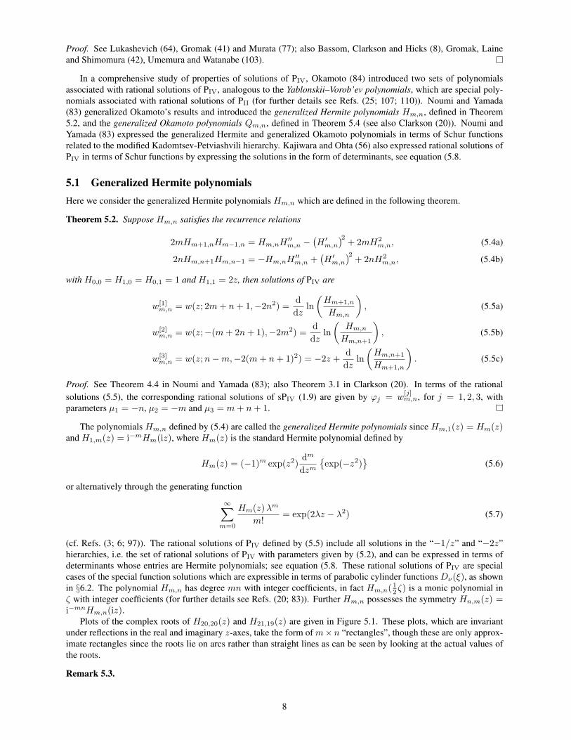
Plots of the complex roots of H20,20(z) and H21,19(z) are given in Figure 5.1. These plots, which are invariant

under reflections in the real and imaginary z-axes, take the form of m×n “rectangles”, though these are only approx-

imate rectangles since the roots lie on arcs rather than straight lines as can be seen by looking at the actual values of

the roots.

Remark 5.3.

8

–10

–5

0

5

10

–10 –5 0 5 10

–10

–5

0

5

10

–10 –5 0 5 10

H20,20(z) H21,19(z)

Figure 5.1: Roots of the generalized Hermite polynomials H20,20(z), H21,19(z)

1. The generalized Hermite polynomials Hm,n can be expressed in determinantal form as follows

Hm,n(z) = cm,nW(Hm, Hm+1, . . . ,Hm+n−1), (5.8)

where Hn(z) is the nth Hermite polynomial, cm,n is a constant and W(ϕ1, ϕ2, . . . , ϕn) is the usual Wronskian.

The generalized Hermite polynomials Hm,n can also be expressed in terms of Schur polynomials; for further

details see Kajiwara and Ohta (56) and Noumi and Yamada(83).

2. Using the Hamiltonian formalism for PIV discussed in §2, it can be shown that the generalized Hermite poly-

nomials Hm,n, which are defined by the differential-difference equations (5.4), also satisfy fourth order bilinear

ordinary differential equation

Hm,nH′′′′

m,n − 4H ′

m,nH′′′

m,n + 3(H ′′

m,n

)2+ 4zHm,nH

′

m,n − 8mnH2m,n

− 4(z2 + 2n− 2m){Hm,nH

′′

m,n −(H ′

m,n

)2}= 0, (5.9)

and homogeneous difference equations; for further details see Clarkson(21; 22).

3. The polynomial Hm,n(z) can be expressed as the multiple integral

Hm,n(z) =πm/2

∏mk=1 k!

2m(m+2n−1)/2

∫ ∞

−∞

· · ·n

∫ ∞

−∞

n∏

i=1

n∏

j=i+1

(xi − xj)2

×n∏

k=1

(z − xk)m exp(−x2

k

)dx1 dx2 . . .dxn, (5.10)

which arises in random matrix theory; for further details see Brezin and Hikami (12), Forrester and Witte (35).

4. The orthogonal polynomials on the real line with respect to the weightw(x; z,m) = (x−z)m exp(−x2), satisfy

the three-term recurrence relation

xpn(x) = pn+1(x) + an(z;m)pn(x) + bn(z;m)pn−1(x), (5.11a)

where

an(z;m) = −1

2

d

dzlnHn+1,m

Hn,m, bn(z;m) =

nHn+1,mHn−1,m

2H2n,m

, (5.11b)

for further details see Chen and Feigin (18).

9

5.2 Generalized Okamoto polynomials

Here we consider the generalized Okamoto polynomials Qm,n which were introduced by Noumi and Yamada (83)

and are defined in following Theorem.

Theorem 5.4. Suppose Qm,n satisfies the recurrence relations

Qm+1,nQm−1,n = 92

{Qm,nQ

′′

m,n −(Q′

m,n

)2}+{2z2 + 3(2m+ n− 1)

}Q2

m,n, (5.12a)

Qm,n+1Qm,n−1 = 92

{Qm,nQ

′′

m,n −(Q′

m,n

)2}+{2z2 + 3(1 −m− 2n)

}Q2

m,n, (5.12b)

with Q0,0 = Q1,0 = Q0,1 = 1 and Q1,1 =√

2 z, then solutions of PIV are

w[1]m,n = w(z; 2m+ n,−2(n− 1

3 )2) = − 23z +

d

dzln

(Qm+1,n

Qm,n

), (5.13a)

w[2]m,n = w(z;−m− 2n,−2(m− 1

3 )2) = − 23z +

d

dzln

(Qm,n

Qm,n+1

), (5.13b)

w[3]m,n = w(z;n−m,−2(m+ n+ 1

3 )2) = − 23z +

d

dzln

(Qm,n+1

Qm+1,n

). (5.13c)

Proof. See Theorem 4.3 in Noumi and Yamada (83); also Theorem 4.1 in Clarkson (20). In terms of the rational

solutions (5.13), the corresponding rational solutions of sPIV (1.9) are given by ϕj = w[j]m,n, for j = 1, 2, 3, with

parameters µ1 = −n+ 13 , µ2 = −m+ 1

3 and µ3 = m+ n+ 13 .

The polynomials Qm,n defined by (5.12) are called the generalized Okamoto polynomials since Okamoto (84)

defined the polynomials in the cases when n = 0 and n = 1. The rational solutions of PIV defined by (5.13)

include all solutions in the “− 23z” hierarchy, i.e. the set of rational solutions of PIV with parameters given by (5.3),

which also can be expressed in the form of determinants; see equation (5.15. The polynomial Qm,n has degree

dm,n = m2 + n2 +mn−m− n with integer coefficients (83); in fact Qm,n( 12

√2 ζ) is a monic polynomial in ζ with

integer coefficients. Further Qm,n possesses the symmetries

Qn,m(z) = exp(− 12πidm,n)Qm,n(iz), (5.14a)

Q1−m−n,n(z) = exp(− 12πidm,n)Qm,n(iz). (5.14b)

Note that dm,n = m2 + n2 +mn−m− n satisfies dm,n = dn,m = d1−m−n,n.

Plots of the complex roots ofQ10,10(z) andQ−9,−7(z) are given in Figure 5.2. The roots of the polynomialQm,n,

with m,n ≥ 1, take the form of m × n “rectangle” with an “equilateral triangle”, which have either m − 1 or n − 1roots, on each of its sides. The roots of the polynomial Q−m,−n, with m,n ≥ 1, take the form of m × n “rectangle”

with an “equilateral triangle”, which now have either m or n roots, on each of its sides. These are only approximate

rectangles and equilateral triangles as can be seen by looking at the actual values of the roots. The plots are invariant

under reflections in the real and imaginary z-axes.

Due to the symmetries (5.14), the roots of the polynomials Q−m,n and Qm,−n, with m,n ≥ 1 take similar forms

as these polynomials they can be expressed in terms of QM,N and Q−M,−N for suitable M,N ≥ 1. Specifically, the

roots of the polynomial Q−m,n, with m ≥ n ≥ 1, has the form of a n× (m− n+ 1) “rectangle” with an “equilateral

triangle”, which have either n − 1 or n −m − 1 roots, on each of its sides. Also the roots of the polynomial Q−m,n

with n > m ≥ 1, has the form of a m× (n−m− 1) “rectangle” with an “equilateral triangle”, which have either mor n−m− 1 roots, on each of its sides. Further, we note that Q−m,m = Qm,1 and Q1−m,m = Qm,0, for all m ∈ Z,

where Qm,0 and Qm,0 are the original polynomials introduced by Okamoto (84). Analogous results hold for Qm,−n,

with m,n ≥ 1.

Remark 5.5.

1. The generalized Okamoto polynomials Qm,n can be expressed in determinantal form as follows

Qm,n = cm,nW (ψ1, ψ4, . . . , ψ3m+3n−5, ψ2, ψ5, . . . , ψ3n−4) , (5.15a)

Q−m,−n = cm,nW (ψ1, ψ4, . . . , ψ3n−2, ψ2, ψ5, . . . , ψ3m+3n−1) , (5.15b)

for m,n ≥ 0, with cm,n and cm,n constants, W(ψ1, ψ2, . . . , ψn) the Wronskian, and ψn(z) given by

∞∑

n=0

ψn(z) ζn

n!= exp

(2zζ + 3ζ2

), (5.16)

10

–8

–6

–4

–2

0

2

4

6

8

–6 –4 –2 0 2 4 6 8

–6

–4

–2

0

2

4

6

–6 –4 –2 0 2 4 6

Q10,10(z) Q−9,−7(z)

Figure 5.2: Roots of the generalized Okamoto polynomials Q10,10(z) and Q−9,−7(z)

so ψn(z) = (−3)n/2Hn

(13

√3 iz). This follows from equation (20) in Kajiwara and Ohta (56), though it is not

given there explicitly (see also Ref. (24)). The generalized Okamoto polynomials Qm,n can also be expressed

in terms of Schur polynomials (for further details see Refs. (24; 56; 83)).

2. As for the generalized Hermite polynomials,using the Hamiltonian formalism for PIV discussed in §2, it can

be shown that the generalized Okamoto polynomials Qm,n, which are defined by the differential-difference

equations (5.12), also satisfy the fourth order bilinear ordinary differential equation

Qm,nQ′′′

m,n − 4Q′

m,nQ′′′

m,n + 3(Q′′

m,n

)2+ 4

3z2{Qm,nQ

′′

m,n −(Q′

m,n

)2}

+ 4zQm,nQ′

m,n − 83 (m2 + n2 +mn−m− n)Q2

m,n = 0, (5.17)

and homogeneous difference equations; for details see Refs. (21) and (22).

6 Special Function Solutions

The Painleve equations PII–PVI possess hierarchies of solutions expressible in terms of classical special functions, for

special values of the parameters through an associated Riccati equation,

w′ = p2(z)w2 + p1(z)w + p0(z), (6.1)

where p2(z), p1(z) and p0(z) are rational functions. Hierarchies of solutions, which are often referred to as “one-

parameter solutions” (since they have one arbitrary constant), are generated from “seed solutions” derived from the

Riccati equation using the Backlund transformations given in §4. Furthermore, as for the rational solutions, these

special function solutions are often expressed in the form of determinants. See Sachdev (89) for details of the derivation

of the associated Riccati equations for PII–PVI.

Special function solutions of PII are expressed in terms of Airy functions Ai(z) and Bi(z)(4; 37; 40; 84), of PIII

are expressed in terms of Bessel functions Jν(z) and Yν(z) (65; 75; 78; 87; 104), of PIV in terms of Weber-Hermite

(parabolic cylinder) functions Dν(z) (8; 41; 64; 77; 84; 103), of PV in terms of Whittaker functions Mκ,µ(z) and

Wκ,µ(z), or equivalently confluent hypergeometric functions 1F1(a; c; z) (39; 66; 86; 108) and of PVI in terms of

hypergeometric functions F (a, b; c; z) (34; 68; 85); see also Refs. (23; 42; 70; 95). Some classical orthogonal poly-

nomials arise as particular cases of these special function solutions and thus yield rational solutions of the associated

Painleve equations. For PIII and PV these are in terms of associated Laguerre polynomials L(m)k (z) (71; 81), for PIV in

11

terms of Hermite polynomialsHn(z) (8; 56; 77; 84) and for for PVI in terms of Jacobi polynomials P(α,β)n (z) (69; 96).

In fact all rational solutions of PVI arise as particular cases of the special solutions given in terms of hypergeometric

functions (73).

6.1 Weber-Hermite function solutions of PIV

Theorem 6.1. PIV (1.4) has solutions expressible in terms of parabolic cylinder functions if and only if either

β = −2(2n+ 1 + εα)2, (6.2)

or

β = −2n2, (6.3)

with n ∈ Z and ε = ±1.

Proof. See Gambier (37), Gromak (41), Gromak and Lukashevich (43), Lukashevich (63; 64); also Gromak, Laine

and Shimomura (42).

In the case when n = 0 in (6.2), then the associated Riccati equation is

w′ = ε(w2 + 2zw) + 2ν, ε2 = 1, (6.4)

with PIV parameters α = −ε(1 + ν) and β = −2ν2. Letting w(z) = −εψ′ν(z; ε)/ψν(z; ε) in this equation yields the

Weber-Hermite equation

ψ′′

ν − 2εzψ′

ν + 2ενψν = 0, (6.5)

which, provided that ν 6∈ Z, has general solution

ψν(z; ε) ={C1Dν(

√2ε z) + C2Dν(−

√2ε z)

}exp

(12εz

2), (6.6)

where C1 and C2 are arbitrary constants and Dν(ζ) is the parabolic cylinder function which satisfies

d2Dν

dζ2 = (14ζ

2 − ν − 12 )Dν , (6.7)

with boundary condition

Dν(ζ) ∼ ζν exp(− 1

4ζ2), as ζ → +∞. (6.8)

Equivalently

ψν(z; ε) ={C1M 1

2ν+ 1

4, 1

4

(εz2) + C2W 1

2ν+ 1

4, 1

4

(εz2)} exp

(12εz

2)

z1/2, (6.9)

where C1 and C2 are arbitrary constants, and Mκ,µ(ξ) and Wκ,µ(ξ) are the Whittaker functions which satisfy

d2u

dξ2+

( 14 − µ2

ξ2+κ

ξ− 1

4

)u = 0. (6.10)

The seed solutions which generate the special function solutions of PIV are

w(z,−ε(ν + 1),−2ν2) = −ε d

dzlnψν(z; ε), (6.11a)

w(z,−εν,−2(ν + 1)2) = −2z + εd

dzlnψν(z; ε), (6.11b)

where ψν(z; ε) is given by (6.6) or (6.9). The corresponding special function solutions of sPIV (1.9) are given by, for

ε = 1

ϕ1 = − d

dzlnψν(z; 1), ϕ2 = −2z +

d

dzlnψν(z; 1), ϕ3 = 0,

with parameters µ1 = −ν, µ2 = ν + 1 and µ3 = 0 and for ε = −1

ϕ1 =d

dzlnψν(z;−1), ϕ2 = 0, ϕ3 = −2z − d

dzlnψν(z;−1),

with parameters µ1 = −ν, µ2 = 0 and µ3 = ν + 1.

Determinantal representations of special function solutions of PIV are discussed by Okamoto (84); see also For-

rester and Witte (35). The following theorem is a generalization of Theorem 5.2.

12

Theorem 6.2. Suppose τν,n(z; ε) is given by

τν,n(z; ε) = W (ψν(z; ε), ψν+1(z; ε), . . . , ψν+n−1(z; ε)) , (6.12)

with ψν(z; ε) given by (6.6) and W(ψν , ψν+1, . . . , ψν+n−1) the usual Wronskian, then solutions of PIV are given by

w(z; ε(2ν + n+ 1),−2n2) = εd

dzln

(τν+1,n(z; ε)

τν,n(z; ε)

), (6.13a)

w(z;−ε(ν + 2n+ 1),−2ν2) = εd

dzln

(τν,n(z; ε)

τν,n+1(z; ε)

), (6.13b)

w(z; ε(n− ν),−2(ν + n+ 1)2) = −2z + εd

dzln

(τν,n+1(z; ε)

τν+1,n(z; ε)

). (6.13c)

In the case when ε = 1, the corresponding solutions of sPIV (1.9) are given by

ϕ1 =d

dzln

(τν+1,n(z; 1)

τν,n(z; 1)

), ϕ2 =

d

dzln

(τν,n(z; 1)

τν,n+1(z; 1)

), ϕ3 = −2z +

d

dzln

(τν,n+1(z; 1)

τν+1,n(z; 1)

),

with parameters µ1 = −n, µ2 = −ν and µ3 = ν + n + 1. There are analogous solutions of sPIV in the case when

ε = −1.

We shall now discuss some special cases which are of particular interest.

6.2 Rational solutions

Ifα = n ∈ Z, then for ν = n ∈ Z+ the parabolic cylinder function is given byDn(ζ) = 2−n/2Hn(ζ/

√2) exp(− 1

4ζ2),

with Hn(z) the Hermite polynomial. Consequently, PIV (1.4) has the solutions

w(z;−ε(n+ 1),−2n2) = −ε d

dzlnHn(

√ε z), (6.14a)

w(z;−εn,−2(n+ 1)2) = −2z + εd

dzlnHn(

√ε z), (6.14b)

which are special cases of the rational solutions of PIV that are expressed in terms of the generalized Hermite polyno-

mials discussed in §5.1. In the case when ε = 1, the corresponding rational solutions of sPIV (1.9) are

ϕ1 = − d

dzlnHn(z), ϕ2 = −2z +

d

dzlnHn(z), ϕ3 = 0,

with parameters µ1 = −n, µ2 = n+ 1 and µ3 = 0.

6.3 Half-integer hierarchy

If ν = − 12 , then equation (6.5 has solution

ψ−1/2(z; ε) ={C1D−1/2(

√2 z) + C2D−1/2(−

√2 z)}

exp(

12εz

2), (6.15)

with C1 and C2 arbitrary constants, and so PIV (1.4) has the solutions

w(z; 12 ,− 1

2 ) = −√

2{C1D1/2(

√2 z) − C2D1/2(−

√2 z)}

C1D−1/2(√

2 z) + C2D−1/2(−√

2 z), (6.16a)

w(z;− 12 ,− 1

2 ) = −2z +

√2{C1D1/2(

√2 z) − C2D1/2(−

√2 z)}

C1D−1/2(√

2 z) + C2D−1/2(−√

2 z). (6.16b)

The corresponding solutions of sPIV (1.9) are

ϕ1 = −√

2{C1D1/2(

√2 z) − C2D1/2(−

√2 z)}

C1D−1/2(√

2 z) + C2D−1/2(−√

2 z), ϕ2 = 0,

ϕ3 = −2z +

√2{C1D1/2(

√2 z) − C2D1/2(−

√2 z)}

C1D−1/2(√

2 z) + C2D−1/2(−√

2 z),

13

with parameters µ1 = 12 , µ2 = 0 and µ3 = 1

2 .

Using (6.16) as seed solutions generates a hierarchy, the half-integer hierarchy, of solutions of PIV (1.4) expressed

in terms of D±1/2(ζ), which is discussed in detail by Bassom, Clarkson and Hicks (8) who plot some of the solutions.

We remark that the special solutions of PIV (1.4) when α = 12n and β = − 1

2n2 are also solutions of dPI (4.5) and

arise in quantum gravity (see Fokas, Its and Kitaev (31; 32)).

6.4 Complementary error function hierarchy

If ν = 0, then equation (6.5 has solution

ψ0(z; ε) = C1 + C2 erfc(√

−ε z), (6.17)

where C1 and C2 are arbitrary constants and erfc(z) is the complementary error function defined by

erfc(z) =2√π

∫ ∞

z

exp(−t2) dt, (6.18)

and so PIV (1.4) has the solutions

w(z; 1, 0) = − 2C2 exp(−z2)√π {C1 + C2 erfc(z)} , (6.19a)

w(z;−1, 0) =2iC2 exp(z2)√

π {C1 + C2 erfc(iz)} (6.19b)

(see Bassom, Clarkson and Hicks (8), Gromak and Lukashevich (43)). In the case when ε = 1, the corresponding

error function solutions of sPIV (1.9) are

ϕ1 = − 2C2 exp(−z2)√π {C1 + C2 erfc(z)} , ϕ2 = 0,

ϕ3 = −2z +2C2 exp(−z2)√

π {C1 + C2 erfc(z)} ,

with parameters µ1 = µ2 = 0 and µ3 = 1.

The seed solutions (6.19) generate a hierarchy, the complementary error function hierarchy, of solutions of PIV

(1.4) which have the form

w(z) =P (z,Ψ)

Q(z,Ψ), Ψ(z; ξ) =

2ξ exp(−z2)√π[1 − ξ erfc(z)]

, (6.20)

where P (z,Ψ) and Q(z,Ψ) are polynomials in z and Ψ (see Bassom, Clarkson and Hicks (8)). Solutions of the form

(6.20) are particular cases of the special function solutions associated with the Weber-Hermite equation

d2ψ

dz2 + 2zdψ

dz− 2mψ = 0, m ∈ Z, (6.21)

If ξ = 0 then Ψ ≡ 0, and the solutions (6.20) then reduce to rational solutions that are expressed in terms of the

generalized Hermite polynomials discussed in §5.1.

A special case of the complementary error function hierarchy hierarchy occurs when α = 2n+1 and β = 0 which

gives nonlinear bound state solutions which exponential decay as z → ±∞ and so are nonlinear analogues of bound

states for the linear harmonic oscillator; for details see (8; 10), also Eqs. (7.10) and (7.11). These bound state solutions

arise in the theory of (i), orthogonal polynomials with the discontinuous Hermite weight

ω(x; z, µ) = exp(−x2) {1 − µ+ 2µH(x− z)} , (6.22)

with H(ζ) the Heaviside function and µ a parameter (see Chen and Pruessner (19)), and (ii), GUE random matrices

which are expressed as Hankel determinants of the function

ψm(z; ξ) =

(∫ ∞

−∞

−ξ∫ ∞

z

)(x− z)m exp(−x2) dx, (6.23)

with ξ a parameter (see Forrester and Witte (36)). We remark that ψm(z; ξ) given by (6.23) is the general solution of

equation (6.21.

14

7 Asymptotics and Connection Formulae

In this section we are concerned with the special case of PIV (1.4) with w(z) = 2√

2 y2k(x; ν), z = 1

2

√2x, α =

2ν + 1(∈ R) and β = 0, so that

d2yk

dx2 = 3y5k + 2xy3

k + ( 14x

2 − ν − 12 )yk, (7.1)

together with boundary condition

yk(x; ν) → 0, as x→ +∞. (7.2)

Theorem 7.1. Any nontrivial solution of (7.1) that satisfies (7.2) is asymptotic to kDν(x) as x→ +∞, where k(6= 0)is a constant. Conversely, for any k(6= 0), there is a unique solution yk(x; ν) of (7.1) such that

yk(x; ν) ∼ kDν(x), as x→ +∞, (7.3)

with Dν(x) the parabolic cylinder function. Now suppose x→ −∞.

1. If 0 ≤ k < k∗, where

k2∗ =

1

2√

2π Γ(ν + 1), (7.4)

then this solution exists for all real x as x→ −∞.

(a) If ν = n ∈ N

yk(x;n) ∼ kDn(x)√1 − 2

√2π n! k2

, as x→ −∞. (7.5)

(b) If ν /∈ Z, then for some d and θ0 ∈ R,

yk(x; ν) = (−1)[ν+1](− 1

6x)1/2

+ d|x|−1/2 sinϕ(x) + O(|x|−3/2

), (7.6a)

as x→ −∞, where

ϕ(x) = 16

√3x2 − 4

3

√3 d2 ln |x| − θ0. (7.6b)

2. If k = k∗, then

yk(x; ν) ∼ sgn(k)(− 1

2x)1/2

, as x→ −∞. (7.7)

3. If k > k∗ then yk(x; ν) has a pole at a finite x0 depending on k, so

yk(x; ν) ∼ sgn(k)(x− x0)−1/2, as x ↓ x0. (7.8)

Proof. See Bassom, Clarkson, Hicks and McLeod (10); these asymptotics of PIV are also discussed by Abdullayev

(1) and Lu (61; 62).

Plots of yk(x; ν) for ν = − 12 ,

12 ,

32 ,

52 for values of k which are just below and just above the critical value of k

given by (7.4) and the curves y2 + 13x±

√x2 + 12ν + 6 = 0 are given in Figure 7.1.

The connection formulae relating the asymptotics of yk(x; ν) as x → ±∞ given by (7.3) and (7.6) are discussed

in the following theorem.

Theorem 7.2. Connection formulas for d and θ0 are given by

d2 = − 14

√3 π−1 ln(1 − |µ|2), (7.9a)

θ0 = 13d

2√

3 ln 3 + 23πν + 7

12π + argµ+ arg Γ(− 2

3 i√

3 d2), (7.9b)

where µ = 1 + 2ikπ3/2 exp(−iπν)/Γ(−ν).

Proof. See Its and Kapaev (49), who use the linear system (3.1) with matrices A and B given by (3.5).

15

–3

–2

–1

0

1

2

3

–14 –12 –10 –8 –6 –4 –2 2 4

x

–3

–2

–1

0

1

2

3

w(x)

–14 –12 –10 –8 –6 –4 –2 2 4

x

(i) (ii)

–3

–2

–1

0

1

2

3

–14 –12 –10 –8 –6 –4 –2 2 4

x

–3

–2

–1

0

1

2

3

–14 –12 –10 –8 –6 –4 –2 2 4

x

(iii) (iv)

Figure 7.1: (i), yk(x;− 12 ) with k = 0.33554691 (red), 0.33554692 (blue), and the parabolas y2 + 1

2x = 0 (green),

y2 + 16x = 0 (black). (ii), yk(x; 1

2 ) with k = 0.47442 (red), 0.47443 (blue), and the curves y2 + 13x+ 1

6

√x2 + 12 = 0

(green) and y2 + 13x− 1

6

√x2 + 12 = 0 (black). (iii), yk(x; 3

2 ) with k = 0.38736 (red), 0.38737 (blue), and the curves

y2 + 13x+ 1

6

√x2 + 24 = 0 (green) and y2 + 1

3x− 16

√x2 + 24 = 0 (black). (iv) yk(x; 5

2 ) with k = 0.244992 (red),

0.244993 (blue), and the curves y2 + 13x+ 1

6

√x2 + 36 = 0 (green) and y2 + 1

3x− 16

√x2 + 36 = 0 (black).

For n ∈ Z+, yk(x;n) exists for all x provided that k2 < 1/(2

√2π n!), has n distinct zeros and decays exponen-

tially to zero as x→ ±∞ with asymptotic behaviour

yk(x;n) ∼

k xn exp(− 14x

2), as x→ ∞,

k xn exp(− 14x

2)√1 − 2

√2π n! k2

, as x→ −∞.(7.10)

There solutions are nonlinear analogues of the bound state solutions for the linear harmonic oscillator and so may be

thought of as nonlinear bound state solutions. The first two nonlinear bound state solutions are

yk(x; 0) =k exp(− 1

4x2)√

1 − k2√

2π erfc(

12

√2x) ≡ Ψk(x), (7.11a)

yk(x; 1) =Ψk(x)

{2Ψ2

k(x) + x}

√1 − 2xΨ2

k(x) − 4Ψ4k(x)

. (7.11b)

Plots of yk(x;n), for n = 0, 1, 2, 3, for several values of k are given in Figure 7.2.

16

yk(x; 0) yk(x; 1)k = 0.3, 0.4, 0.44, 0.446, 0.44662 k = 0.3, 0.4, 0.44, 0.446, 0.44662

yk(x; 2) yk(x; 3)k = 0.25, 0.3, 0.31, 0.315, 0.3158 k = 0.15, 0.18, 0.182, 0.1823, 0.18233

Figure 7.2: Plots of yk(x;n), for n = 0, 1, 2, 3, for several values of k.

17

8 Discussion

This paper gives an introduction to some of the fascinating properties which the Painleve equations possess including

Hamiltonian structure, isomonodromy problems, Backlund transformations, hierarchies of exact solutions, asymp-

totics and connection formulae. These properties show that the Painleve equations may be thought of as nonlinear

analogues of the classical special functions.

There are still several very important open problems relating to the following three major areas of modern theory

of Painleve equations.

(i) Backlund transformations and exact solutions of Painleve equations; a summary of many of the currently known

results are given in Refs. (23) and (42).

(ii) The relationship between affine Weyl groups, Painleve equations, Backlund transformations and discrete equa-

tions; see Ref. (79), for an introduction to this topic.

(iii) Asymptotics and connection formulae for the Painleve equations using the isomonodromy method, for example

the construction of uniform asymptotics around a nonlinear Stokes ray; see Refs. (30; 50; 58).

The ultimate objective is to provide a complete classification and unified structure for the exact solutions and Back-

lund transformations for the Painleve equations (and the discrete Painleve equations) — the presently known results

are rather fragmentary and non-systematic.

References[1] A. S. Abdullayev, Stud. Appl. Math. 99, 255–283 (1997).

[2] M. J. Ablowitz and P. A. Clarkson, Solitons, Nonlinear Evolution Equations and Inverse Scattering, L.M.S.

Lect. Notes Math., vol. 149 (C.U.P., Cambridge, 1991).

[3] M. Abramowitz and I. A. Stegun, Handbook of Mathematical Functions, 10th edition (Dover, New York, 1972).

[4] H. Airault, Stud. Appl. Math. 61, 31–53 (1979).

[5] V. E. Adler, Physica D73, 335–351 (1994).

[6] G. Andrews, R. Askey and R. Roy, Special Functions (C.U.P., Cambridge, 1999).

[7] A. P. Bassom, P. A. Clarkson and A. C. Hicks, IMA J. Appl. Math. 50, 167–193 (1993).

[8] A. P. Bassom, P. A. Clarkson and A. C. Hicks, Stud. Appl. Math. 95, 1–71 (1995).

[9] A. P. Bassom, P. A. Clarkson and A. C. Hicks, Adv. Diff. Eqns. 1, 175–198 (1996).

[10] A. P. Bassom, P. A. Clarkson, A. C. Hicks and J. B. McLeod, Proc. R. Soc. Lond. A 437, 1–24 (1992).

[11] M. Boiti and F. Pempinelli, Nuovo Cim. 59B, 40–58 (1980).

[12] E. Brezin and S. Hikami, Commun. Math. Phys. 214, 111–135 (2000).

[13] F. Bureau, Annali di Matematica 66, 1–116; 229–364 (1964).

[14] F. Bureau, Annali di Matematica 91, 163–281 (1972).

[15] F. Bureau, Bull. Acad. R. Belg. 66, 280–284 (1980).

[16] F. Bureau, in Painleve Transcendents, their Asymptotics and Physical Applications, eds. P. Winternitz and

D. Levi, NATO ASI Series B: Physics, vol. 278 (Plenum, New York, 1992) pp. 103–123.

[17] J. Chazy, Acta Math. 34, 317–385 (1911).

[18] Y. Chen and M. V. Feigin, J. Phys. A 39, 12381–12393 (2006).

[19] Y. Chen and G. Pruessner, J. Phys. A 38, L191–L198 (2005).

[20] P. A. Clarkson, J. Math. Phys. 44, 5350–5374 (2003).

[21] P. A. Clarkson, in Group Theory and Numerical Analysis, eds. P. Winternitz, D. Gomez-Ullate, A. Iserles,

D. Levi, P. J. Olver, R. Quispel and P. Tempesta, CRM Proc. Lect. Notes Series, vol. 39 (American Mathematical

Society, Providence, RI, 2005) pp. 103–118.

[22] P. A. Clarkson, Comp. Meth. Func. Theory 6, 329–401 (2006).

[23] P. A. Clarkson, in Orthogonal Polynomials and Special Functions: Computation and Application, eds. F. Mar-

cellan and W. van Assche, Lect. Notes Math., vol. 1883 (Springer-Verlag, Berlin, 2006) pp. 331–411.

[24] P. A. Clarkson, Europ. J. Appl. Math. 17, 293–322 (2006).

[25] P. A. Clarkson and E. L. Mansfield, Nonlinearity 16, R1–R26 (2003).

[26] P. A. Clarkson, E. L. Mansfield and H. N. Webster, Theo. Math. Phys. 122, 1–16 (2000).

[27] C. M. Cosgrove and G. Scoufis, Stud. Appl. Math. 88, 25–87 (1993).

[28] A. S. Fokas and M. J. Ablowitz, J. Math. Phys. 23, 2033–2042 (1982).

[29] A. S. Fokas, B. Grammaticos and A. Ramani, J. Math. Anal. Appl. 180, 342–360 (1993).

18

[30] A. S. Fokas, A. R. Its, A. A. Kapaev and V. Yu. Novokshenov, Painleve Transcendents: The Riemann-Hilbert

approach, Math. Surv. Mono., vol. 128 (American Mathematical Society, Providence, RI, 2006).

[31] A. S. Fokas, A. R. Its and A. V. Kitaev, Commun. Math. Phys. 142, 313–344 (1991).

[32] A. S. Fokas, A. R. Its and A. V. Kitaev, Commun. Math. Phys. 147, 395–430 (1992).

[33] A. S. Fokas, U. Mugan and M. J. Ablowitz, Physica D30, 247–283 (1988).

[34] A. S. Fokas and Y. C. Yortsos, Lett. Nuovo Cim. 30, 539–544 (1981).

[35] P. J. Forrester and N. S. Witte, Commun. Math. Phys. 219, 357–398 (2001).

[36] P. J. Forrester and N. S. Witte, Nonlinearity 16, 1919–1944 (2003).

[37] B. Gambier, Acta Math. 33, 1–55 (1909).

[38] B. Grammaticos and A. Ramani, J. Phys. A 31, 5787–5798 (1998).

[39] V. I. Gromak, Diff. Eqns. 12, 519–521 (1976).



[42] V. I. Gromak, I. Laine and S. Shimomura, Painleve Differential Equations in the Complex Plane, Studies in

Math., vol. 28 (de Gruyter, Berlin, New York, 2002).

[43] V. I. Gromak and N. A. Lukashevich, Diff. Eqns. 18, 317–326 (1982).

[44] A. Hinkkanen and I. Laine, J. Anal. Math. 79, 345–377 (1999).


[46] A. Hinkkanen and I. Laine, Rep. Univ. Jyvaskyla Dep. Math. Stat. 83, 133–146 (2001).


[48] E. L. Ince, Ordinary Differential Equations (Dover, New York, 1956).

[49] A. R. Its and A. A. Kapaev, J. Phys. A 31, 4073–4113 (1998).

[50] A. R. Its and A. A. Kapaev, Nonlinearity 16, 363–386 (2003).

[51] A. R. Its and V. Yu. Novokshenov, The Isomonodromic Deformation Method in the Theory of Painleve equa-

tions, Lect. Notes Math., vol. 1191 (Springer-Verlag, Berlin, 1986).

[52] K. Iwasaki, H. Kimura, S. Shimomura and M. Yoshida, From Gauss to Painleve: a Modern Theory of Special

Functions, Aspects of Mathematics E, vol. 16 (Viewag, Braunschweig, Germany, 1991).

[53] M. Jimbo and T. Miwa, Physica D2, 407–448 (1981).

[54] M. Jimbo and T. Miwa, Physica D4, 26–46 (1981).

[55] N. Joshi, K. Kajiwara and M. Mazzocco, Funkcial. Ekvac. 49, 451–468 (2006).

[56] K. Kajiwara and Y. Ohta, J. Phys. A 31, 2431–2446 (1998).

[57] E. Kanzieper, Phys. Rev. Lett. 89, 250201 (2002).

[58] A. A. Kapaev, J. Phys. A 37, 11149–11167 (2004).

[59] D. J. Kaup and A. C. Newell, J. Math. Phys 19, 798–801 (1978).

[60] A. V. Kitaev, Theo. Math. Phys. 64, 878–894 (1985).

[61] Y. Lu, Int. J. Math. Math. Sci. 2003(13), 845–851 (2003).

[62] Y. Lu, Appl. Anal. 83, 853–864 (2004).

[63] N. A. Lukashevich, Diff. Eqns. 1, 561–564 (1965).





[68] N. A. Lukashevich and A. I. Yablonskii, Diff. Eqns. 3, 264–266 (1967).

[69] T. Masuda, Funkcial. Ekvac. 46, 121–171 (2003).

[70] T. Masuda, Tohoku Math. J. (2) 56, 467–490 (2004).

[71] T. Masuda, Y. Ohta and K. Kajiwara, Nagoya Math. J. 168, 1–25 (2002).

[72] J. Mateo and J. Negro, J. Phys. A 41, 045204 (2008).

[73] M. Mazzocco, J. Phys. A 34, 2281–2294 (2001).

[74] A. E. Milne, P. A. Clarkson and A. P. Bassom, Inverse Problems 13, 421–439 (1997).

[75] A. E. Milne, P. A. Clarkson and A. P. Bassom, Stud. Appl. Math. 98, 139–194 (1997).

[76] U. Mugan and A. S. Fokas, J. Math. Phys. 33, 2031–2045 (1992).

[77] Y. Murata, Funkcial. Ekvac. 28, 1–32 (1985).

[78] Y. Murata, Nagoya Math. J. 139, 37–65 (1995).

[79] M. Noumi, Painleve Equations through Symmetry, Trans. Math. Mono., vol. 223 (American Mathematical

Society, Providence, RI, 2004).

19

[80] M. Noumi and Y. Yamada, Commun. Math. Phys. 199, 281–295 (1998).

[81] M. Noumi and Y. Yamada, Phys. Lett. A247, 65–69 (1998).

[82] M. Noumi and Y. Yamada, Funkcial. Ekvac. 41, 483–503 (1998).

[83] M. Noumi and Y. Yamada, Nagoya Math. J. 153, 53–86 (1999).

[84] K. Okamoto, Math. Ann. 275, 221–255 (1986).

[85] K. Okamoto, Ann. Mat. Pura Appl. 146, 337–381 (1987).

[86] K. Okamoto, Japan. J. Math. 13, 47–76 (1987).

[87] K. Okamoto, Funkcial. Ekvac. 30, 305–332 (1987).

[88] K. Okamoto, in The Painleve Property, One Century Later, ed. R. Conte, CRM series in Mathematical Physics

(Springer-Verlag, Berlin, 1999) pp. 735–787.

[89] P. L. Sachdev, A Compendium of Nonlinear Ordinary Differential Equations (Wiley, New York, 1997).

[90] J. Schiff, Nonlinearity 7, 305–312 (1995).

[91] A. Sen, A. N. W. Hone and P. A. Clarkson, J. Phys. A 38, 9751–9764 (2005).

[92] A. Sen, A. N. W. Hone and P. A. Clarkson, Stud. Appl. Math. 117, 299–319 (2006).

[93] N. Steinmetz, J. Anal. Math. 79, 363–377 (2000).

[94] K. Takasaki, Commun. Math. Phys. 241, 111–142 (2003).

[95] T. Tamizhmani, B. Grammaticos, A. Ramani and K. M. Tamizhmani, Physica A295, 359–370 (2001).

[96] M. Taneda, in Physics and Combinatorics, eds. A. N. Kirillov, A. Tsuchiya and H. Umemura, (World Scientific,

Singapore, 2001) pp. 366–376.

[97] N. M. Temme, Special Functions. An Introduction to the Classical Functions of Mathematical Physics (Wiley,

New York, 1996).

[98] C. A. Tracy and H. Widom, Commun. Math. Phys. 163, 33–72 (1994).

[99] T. Tsuda, Adv. Math. 197, 587–606 (2005).

[100] H. Umemura, Sugaku Expositions 11, 77–100 (1998).

[101] H. Umemura, Nagoya Math. J. 157, 15–46 (2000).

[102] H. Umemura, A.M.S. Translations 204, 81–110 (2001).

[103] H. Umemura and H. Watanabe, Nagoya Math. J. 148, 151–198 (1997).

[104] H. Umemura and H. Watanabe, Nagoya Math. J. 151, 1–24 (1998).

[105] V. L. Vereshchagin, Matem. Sbornik 188, 1739–1760 (1998).

[106] A. P. Veselov and A. B. Shabat, Funct. Anal. Appl. 27, 1–21 (1993).

[107] A. P. Vorob’ev, Diff. Eqns. 1, 58–59 (1965).

[108] H. Watanabe, Hokkaido Math. J. 24, 231–267 (1995).

[109] R. Willox and J. Hietarinta, J. Phys. A 36, 10615–10635 (2003).

[110] A. I. Yablonskii, Vesti Akad. Navuk. BSSR Ser. Fiz. Tkh. Nauk. 3, 30–35 (1959).

20

Kent Academic Repository · , (2.1) for a suitable Hamiltonian function HJ(q,p,z) (see Okamoto...

Documents

Transcript of Kent Academic Repository · , (2.1) for a suitable Hamiltonian function HJ(q,p,z) (see Okamoto...