Kenedy Yinkfu Chuye

Design and Implementation of Machine Learning and Rule-BasedSystem for Verifying Automation System Designs

Helsinki Metropolia University of Applied Sciences

Bachelor of Engineering

Information Technology

Bachelor’s Thesis

05 December 2013

1

Author(s)Title

Number of PagesDate

Kenedy Yinkfu ChuyeDesign and Implementation of Machine Learning and Rule-Based System for Verifying Automation System Designs.35 pages + 7 appendices05 December 2013

Degree Bachelor Degree

Degree Programme Information Technology

Specialisation option Software Engineering

Instructor(s) Hannu Markkanen, Principal LecturerJukka-Pekka Numminen, Director of IT Development and Archi-tecture

A machine learning and rule-based system has long been applied in major areas such asbioinformatics, natural language processing and structural health monitoring. Machinelearning uses algorithms to discover patterns in data and construct predictive models,whereas a rule-based system encapsulates knowledge of the domain expert from datathereby making decisions using rules. This thesis demonstrated a hybrid approach com-bining machine learning and a rule-based system for verifying automation system designs.

Companies producing automation plant design are faced with problems such as deliveringquality products to meet the customer’s requirements within a time frame. There is, there-fore, the need for the companies to improvise their automation process in order to savedesign time. Data produced during the automation design process of a plant can be usedto create a knowledge base, which is a collection of rules captured from the data pattern.An intelligent system can be created using this knowledge base to verify automation de-sign quality assurance.

The goal of this thesis was to design and implement a system that can be used by lessexperienced automation engineers at Pöyry. The method applied in this thesis uses aninductive learning algorithm to generate production rules from training data. The productionrules generated were used for building a knowledge base for a rule-based system. In orderto evaluate the performance of the knowledge base, three different learning classifierswere used. Effective score of the learning classifiers prove a decision-tree learner to be thebest classifier with an average performance score of 92%. The outcome of the thesis wasa desktop application developed using Java GUI (Graphical User Interface) widget toolkit.This application can be used to perform task such as verification of system design.

This thesis was carried out for the company Pöyry to solve automation design carried outby less experienced engineers. The results of the thesis illustrate that the proposed thesiscan be implemented in a real situation.

Keywords algorithm, classifier, data mining, machine learning, rule-based system, decision trees, training data, inference engine

2

Contents

1 Introduction 3

2 Overview of Technology 4

2.1 Machine Learning 42.2 Rule-Based System 92.3 Data Mining 13

3 Design and Implementation of the Project 16

3.1 Software 163.2 Design 173.3 System Overview Diagrams 233.4 Implementation 25

4 Results and Discussion 27

4.1 Learning Classifiers 274.2 Production Rules Generation 284.3 Benefits and Drawbacks 284.4 Reliability 304.5 Further Development 30

5 Conclusion 31

References 32

AppendicesAppendix 1 Decision Trees Learner Configuration

Appendix 2. J48 Classifier Configuration

Appendix 3. JRip Configuration

Appendix 4. Dataset Row Filtering into Three Categories

Appendix 5. Software Code

Appendix 6. Graphical User Interface Interaction with the System

Appendix 7. Pöyry Virtual Mill

3

1 Introduction

Plant design automation is a 3D model blueprint for creating industrial plants for exam-

ple, for gas and oil industry, brewery and refinery industry. The 3D modelling of a plant

shows detail information on equipment, structures, piping, raceways, HVAC (heating,

ventilation and air conditioning) and physical support pertaining to customer require-

ments. This plant model is created using a software tool before the final deployment.

This thesis is carried out for the company Pöyry, an international consulting and engi-

neering company with major sectors and services in chemicals and biorefining, power

generation and energy. The software tool used by Pöyry to create the plant design is

Virtual Mill.

The Virtual Mill is a Pöyry industrial-scale information management system for creating,

storing, maintaining and accessing technical information of plant design. The Virtual

Mill comprises three integrated tools, namely a 3D model, a database and documents.

This Virtual Mill serves all the phases of plant design, engineering, construction, instal-

lation, start-up, operation and maintenance. [1; 2; 28] The detailed information on the

Pöyry virtual Mill is explained in appendix 7.

The goal of this thesis is to design and implement a machine learning and rule-based

system for verifying automation system designs of less experienced automation engi-

neers. This thesis was proposed by Pöyry to solve three critical problems in the auto-

mation engineering design process, namely quality control of completed engineering

work, aiding the engineer during the design work and automatic design. The main

components of the thesis include:

- Dataset acquisition: provided by Pöyry.

- System design: Using KNIME software by applying data mining, machine learn-

ing and rule-based techniques to generate rules; Astah-professional for design-

ing use case and class diagram.

- Fine tuning the machine learning algorithm to yield good performance.

- Implementation and testing of the system using the Java programming lan-

guage.

4

The datasets used in the thesis contained information on process equipment, pressure

vessels, tanks, agitators, pumps, piping and valves. However, the scope of this thesis

is limited to data generated by pressure, temperature and flow sensors.

2 Overview of Technology

2.1 Machine Learning

Machine learning applications have been in existence since the early 1960s and its

growing application has found profound benefits in companies utilizing marketing pre-

dictions and search engine applications. An operational definition of machine learning

stated by Mitchell applies: “A computer program is said to learn from experience E with

respect to some class of tasks T and performance measure P, if its performance at

tasks in T, as measured by P, improves with experience E”. [14, 14]

The core task of machine learning is making inferences from data using different algo-

rithmic types such as supervised learning, unsupervised learning, semi-supervised

learning and reinforcement learning. Supervised learning will be explained here be-

cause it was implemented in the thesis.

In supervised learning the input data known as a training set contain pre-classified or

labelled data as shown in the following expression:

where x1, x2, …, xn are input values and y1, y2, …, yn are output values

A learning algorithm seeks a function g called a classifier as shown in the following

expression:

where X is the input space and Y is the output space.

Function g is an element of a space of functions G known as the hypothesis space.

5

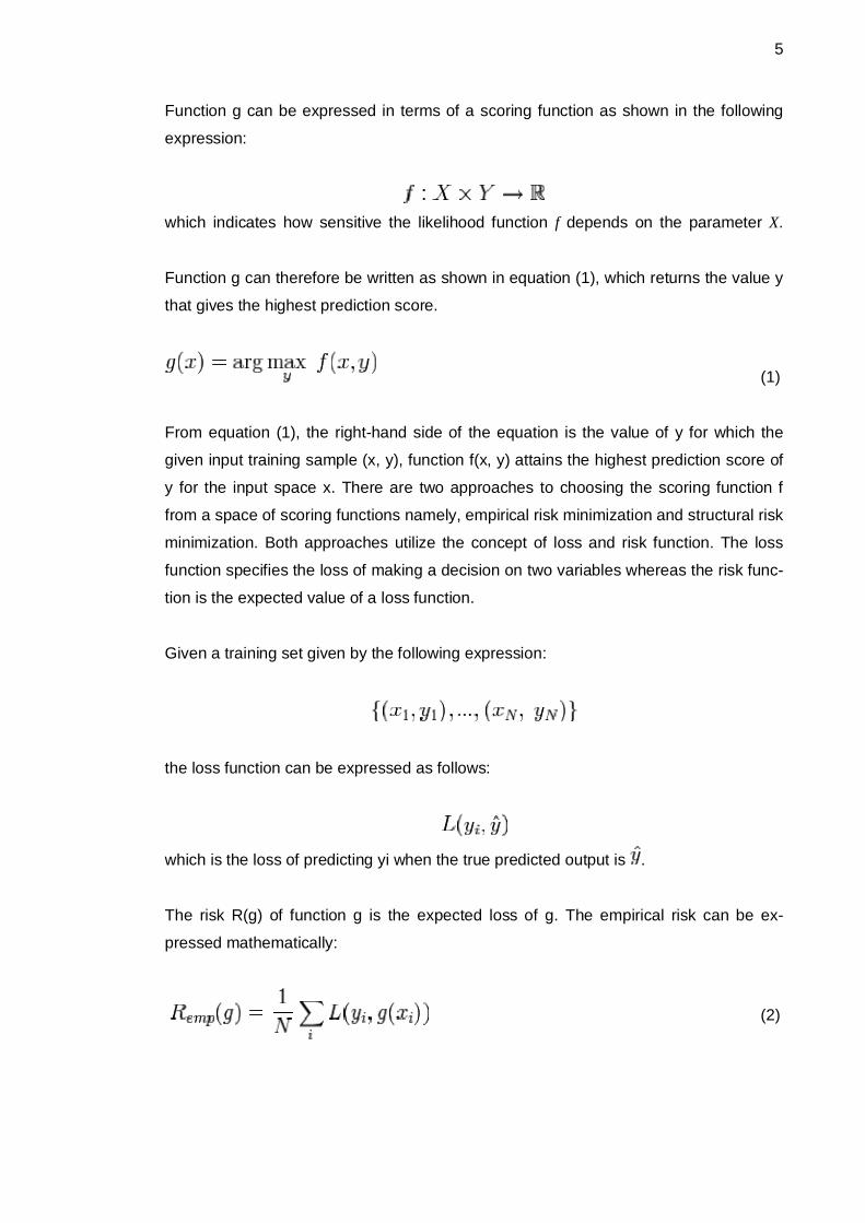
Function g can be expressed in terms of a scoring function as shown in the following

expression:

which indicates how sensitive the likelihood function f depends on the parameter X.

Function g can therefore be written as shown in equation (1), which returns the value y

that gives the highest prediction score.

(1)

From equation (1), the right-hand side of the equation is the value of y for which the

given input training sample (x, y), function f(x, y) attains the highest prediction score of

y for the input space x. There are two approaches to choosing the scoring function f

from a space of scoring functions namely, empirical risk minimization and structural risk

minimization. Both approaches utilize the concept of loss and risk function. The loss

function specifies the loss of making a decision on two variables whereas the risk func-

tion is the expected value of a loss function.

Given a training set given by the following expression:

the loss function can be expressed as follows:

which is the loss of predicting yi when the true predicted output is .

The risk R(g) of function g is the expected loss of g. The empirical risk can be ex-

pressed mathematically:

(2)

6

where the risk is computed over the event space of X and Y. In empirical risk minimiza-

tion, the goal of the supervised learning algorithm is to seek a function g that minimizes

Remp(g). Many learning algorithms such as ID3, C4.5 and CART are probabilistic

whereby the function g can be modelled by equation (3) or the function g can be mod-

elled using a joint probability shown in equation (4).

where x and y are given set of training examples.

When g is modelled by equation (3), the loss function is negative log likelihood as ex-

pressed in equation (5).

Therefore the empirical risk is equivalent to the maximum likelihood estimation (MLE),

which is a method of estimating the parameters of a statistical model. The empirical

risk equation expressed in terms of MLE is shown in equation (6).

Remp(g) = -1/N S log P(yi | xi) (6)

where yi are the class label and xi are the input feature.

For an insufficient training set, the empirical risk minimization produces high variance

and poor generalization which causes overfitting. On the other hand, structural risk

minimization seeks to prevent overfitting caused as a result of generalization from few-

er training samples by incorporating a regularization penalty into the optimization. The

regularization penalty depends on the geometric property of the function. For example,

when function g is a linear function shown in equation (7):

where are the weights or scalar coefficient and xj are the input space features, a

(3)

(4)

(5)

i

(7)

7

regularization penalty which is the squared Euclidean norm of weights can be ex-

pressed as follows:

Therefore supervised learning optimization utilizing structural risk minimization aim to

find the function g that minimizes J(g) expressed in equation (8).

where the parameter l controls the bias-variance tradeoffs, Remp(g) is the empirical risk

and C(g) is the regularization penalty which is the number of non-zeros of from

equation (7) [8] .

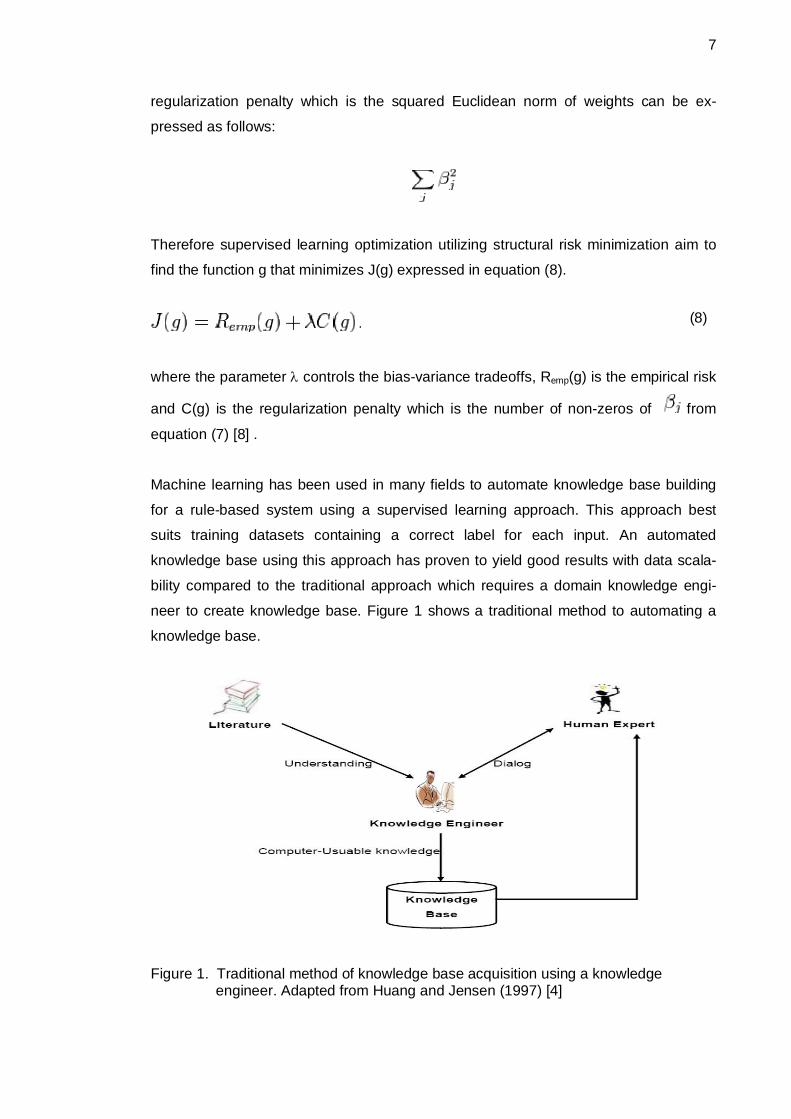
Machine learning has been used in many fields to automate knowledge base building

for a rule-based system using a supervised learning approach. This approach best

suits training datasets containing a correct label for each input. An automated

knowledge base using this approach has proven to yield good results with data scala-

bility compared to the traditional approach which requires a domain knowledge engi-

neer to create knowledge base. Figure 1 shows a traditional method to automating a

knowledge base.

Figure 1. Traditional method of knowledge base acquisition using a knowledge engineer. Adapted from Huang and Jensen (1997) [4]

(8)

8

As illustrated in figure 1, the traditional method approach uses a knowledge engineer

through dialog interaction with a domain human expert in addition to research findings

from literature archives. The information gained by the knowledge engineer is encapsu-

lated into computer-usable knowledge known as rules through the process of inductive

inference mechanism.

The performance of the rules created using this approach is almost accurate but how-

ever this approach scales poorly with an increase in the dataset. The alternative ap-

proach which scales well with increased data size is through a machine-learning ap-

proach. [4]

The machine-learning approach uses a heuristic inductive learning by searching

through the training data to infer facts that can be used for predicting new unseen data.

Figure 2 shows a machine-learning approach using supervised learning.

Figure 2. Machine-learning approach to automated knowledge base building through supervised learning process. Adapted from Huang and Jensen (1997) [4]

As illustrated in figure 2, the domain human expert creates a training dataset which is

used as an input to a machine learning program. The patterns captured from the

dataset are encapsulated in the form of rules used to build a knowledge base. [4]

9

A comprehensive illustration of a supervised learning approach is shown in figure 3.

Raw input data are processed using the feature selection process to reduce the dimen-

sionality of the input data. The processed data is further scaled into training and test

data. A training dataset is used to create a data model and the test data is used to vali-

date the model from unseen data.

Figure 3. Supervised learning. Adapted from Huang and Jensen (1997) [4]

As depicted in figure 3, both training data and test data are sampled from raw data.

The test data is used to validate the model built from the training data and the perfor-

mance of the model can be validated by the profit outcome. The tradeoff for selecting a

learning algorithm depends on speed of training, memory usage, predictive perfor-

mance on new data and interpretability of the algorithm. [3; 4; 6; 8; 9; 14]

2.2 Rule-Based System

A rule-based system also called an expert system, has been defined as follows: “it is

an intelligent computer program that uses knowledge and inference procedures to

solve problems that are difficult enough to require significant expertise”. [29] The main

idea of a rule-based system is to capture the knowledge of a human expert in a spe-

cialized domain into an automated system. The captured knowledge is stored as rules.

10

The main components of a rule-based system are: working memory, inference engine

and a knowledge base. [5]

Figure 4 shows the architecture of a rule-based system

Figure 4: Architecture of a rule-based system. Adapted from JBoss Drools Team [5]

As shown in figure 4, the working memory is a database used to store a collection of

facts known about the domain. The facts can be asserted, modified or retracted from

the working memory. A real world example of facts in a medical domain could be in-

formation of a particular patient being diagnosed, such as age, sex, height, weight and

blood pressure. The knowledge base also known as production memory stores rules

that are used by the inference engine. to match against facts in the working memory.

These sets of rules represent knowledge about the domain. The general syntax of a

rule is of the form

If <condition> THEN <action>

where <condition> also known as antecedent clause is evaluated depending upon the

problem being solved and the <action> also known as consequent clause is used to

manipulate the facts in the working memory. [5]

11

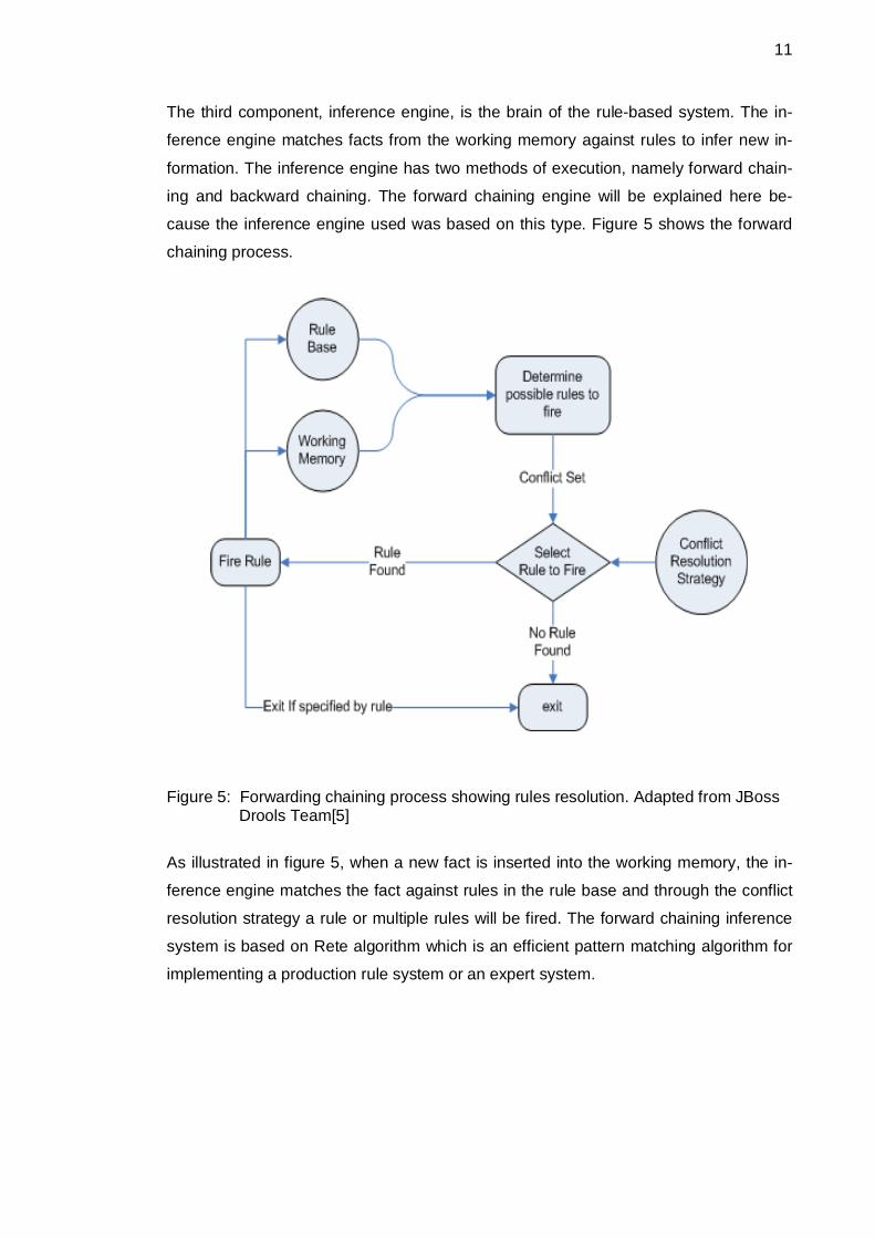
The third component, inference engine, is the brain of the rule-based system. The in-

ference engine matches facts from the working memory against rules to infer new in-

formation. The inference engine has two methods of execution, namely forward chain-

ing and backward chaining. The forward chaining engine will be explained here be-

cause the inference engine used was based on this type. Figure 5 shows the forward

chaining process.

Figure 5: Forwarding chaining process showing rules resolution. Adapted from JBoss Drools Team[5]

As illustrated in figure 5, when a new fact is inserted into the working memory, the in-

ference engine matches the fact against rules in the rule base and through the conflict

resolution strategy a rule or multiple rules will be fired. The forward chaining inference

system is based on Rete algorithm which is an efficient pattern matching algorithm for

implementing a production rule system or an expert system.

12

An illustrative example of a medical diagnosis using forward chaining is shown in list-

ing 1.

Listing 1. Medical diagnosis using forward chaining. Adapted from Dame Team [3]

As illustrated in listing 1, the Rule-Base contains six rules, labelled R1 to R6 and five

facts in the working memory. During the inference engine matching process, the first

rule, R1, is matched against facts in the working memory and since the antecedent part

is not true, R1 is not fired. The next rule in the Rule-Base, R2, is matched against the

facts in the working memory and since the antecedent part of the rule is true, R2 is

fired. Finally the working memory is updated by adding a new fact to the working

memory. Subsequent rules, R3 onward, in the Rule-Base are matched against the

13

facts in working memory until the last rule R1 is fired to predict the diagnosis, after

which the process terminates with no more rules to fire. [3; 5; 11; 23]

2.3 Data Mining

The need to seek patterns in data began long since the evolution of man. For example,

hunters seek patterns in animal migration seasonally, farmers seek pattern in crop

growth and politicians seek pattern in voters’ opinions. In the past few decades, large

amounts of data have been generated from online transactions and from sensors.

These online data sources contain information on economic and financial institutions,

social sciences, sports and entertainment industry. [30] There is therefore a large gap

between data generation and our understanding of the data. Data mining seeks to ex-

tract patterns from data and to transform them into an understandable structure for

application. Two primary goals of data mining tend to be prediction and description.

Prediction involves using feature sets which are obtained from attributes of original

datasets by applying transformation techniques such as reducing the original dimen-

sionality of the data and eliminating noisy or corrupted data. The feature set is used to

predict unknown or future values whereas description focuses on finding patterns de-

scribing the data that can be interpreted by a human. [18, 79]

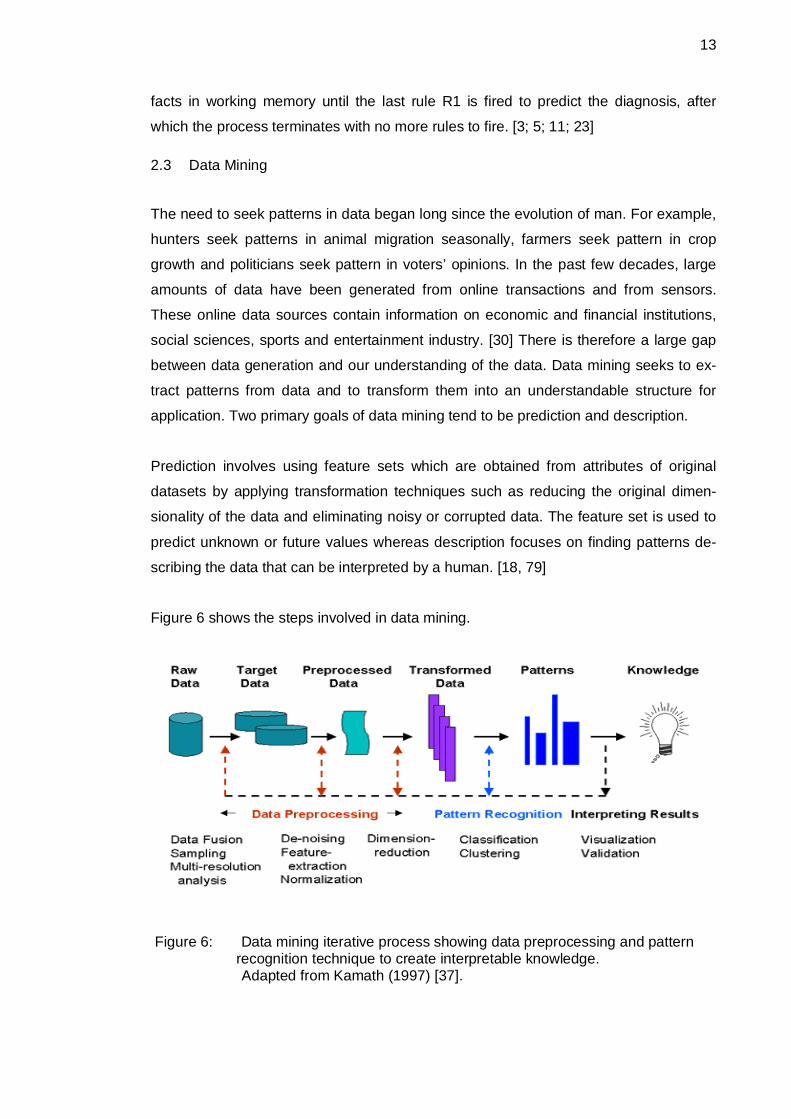
Figure 6 shows the steps involved in data mining.

Figure 6: Data mining iterative process showing data preprocessing and pattern recognition technique to create interpretable knowledge.

Adapted from Kamath (1997) [37].

14

As illustrated in figure 6, data mining is an iterative process involving data prepro-

cessing, pattern recognition and interpretation of results. Data preprocessing involves

steps such as removing noisy and inconsistent data, dimension reduction and pattern

recognition which is achieved by application of different clustering or classification

techniques.

Clustering is a technique used to create subgroups of similar items amongst a large

collection of data. Clustering is a type of classification approach known as unsuper-

vised where the class labels of the data are unknown. The goal of clustering is to cre-

ate similar data into a cluster and dissimilar data into another cluster based on similari-

ty measurement criteria. An example of a clustering algorithm is the k-means which

works by finding k unique clusters. The criterion used in clustering is based on the

mean of the values in the clusters to the cluster centroid. Figure 7 shows a simple k-

means clustering example. [18, 146-150; 31]

Figure 7. K-means clustering showing five clusters and their centroid.Adapted from McCullock (2012) [31]

As illustrated in figure 7, the data sets are grouped into five clusters based on their cen-

troid as depicted in the blue bigger dot. Each grouping is done by computing the mini-

mum Euclidean distance of each data in the cluster to the centroid.

Unlike clustering, classification task starts with a dataset containing class labels or tar-

get labels. The goal of classification is to predict the class label by using sampled data

15

known as training data with known labels through a learning process a classifier is

learned which is used to classify unseen data. Classification using datasets with known

labels is known as supervised learning. Examples of classifiers used in supervised

learning include decision tree, logistic regression and Naïve Bayesian classifier. [32, 3-

12]

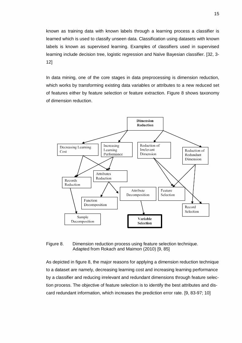
In data mining, one of the core stages in data preprocessing is dimension reduction,

which works by transforming existing data variables or attributes to a new reduced set

of features either by feature selection or feature extraction. Figure 8 shows taxonomy

of dimension reduction.

Figure 8. Dimension reduction process using feature selection technique.Adapted from Rokach and Maimon (2010) [9, 85]

As depicted in figure 8, the major reasons for applying a dimension reduction technique

to a dataset are namely, decreasing learning cost and increasing learning performance

by a classifier and reducing irrelevant and redundant dimensions through feature selec-

tion process. The objective of feature selection is to identify the best attributes and dis-

card redundant information, which increases the prediction error rate. [9, 83-97; 10]

16

There are two approaches to feature selection namely forward and backward selection.

The forward selection method starts with an empty set and sequentially adds the attrib-

ute that best improves the classifier performance until further addition of an attribute

will no longer improve the classifier performance. On the other hand, backward selec-

tion involves starting with all attributes in a dataset and deleting the attribute that best

decreases the classifier performance until further deletion of an attribute does not affect

the performance. [8; 9, 83-97; 10; 14, 29-39; 18, 77-96; 21, 53-85; 24, 100-141, 33]

3 Design and Implementation of the Project

The thesis design illustrated the schematic design process which established the gen-

eral scope and relationships amongst the components. These components included

machine learning and data mining. KNIME software was used to build the thesis design

because KNIME has both machine learning and data mining components integrated

into the software. Using KNIME, a schematic diagram was a created interconnecting

node from both machine learning and data mining that was used to analyze trends in

the datasets and also used to build the prediction models from the training dataset.

The prediction model was used to predict unseen data. Rules were further created from

predicted data which were in the form of “IF THEN” expression. These rules were

served as input to the implementation part of the thesis using Drools Expert, one of the

components of Drools developed by JBoss. Drools Expert was chosen because it uses

rules in the form of “IF THEN” expression to perform reasoning. The implementation

was carried out using the Eclipse integrated development environment. [5]

3.1 Software

The software used in the thesis were Konstanz Information Miner Desktop (KNIME),

Eclipse integrated development environment (IDE) and Astah-professional a unified

modelling language (UML) software. KNIME Desktop is an open-source platform for

data access, data mining, statistics, visualization and reporting. KNIME software pro-

17

vides a rich graphical user interface where processes are created. This thesis devel-

opment was done using the KNIME Desktop with KNIME SDK version 2.7.1.

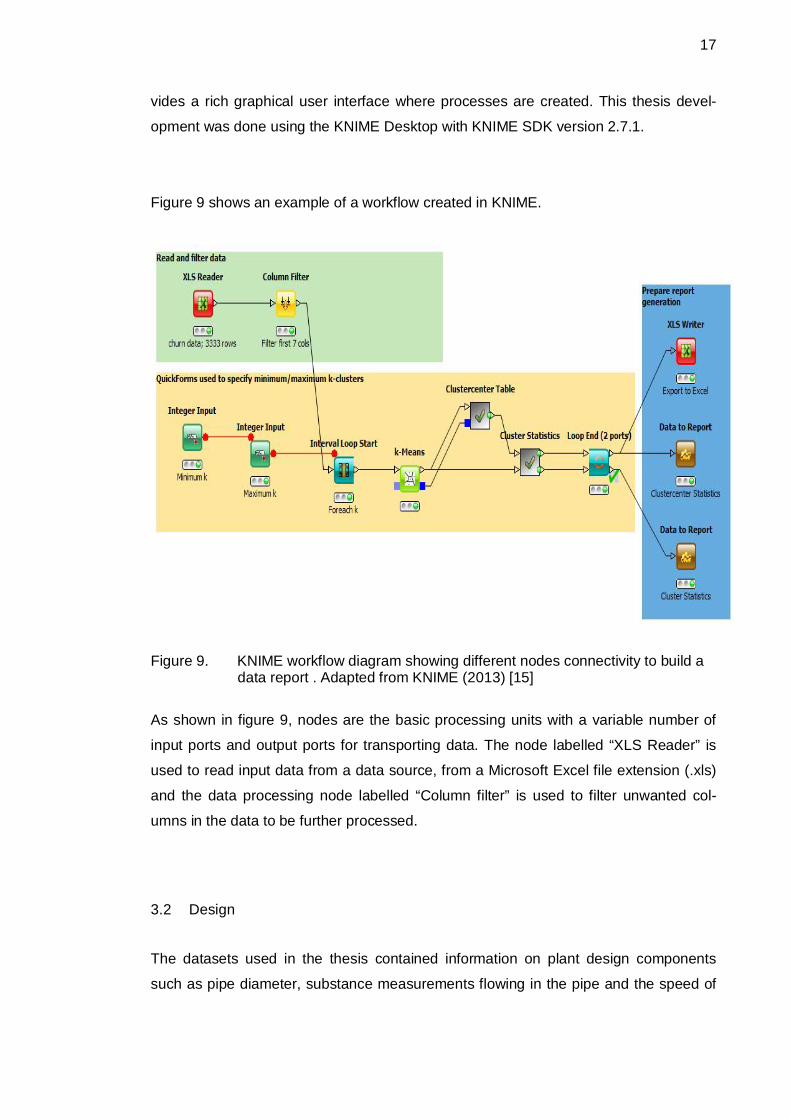
Figure 9 shows an example of a workflow created in KNIME.

Figure 9. KNIME workflow diagram showing different nodes connectivity to build adata report . Adapted from KNIME (2013) [15]

As shown in figure 9, nodes are the basic processing units with a variable number of

input ports and output ports for transporting data. The node labelled “XLS Reader” is

used to read input data from a data source, from a Microsoft Excel file extension (.xls)

and the data processing node labelled “Column filter” is used to filter unwanted col-

umns in the data to be further processed.

3.2 Design

The datasets used in the thesis contained information on plant design components

such as pipe diameter, substance measurements flowing in the pipe and the speed of

18

substance flow in addition to devices such as flow, pressure and temperature sensors.

The datasets comprised attributes and class labels. Attributes are collectively used to

identify a class label. A class label also known as target attribute is the output to each

attributes in a record. For example in medical diagnose data, attributes such as age,

sex or blood pressure can be collectively used to diagnose if a patient is having cancer

or heart attack.

Figure 10. Illustration of attributes and labels in medical diagnosis.

As shown in figure 10, cancer and heart attack are class labels. For example, Patient A

record with attributes such as age with value 45, sex with value female and blood pres-

sure with value 100 is used to the diagnosis of Patient A as having a heart attack.

The thesis dataset comprised 35 column attributes, 12327 rows, 423 class labels and

2335 rows containing one or more missing values. The objectives were to learn a clas-

sifier using training data to build a model. The model was tested against test data and

an acceptable model was chosen to have minimum output performance score of at

least 75%. The model with the best score was further used to predict unseen or new

data. In order to build the model used in prediction, a representational flow diagram

was built. This flow diagram shows the data reading, processing and prediction score.

The thesis data used was in a Microsoft Office Excel comma separated value file

(.csv). The data was read using a file reader, a KNIME processing node for reading

files.

19

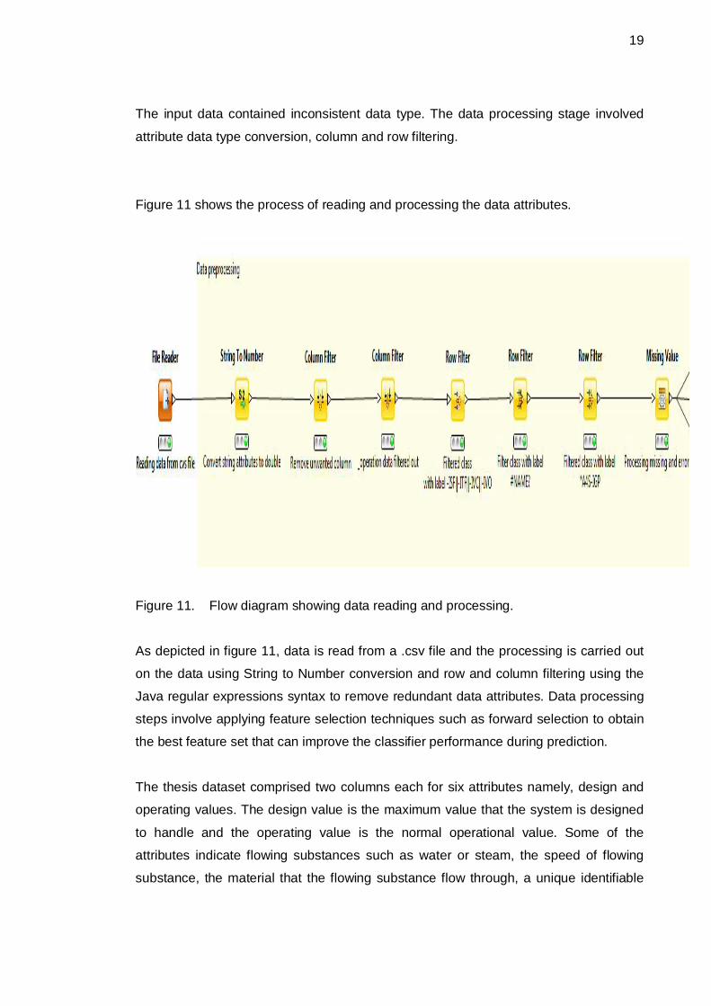
The input data contained inconsistent data type. The data processing stage involved

attribute data type conversion, column and row filtering.

Figure 11 shows the process of reading and processing the data attributes.

Figure 11. Flow diagram showing data reading and processing.

As depicted in figure 11, data is read from a .csv file and the processing is carried out

on the data using String to Number conversion and row and column filtering using the

Java regular expressions syntax to remove redundant data attributes. Data processing

steps involve applying feature selection techniques such as forward selection to obtain

the best feature set that can improve the classifier performance during prediction.

The thesis dataset comprised two columns each for six attributes namely, design and

operating values. The design value is the maximum value that the system is designed

to handle and the operating value is the normal operational value. Some of the

attributes indicate flowing substances such as water or steam, the speed of flowing

substance, the material that the flowing substance flow through, a unique identifiable

20

attribute and a target attribute or class label. Some the attributes contained nominal,

interval and ordinal values. Nominal values have distinct symbols or basically refers to

categorically discrete data. Interval values on the other hand are measured in fixed

equal units whereas ordinal values can be ordered. Detailed information on the

datasets is not shown because of the company sensitive information.

Understanding each attribute values helps to choose appropriate learning algorithms

that can be used for classification. For exampe, JRip and J48 supports a limited

number of dataset attributes with nominal values. During the data processing stages,

15 columns out of the original 35 columns were filtered out. Some of the filtered

attributes contained descriptive information on other attribute columns and some con-

tained the SI unit of other attribute columns. Moreover, the row filtering was further car-

ried out by filtering out the entire row containing target attribute with invalid data. During

the pre-processing stage, one of the exceptions used was ignoring the missing data

from the attribute columns because a huge amount of the data had missing values.

Some of these values could have been accounted for that it was not necessary during

the automation design process. [34]

After the initial data pre-processing stage was performed, the column size was reduced

to 20. Despite the reduction in the column size, the dimensionality was still a problem

because the more features, the higher the computational cost for predictions, which

increases polynomially especially with a large number of class labels. By further em-

ploying the feature selection process, input features with little effect on the output pre-

dictions were removed in order to keep the feature size used by the learning classifier

small, so as to give better prediction performance.

The unique identifiable attribute column was further filtered out because its entries

were unique and it could cause the problem of overfitting by generalization, whereby

the prediction could be finally determined by the unique attribute column. Overfitting

occurs when a learning algorithm produces accurate results on training data but pro-

duces a less accurate performance score when predicting unseen data. An example

could be to predict online shopping behavior on purchasing products. Some of the at-

tributes used in the prediction could be age, size, sex, location or credit card identifica-

tion (ID). Since the credit card ID is unique for each customer, a learning algorithm can

produce 100% prediction performance based on the customer credit card but when

21

given unseen data to the learned classifier, the performance would be less accurate

because the classifier overfitting was a generalization from the credit card attribute.

Moreover, the dataset contained both design and operating values for some attribute

columns. The operating values of the datasets were filtered out. More attribute columns

were filtered out because they had more missing values than actual values. The total

number of columns left after data preprocessing was 7. The dataset is not disclosed

because of the company sensitive information. The remaining dataset that comprised 7

attributes were grouped into three categories and each of these categories was parti-

tioned in the ratio of 85%:15%. The 85% of the data were further partitioned into train-

ing and test sets using relative stratified sampling of which 70% were training sets and

30% test sets. The remaining 15% of the data were used to further validate the perfor-

mance of the learned model.

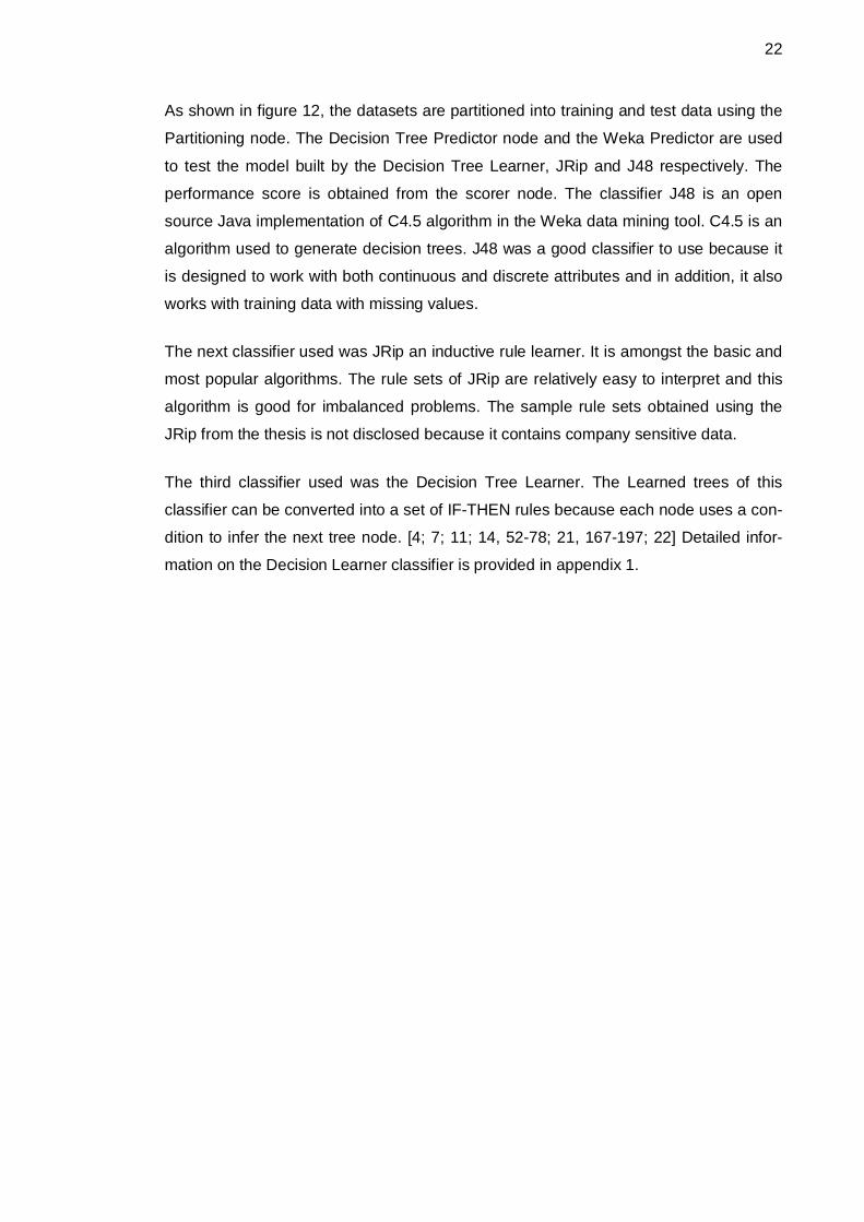
Figure 12. An illustrated diagram showing classifiers, in (a) JRip and J48 and in (b) Decision Tree Leaner used for the data prediction stage.

22

As shown in figure 12, the datasets are partitioned into training and test data using the

Partitioning node. The Decision Tree Predictor node and the Weka Predictor are used

to test the model built by the Decision Tree Learner, JRip and J48 respectively. The

performance score is obtained from the scorer node. The classifier J48 is an open

source Java implementation of C4.5 algorithm in the Weka data mining tool. C4.5 is an

algorithm used to generate decision trees. J48 was a good classifier to use because it

is designed to work with both continuous and discrete attributes and in addition, it also

works with training data with missing values.

The next classifier used was JRip an inductive rule learner. It is amongst the basic and

most popular algorithms. The rule sets of JRip are relatively easy to interpret and this

algorithm is good for imbalanced problems. The sample rule sets obtained using the

JRip from the thesis is not disclosed because it contains company sensitive data.

The third classifier used was the Decision Tree Learner. The Learned trees of this

classifier can be converted into a set of IF-THEN rules because each node uses a con-

dition to infer the next tree node. [4; 7; 11; 14, 52-78; 21, 167-197; 22] Detailed infor-

mation on the Decision Learner classifier is provided in appendix 1.

23

3.3 System Overview Diagrams

The system overview was used to model communication between an actor and the

rule-based system. An actor specifies a role played by a user that interacts with the

rule-based system. Figure 13 shows a use case diagram showing interaction of an ac-

tor with the system.

Figure 13: Use case diagram showing interaction of a user with the rule-based system.

As illustrated in figure 13, the use case illustrates the principal functioning of the sys-

tem where the user logs in to interact with the system. This use case diagram shows a

high-level view of what the rule-based system does and who uses it. For example the

user can log in into the system through a user interface and perform operations such

as verifyDesign and InsertFact and finally log out of the system. [36, 25-41]

In addition to use case diagram, a class diagram was modeled to show the static struc-

ture of the rule-based system. Classes are basic building blocks for class diagrams

24

which show the features of classes, principally the attributes and operations. Attributes

are the properties of a class and operations are the methods or the functionalities of

the class. Figure 14 shows classes interaction in the class diagram.

Figure 14. Class diagram showing association between classes and class interfaces.

As shown in figure 14, there are four classes, Fact, User, InsertFactGUI and Update-

FactGUI. Some of these classes have an inheritance relationship, for example Insert-

FactGUI and UpdateFactGUI inherit a method login from User class. Inheritance is an

object-oriented concept where a class inherits attributes and methods from another

class called a super class. Moreover, UpdateFactGUI class has a composition associa-

25

tion with RuleSession interface. A composition association represents a whole-part

relationship, where in this case the whole object is the RuleSession interface. When

the whole object is deleted, the part object has no meaning. For example, if RuleSes-

sion is deleted, the method readKnowledgeBase can never be executed in Update-

FactGUI class. [36, 47-89]

3.4 Implementation

The language used for the thesis implementation was Java. The application comprised

the following: Runner (Java files) - creates rule packages needed by the inference en-

gine, loads facts into the working memory, load rules, executes inference engine; Rules

– Business logic of the application that contain the production rule. The facts compo-

nents are Plain Old Java Object (POJO) which are ordinary Java Objects with a setters

and getters method. These facts are persisted in a MySQL database for retrieval, dele-

tion and update during execution of the inference engine.

Moreover, production rules were implemented using Drools rule language with an ex-

tension .drl. A rule file, drl file, could have multiple rules, queries and functions in addi-

tion to imports, globals and attributes declarations. A rule starts with the keyword “rule”

followed by the name of the rule in quotes and each rule is terminated with the keyword

“end”. Each rule has an antecedent part preceded by the keyword “when” and a con-

sequence part that is preceded by the keyword “then”. When the antecedent or condi-

tion part is true, the consequence will be executed. The production rules are not dis-

closed because it contains the company sensitive information. Sample rule is shown in

listing 2. [5, 7-35]

rule "rule A"when

$server : Server(processors==4, memory==2048)then

retract($server);end

List 2. Example of a rule declaration.

26

As shown in listing 2, “rule A” is the name of the rule, “$server” is an object instantiation

with two variables “processors” and “memory” and “retract()” method is the action per-

formed on the object “$server”.

The other components of the implementation, loading rules and facts into the inference

involve creating a KnowledgeBase by calling the createKnowledgeBase method.

KnowledgeBase is an interface that manages a collection of rules, processes and in-

ternal types. Since the creation of rules is expensive, the KnowledgeBase stores and

reuses the rules. The KnowledgeBase is further used to create a stateful knowledge

known as StatefulKnowledgeSession which is the main interface for interacting with the

Drools engine. Finally, fireAllRules method is executed to fire a rule or rules that match

with facts in the working memory. [5, 7-35]

Figure 15. A diagram showing how collection of rules in KnowledgePackage and Facts are inserted into the inference engine for rules execution.

As illustrated in figure 15, when rules and facts are inserted into the inference engine

by the StatefulKnowledgeSession, the inference engine determines the set of rules

which can be fired. The fired rules are those with which the antecedent is satisfied.

27

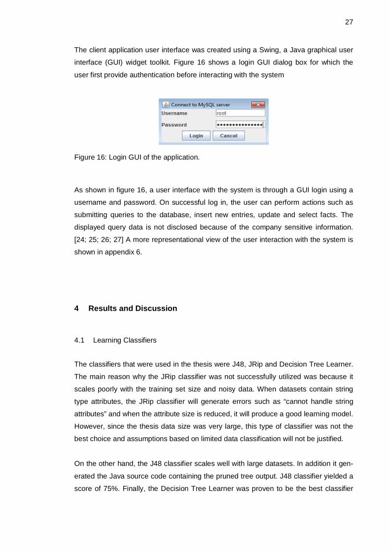
The client application user interface was created using a Swing, a Java graphical user

interface (GUI) widget toolkit. Figure 16 shows a login GUI dialog box for which the

user first provide authentication before interacting with the system

Figure 16: Login GUI of the application.

As shown in figure 16, a user interface with the system is through a GUI login using a

username and password. On successful log in, the user can perform actions such as

submitting queries to the database, insert new entries, update and select facts. The

displayed query data is not disclosed because of the company sensitive information.

[24; 25; 26; 27] A more representational view of the user interaction with the system is

shown in appendix 6.

4 Results and Discussion

4.1 Learning Classifiers

The classifiers that were used in the thesis were J48, JRip and Decision Tree Learner.

The main reason why the JRip classifier was not successfully utilized was because it

scales poorly with the training set size and noisy data. When datasets contain string

type attributes, the JRip classifier will generate errors such as “cannot handle string

attributes” and when the attribute size is reduced, it will produce a good learning model.

However, since the thesis data size was very large, this type of classifier was not the

best choice and assumptions based on limited data classification will not be justified.

On the other hand, the J48 classifier scales well with large datasets. In addition it gen-

erated the Java source code containing the pruned tree output. J48 classifier yielded a

score of 75%. Finally, the Decision Tree Learner was proven to be the best classifier

28

because it scaled well with the training set size and it yielded a score of 92%. [9; 12;

14; 17; 21, 169-198] Detailed information on how these classifiers work and how to

tune the performance is illustrated in appendices 1, 2 and 3.

4.2 Production Rules Generation

The production rules set were obtained from disjoint subsets of the complete data set.

These data sets were partitioned into three categories, data generated by pressure,

temperature and flow sensors. The learned decision trees from the disjoint subsets of

the data were converted into rules and combined into a single rule set. Conflicting rules

from the disjoint subset of the data were resolved before combining them into a single

rule set. Resolving conflicting rules required finding all the rules that had the same an-

tecedent conditions and also attributes that were the same with different continuous

values that differed by no more than 60%.

Another method to resolve conflicting rules is by finding attributes containing an ine-

quality condition having a strictly greater than sign (>) for example, say, Attribute_A >

55 and Attribute_A > 56 then the condition with a smaller continuous value, Attribute_A

> 55, is selected. Likewise, when a rule contains the inequality condition of less than or

equal to (<=), say, Attribute_A <= 55 and Attribute_A <= 56, then the rule with a greater

continuous value, Attribute_A <= 56, will be selected. Conflicted rule sets were kept in

a separate file of conflicting rule set that can further be processed. Non-conflicting rules

were combined into a rule set used to build the knowledge base of the application. [4;

17; 18; 21; 22] Detailed information on how the Decision Learner Trees configuration

was set up is in appendix 1.

4.3 Benefits and Drawbacks

The benefit of using Drools is that it is a declarative style programming approach and it

is easy to understand. Declarative programming expresses logic of a computation

without describing the control flow. This programming style focuses on describing “what

you want to be done” rather than how it is supposed to be done. Compared to other

imperative style languages such as Java and C++, the rules can be easily managed

29

compared to updating a C++ or Java program. Imperative programming however de-

scribes program computation in terms of statements that change the program states,

that is, it focuses on describing “what to do”.

Moreover, the declarative style solution provides improved maintainability. In impera-

tive style programming languages such as C++ and C#, the programming task is al-

ways focused on telling a computer precisely how to do something, the steps to follow

and in what order. Contrary to rule-based system, the task is focused on telling the

computer what you want to be done and the inference engine figures out how it can be

done. This makes rule-based systems more ideal for solving non-algorithmic problems

such as control, classification and decision rules.

Another benefit of using a declarative style solution is that it scales with evolving com-

plexities. It is easier to modify the rule-based system by adding new rules, modify or

remove existing rules compared to updating a Java program. Another benefit of using

the declarative style solution with Drools is its flexibility and performance. The Drools

rule engine is based on the Rete algorithm and it is a generic if-then statement execu-

tor and in addition the Rete algorithm provides Rete node sharing, node indexing and

parallel execution optimization. Using the declarative style solution provides a reusabil-

ity and embedability benefit from its architectural pattern where rules are separated

from the business logic. The Drools application can therefore be embedded (compo-

nent of a program used in another program) into other existing applications.

Some of the drawbacks of using Drools is time investment in training of developers.

The rule base being a critical component of a rule-based system, inefficient rules and

seemingly unpredictable results would affect the complex decisions of a rule-based

system. Another drawback is that rules debugging requires the developer to under-

stand how the underlying system works compared to other imperative languages such

as Java where debugging involves stepping into the code to find the bug. Finally, an-

other drawback of using Drools is its memory consumption because huge amounts of

calculation are cached in order to prevent event reprocessing. [5; 19]

30

4.4 Reliability

The inference mechanisms for decision tree predictions are statistically probabilistic

and therefore the results are not always accurate. [15; 19]

4.5 Further Development

Moreover, this thesis can be further extended to a rule-based web application using the

architecture shown in figure 17.

Figure 17. Rule-based web application architecture. Adapted from Canadas, Palma

and Tunez (2010) [13]

As shown in figure 17, this approach uses Model View Controller (MVC) architecture.

This architectural pattern separates the model, which comprised JavaBean Classes,

the view which comprised JSF and RichFaces pages and the controller which com-

prised Jess.

In this architecture, the model manages the behaviour and data of the application do-

main and it notifies the views and controllers when the state changes. This model class

represents Java EE components, JavaBeans. The view manages the display of infor-

mation and this can be designed using JavaServer Pages (JSP), JavaServer Faces

(JSF) and AJAX which generates dynamic web pages. The controller is used to update

the states of the model. The proposed architecture utilizes a Jess Engine Bean which

31

uses the Jess application programming interface (API) to embed the rule engine into

the architecture. [13]

Furthermore, future work can be done by datasets mapping. The data used comprised

of 6 different thesis datasets from which there were identical class labels for different

thesis datasets. The thesis can be further improved by performing mapping of data

attributes to find a pattern of how the attributes vary from one thesis to another. By per-

forming the mapping, a known pattern can be used to generate a prediction model with

generic rules for the dynamic attributes from one thesis dataset to another instead of

combining the entire datasets.

5 Conclusion

The aim of this thesis was to design and implement a machine learning rule-based ap-

plication for verifying automation systems design. The application stages included a

machine learning and data mining phase for creating production rules and a rule-based

phase for implementation using Drools, a business rule management system with a

forward chaining inference engine developed by JBoss.

A rule-based system also known as an expert system uses knowledge specific to a

problem domain to provide “expert quality” performance in that application area. Some

earlier known applications that had been implemented using a rule-based system was

DENDRAL (1967): determines molecular structure based on mass spectrograms.

This thesis demonstrated a hybrid combination of machine learning and rule-based

system. These technologies can be applied to the dataset created during automation

design process. The dataset comprised information that met the classifier’s characteris-

tics from machine learning techniques, which was used to create rules that encapsulate

human expert domain knowledge. The created rules were further used to implement a

rule-based system. The hybrid combination of a machine learning and rule-based sys-

tem showed to be very applicable to automation design process to help solve problems

such as aiding a less experienced engineer during the design work and reduced work

time in verification designs.

32

References

1 Ajith A. Rule-based Expert Systems [online]. Oklahoma State University;URL: http://www.bhu.ac.in/ComputerScience/vivek/softcomp/fuzzy_chapter.pdf.Accessed 10 October 2012.

2 Rereira F, Mitchell T, Botvinic M. Machine learning classifiers and Fmri: A tutorialoverview [online]. Princeton University: Pittsburg PA; July 2013.URL: http://www.princeton.edu/~fpereira/Presentations/ipam2008.pdf.

Accessed 10 October 2012.

3 Dame Team. Machine learning [online].URL: http://ai-depot.com/Tutorial/RuleBased-Conclusion.html.Accessed 15 October 2012.

4 Huang X, Jensen J R. A machine-learning approach to automated knowledge-base building for remote sensing image analysis with GIS data [online]. Mary-land, United State: The American Society for Photogrammetry & Remote SenS-ing; October 1997.

URL: http://www.asprs.org/a/publications/pers/97journal/october/ 1997_oct_1185-1194.pdf. Accessed 15 October 2012.

5 JBoss Drools Team. Drools Expert User Guide [online]. Community documenta-tion version 5.2.0.Final.URL: http://docs.jboss.org/drools/release/5.2.0.Final/drools-expert-docs/html/.Accessed 20 October 2012.

6 Sasikumar M, Ramani S, Raman S M, Anjaneyulu KSR, Chandrasekar R. APractical Introduction to Rule Based Expert System [online]. Special InterestGroup on Artificial Intelligence. New Delhi, India: Narosa Publishing House; 2007.URL: http://sigai.cdacmumbai.in/files/ESBook.pdf. Accessed 20 October 2012.

7 Hall L O, Chawla N, Bowyer K W. Combining decision trees larned in Parallel[online]. FL, USA: University of Florida; 1998.URL: www3.nd.edu/~dial/papers/DDM98.pdf. Accessed 21 October 2012.

8 The Saylor Foundation. Supervised learning [online]. D.C, Washington: USA:2013.URL: http://www.saylor.org/site/wp-content/uploads/2011/11/CS405-6.2.1.2-WIKIPEDIA.pdf.Accessed 21 October 2012.

33

9 Rokach L, Maimon O. Data Mining and Knowledge Discovery Handbook. 2nd ed.New York: Springer; 2010.

10 Kohavi R, John G H. Wrappers for feature subset selection [online]. Artificial li-gence 97. CA, USA: Elsevier; May 1996.URL: http://ai.stanford.edu/~ronnyk/wrappersPrint.pdf. Accessed 7 November2012.

11 Freeman-Hargis J. Rule-Based Systems and Identification Trees [online]. Artifi-cial Intelligence.URL: http://ai-depot.com/Tutorial/RuleBased.html. Accessed 21 October 2012.

12 Korting T S. C4.5 algorithm and Multivariate Decision Tree [online]. Sao Jose dosCampos, Brazil: Image Processing Division, National Institute for Speech Re-search.URL: http://id3-c45.xp3.biz/dokumentasi/daftar_pustaka/12 C4.5 algorithm andMultivariate Decision Trees.pdf. Accessed 8 November 2012.

13 Canadas J, Palma J, Tunez S. A MDD approach for generating Rule-based WebApplication from OWL and SWRL [online]. Spain: University of Almeria; June2010.URL: http://ceur-ws.org/Vol-604/paper6.pdf. Accessed 14 January 2013.

14 Mitchell T M. Machine Learning. 1st ed. New York, NY: McGraw-Hill; 1997.

15 KNIME [online]. Zurich, Gemany; 2013. URL: http://www.knime.org/knime-applications/churn-analysis. Accessed 15 October 2013.

16 Astah, Astah Community [online]. URL: http://astah.net/editions/community. Accessed 15 November 2012.

17 Rajput A, Aharwal R P. J48 and JRIP Rules for E-Governance Data [online]. In-dia: International Journal of Computer Science and Security; 2011.

URL: http://www.cscjournals.org/csc/manuscript/Journals/IJCSS/ volume5/Issue2/IJCSS-448.pdf. Accessed 18 November 2012.

34

18 Nisbet R, Elder J, Miner G. HANDBOOK OF Statistical Analysis & Data MiningApplications. 1st ed. MA, USA: Elsevier; 2009.

19 Bali M. Drools JBoss Rules 5.0 Developer’s Guide. 1st ed. USA: Packt Publishing;2009.

20 Witten I H, Frank E. DATA MINING Practical Machine Learning Tools and Tech-niques.2nd ed. CA, USA: Elsevier; 2005;

21 Kantardzic M. Concepts, Models, Method, and Algorithms. 2nd ed. NJ, USA:Wiley; 2011;

22 Quinlan J R. Generating Production Rules From Decision Trees [online]. MA,USA: Artificial Intelligence Laboratory Massachusetts Institute of Technology;1987.

URL: http://citeseerx.ist.psu.edu/viewdoc/ download?doi=10.1.1.98.9054&rep=rep1&type=pdf. Accessed 12 December 2012.

23 Chiang A T A, Ku C C. Using knowledge-base intelligent reasoning to supportdynamic collaborative design [online]. USA: National Tsing Hua University; 2004.

URL: http://citeseerx.ist.psu.edu/viewdoc/ download?doi=10.1.1.130.4380&rep=rep1&type=pdf. Accessed 12 December 2012.

24 Alpaydin E. Introduction to Machine Learning. 2nd ed. London, England: MITpress; 2010.

25 Deitel P, Deitel H. Java for Programmers. 2nd ed. Indiana, USA: Pearson Educa-tion, Inc.; March 2012. p318-906.

26 Parsian M. JDBC Recipes A Problem-Solution Approach. 1st ed. CA, USA:Apress; September 2005; p.1-256, p.431-613.

27 Speegle G D. JDBC Practical Guide for Java Programmers. 1st ed. CA, USA:Elsevier Science; August 2002.

28 Pöyry. Virtual MILL [online]. 2013; URL: http://www.virtualmill.poyry.com/index.html. Accessed 1 October 2012.

35

29 Aziz A A, Expert System:PDAMum [online]. 2005. URL: http://www.generation5.org/content/2005/PDAMum.asp. Accesed 21 October 2013.

30 Ma L, Simonoff J S. Links to Useful Data [online]. NY, USA: New York University. URL: http://people.stern.nyu.edu/schatter/datalink.html. Accessed 21.10.2012.

31 McCullock J. Clustering [online]. mnemstudio.org; 2012. URL: http://mnemstudio.org/clustering-k-means-introduction.htm. Accessed 21 October 2013.

32 Harrington P. Machine Learning IN ACTION. 1st ed. NY, USA: Manning Publica-tion Co.; 2012.

33 Jain A K. Feature selection [online]. MI, USA: Michigan State University; 2013. URL: http://www.cse.msu.edu/~cse802/Feature_selection.pdf. Accessed 21 October 2013.

34 Witten I H, Frank E. Data Mining [online]. MD, USA: University of Maryland; 2013.URL: http://www.umiacs.umd.edu/~joseph/classes/459M/year2010/

Chapter2_4-on-1.pdf. Accessed 21 October 2013.

35 MathWorks documentation. Treeprune [online]. MathWorks; 2013. URL: http://www.mathworks.se/help/stats/treeprune.html. Accessed 23 October 2013.

36 Bennett S, Skelton J, Lunn k. UML. 1st ed. Glasgow: Schaum Outline Series;2001.

37 Kamath C. Mining Data for Gems of Information [online]. CA, USA: LawrenceLivermore National Laboratory; 2000.

URL: https://www.llnl.gov/str/Kamath.html. Accessed 10 December 2012

Appendix 1

1 (5)

Decision Trees Learner Configuration

Decision tree is an important form of knowledge representation but however it is not

commonly implemented directly in a rule-based system. The complexity of the tree in-

creases with large datasets which makes it difficult to maintain and update the tree.

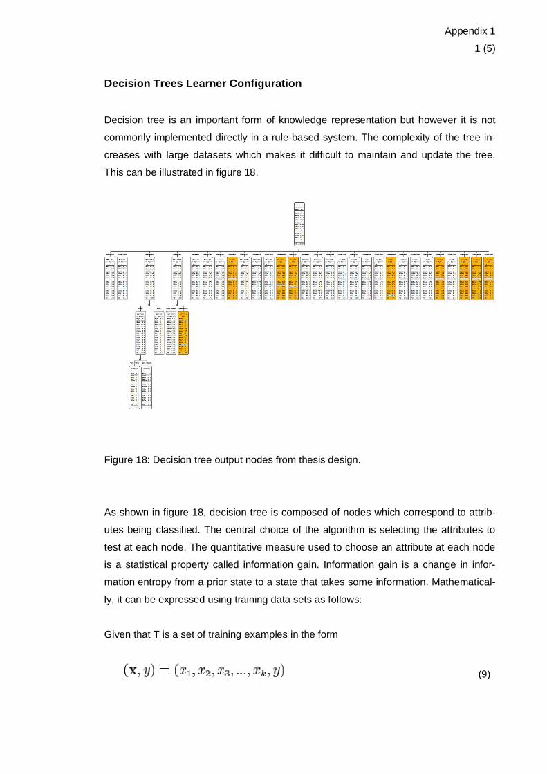
This can be illustrated in figure 18.

Figure 18: Decision tree output nodes from thesis design.

As shown in figure 18, decision tree is composed of nodes which correspond to attrib-

utes being classified. The central choice of the algorithm is selecting the attributes to

test at each node. The quantitative measure used to choose an attribute at each node

is a statistical property called information gain. Information gain is a change in infor-

mation entropy from a prior state to a state that takes some information. Mathematical-

ly, it can be expressed using training data sets as follows:

Given that T is a set of training examples in the form

(9)

Appendix 1

2 (5)

Decision Trees Learner Configuration

where XaÎ vals(a), value of the ath attribute of sample X and y is the corresponding

class label. The information gain for attribute a is therefore shown in equation (10).

Attribute with the highest information gain will therefore be used as the root node in the

decision tree. The process of selecting new attribute and partitioning, the branch node

from the root node, repeats until every attribute has been used.

The Decision Tree Learner configuration used in the thesis is shown in figure 19.

Figure 19: Decision Tree Learner configuration.

As illustrated in figure 19, the Class column contained the class label to be predicted.

The quality measured used was Gini index that measures how equitable a resource is

(10)

Appendix 1

3 (5)

Decision Trees Learner Configuration

distributed in a population. It is the difference between a theoretical equality of some

quantity and the actual value over a range of related variable. It can be represented

mathematically as shown in equation (11) and the evaluation criterion for selecting an

attribute, ai is shown in equation (12).

On the other hand, the gain ratio can be expressed mathematically as shown in equa-

tion (13):

Gain ratio therefore favours attributes for which the denominator is very small. This

quality measure biases decision tree against attributes with large number of distinct

values. One of the drawbacks of gain ratio is that it prefers unbalanced splits whereas

Gini index biases towards multivalued attributes and also with large number of classes,

the quality measure decreases. Gini index quality measure gave a performance score

of 82% compared to 72% performance score using gain ratio.

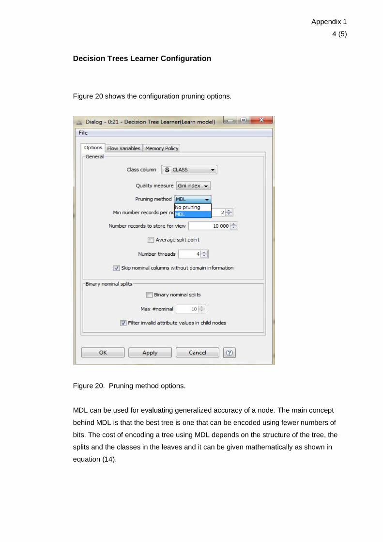
The next configuration option was pruning method which is a technique in machine

learning that reduces the error and complexities of induced trees. Pruning avoids over-

fitting which increases the generalization performance and the prediction quality. The

method options were minimum description length (MDL) and no pruning.

(12)

(11)

(13)

Appendix 1

4 (5)

Decision Trees Learner Configuration

Figure 20 shows the configuration pruning options.

Figure 20. Pruning method options.

MDL can be used for evaluating generalized accuracy of a node. The main concept

behind MDL is that the best tree is one that can be encoded using fewer numbers of

bits. The cost of encoding a tree using MDL depends on the structure of the tree, the

splits and the classes in the leaves and it can be given mathematically as shown in

equation (14).

Appendix 1

5 (5)

Decision Trees Learner Configuration

where St denotes instances that have reached node t. Since the datasets contained

noisy data, this method was chosen compared to the option of no pruning where by

noisy data can affect the overall performance.

Moreover, Min number of records per node used was 2 and the number of records to

store view was set to 10000 because of the size of the attributes; Average split point

was set to default, whereby the split value for numeric attributes is determined accord-

ing to the mean value of the two attribute values that separate the two partitions; Num-

ber of threads set to default processors or cores that are available in KNIME; The other

options such as skip nominal columns without domain information, binary nominal

splits, max #nominal and filter invalid attribute values in child nodes which can be used

to tune the performance of the decision tree on attributes with nominal values. [7; 9; 14,

20]

(14)

Appendix 2

1 (2)

J48 Classifier Configuration

J48 decision tree classifier is Waikato Environment for Knowledge Analysis (Weka)

optimized implementation of C4.5. Weka is an open-source machine learning software

developed at University of Waikato.

Figure 21 shows the configuration of J48 decision tree classifier.

Figure 21: J48 classifier configuration

As illustrated in figure 21, there are 12 options to configure the classifier. The bi-

narySplits option is set to false otherwise setting to true will set binary splits on nominal

attributes when building the trees.

The next option is the confidenceFactor which is set to 0.25. It ranges from 0 to 1 and

the smaller the confidence factor used the higher the tree pruning. The debug option is

Appendix 2

2 (2)

J48 Classifier Configuration

set to false in order not to output classifier info to the console every run of the classifier.

The next option is minNumObj which specifies the minimum number of instances per

leaf. The option numFolds is used to determine the amount of data used for reduced-

error pruning. The numFolds is set to 3 where one fold is used for pruning the two

folds for tree growing. Option reducedErrorPruning is set to true because of its simplici-

ty and speed with respect to the datasets used in the thesis. The options saveIn-

stanceData, unprunned, useLaplace all set to false and the seed used randomizing the

data is set to 1. Depending on the datasets, these options can be fine tuned to yield

different optimal solution.

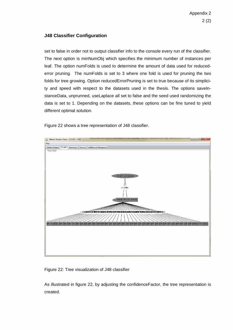
Figure 22 shows a tree representation of J48 classifier.

Figure 22: Tree visualization of J48 classifier

As illustrated in figure 22, by adjusting the confidenceFactor, the tree representation is

created.

Appendix 3

1 (2)

JRip Configuration

JRip implements a propositional rule learner, Repeated Incremental Pruning to Pro-

duce Error Reduction (RIPPER). A detail algorithm for RIPPER adapted from KNIME is

outlined as follows:

Initialize RS = {}, and for each class from the less prevalent one to the more frequent

one, DO:

1. Building stage:

Repeat 1.1 and 1.2 until the description length (DL) of the ruleset and examples is 64

bits greater than the smallest DL met so far, or there are no positive examples, or the

error rate >= 50%.

1.1. Grow phase:

Grow one rule by greedily adding antecedents (or conditions) to the rule until the rule is

perfect (i.e. 100% accurate). The procedure tries every possible value of each attribute

and selects the condition with highest information gain: p(log(p/t)-log(P/T)).

1.2. Prune phase:

Incrementally prune each rule and allow the pruning of any final sequences of the an-

tecedents; The pruning metric is (p-n)/(p+n) -- but it's actually 2p/(p+n) -1, so in this

implementation we simply use p/(p+n) (actually (p+1)/(p+n+2), thus if p+n is 0, it's 0.5).

2. Optimization stage:

After generating the initial ruleset {Ri}, generate and prune two variants of each rule Ri

from randomized data using procedure 1.1 and 1.2. But one variant is generated from

an empty rule while the other is generated by greedily adding antecedents to the origi-

nal rule. Moreover, the pruning metric used here is (TP+TN)/(P+N).Then the smallest

possible DL for each variant and the original rule is computed. The variant with the

minimal DL is selected as the final representative of Ri in the ruleset. After all the rules

in {Ri} have been examined and if there are still residual positives, more rules are gen-

erated based on the residual positives using Building Stage again.

Appendix 3

2 (2)

JRip Configuration

3. Delete the rules from the ruleset that would increase the DL of the whole ruleset if it

were in it and add resultant ruleset to RS.

Figure 23 shows the dialog option diagram for configuring the classifier.

Figure 23: JRip dialog configuration diagram.

As illustrated in figure 23, checkErrorRate is set to true where the stopping condition is

for error rate >= ½. The option debug is set to false to avoid classifier info display at

console; folds set to 3 from which one fold is used for pruning and two folds for tree

growing; the minimum total weight of instance in a rule is set with option minNo to a

value of 2; the number of optimization runs is set to 2; the seed used to randomize the

data is set to 1 and pruning option usePruning set to true. [9; 12; 14; 21]

Appendix 4

1 (5)

Dataset Row Filtering into Three Categories

Figure 24. Row filter of temperature data into TT category.

Figure 25. Row filtering of temperature data into TI category.

Appendix 4

2 (5)

Dataset Row Filtering into Three Categories

Figure 26. Row filtering of temperature data into TE category.

Figure 27. Row filtering of flow data into FT category.

Appendix 4

3 (5)

Dataset Row Filtering into Three Categories

Figure 28. Row filtering of flow data into FI category.

Figure 29. Row filtering of flow data into FE category.

Appendix 4

4 (5)

Dataset Row Filtering into Three Categories

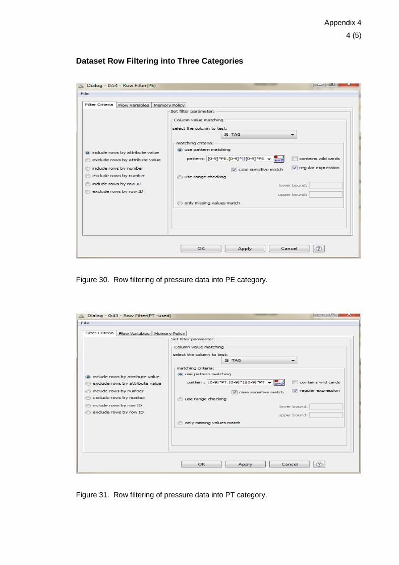
Figure 30. Row filtering of pressure data into PE category.

Figure 31. Row filtering of pressure data into PT category.

Appendix 4

5 (5)

Dataset Row Filtering into Three Categories

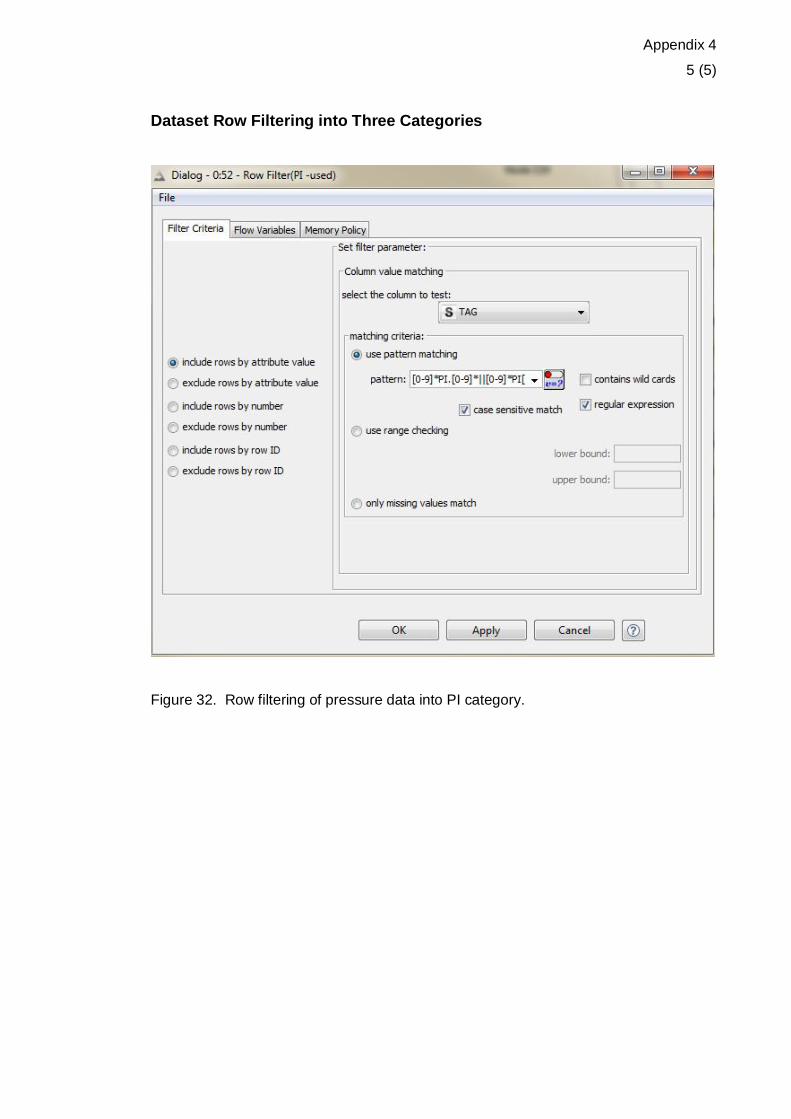
Figure 32. Row filtering of pressure data into PI category.

Appendix 5

1 (1)

Software code

insertIntoInferenceEngine.addActionListener( new ActionListener(

){

@Override

public void actionPerformed( ActionEvent e ){

try {

// load up the knowledge base

knowledgeBase = readKnowledgeBase( );

ksession = knowledgeBase.newStatefulKnowledgeSession( );

logger = KnowledgeRuntimeLoggerFactory.newFileLogger( kses-

sion, "logfile" );

Facts fact = new Facts( );

fact.setDn( Double.parseDouble( dnTextField.getText( ) ) );

fact.setId( Integer.parseInt( idTextField.getText( ) ) );

fact.setFlowcode( flowcodeTextField.getText( ) );

fact.setParentType( parent_typeTextField.getText( ) );

fact.setTempDesign( Double.parseDouble(

temp_designTextField.getText( ) ) );

fact.setPressureDesign( Double.parseDouble( pres-

sure_designTextField.getText( ) ) );

fact.setPipeclass( pipeclassTextField.getText( ) );

fact.setWinnerClass( winnerClassTextField.getText( ) );

ksession.insert( fact );

JOptionPane.showMessageDialog( null, " Facts successfully in-

serted into Working Memory" );

ksession.fireAllRules( );

logger.close( );

} catch ( Throwable t ) {

t.printStackTrace( );

}

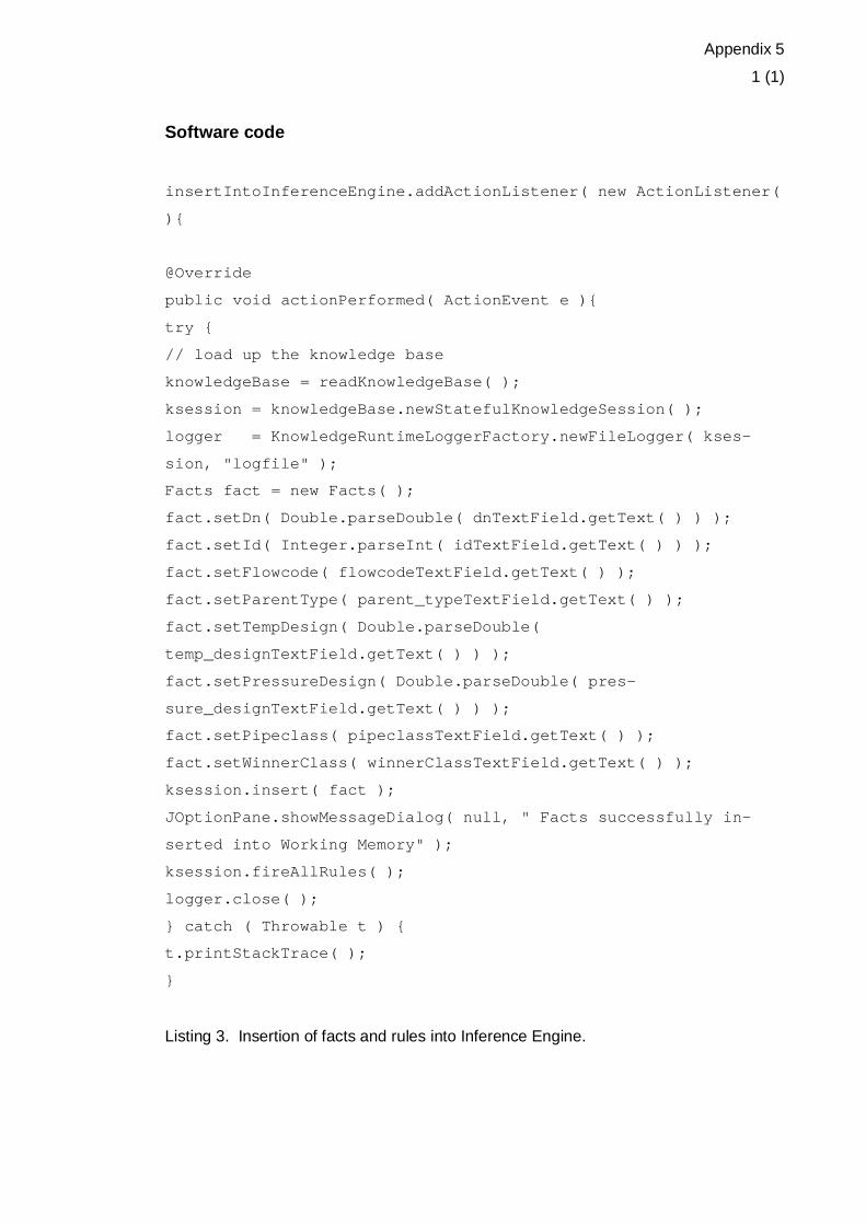
Listing 3. Insertion of facts and rules into Inference Engine.

Appendix 6

1 (2)

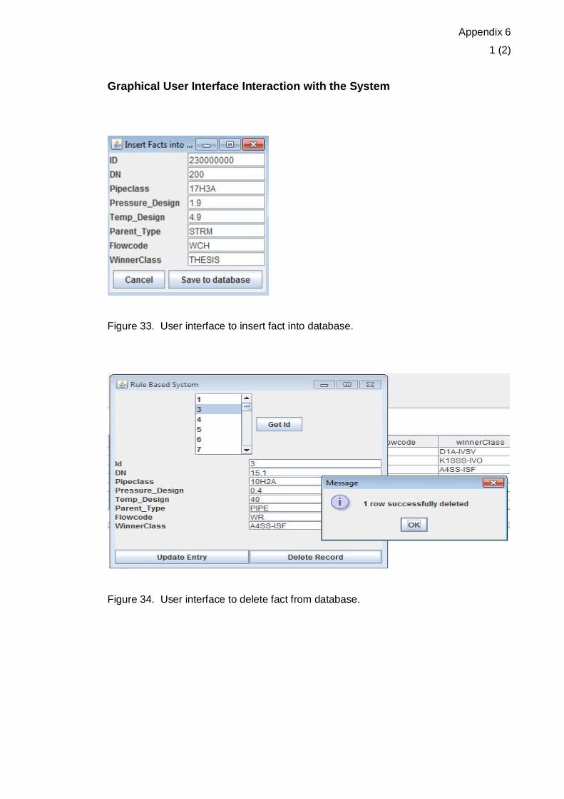
Graphical User Interface Interaction with the System

Figure 33. User interface to insert fact into database.

Figure 34. User interface to delete fact from database.

Appendix 6

2 (2)

Graphical User Interface Interaction with the System

Figure 35. UI to select fact from database to insert into inference engine.

Figure 36. UI showing predicted label after fact is inserted in inference engine.

Appendix 7

1 (1)

Pöyry Virtual Mill§

Figure 37. Pöyry Virtual Mill. Adapted from [28]

As illustrated in figure 37, the Virtual Mill consist of a 3D model for design, a database

for storing and maintaining design data and documents that contain technical infor-

mation.

Pöyry Virtual Mill Concept comprise of 5 tools namely: ProElina, Jalina, UserReports,

MoDeAcad and WebPub. ProElina stores functional and technical information on pro-

cesses, equipments such as pressure vessels, tanks, pipes and operation. Jalina tool

is used for document browsing, creation and editing. The UserReport offers a flexible

report design environment for creating and maintaining reports. WebPub is a web-

based interface to the Virtual Mill, for browsing plant information and last MoDeAcad, a

set of applications namely: process, mechanical, electrical, automation and HVAC en-

gineering for creating 2D documents. [28]