DISCUSSION PAPER SERIES

ABCD

No. 10542  

DYNASTIC INEQUALITY, MOBILITY AND EQUALITY OF OPPORTUNITY 

 Ravi Kanbur and Joseph E Stiglitz 

  

   DEVELOPMENT ECONOMICS and PUBLIC ECONOMICS 

ISSN 0265-8003

DYNASTIC INEQUALITY, MOBILITY AND EQUALITY OF OPPORTUNITY 

Ravi Kanbur and Joseph E Stiglitz 

 Discussion Paper No. 10542 

April 2015 Submitted 01 April 2015 

Centre for Economic Policy Research 

77 Bastwick Street, London EC1V 3PZ, UK 

Tel: (44 20) 7183 8801 

www.cepr.org 

This  Discussion  Paper  is  issued  under  the  auspices  of  the  Centre’s  research programme in DEVELOPMENT ECONOMICS and PUBLIC ECONOMICS.    Any opinions expressed here are those of the author(s) and not those of the Centre for Economic Policy Research. Research disseminated by CEPR may include views on policy, but the Centre itself takes no institutional policy positions. 

The Centre for Economic Policy Research was established in 1983 as an educational charity, to promote independent analysis and public discussion of open economies and  the  relations among  them.  It  is pluralist and non‐partisan, bringing economic research to bear on the analysis of medium‐ and long‐run policy questions.  

These Discussion Papers often represent preliminary or incomplete work, circulated to encourage discussion and comment. Citation and use of such a paper should take account of its provisional character. 

Copyright: Ravi Kanbur and Joseph E Stiglitz

DYNASTIC INEQUALITY, MOBILITY AND EQUALITY OF OPPORTUNITY†

 

Abstract 

One often heard counter to the concern on rising income and wealth inequality is that it is wrong  to  focus on  inequality of outcomes  in a “snapshot.”  Intergenerational mobility and “equality of opportunity”, so the argument goes, is what matters for normative evaluation. In response to this counter, we ask what pattern of  intergenerational mobility  leads to  lower inequality not between individuals but between the dynasties to which they belong? And how does  this pattern  in  turn  relate  to  commonly held  views on what  constitutes  equality of opportunity? We revive and revisit here our earlier contributions which were in the form of working papers (Kanbur and Stiglitz (1982, 1986) in order to engage with the current debate. Focusing  on  bistochastic  transition matrices  in  order  to  hold  constant  the  steady  state snapshot income distribution, we develop an explicit partial ordering which ranks matrices on the criterion of inequality between infinitely lived dynasties. A general interpretation of our result is that when comparing two transition matrices, if one matrix is “further away” from the identity matrix then it will lead to lower dynastic inequality. More specifically, the result presents a computational procedure to check  if one matrix dominates another on dynastic inequality. We  can  also  assess  “equality  of  opportunity”,  defined  as  identical  prospects irrespective of starting position. We find that this is not necessarily the mobility pattern which minimizes dynastic inequality. 

JEL Classification: D31 and D63 Keywords:  dynastic inequality, equality of opportunity, inequality and mobility 

Ravi Kanbur   sk145@cornell.edu Cornell University and CEPR  Joseph E Stiglitz   jes322@columbia.edu Columbia University   

† We first started thinking about this issue in Oxford more than thirty years ago (see Kanbur and Stiglitz (1982, 1986). We have returned to that line of enquiry and are reviving our earlier work given the recent tendency to counter rising inequality concerns with the argument that what matters is not inequality but mobility.

4

1. Introduction

It is clear that global economic forces are now aligned to produce rising income and

wealth inequality. There is, of course, disagreement about the relative importance of the

potential drivers of these changes. The direction of technical change appears to be favoring

capital over labor and, within labor, skilled labor over unskilled labor. Globalization of

trade and investment is transmitting these forces to all countries, and may itself be a

contributor to growing inequality. Across a wide spectrum of countries, there has been an

increase in market power at least in certain sectors, and arguably, more broadly in rent

seeking.1 In Latin America these underlying forces have been countered by pro-active

policy. But elsewhere, including in Asia, Europe and the US, policy has not countered, and

perhaps has even exacerbated, the forces for rising inequality. Not surprisingly, rising

inequality is now of great concern to policy makers and the general public the world over.

The phenomenal response to the book on inequality by Thomas Piketty (2014) is but one

illustration of these concerns.

One often heard counter to the concern on rising inequality is that it is wrong to

focus on inequality of outcome in a “snapshot.” What is important is how income or wealth

evolves over time, especially across generations2. Intergenerational mobility, so the

argument goes, is what matters for normative evaluation. These arguments have resurfaced

in the post-Piketty debates, but have actually been ever present in the discourse on

1 See Stiglitz (2013). 2 Some have argued that inequalities in life time incomes is much less than inequalities observed at any moment of time: in any particular year, some individuals may have a high income, others a low income, but these average out over time. Arguing that consumption is related to permanent income, some, looking at the variability of consumption, suggest that the variability of permanent income must be much lower than the variability in outcomes in any one year. Data before the crisis for the US contaminates the analysis, since a large fraction of Americans in the bottom 80% seemingly believed that they had a much higher permanent income than they did. In any case, this theoretical paper can be made to apply to either context, with an important distinction made below.

5

inequality and public policy. Thus Friedman (1962) writes as follows in Capitalism and

Freedom:

“Consider two societies that have the same annual distribution of income. In one

there is great mobility and change so that the positions of particular families in the income

hierarchy varies widely from year to year. In the other there is great rigidity so that each

family stays in the same position year after year. The one kind of inequality is a sign of

dynamic change, social mobility, equality of opportunity; the other, of a status society. The

confusion between the two kinds of inequality is particularly important precisely because

competitive free enterprise capitalism tends to substitute the one for the other.”

Friedman (1962) uses the phrase “equality of opportunity” which has also received

a great deal of attention in recent years. Roemer (1998), in particular, has attempted to

formalize the concept by distinguishing between two types of factors to which snapshot

inequality might be attributed—circumstances and effort. Circumstances are those factors

which are outside the individual’s control and effort is the term for those factors for which

society holds the individual responsible. A move towards equality of opportunity would

reduce the influence of circumstances on outcome.

Whether one can separate out circumstances from effort, empirically or even

perhaps conceptually, is a live debate (see Arneson (2014), Kanbur and Wagstaff (2014)).3

3 However, both at the theoretical and at the empirical level, both in normative and descriptive models, there is much discussion of the links between inequality of outcomes and inequality of opportunity. While the theoretical work describes mobility in terms of transition matrices (the likelihood of moving from one income level to another), empirical work focuses on correlations, typically simple correlations between the income of a child and the income of the parent(s).

6

But in an intergenerational context Roemer’s (1998) concept has had many precursors.

Thus Nancy Stokey (1998) writes as follows:

“But we care about the sources of inequality as well as its extent, which is why we

distinguish between equal opportunity and equal outcomes. To what extent is the claim that

our society provides equal opportunity justified? How can we tell?....I am going to take the

position that if economic success is largely unpredictable on the basis of observed aspects

of family background, than we can reasonably claim that society provides equal

opportunity. There still might be significant inequality in income across individuals, due to

differences in ability, hard work, luck, and so on, but I will call these unequal outcomes.

On the other hand, if economic success is highly predictable on the basis of family

background, then I think it is difficult to accept the claim that our society provides equal

opportunity. In this case accidents of birth-- unequal opportunity--are primary determinants

of economic status….Consequently, on a first pass we can judge whether there is equal

opportunity by looking at parents and their children to see whether the economic success of

the children is determined in large part by the success of their parents.”

Whether current inequality in turn influences intergenerational mobility is an

important question, as discussed in the recent review by Corak (2013), and by Roemer in

applying his distinction between circumstances and effort to the intergenerational context

(Roemer, 2004).4 But the other side of the causal link is equally important: whether less

mobility leads to more inequality in the next generation. There could be an adverse

feedback process, where more inequality today leads to less mobility, and that in turn leads

to still more inequality in the subsequent generation, and so forth. There is now

considerable evidence of the existence of a correlation between a simple measure of 4 There is now a growing literature in this vein; see Aaberge, Mogstad and Peragine (2011).

7

mobility (intergenerational correlations) and a simple measure of inequality of outcomes

(Gini coefficient); and there is some literature arguing that there is evidence for both parts

of the causal structure.

This paper, by contrast, focuses largely on normative issues, but underneath these

normative issues are complicated relationships between mobility and observed outcomes.

We wish to know whether, for instance, societies with more mobility necessarily have a

higher level of social welfare, using the economists' standard welfare framework.5 Within

such a normative framework, Stokey (1998) and Friedman (1962) seem to suggest that

societies with more mobility have higher levels of social welfare, regardless of what the

degree of inequality in outcomes observed at any moment of time. To evaluate such claims,

one needs to have a more general understanding of both what we mean by more mobility

and an explicit normative framework. Well before Stokey (1998), Atkinson (1981a,

1981b) had characterized equality of opportunity in terms an intergenerational transition

probability matrix with identical rows, and Shorrocks (1978) had referred to this zero

correlation between parents’ income and children’s prospects as “perfect mobility.”

Atkinson and Shorrocks, and others, had also noted an alternative type of transition matrix

which might capture the notion of high mobility, namely one with strong negative

correlation between parents’ income and children’s expected prospects, and Shorrocks

(1978) noted that these two views—“equality of opportunity” and “negative correlation”—

were not necessarily consistent with each other.

5 Of course, many would claim that the economists' standard framework, generalizations of utilitarianism, is badly flawed. We care about fairness, and fairness is defined by equality of opportunity. In this view, equality of opportunity is a value in its own right. We will not have anything more to say on this alternative framework here.

8

We can of course make a direct set of arguments favoring one of these views, and

some of the literature does this.6 But much of the literature relates views on

intergenerational mobility to specific social welfare functions, on the grounds that this

allows precision on the nature of the value judgments in play. Starting from the early work

of Atkinson (1981a, 1981b), and Atkinson and Bourguignon (1982) there is now a very

large literature in this vein. Our earlier working papers, Kanbur and Stiglitz (1982, 1986)

were in this strand of literature, with a particular focus on dynastic inequality. Since those

papers, the literature has seen tremendous growth.7 However, the particular result and

characterization we presented then has not been covered in this literature, and we are

reviving our earlier work in this paper to engage with the current debate on mobility as a

normative counter to inequality. In particular, we wish to ask, what pattern of

intergenerational mobility leads to lower inequality not between individuals but between

the dynasties to which they belong? And how does this pattern in turn relate to commonly

held views on what constitutes equality of opportunity?

The plan of the paper is as follows. Section 2 introduces the notation of

intergenerational transition matrices, and reviews the basic literature to set up the analytical

problem we are addressing. Section 3 presents a characterization result which allows a

partial ordering on intergenerational mobility matrices with respect to dynastic inequality.

Section 4 interprets and discusses the result through particular examples. Section 5

concludes with an agenda for future research.

6 Thus “equality of opportunity” type characterizations have been appealed to directly by Roemer (1998) and by the earlier literature of which Dworkin (1981) is a prime example. 7 Comprehensive surveys of the earlier literature include the one by Fields and Ok (1999). Examples of papers in this vein include Markandya (1984), Chakravarty, Dutta and Weymark (1985) and Dardanoni (1993). More recent references are given in Corak (2013) and in Amiel et. al. (2013).

9

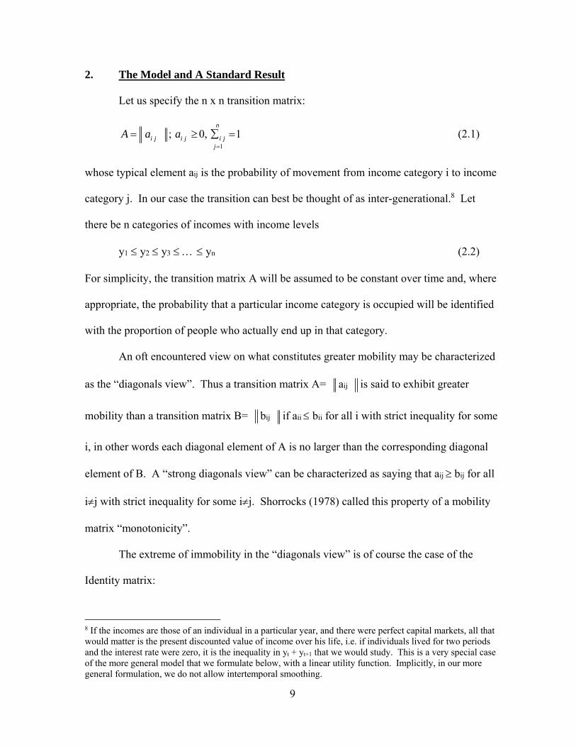
2. The Model and A Standard Result

Let us specify the n x n transition matrix:

1

; 0, 1n

i j i j i jj

A a a

(2.1)

whose typical element aij is the probability of movement from income category i to income

category j. In our case the transition can best be thought of as inter-generational.8 Let

there be n categories of incomes with income levels

y1 y2 y3 yn (2.2)

For simplicity, the transition matrix A will be assumed to be constant over time and, where

appropriate, the probability that a particular income category is occupied will be identified

with the proportion of people who actually end up in that category.

An oft encountered view on what constitutes greater mobility may be characterized

as the “diagonals view”. Thus a transition matrix A= aij is said to exhibit greater

mobility than a transition matrix B= bij if aii bii for all i with strict inequality for some

i, in other words each diagonal element of A is no larger than the corresponding diagonal

element of B. A “strong diagonals view” can be characterized as saying that aij bij for all

ij with strict inequality for some ij. Shorrocks (1978) called this property of a mobility

matrix “monotonicity”.

The extreme of immobility in the “diagonals view” is of course the case of the

Identity matrix:

8 If the incomes are those of an individual in a particular year, and there were perfect capital markets, all that would matter is the present discounted value of income over his life, i.e. if individuals lived for two periods and the interest rate were zero, it is the inequality in yt + yt+1 that we would study. This is a very special case of the more general model that we formulate below, with a linear utility function. Implicitly, in our more general formulation, we do not allow intertemporal smoothing.

10

1

;0ij ij

for i jA I a

for i j

(2.3)

In this case, families' status remains unchanged generation after generation. Strong

monotonicity simply means that there is a smaller probability of remaining in the same

position, and a higher probability of going into every other position.

The other extreme is sometimes argued to be the matrix which has ones along the non-

leading diagonal and zero’s elsewhere:

; ij ijA K a k 1 1

0 1

for j n i

for j n i

(2.4)

Atkinson (1981a) calls this the case of “complete reversal”. Those at the bottom move to

the top and vice versa. Atkinson contrasts this with another view of perfect mobility,

namely that of “equality of opportunity” as indicated by independence of future prospects

from the current situation. This is given by a matrix whose rows are identical

E =

a

a

a

(2.5)

Where a

represents the vector of transition probabilities, identical for every initial state.

Shorrocks (1978) also uses (2.5) to define his property PM (“perfect mobility”). As

Shorrocks goes on to show, one cannot both hold the “diagonals view” and the “equality of

opportunity view” simultaneously. For example, with

A = 0 1

1 0

and B =½ ½

½ ½

(2.6)

11

it should be clear that A is better than B on the diagonals view while the reverse is true on

the equality of opportunity view. This disjuncture came to be well appreciated in the

technical literature which developed since the work of Shorrocks and Atkinson (see for

example the survey by Fields and Ok (1999)), and yet one finds both views present in the

discourse on intergenerational mobility.

There has been considerable development in the literature through specification of

explicit dynastic social welfare functions. Consider a two period world with dynasty i

currently having income yi. Thus income in the next period is yj with probability aij, from

(2.1). If W(yi,yj) represents the welfare from incomes (yi,yj), then the expected welfare of

dynasty i is9

Vi = 1

n

j aijW(yi,yj) (2.7)

If p oi is the proportion of total units in category i, then social welfare will be some function

of the Vi s and the p oi s. If we suppose that social welfare S is additive in dynastic welfares,

then

S = 1

n

i p o

i1

n

j aijW(yi,yj) (2.8)

This is, in fact, the social welfare function considered by Atkinson (1981a, b). Let us now

impose the condition that income transitions are in a steady state, so that the snapshot

distribution of income remains unchanged over time.10 Then

p0 = p1 = p*

9 Note that with individual risk neutrality and zero rate of pure time preference Vi = yi + 1

n

j aijyj

10 Kanbur and Stromberg (1988) is an example of a line of work which assesses the dominance properties of income distributions p0, p1, ….pt.

12

The class of bistochastic transition matrices i.e. those for which

aij 0 ; 1

n

j aij =

1

n

i aij = 1 (2.9)

all have a steady state distribution of the form

p* = (1

n,

1

n,

1

n, …,

1

n) (2.10)

i.e. equal numbers in each category. The bistochastic assumption is made by Atkinson

(1981a, b) and the subsequent literature to focus on the pure consequences of mobility,

independent of the impact on the long run snapshot distribution of income.11

Focusing then just on mobility, and by analogy with multivariate stochastic

dominance, a condition is derived by Atkinson (1981a, 1981b) for one transition matrix to

give a higher social welfare than another for a class of social welfare functions. If

A = aij and B = bij

are the two transition matrices being compared and social welfare is given by (2.8) with

p oi = *

ip = 1

nfor all i, then it can be shown that

SA SB for all W(•,•) such that 2

i j

W

y y

0

if and only if

M = 1

k

i

1

m

j (aij – bij) 0 for all k,m. (2.11)

This condition on transition matrices is essentially equivalent to the cumulative of the

bivariate distribution of (yi,yj) being nowhere greater in society A than in society B.

11 This is also referred to as the distinction between “structural mobility” and “exchange mobility” the latter being the case where the snapshot distributions are held constant.

13

The result in (2.11) gives a specific method of comparing intergenerational

transition matrices. Notice that according to this criterion although E dominates I, K

dominates E. Thus equality of opportunity does not necessarily lead to higher social

welfare as specified here.

14

3. Mobility and Dynastic Inequality: A Characterization Result

We continue to assume a bistochastic transition matrix with the income distribution

in steady state. The bistochastic assumption is restrictive but (i) it focuses attention on

“pure” mobility or “exchange mobility” and (ii) as Atkinson (1981a) argues, if the income

categories are quantiles then the transition matrix is by definition bistochastic.12 Notice that

since the steady state of a bistochastic transition matrix has equal numbers in each

category, we can normalize to the situation where there is one person in each category. We

will, however, need to be careful and not give a strict cardinal interpretation to income

levels yi associated with each category.

We will further simplify the dynasty’s intertemporal utility to be the expected

discounted value of a given instantaneous utility function with a constant discount rate.

Then for a two period world dynasty i’s lifetime expected welfare is given by

Vi = U(yi) + 1

n

j aijU(yj) ; i = 1,2,…, n (3.1)

where is the discount factor (lying between 0 and 1) and U(•) is the instantaneous utility

function. In this case the condition on W( ) in result (2.11) is satisfied with standard utility

functions U(.).

However, what happens in the case of dynasties which live more than two

generations? In this case the two period results of Atkinson (1981a, 1981b), and the

bivariate results of Atkinson and Bourguignon (1982), are no longer valid. Indeed, it is not

12 Key papers in the literature make further restrictive assumptions, for example the assumption that a matrix is “monotone” in other words, the rows of the matrix from a sequence of stochastic domination (Dardanoni, 1993). Dardanoni, Fiorini and Forcini (2010) argue that this assumption is borne out in reality. However, the income categories corresponding to say the deciles differ across societies, and we may also care a great deal about those.

15

exactly clear what the analogy would be for the condition on the social welfare function in

the bivariate case, and how and whether even a similar class of results could be derived.

Thus the Atkinson (1981a and 1981b) results are somewhat limited in the long lived

dynasties case. In what follows we extend their analysis to the case of infinitely lived

dynasties. If we define13

Ṵ = (U(y1), U(y2), …, U(yn)) (3.2)

as the column vector of utilities of income, then we can stack the expressions in (3.1) to

give

V

= Ṵ + A Ṵ (3.3)

where V

is the vector of dynastic expected welfares. For a T generations world (4.3)

becomes

V

= [I + A + 2A2 + … + TAT ] Ṵ (3.4)

if we let T then under standard conditions we get

V

= [I - A]-1Ṵ (3.5)

Now it can be shown that

ḛʹ V

= 1

1 ḛʹ Ṵ where ḛʹ = (1,1,…,1) (3.6)

so that the sum of dynastic welfare is the same for all transition mechanisms in this class.

This allows us to focus purely on the inequality of dynastic welfare. Instead of simply

taking the sum of V1, V2, …Vn, we will let social welfare be

S = S(V1, V2, …, Vn) (3.7)

13 This approach from Kanbur and Stiglitz (1982, 1986) was also followed for example by Dardanoni (1993).

16

where S(, , … , ) is now a symmetric, quasi-concave function, assumptions which are

meant to capture, respectively, anonymity and egalitarianism with respect to dynastic

prospects.

Our object is to rank transition matrices according to the social welfare function

(3.7). Denote AV

and BV

as the vector of lifetime utilities under two transition matrices A

and B:

AV

= [I - A] -1 Ṵ

BV

= [I - B] -1 Ṵ (3.8)

and let

SA = S( AV

); SB = S( BV

) (3.9)

we can now state the basic result of this section:

Proposition: SA SB for all symmetric, quasi-concave S(•) for all (y1, y2, …..yn) and all

U(•) which are unique up to a positive linear transformation, if and only if there exists a

bistochastic matrix Q such that

B = 1

[I – Q] + AQ

Proof of Sufficiency

B = 1

[I – Q] + AQ

= > [I - B] = [I - A]Q

= > [I - A]-1 = Q[I - B]-1

= > [I - A]-1Ṵ = Q[I - B]-1Ṵ for all (y1, y2, …..yn) and all U(•)

= > AV

= Q BV

17

Now if it is not the case that V1A V 2

A … V An , simply permute them to give

V̂

A = PA V

A

where the vector A is ordered so that 1

A

V

2

A

V

… ˆA

nV , and PA is the appropriate

permutation matrix. Similarly, use an appropriate permutation matrix PB to reorder BV

to

V̂

B. The argument now continues as follows:

V̂

A = Q BV

= > AP V

A = AP Q P 1B PB BV

= > V̂

A = [ AP Q P 1B ] V̂

B

= > V̂

A = Q̂ V̂

B

It is easy to check that the inverse of a permutation matrix is itself a permutation matrix and

hence Q̂ = AP Q P 1B is also a bistochastic matrix. But from Dasgupta, Sen and Starrett

(1973, Theorem 1),

V̂

A = Q̂ V̂

B where Q̂ bistochastic

= > S (V̂

A) S(V̂

B)

for all symmetric quasi-concave functions S(•). Moreover, by symmetry of the S(•)

function,

S(V̂

A) = S( AV

) ; S( ˆVV

) = S( BV ) ; so that

S( AV

) S( BV

) and sufficiency is proved.

18

Proof of Necessity

S( AV

) S( BV

) for all symmetric quasi-concave functions S(•), all (y1, y2,

…..yn), and all U(•) unique up to a positive linear

transformation

= > S (V̂

A) S( BV

) by symmetry of S(•)

= > there exists a bistochastic matrix Q̂ such that

V̂

A = Q̂ V̂

B from Dasgupta, Sen and Starrett (1973), Theorem 1

= > 1AP ˆ AV

= 1

AP Q̂ BP 1BP ˆ BV

= > AV

= [ 1AP Q̂ BP ] BV

= > AV

= Q BV

= > [I - A] -1 U

= Q[I - B] -1 U

= > [I - A] -1 = Q[I - B] -1 Since the above equality is true for all (y1, y2, …..yn) and all U(•) unique up to a positive linear transformation

= > B = 1

[I – Q] + AQ

and proof of necessity is completed.

We thus have a characterization result on intergenerational mobility—what two

patterns must look like so that we can say with confidence that dynastic inequality is lower

in one than the other.14 How does the result relate to conventional views on “more

mobility” or “equality of opportunity”? The next section interprets the result in light of this

discourse.

14 Dardanoni (1993) also presents characterization results for the class of monotone matrices.

19

4. Interpretations

It should be noted that the theorem of the previous section provides us with a

necessary and sufficient characterization result. Within the class of bistochastic transition

matrices and restricting ourselves to steady states; if we are not willing to specify the social

welfare function in any greater detail than that it be symmetric and quasi-concave in

dynastic expected welfares; and if we accept that lifetime utility is the present discounted

sum of non-Neumann Morgenstern expected utility over an infinite horizon; then to say

that social welfare is higher under transition matrix A than under transition matrix B, is

equivalent to saying that A and B stand in the relation

B = 1

[I – Q] + AQ (4.1)

where Q is a bistochastic matrix. Of course, this is a very strong requirement. But under

the conditions stated this is all that can be said. One route for further research may be to

relax some of these conditions, but here we will restrict ourselves to relating (4.1) to some

conventional views on “greater mobility”.

Given any two bistochastic transition matrices A and B, from (4.1) we simply have

to check whether or not

Q = [I - A]-1 [I - B] (4.2)

is a bistochastic matrix. Then, and only then, will A’s welfare ranking be higher than that

of B for the class of social welfare functions being considered. Now using

[I - A]-1 = t o

t At

it can be seen that

e

Q = e

; Q e

= e

(4.3)

20

Thus all that remains to be checked is whether each element of the matrix in (4.2) is non-

negative i.e. whether qij 0.

For any two matrices, calculation of (4.2) and checking if the resultant matrix in

non-negative is the operational method of identifying social welfare dominance in our

setting. It is the equivalent of the Lorenz curve comparison in the static case, and of the

Atkinson criterion (2.11) in the case of measuring mobility for two period dynasties.

Let us illustrate (4.2) with some examples. Start with an intuitively obvious case.

How does the identify matrix compare to other bistochastic matrices? Let B = I in (4.2)

and let A be any other bistochastic matrix, noting that from the many steady state

distributions for I we choose p* = (1

n,1

n,1

n,…,

1

n) to maintain comparability. Then from

(4.2)

Q = (1 - ) [I - A]-1 (4.4)

all of whose elements are non-negative. Thus any matrix in the bistochastic class is ranked

better than the identity matrix. Moreover, letting A = I in (4.2) we get

Q = 1

1 [I - B] (4.5)

some of whose off-diagonal elements will always be negative if B is not itself the identity

matrix. Thus I is not ranked better than any other bistochastic matrix. It is in this sense

that I is the unique globally “worse” transition matrix in the bistochastic class if the

objective is dynastic inequality.

Consider now the “equality of opportunity view”, which would regard the matrix

21

e

1

n 1

n . . . .

1

n

1

n e

=

1

n 1

n . . . .

n (4.6)

E = • • • • • • • •

• • • • • • • •

e

1

n 1

n . . . .

1

n

as the best in the class of bistochastic transition matrices. This is of course the matrix E in

(2.5) for the bistochastic case. Let us compare this with the matrix K defined in (2.4),

where correlation between one period’s income and the next period’s income is the most

negative it can be. First of all, let A = E and B = K in (5.2). Noting that E2 = E, it is easy

to show (as in Kanbur and Mukerji (1980)) that:

[I - E]-1 = [I + 1

E] (4.7)

we have

Q = [I + 1

E] [I - K]

= I - K + E (4.8)

In deriving the final form of (4.8) we have used the fact that KE=E. Now from (4.8) and

the definition of K in (2.4),

i j; qij = ( 1

n - kij) =

-1) 11

(

1

for j n i i

for j n i in

n

22

i = j; qij = 1 - kii + 1

n =

1 11

21

1

nfor i n odd

n

for other in

(4.9)

Thus at least some elements of Q (those for which j=n-i+1i) will be negative and E cannot

be established as unambiguously better than K.

Can K be established an unambiguously better than E? Letting A = K, B = E in

(4.2), and noting that

[I - K]-1 = 2

1

1 [I + K] (4.10)

we get

Q = [I - K]-1 [I - E]

= 2

1

1 I +

21

K 1

E (4.11)

hence

i j; qij = 21

kij - 1

• 1

n =

2

1 • 1

1 1

1• 1

1

for j n i in

for j n i in

i=j; qii = 2

1

1 +

21

kii - 1

• 1

n =

2 2

2

(1 ) 1

(1 ) 1 2

(1 )

(1 )

n nfor i n odd

n

nfor other i

n

(4.12)

The only dimension for which the jn-i+1 and ji case is not a possibility is n=2. For n=3,

the element q23, for example, satisfies jn-i+1 and ji.

23

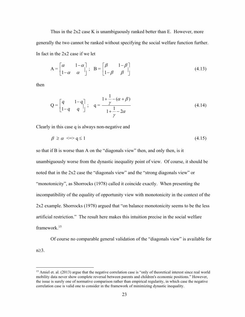
Thus in the 2x2 case K is unambiguously ranked better than E. However, more

generally the two cannot be ranked without specifying the social welfare function further.

In fact in the 2x2 case if we let

A = 1

1

; B = 1

1

(4.13)

then

Q = 1

1

q q

q q

; q =

11 ( )

11 2

(4.14)

Clearly in this case q is always non-negative and

<=> q 1 (4.15)

so that if B is worse than A on the “diagonals view” then, and only then, is it

unambiguously worse from the dynastic inequality point of view. Of course, it should be

noted that in the 2x2 case the “diagonals view” and the “strong diagonals view” or

“monotonicity”, as Shorrocks (1978) called it coincide exactly. When presenting the

incompatibility of the equality of opportunity view with monotonicity in the context of the

2x2 example. Shorrocks (1978) argued that “on balance monotonicity seems to be the less

artificial restriction.” The result here makes this intuition precise in the social welfare

framework.15

Of course no comparable general validation of the “diagonals view” is available for

n3.

15 Amiel et. al. (2013) argue that the negative correlation case is “only of theoretical interest since real world mobility data never show complete reversal between parents and children's economic positions.” However, the issue is surely one of normative comparison rather than empirical regularity, in which case the negative correlation case is valid one to consider in the framework of minimizing dynastic inequality.

24

A counter example is easily presented using the result comparing K and E for n=4.

0 0 0 1 ¼ ¼ ¼ ¼ K = 0 0 1 0 ; E = ¼ ¼ ¼ ¼ (4.16) 0 1 0 0 ¼ ¼ ¼ ¼ 1 0 0 0 ¼ ¼ ¼ ¼

On the diagonals view K is superior to E for n=4. But we already know from (4.12) that an

unambiguous raking on social welfare grounds is not available. More generally, for any

two bistochastic matrices A and B, let

D = B – A (4.17)

if B and A stand in the relation (4.1), then

dij = 1

[ ij – qij] +

1

n

ia jq – aij (4.18)

In particular,

dii = 1

ia iq + (1

- aii) (1 – qii) (4.19)

0

Thus any two matrices which stand in the relation (4.1) satisfy the diagonals view. But the

converse is not true: any two matrices which satisfy the diagonals view need not

necessarily stand in the relation (4.1) to each other – the counter example in (4.16)

establishes that.

A general interpretation of (4.1) can be provided by writing it as

B = [1

I] [I-Q] + AQ.

B can thus be seen as a matrix weighed sum of 1

I and A, the weights being Q and [I-Q].

If there exists a Q such that B can be written as this weighted sum, in a general sense B is

25

closer to the Identity matrix than A. If interpreted in this wide sense, the “diagonals view”

has a rationale in a social welfare function that is egalitarian with respect to dynastic

prospects.

For a specific application, consider the matrices A, B and C given below, which are

taken from Atkinson (1981a).

A = 0.48 0.42 0.10 0.00 0.25 0.34 0.27 0.14 0.19 0.17 0.37 0.27 0.08 0.07 0.26 0.59 B = 0.35 0.24 0.27 0.14 0.26 0.30 0.27 0.17 0.19 0.17 0.37 0.27 0.20 0.29 0.09 0.42 C = 0.44 0.23 0.19 0.14 0.32 0.26 0.25 0.17 0.18 0.36 0.27 0.19 0.06 0.15 0.29 0.50 Matrix C is a father to son, quartile to quartile, transition matrix for hourly earnings in

Britain, derived from the work of Atkinson, Maynard and Trinder (1983). Matrices A and

B are alternative specifications of father to son occupational transition matrices which are

got by adjusting the Goldthorpe (1980) data from its seven classes into four and enforcing

bistochasticity. Atkinson (1981a) provides a fuller discussion of the procedure, but

essentially matrix A has been derived by shifting weight towards the diagonal and matrix B

by shifting weight away from the diagonal. Atkinson compares C with A and C with B

using his criterion (2.11), and finds that C and A cannot be so ranked, but that “the earnings

transition matrix is welfare inferior to case B of the occupational status matrix.”

Can the same be said of the matrices using our criterion? For = 0.5 (an

intergenerational interest rate of 100%), we get the following Q matrices:

26

QCA = [I - C]-1 [I - A]

= 0.978 - 0.111 0.051 0.082 0.035 0.953 - 0.009 0.021 - 0.002 0.095 0.947 - 0.040 - 0.011 0.063 0.011 0.938

QBC = [I - B]-1 [I - C]

= 0.948 - 0.001 0.049 0.003 - 0.034 1.016 0.016 0.002 0.009 - 0.101 1.050 0.042 0.076 0.086 - 0.115 0.953

As in the case of Atkinson’s criterion, C cannot be ranked as better than A. However, what

is interesting is that B cannot be ranked as better than C, in contrast to the Atkinson

finding. Thus while it should be clear that there are a number of empirical problems in

comparing earnings transition matrices with occupational ones, our calculations

nevertheless indicate that a stress on dynastic inequality could alter rankings which

emphasize intertemporal non-separability.

27

5. Conclusion

The normative riposte to concerns about sharply rising inequality of income and

wealth, that it is intergenerational mobility and equality of opportunity which really matter,

need to be assessed with respect to specific social welfare functions which make explicit

the value judgments underlying the claim. An earlier literature, starting with the work of

Shorrocks (1978), Atkinson (1981a and 1981b), Atkinson and Bourguignon (1982)

attempted to do just this, and developed criteria for assessment of alternative patterns of

intergenerational mobility. Our contribution is in this vein, focusing on the implications of

intergenerational mobility for inequality among infinitely lived dynasties.

Restricting attention to bistochastic transition matrices in order to hold constant the

steady state snapshot income distribution, we have developed an explicit partial ordering

which ranks matrices on the criterion of dynastic inequality. A general interpretation of our

result is that when comparing two matrices, if one matrix is “further away” from the

identity matrix then it will lead to lower dynastic inequality. More specifically, the result

presents a computational procedure to check if one matrix dominates another on dynastic

inequality. We can also assess “equality of opportunity”, defined as identical prospects

irrespective of starting position, or identical rows of a transition matrix. We find that this is

not necessarily the mobility pattern which minimizes dynastic inequality, which requires

instead a degree of negative correlation between intergenerational outcomes.

Much remains to be done. At the theoretical level, we can sharpen our ordering by

restricting the class of transition matrices, for example to those which satisfy stochastic

monotonicity as suggested by Dardanoni, Fiorini and Forcini (2010). The criterion we have

developed can be applied to intergenerational transition matrices which are now being

28

estimated with newly available data. The earlier literature on normative measurement of

mobility needs to be revisited and extended to address the revived concerns on inequality

and mobility. Most importantly, the normative implications of the current inequality of

income for intergenerational inequality need to be assessed again with respect to alternative

sets of social welfare value judgments, perhaps bolstered by empirical investigation of

peoples’ views on mobility and inequality in its different dimensions, as developed by

Amiel et. al. (2013). Specifically, if “equality of opportunity” as captured identical rows of

a transition matrix (independence of future prospects from current income or wealth), does

indeed have normative significance as the best transition matrix, how do we reconcile this

with the outcome that it does not necessarily minimize dynastic inequality?

29

References

Aaberge, R., M. Mogstad and V. Peragine (2011): Measuring Long-Term Inequality of Opportunity,” Journal of Public Economics, Volume 95, Number 3, pp. 193-204.

Amiel, Yoram, Michele Bernasconi, Frank Cowell and Valentino Dardanoni (2013): “Do

We Value Mobility?” London School of Economics STCERD Discussion Paper, Number PEP 17, http://sticerd.lse.ac.uk/dps/pep/pep17.pdf

Arneson, Richard (2014): “Four Conceptions of Equal Opportunity,”

http://bfi.uchicago.edu/sites/default/files/research/Arneson.pdf Atkinson, A.B. (1981a): “On intergenerational income mobility in Britain,” Journal of Post

Keynesian Economics, Volume 3, pp. 194-218.

Atkinson, A.B. (1981b): “The Measurement of Economic Mobility” in Inkomensverdeling en openbare financien – Essays in Honour of Jan Pen (eds. - P J Eigjelshoven and L.J. van Gemerden), Het Spectrum, Utrecht, 9-24. Also published in Social Justice and Public Policy (ed. – A.B. Atkinson), Wheatsheaf Books Ltd, 1983, pp. 61-75.

Atkinson, A.B. and F. Bourguignon (1982): “The comparison of multi-dimensional

distributions of economic status,” Review of Economic Studies, Volume 49, pp, 183-201. Also published in Social Justice and Public Policy (ed. – A.B. Atkinson), Wheatsheaf Books Ltd, 1983, pp. 37-59.

Atkinson, A.B., A.K. Maynard and C.G. Trinder (1983): “Parents and children: incomes

in two generations,” London: Heinemann Educational Books. Chakravarty, S.R., B. Dutta and J.A. Weymark (1985): “Ethical indices of income

mobility,” Social Choice and Welfare, Volume 2, pp. 1-21. Corak, Miles (2013): “Income Inequality, Equality of Opportunity and Intergenerational

Mobility,” Journal of Economic Perspectives, Volume 27, Number 3, Summer 2013, pp. 79-102.

Dardanoni, V. (1993). Measuring social mobility. Journal of Economic Theory, Volume

61, pp. 372-394. Dardanoni, Valentino, Mario Fiorini and Antonio Forcina (2010). “Stochastic

Monotonicity in Intergenerational Mobility Tables.” Journal of Applied Econometrics, Vol. 27, No. 1, pp 85-107.

Dasgupta, P., A.K. Sen and D. Starrett (1973): “Notes on the measurement of inequality,”

Journal of Economic Theory. Volume 6, Number 2, pp. 180-187.

30

Dworkin, Ronald (1981): “What is Equality? Part 2: Equality of Resources” Philosophy and Public Affairs, Volume 10, No. 4, pp. 283-345.

Fields, G. S. & Ok, E. A. (1999). “The measurement of income mobility: An introduction

to the literature,” In J. Silber (Ed.) Handbook on income inequality measurement (pp. 557-596). Norwell, MA: Kluwer Academic Publishers.

Friedman, M. (1962): “Capitalism and freedom,” University of Chicago Press. Goldthorpe, J.H. (1980): “Social mobility and class structure in modern Britain,” London:

Oxford University Press. Kanbur, Ravi and V. Mukerji (1980): “Probabilistic equity and equality of opportunity in a

stochastic framework,” Arthaniti, Volume XX, pp. 1-9. Kanbur, Ravi and J.E. Stiglitz (1982): “Mobility and Inequality: a Utilitarian analysis,”

Economic Theory Discussion Paper No. 57, Department of Applied Economics, University of Cambridge.

Kanbur, Ravi and J.E. Stiglitz (1986): “Intergenerational Mobility and Dynastic

Inequality,” Woodrow Wilson School Discussion Paper in Economics, Number 111, Princeton University.

Kanbur, Ravi and J.O. Stromberg (1988): “Income Transitions and Income Distribution

Dominance,” Journal of Economic Theory, Volume 45, No. 2, pp. 408-417. Kanbur, Ravi and Adam Wagstaff (2014): “How Useful is Inequality of Opportunity as a

Policy Construct?” World Bank Policy Research Working Paper, Number 6980, http://www-wds.worldbank.org/external/default/WDSContentServer/WDSP/IB/2014/07/28/000158349_20140728112400/Rendered/PDF/WPS6980.pdf

Markandya, A. (1984): “The welfare measurement of changes in economic mobility,”

Economica. Volume 51, pp. 457-71. Piketty, Thomas (2014): Capital In the Twenty-First Century. Harvard University Press. Roemer, John E. (1998): Equality of Opportunity. Harvard University Press. Roemer, John E. (2004): “Equal Opportunity and Intergenerational Mobility: Going

Beyond Intergenerational Income Transition Matrices.” Chap. 3 in Generational Income Mobility in North America and Europe, edited by Miles Corak. Cambridge University Press.

Shorrocks, A.F. (1978): “The Measurement of mobility,” Econometrica, Volume 46, No.

5, pp. 1013-1024.

31

Stigltiz, Joseph, E. 2013. The Price of Inequality: How Today’s Divided Society Endangers Our Future. W.W. Norton and Company.

Stokey, N. (1998): “Shirtsleeves to Shirtsleeves: The Economics of Social Mobility,” in N.

L. Schwartz, D. Jacobs and E. Kalai (eds.) Frontiers of Research in Economic Theory: The Nancy L. Schwartz Memorial Lectures 1983-1997, pp. 210-241. Cambridge: Econometric Society Monographs.