Introduction to Graphical Models

Kai Yu

Google Whiteboard

2

"Google uses Bayesian filtering the way Microsoft uses the if statement”,

-- Joel Spolsky said to Peter Norvig

3

Graphical models: outline

§ What are graphical models? §  Inference §  Structure learning

Graphical models

§  A compact way to represent joint distributions

§  Useful to query various conditional probabilities

§  A powerful language to model real-world systems

§  Easy to plug in prior knowledge.

§  Extremely widely used!

8/9/12 4

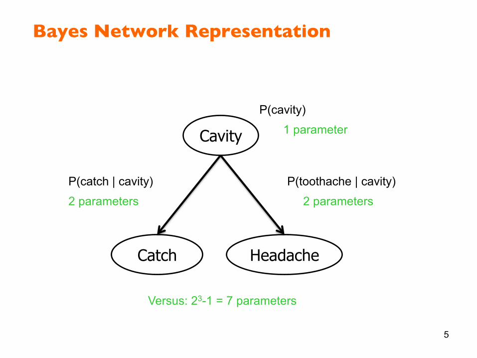
Bayes Network Representation

5

Cavity

Catch Headache

P(cavity)

P(catch | cavity) P(toothache | cavity)

1 parameter

2 parameters 2 parameters

Versus: 23-1 = 7 parameters

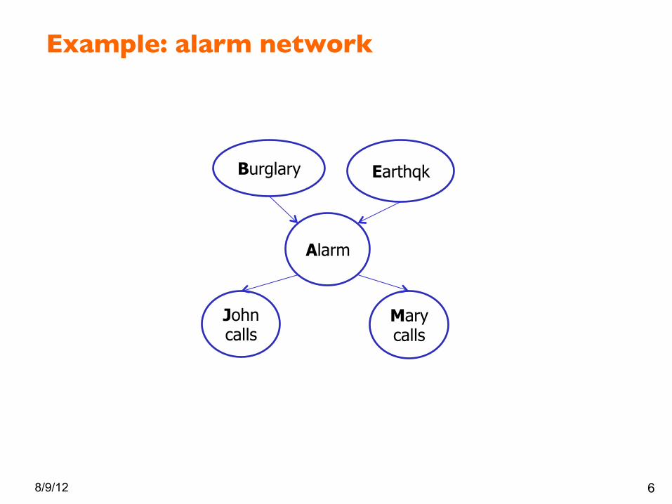
Example: alarm network

8/9/12 6

Burglary Earthqk

Alarm

John calls

Mary calls

A More Realistic Bayes Network

7

Example Bayes Network: Car

8

You may have seen this …

8/9/12 9

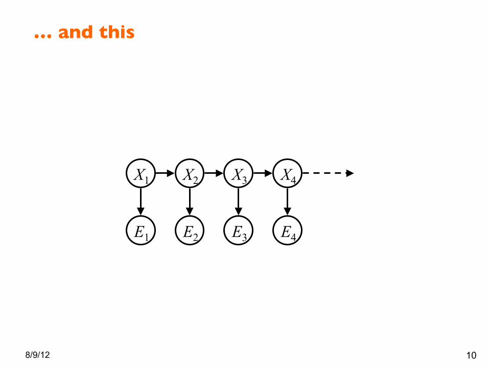
… and this

8/9/12 10

X5 X2

E1

X1 X3 X4

E2 E3 E4 E5

Graphical model notation

11

§  Nodes: variables (with domains) –  Can be assigned (observed) or unassigned

(unobserved)

§  Arcs: interactions –  Indicate “direct influence” between variables –  Formally: encode conditional independence

(more later)

§  For now: imagine that arrows mean direct causation (they may not!)

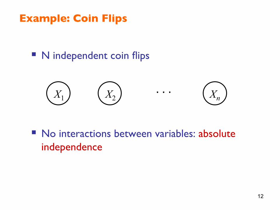
Example: Coin Flips

X1 X2 Xn

§  N independent coin flips

§  No interactions between variables: absolute independence

12

Example: Alarm Network

§  Variables –  B: Burglary

–  A: Alarm goes off –  M: Mary calls

–  J: John calls –  E: Earthquake!

13

Burglary Earthquake

Alarm

John calls

Mary calls

Probabilities in BNs

Bayes nets implicitly encode joint distributions

–  As a product of local conditional distributions –  To see what probability a BN gives to a full assignment,

multiply all the relevant conditionals together:

–  Example:

14

15

Family of Alarm

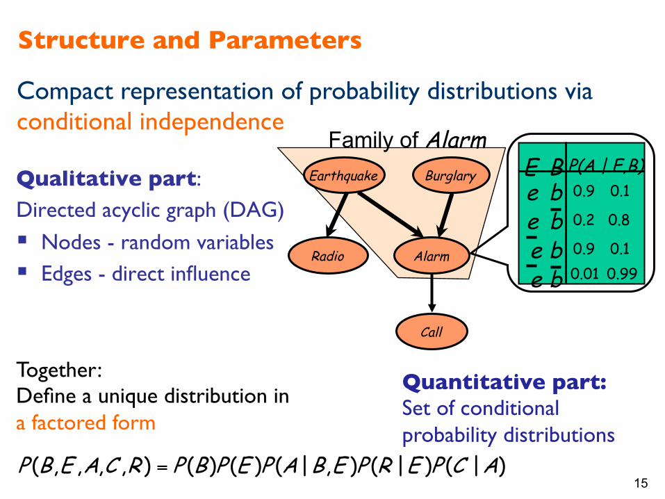
Structure and Parameters

Qualitative part: Directed acyclic graph (DAG)

§  Nodes - random variables §  Edges - direct influence

Quantitative part: ���Set of conditional probability distributions

0.9 0.1 e

b e

0.2 0.8

0.01 0.99 0.9 0.1

b e

b b

e

B E P(A | E,B) Earthquake

Radio

Burglary

Alarm

Call

Compact representation of probability distributions via conditional independence

Together: Define a unique distribution in a factored form

)|()|(),|()()(),,,,( ACPERPEBAPEPBPRCAEBP =

Example: Coin Flips

h 0.5 t 0.5

h 0.5 t 0.5

h 0.5 t 0.5

X1 X2 Xn

Only distributions whose variables are absolutely independent can be represented by a Bayes’ net with no arcs.

16

Example: Alarm Network

Burglary Earthqk

Alarm

John calls

Mary calls

B P(B)

+b 0.001

¬b 0.999

E P(E)

+e 0.002

¬e 0.998

B E A P(A|B,E)

+b +e +a 0.95

+b +e ¬a 0.05

+b ¬e +a 0.94

+b ¬e ¬a 0.06

¬b +e +a 0.29

¬b +e ¬a 0.71

¬b ¬e +a 0.001

¬b ¬e ¬a 0.999

A J P(J|A)

+a +j 0.9

+a ¬j 0.1

¬a +j 0.05

¬a ¬j 0.95

A M P(M|A)

+a +m 0.7

+a ¬m 0.3

¬a +m 0.01

¬a ¬m 0.99

18

Example: “ICU Alarm” network

Domain: Monitoring Intensive-Care Patients §  37 variables §  509 parameters

…instead of 237

PCWP CO

HRBP

HREKG HRSAT

ERRCAUTER HR HISTORY

CATECHOL

SAO2 EXPCO2

ARTCO2

VENTALV

VENTLUNG VENITUBE

DISCONNECT

MINVOLSET

VENTMACH KINKEDTUBE INTUBATION PULMEMBOLUS

PAP SHUNT

ANAPHYLAXIS

MINOVL

PVSAT

FIO2 PRESS

INSUFFANESTH TPR

LVFAILURE

ERRBLOWOUTPUT STROEVOLUME LVEDVOLUME

HYPOVOLEMIA

CVP

BP

Causal Chains

§  This configuration is a “causal chain”

–  Is X independent of Z given Y?

–  Evidence along the chain “blocks” the influence

X Y Z

Yes!

X: Low pressure

Y: Rain

Z: Traffic

19

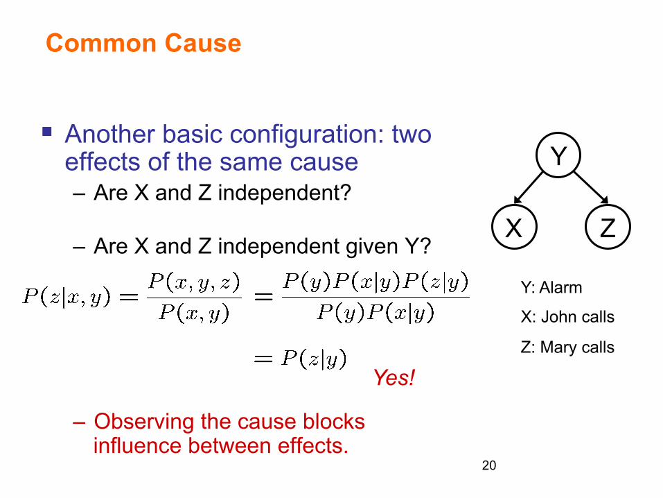
Common Cause

§  Another basic configuration: two effects of the same cause –  Are X and Z independent?

–  Are X and Z independent given Y?

–  Observing the cause blocks influence between effects.

X

Y

Z

Yes!

Y: Alarm

X: John calls

Z: Mary calls

20

Common Effect

§  Last configuration: two causes of one effect (v-structures) –  Are X and Z independent?

•  Yes: the ballgame and the rain cause traffic, but they are not correlated

•  Still need to prove they must be (try it!)

–  Are X and Z independent given Y? •  No: seeing traffic puts the rain and the

ballgame in competition as explanation?

–  This is backwards from the other cases •  Observing an effect activates influence

between possible causes.

X

Y

Z

X: Raining

Z: Ballgame

Y: Traffic

21

The General Case

§  Any complex example can be analyzed using these three canonical cases

§  General question: in a given BN, are two variables independent (given evidence)?

§  Solution: analyze the graph

22

Reachability (D-Separation)

§  Question: Are X and Y conditionally independent given evidence vars {Z}? –  Yes, if X and Y “separated” by Z –  Look for active paths from X to Y

–  No active paths = independence!

§  A path is active if each triple is active: –  Causal chain A → B → C where B

is unobserved (either direction) –  Common cause A ← B → C

where B is unobserved –  Common effect (aka v-structure)

A → B ← C where B or one of its descendents is observed

§  All it takes to block a path is a single inactive segment

Active Triples Inactive Triples

Let’s analyze this case

Burglary Earthquake

Alarm

John calls

Mary calls

Modeling, Inference, and Learning

§  A Bayes net is an efficient encoding of a probabilistic model of a domain

§  Questions we can ask: – Modeling: what BN is most appropriate for a given domain? –  Inference: given a fixed BN, what is P(X | e)? –  Learning: given data, how to obtain a BN (structure&para.)?

25

26

Simple probabilistic model:���linear regression

Y

X

Y = µ + β X + noise

27

Simple probabilistic model:���linear regression

Y

Y = µ + β X + noise

X

“Learning” = estimating parameters µ, β, σ from (x,y) pairs.

28

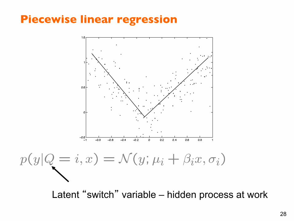
Piecewise linear regression

Latent “switch” variable – hidden process at work

29

Probabilistic graphical model for ���piecewise linear regression

X

Y

Q

• Hidden variable Q chooses which set of���parameters to use for predicting Y.

• Value of Q depends on value of input X.

output

input

• This is an example of “mixtures of experts”

Learning is harder because Q is hidden, so we don’t know which data points to assign to each line; can be solved with EM

30

Family of graphical models

Probabilistic models Graphical models

Directed Undirected

Bayes nets MRFs

DBNs

Hidden Markov Model (HMM)

Naïve Bayes classifier

Mixtures of experts

Kalman filter model Ising model

31

Success stories for graphical models

§  Multiple sequence alignment §  Forensic analysis §  Medical and fault diagnosis

§  Speech recognition §  Image understanding §  Visual tracking

§  Channel coding at Shannon limit §  Genetic pedigree analysis § …

32

Graphical models: outline

§ What are graphical models? §  Inference §  Structure learning

33

Probabilistic Inference

§ Posterior probabilities –  Probability of any event given any evidence

§ P(X|E)

Earthquake

Radio

Burglary

Alarm

Call

Radio

Call

34

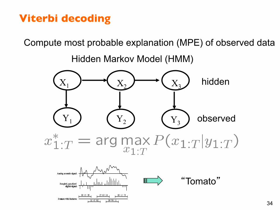
Viterbi decoding

Y1 Y3

X1 X2 X3

Y2

Compute most probable explanation (MPE) of observed data

Hidden Markov Model (HMM)

“Tomato”

hidden

observed

35

Inference: computational issues

PCWP CO HRBP

HREKG HRSAT

ERRCAUTER HR HISTORY

CATECHOL

SAO2 EXPCO2

ARTCO2

VENTALV

VENTLUNG VENITUBE

DISCONNECT

MINVOLSET

VENTMACH KINKEDTUBE INTUBATION PULMEMBOLUS

PAP SHUNT

MINOVL

PVSAT

PRESS

INSUFFANESTH TPR

LVFAILURE

ERRBLOWOUTPUT STROEVOLUME LVEDVOLUME

HYPOVOLEMIA

CVP

BP

Easy Hard

Chains

Trees

Grids

Dense, loopy graphs

36

Inference: computational issues

PCWP CO HRBP

HREKG HRSAT

ERRCAUTER HR HISTORY

CATECHOL

SAO2 EXPCO2

ARTCO2

VENTALV

VENTLUNG VENITUBE

DISCONNECT

MINVOLSET

VENTMACH KINKEDTUBE INTUBATION PULMEMBOLUS

PAP SHUNT

MINOVL

PVSAT

PRESS

INSUFFANESTH TPR

LVFAILURE

ERRBLOWOUTPUT STROEVOLUME LVEDVOLUME

HYPOVOLEMIA

CVP

BP

Easy Hard

Chains

Trees

Grids

Dense, loopy graphs

Many difference inference algorithms, both exact and approximate

37

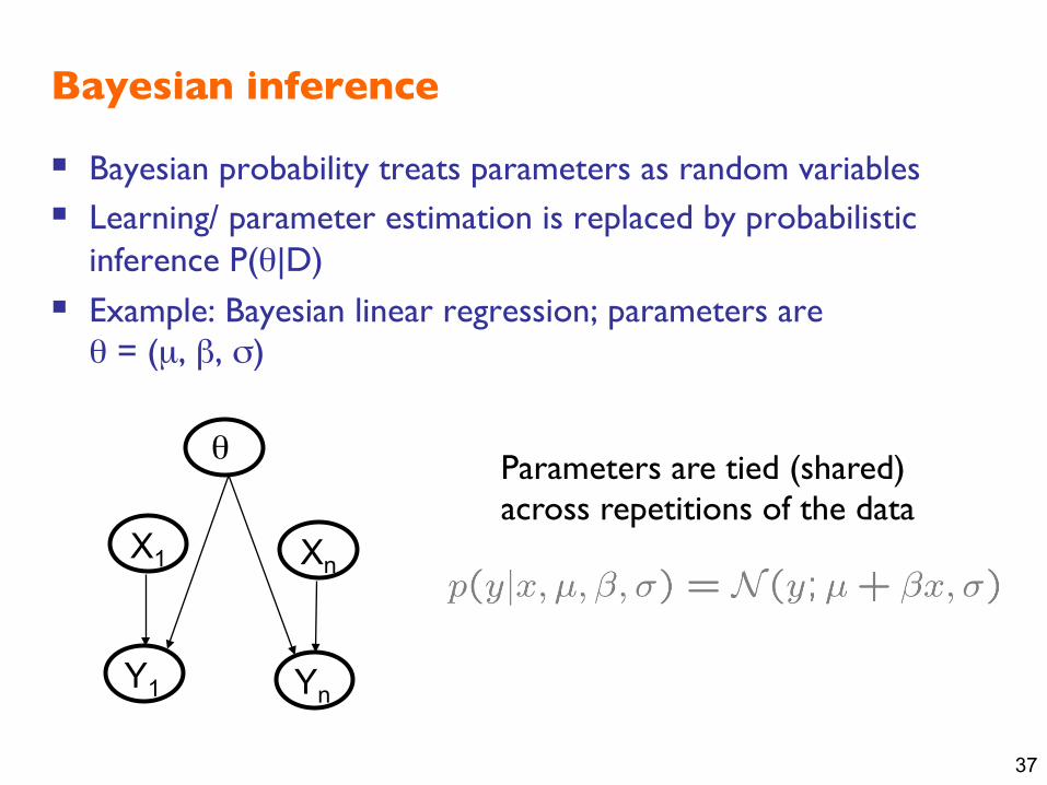
Bayesian inference

§  Bayesian probability treats parameters as random variables §  Learning/ parameter estimation is replaced by probabilistic

inference P(θ|D)

§  Example: Bayesian linear regression; parameters are���θ = (µ, β, σ)

θ

X1

Y1

Xn

Yn

Parameters are tied (shared) ���across repetitions of the data

38

Bayesian inference

§  + Elegant – no distinction between parameters and other hidden variables

§  + Can use priors to learn from small data sets (c.f., one-shot learning by humans)

§  - Math can get hairy

§  - Often computationally intractable (hence variational, MCMC …)

39

Graphical models: outline

§ What are graphical models? §  Inference §  Structure learning

40

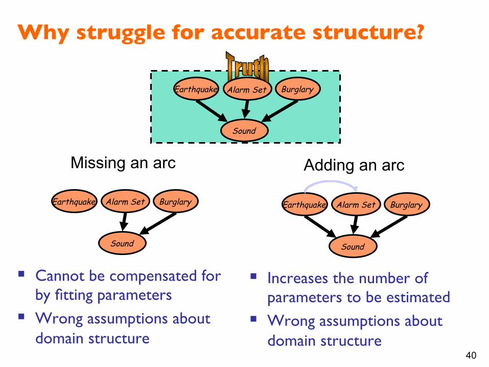
Why struggle for accurate structure?

§  Increases the number of parameters to be estimated

§  Wrong assumptions about domain structure

§  Cannot be compensated for by fitting parameters

§  Wrong assumptions about domain structure

Earthquake Alarm Set

Sound

Burglary Earthquake Alarm Set

Sound

Burglary

Earthquake Alarm Set

Sound

Burglary

Adding an arc Missing an arc

41

Score­based Learning

E, B, A <Y,N,N> <Y,Y,Y> <N,N,Y> <N,Y,Y> . . <N,Y,Y>

E B

A

E

B

A E

B A

Search for a structure that maximizes the score

Define scoring function that evaluates how well a structure matches the data

42

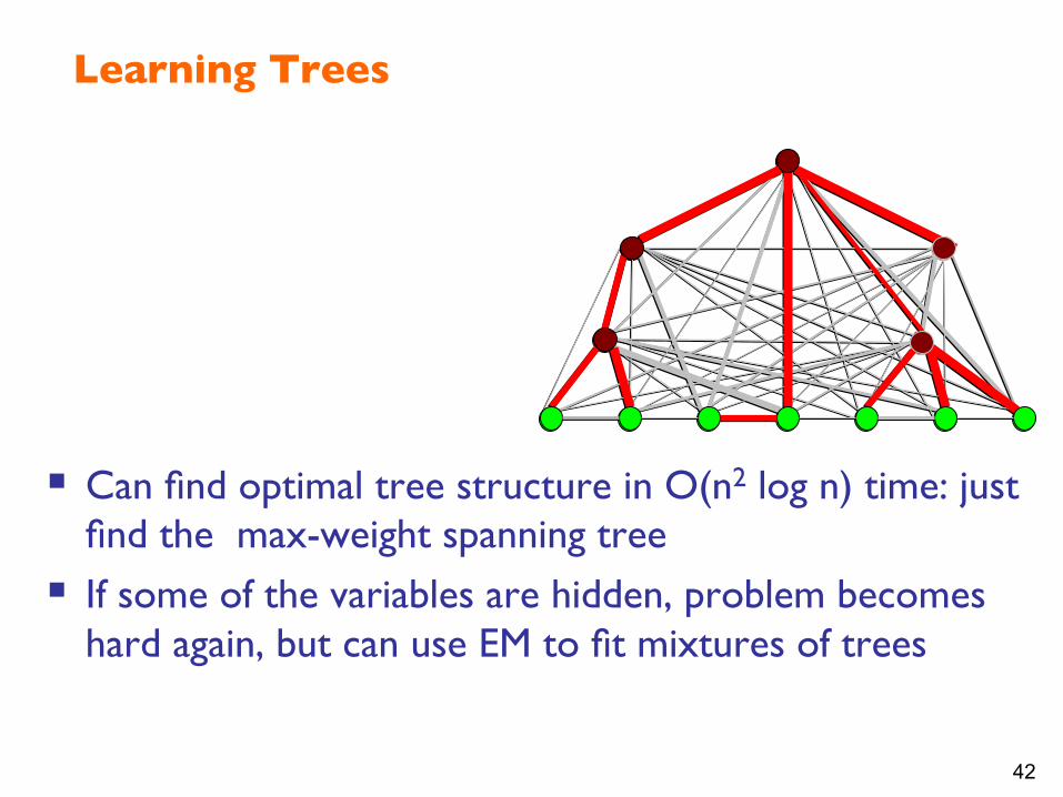
Learning Trees

§  Can find optimal tree structure in O(n2 log n) time: just find the max-weight spanning tree

§  If some of the variables are hidden, problem becomes hard again, but can use EM to fit mixtures of trees

43

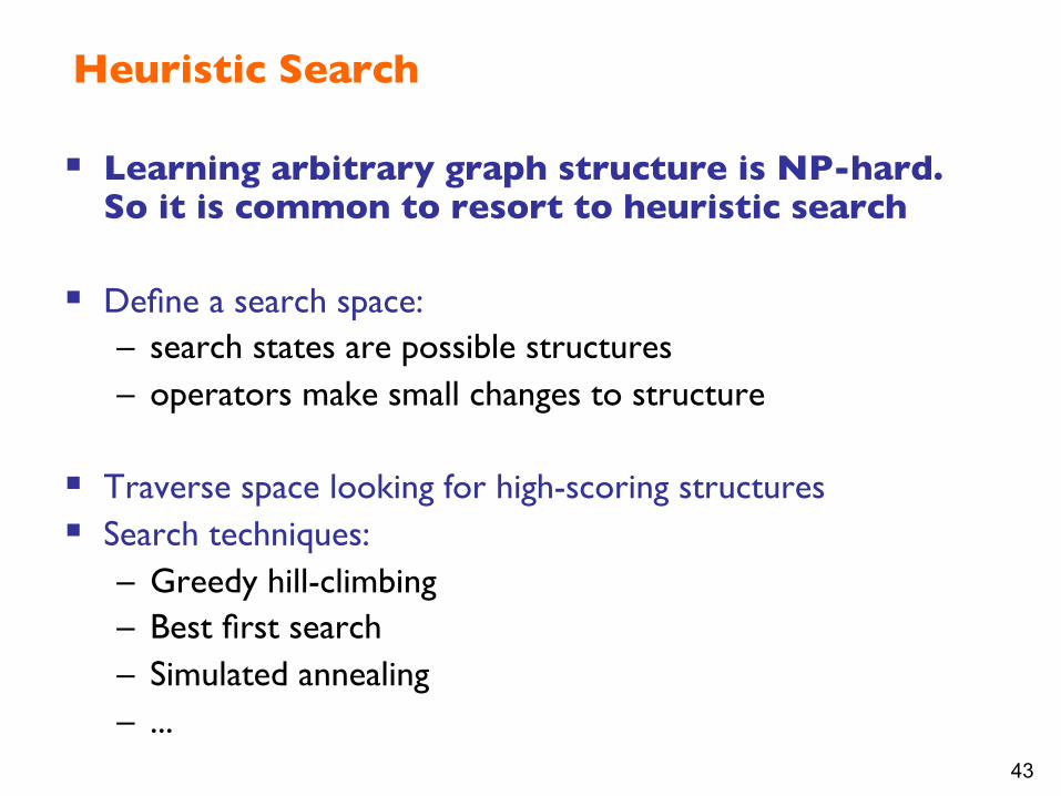
Heuristic Search §  Learning arbitrary graph structure is NP-hard.���

So it is common to resort to heuristic search

§  Define a search space: –  search states are possible structures –  operators make small changes to structure

§  Traverse space looking for high-scoring structures §  Search techniques:

–  Greedy hill-climbing –  Best first search –  Simulated annealing –  ...

44

Local Search Operations

§  Typical operations:

S C

E

D

Add C →D

S C

E

D

S C

E

D

S C

E

D

Δscore = S({C,E} →D) - S({E} →D)

45

Problems with local search S(

G|D

)

Easy to get stuck in local optima

“truth”

you

46

Problems with local search II

E

R

B

A

C

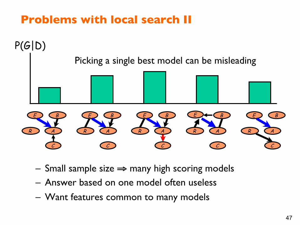
P(G|D) Picking a single best model can be misleading

47

Problems with local search II

–  Small sample size ⇒ many high scoring models –  Answer based on one model often useless

–  Want features common to many models

E

R

B

A

C

E

R

B

A

C

E

R

B

A

C

E

R

B

A

C

E

R

B

A

C

P(G|D) Picking a single best model can be misleading

48

Bayesian Approach to Structure Learning

§  Posterior distribution over structures §  Estimate probability of features

–  Edge X→Y –  Path X→… → Y –  …

∑=G

DGPGfDfP )|()()|(Feature of G, e.g., X→Y Indicator function

for feature f

Bayesian score for G

49

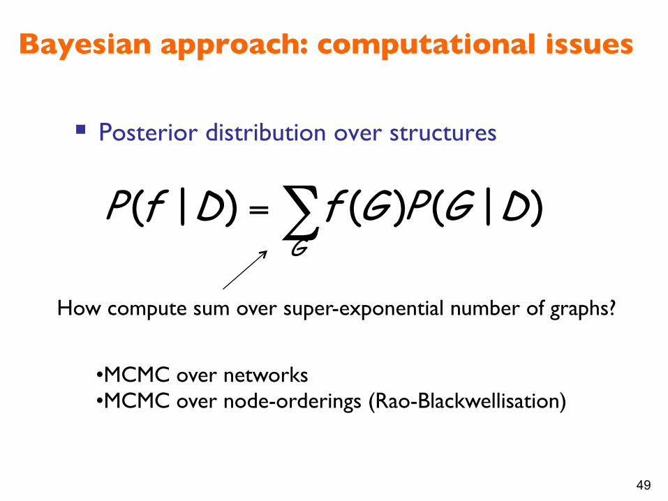
Bayesian approach: computational issues

§  Posterior distribution over structures

∑=G

DGPGfDfP )|()()|(

How compute sum over super-exponential number of graphs?

• MCMC over networks • MCMC over node-orderings (Rao-Blackwellisation)

50

Structure learning: Phylogenetic Tree Reconstruction (Friedman et al.)

Input: Biological sequences Human CGTTGC…

Chimp CCTAGG…

Orang CGAACG… ….

Output: a phylogeny

leaf

10 billion years

Uses structural EM, with max-spanning-tree���in the inner loop

51

Structure learning: other issues

§  Discovering latent variables §  Learning causal models §  Learning from relational data

52

Discovering latent variables

a) 17 parameters b) 59 parameters

There are some techniques for automatically detecting the���possible presence of latent variables

53

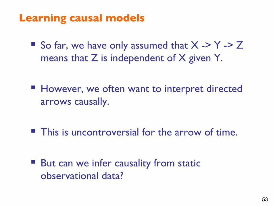
Learning causal models

§  So far, we have only assumed that X -> Y -> Z means that Z is independent of X given Y.

§  However, we often want to interpret directed arrows causally.

§  This is uncontroversial for the arrow of time.

§  But can we infer causality from static observational data?

54

Learning causal models

§ We can infer causality from static observational data if we have at least four measured variables and certain “tetrad” conditions hold.

§  See books by Pearl et al. §  However, we can only learn up to Markov equivalence,

not matter how much data we have.

X Y Z

X Y Z

X Y Z

X Y Z

Causality?

§  When Bayes’ nets reflect the true causal patterns: –  Often simpler (nodes have fewer parents) –  Often easier to think about –  Often easier to elicit from experts

§  BNs need not actually be causal –  Sometimes no causal net exists over the domain –  End up with arrows that reflect correlation, not causation

§  What do the arrows really mean? –  Topology may happen to encode causal structure –  Topology only guaranteed to encode conditional

independence

55

56

Learning from relational data

Can we learn concepts from a set of relations between objects, instead of/in addition to just their attributes? Example: user-movie preference data

57

Learning from relational data: approaches

§  Probabilistic relational models (PRMs) –  Reify a relationship (arcs) between nodes (objects)

by making into a node (hypergraph)

§  Inductive Logic Programming (ILP) –  Top-down, e.g., FOIL (generalization of C4.5)

–  Bottom up, e.g., PROGOL (inverse deduction)

58

Summary: ���a “graphical model” of graphical models A Generative Model for Generative Models

Gaussian

Factor Analysis (PCA)

Mixture of Factor Analyzers

Mixture of Gaussians

(VQ)

Cooperative Vector

Quantization

SBN, Boltzmann Machines

Factorial HMM

HMM

Mixture of

HMMs

Switching State-space

Models

ICALinear

Dynamical Systems (SSMs)

Mixture of LDSs

Nonlinear Dynamical Systems

Nonlinear Gaussian

Belief Nets

mix

mix

mix

switch

red-dim

red-dim

dyn

dyn

dyn

dyn

dyn

mix

distrib

hier

nonlinhier

nonlin

distrib

mix : mixture red-dim : reduced dimension dyn : dynamics distrib : distributed representation hier : hierarchical nonlin : nonlinear switch : switching