MAN/HEP/2014/13, TUM-HEP-962-14

October 2014

Kadanoff–Baym Approach to Flavour Mixingand Oscillations in Resonant Leptogenesis

P. S. Bhupal Deva, Peter Millingtonb, Apostolos Pilaftsisa, Daniele Teresia

aConsortium for Fundamental Physics, School of Physics and Astronomy,University of Manchester, Manchester M13 9PL, United Kingdom.

bPhysik Department T70, James-Franck-Straße,Technische Universitat Munchen, 85748 Garching, Germany.

Abstract

We describe a loopwise perturbative truncation scheme for quantum transport equa-tions in the Kadanoff–Baym formalism, which does not necessitate the use of the so-calledKadanoff–Baym or quasi-particle ansaetze for dressed propagators. This truncation schemeis used to study flavour effects in the context of Resonant Leptogenesis (RL), showing ex-plicitly that, in the weakly-resonant regime, there exist two distinct and pertinent flavoureffects in the heavy-neutrino sector: (i) the resonant mixing and (ii) the oscillations be-tween different heavy-neutrino flavours. Moreover, we illustrate that Kadanoff–Baym andquasi-particle ansaetze, whilst appropriate for the flavour-singlet dressed charged-lepton andHiggs propagators of the RL scenario, should not be applied to the dressed heavy-neutrinopropagators. The use of these approximations for the latter is shown to capture only flavouroscillations, whilst discarding the separate phenomenon of flavour mixing.

Keywords: Non-equilibrium thermal field theory, Kadanoff–Baym equations, Resonant Leptogenesis.arX

iv:1

410.

6434

v2 [

hep-

ph]

15

Dec

201

4

Contents

1 Introduction 2

2 Flavour-Covariant Scalar Model of RL 4

3 Quantum Transport Equations 9

4 Flavour Mixing and Kadanoff–Baym Ansaetze 15

5 Approximate Analytic Solution for the Lepton Asymmetry 19

6 Conclusions 22

Appendix A Resummed Thermal Propagators and Yukawa Couplings 23

1. Introduction

The scenario of leptogenesis [1] can be regarded as a cosmological consequence of theseesaw mechanism [2–6], thereby providing an elegant unifying framework to account forboth the observed baryon asymmetry of our Universe (BAU) and the smallness of thelight-neutrino masses [7]. The key ingredients are heavy Majorana neutrinos, whose out-of-equilibrium decays provide an initial excess in lepton number (L). This excess is subse-quently converted to a net baryon number (B) via the equilibrated (B + L)-violating inter-actions of the electroweak sphalerons [8]. The L-violating Majorana mass terms, complexYukawa couplings and expansion of the Universe fulfill the necessary Sakharov conditions [9]for dynamically generating the BAU, namely B, C and CP violation, together with out-of-equilibrium dynamics. For a review on various aspects of leptogenesis, see e.g. [10] andreferences therein.

An attractive possibility of testing leptogenesis in foreseeable laboratory experiments isprovided by the mechanism of Resonant Leptogenesis (RL) [11–13]. This relies on the factthat the heavy Majorana neutrino self-energy effects on the leptonic CP -asymmetry (the ε-type effects) become dominant [14–16] and get resonantly enhanced, when at least two of theheavy neutrinos have a small mass difference comparable to their decay widths [11, 12]. Theresonant enhancement of the CP -asymmetry enables a successful low-scale leptogenesis [13,17], whilst retaining perfect agreement with the active neutrino oscillation data [7]. Thislevel of testability is further improved in the scenario of Resonant `-Genesis (RL`), wherethe final lepton asymmetry is dominantly generated and stored in a single lepton flavour` [18, 19]. In such models, the heavy neutrinos could be at a scale as low as the electroweakscale [17], whilst still having sizable couplings to other charged-lepton flavours `′ 6= `. Thus,RL` scenarios may be testable in the run-II phase of the LHC [20–25] as well as in variouslow-energy experiments searching for lepton flavour/number violation [17, 19, 26, 27].

2

In RL models, with quasi-degenerate heavy Majorana neutrinos, flavour effects in bothheavy-neutrino [12, 17–19, 28–33] and charged-lepton [34–41] sectors, as well as the inter-play between them, can play an important role in determining the final lepton asymmetry.These intrinsically-quantum effects can be accounted for by extending the classical flavour-diagonal Boltzmann equations for the number densities of individual flavour species to asemi-classical evolution equation for a matrix of number densities, analogous to the for-malism presented in [42] for light neutrinos. This approach, the so-called ‘density matrix’formalism, has been adopted for various leptogenesis scenarios [31, 32, 37, 41, 43–48]. Aconsistent treatment of all pertinent flavour effects, including flavour mixing, oscillationsand off-diagonal (de)coherences, necessitates a fully flavour-covariant formalism, which wasrecently developed in [49] (for an executive summary, see [50]). This provides a complete andunified description of RL. Moreover, the resonant mixing of different heavy-neutrino flavoursand coherent oscillations between them were found to be two distinct physical phenomena,in analogy with the experimentally-distinguishable phenomena of mixing and oscillationsin the neutral K, D, B and Bs-meson systems [7] 1. In particular, we draw attention tothe phenomenon of oscillations via regeneration for the kaon system in medium [51, 52].A proper treatment of these flavour effects in this fully flavour-covariant formalism couldlead to a significant enhancement in the final lepton asymmetry, as compared to partiallyflavour-dependent or flavour-diagonal limits, as illustrated numerically in [49] within thecontext of an RLτ model.2

On the other hand, there has been significant progress in the literature, attempting to gobeyond the semi-classical ‘density matrix’ approach [42] to transport phenomena by means ofthe quantum field-theoretic analogues of the Boltzmann equations (see e.g. [57, 58]), knownas the Kadanoff–Baym (KB) equations [59] (for reviews, see [60–62]). This system of quan-tum Boltzmann equations is commonly derived from the Cornwall-Jackiw-Tomboulis (CJT)effective action [62–66] of the Schwinger-Keldysh [67, 68] closed-time path (CTP) formal-ism of non-equilibrium thermal field theory [69–71]. The KB equations are manifestly non-Markovian, describing the non-equilibrium time-evolution of two-point correlation functions,and have been studied extensively in various scenarios of leptogenesis [72–97]. In particu-lar, these ‘first-principles’ approaches to leptogenesis can, in principle, account consistentlyfor all off-shell, finite-width and flavour effects, including thermal corrections. However,the loopwise perturbative expansion of non-equilibrium propagators is normally spoiled bymathematical pathologies, known as pinch singularities [98–104], arising from ill-definedproducts of Dirac delta functions with identical arguments. Thus, in order to define andextract physically-meaningful quantities, such as particle number densities, one often resortsto particular approximations, specifically gradient expansion of time-derivatives in the so-called Wigner representation [105–109] and quasi-particle ansaetze [110–114] for the form of

1 This was also shown explicitly in the context of cascade decays of heavy particles, where the time-scalesfor mixing and oscillation are well separated [53–56].

2 Note that in RL` scenarios, the quantum (de)coherence effects in the charged-lepton sector must alsobe included, which might further contribute to the enhancement of the final lepton asymmetry, dependingupon the model parameters [49].

3

the dressed propagators.

Recently, a new perturbative formulation of non-equilibrium thermal field theory [115](for an overview, see [116]) was developed, which is free of the mathematically ill-definedpinch singularities previously thought to spoil such approaches. Within this framework, onemay define a perturbative loopwise truncation scheme for quantum transport equations thatis valid to all orders in a gradient expansion, whilst capturing non-Markovian dynamics,memory and threshold effects. As a result, physically-meaningful particle number densitiescan be derived directly from the Noether charge, without the need for quasi-particle ansaetze.

In this paper, we use the formalism of [115] to obtain a well-defined loopwise perturba-tive truncation scheme for the KB equations in the weakly-resonant regime of RL. This isachieved without resorting to a quasi-particle ansatz for the dressed heavy-neutrino propa-gator. We find that the source term for the lepton asymmetry obtained in this KB approachis exactly the same as that derived in [49] using a semi-classical Boltzmann approach. Thus,we prove that there is no double-counting of flavour effects captured in the fully flavour-covariant semi-classical formalism of [49]. Moreover, we confirm that flavour mixing andoscillations are two physically-distinct phenomena also in improved quantum Boltzmanntreatments, as is the case in the semi-classical approach. Finally, we show that the use ofKB or quasi-particle ansaetze for the resummed heavy-neutrino propagators captures onlyflavour oscillations and not the separate phenomenon of flavour mixing. As a result, theapplication of such approximations may lead to an underestimate of the generated leptonasymmetry by a factor of order two in the weakly-resonant regime.

The rest of the paper is organized as follows. In Section 2, we introduce a flavour-covariant scalar toy model of RL and describe its flavour-covariant canonical quantizationwithin the context of perturbative non-equilibrium thermal field theory. In Section 3, wederive the heavy-neutrino and charged-lepton quantum transport equations relevant to thesource term for the lepton asymmetry. Subsequently, in Section 4, we illustrate that the KBansaetze are not appropriate in the presence of particle mixing and that such approxima-tions, when applied to the resummed heavy-neutrino propagator, discard the phenomenonof flavour mixing. We then proceed to derive the form of the source term for the leptonasymmetry, incorporating both flavour mixing and oscillation. In Section 5, we derive anapproximate analytic solution for the lepton asymmetry, making comparison with existingresults. Finally, Section 6 summarizes our conclusions. Further technical details of the re-summation of the heavy-neutrino Yukawa couplings and thermal propagators are providedin Appendix A.

2. Flavour-Covariant Scalar Model of RL

In order to study the role of heavy-neutrino flavour effects in RL within the KB formalism,but without the technical complications arising from the fermionic nature of the heavyneutrinos and charged leptons, we consider a simple toy model of RL with two real scalarfields Nα (with α = 1, 2), one complex scalar field L and a real scalar Φ. This simple modelincludes all qualitatively important features of leptogenesis, where the two real scalar fields

4

mimic heavy Majorana neutrinos of two flavours and the complex scalar field models chargedleptons of a single flavour. Moreover, Φ plays the role of the the Standard Model (SM) Higgsfield. The approximate global U(1) symmetry associated with the complex scalar field Lcorresponds to the lepton number. Similar toy models have been used extensively to studyRL in the KB formalism [77, 78, 81, 93, 96, 108].

In order to capture fully the flavour-dynamics in the heavy-neutrino sector, we adopt theflavour-covariant formulation developed in [49]. Therein, the heavy-neutrino field transformsin the fundamental representation of U(NN), i.e. Nα → N ′α = U β

α Nβ, where U βα ∈ U(NN).3

The relevant part of the Lagrangian may then be written in the following manifestly-covariant form:

LN = hαL†ΦNα +1

4Nα[m2

N ]αβNβ + H.c. , (2.1)

where the tree-level Yukawa coupling parameters hα transform as a vector and the heavy-neutrino mass-squared matrix [m2

N ]αβ transforms as a rank-2 tensor of U(NN), i.e.

hα → h′α = Uαβ h

β , [m2N ]αβ → [m′2N ]αβ = Uα

γ Uβδ [m2

N ]γδ . (2.2)

The basic Sakharov conditions [9] for the generation of the BAU are satisfied in this toymodel as follows. The lepton number is explicitly broken by the L†ΦN term in (2.1). Also,the charge conjugation (C) symmetry is violated, provided that arg(h1) 6= arg(h2) and theheavy neutrinos are non-degenerate. In this model, C-violation will also imply CP -violation,since CP -transformations on the scalar fields are identical to C-transformations, up to a signchange of the spatial coordinates. Finally, the out-of-equilibrium condition can be satisfiedby the decays of Nα in an expanding Universe.

In order to define unambiguously the physical objects that enter into the heavy-neutrinorate equation, we follow the perturbative framework of non-equilibrium thermal field the-ory described in [115]. This novel approach differs from the standard interpretation ofthe Schwinger-Keldysh closed-time path (CTP) formalism in the time-dependence of freepropagators. Specifically, the free positive-frequency Wightman propagator of [115], in theinteraction picture, is defined as

[i∆N, 0> (x, y, tf ; ti)]

βα = 〈Nα(x; ti)N

β(y; ti)〉t ≡1

ZTr ρ(tf ; ti)Nα(x; ti)N

β(y; ti) , (2.3)

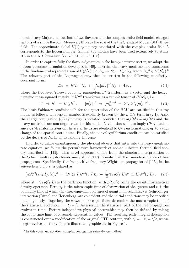
where Z = Tr ρ(tf ; ti) is the partition function, with ρ(tf ; ti) being the quantum-statisticaldensity operator. Here, tf is the microscopic time of observation of the system and ti is theboundary time at which the three equivalent pictures of quantum mechanics, viz. Schrodinger,interaction (Dirac) and Heisenberg, are coincident and the initial conditions may be specifiedunambiguously. Together, these two microscopic times determine the macroscopic time ofthe statistical evolution: t = tf − ti. As a result, the statistical part of the free propagatorsevolves in time. Picture-independent physical observables may then be defined by takingthe equal-time limit of ensemble expectation values. The resulting path-integral descriptionis constructed over a modification of the original CTP contour, with tf = − ti = t/2, whoselength evolves in time. This is illustrated graphically in Figure 1.

3 In this covariant notation, complex conjugation raises/lowers indices.

5

bb

b

Re t

Im t

ti = − t/2

tf − iǫ/2 = (t − iǫ)/2ti − iǫ = − t/2 − iǫ

C+

C−

macroscopic time t = tf − ti

initial conditions ρ(ti; ti)(macroscopic time t = 0)

observation〈•〉t = Z−1 Tr [ ρ(tf ; ti) • ]

Figure 1: The CTP contour C+ ∪ C− in the analytically-continued complex-time (t) plane,indicating the relationship between macroscopic and microscopic times t = tf − ti, as definedin the perturbative non-equilibrium formulation of thermal Quantum Field Theory in [115].

This is in stark contrast with earlier CTP constructions (see e.g. [70, 71]), which usethe Heisenberg picture and a contour of fixed length. In these earlier treatments, the freepropagator is given by

[i∆N, 0> (x, y, 0)] β

α = 〈Nα(x)Nβ(y)〉0 ≡1

ZTr ρ(0)Nα(x)Nβ(y) , (2.4)

whose role is to encode the initial conditions at a time t = 0.

With the recognition of the necessary dependence of diagrammatic series on the twomicroscopic times tf and ti, it was shown in [115] that one may arrive at a perturbativeframework of non-equilibrium field theory, using (2.3), that captures fully non-Markovianeffects and is free of the so-called pinch singularities [98–104], previously thought to spoilsuch perturbative approaches when constructed using (2.4). As a result, it is now possi-ble to obtain a well-defined perturbative loopwise truncation scheme for quantum transportequations, using the propagator (2.3) instead of (2.4). Moreover, it was illustrated that thisloopwise perturbative truncation was two-fold, proceeding (i) spectrally: the truncation ofthe external leg of the transport equation determines the order of spectral dressing of thespecies being counted and (ii) statistically: the truncation of the self-energies determines theset of processes driving the statistical evolution of the system. In this way, quantum trans-port equations are obtained without the need for quasi-particle approximations or gradientexpansion.

Within the union of these flavour-covariant and perturbative non-equilibrium frameworks[49, 115], the plane-wave decomposition of the heavy-neutrino field takes the following form:

Nα(x; ti) =

∫

k

[(2EN(k))−1/2

] β

α

([e−ik·x

] γ

βaγ(k, 0; ti) +

[e+ik·x] γ

βGγδ a

δ(k, 0; ti)), (2.5)

6

where∫k≡∫

d3k(2π)3

is a short-hand notation for the three-momentum integral. Here, the

energy and Fourier kernels transform as rank-2 tensors under U(NN), since [E2N(k)] β

α =k2δ β

α + [|mN |2] βα .4 In addition, we have been careful to indicate that interaction-picture

annihilation and creation operators aα(k, t; ti) and aα(k, t; ti) depend explicitly on the time tand implicitly on the boundary time ti. The algebra of the creation and annihilation oper-ators for the scalar fields is defined by the equal-time commutator

[aα(k, t; ti), a

β(k′, t; ti)]

= (2π)3δ βα δ(3)(k− k′) , (2.6)

where δ βα is the Kronecker delta. Notice that we have chosen the normalization of the oper-

ators (having mass dimensions −3/2) such that the commutator (2.6) is isotropic in flavourspace. The unitary and symmetric matrix G, with elements Gαβ = [U∗U †]αβ, appearingin (2.5), is required by flavour covariance, since the operators aα(k, t; ti) and aα(k, t; ti)necessarily transform in different representations of U(NN). Moreover, charge-conjugatepairs of creation or annihilation operators must also transform in different representationsof U(NN) (for a detailed discussion, see [49]). This requires us to introduce the generalized

charge-conjugation (C) transformation, defined via

[aα(k, t; ti)]C ≡ Gαβ[aβ(k, t; ti)]

C = Gαβ UC aβ(k, t; ti)U †C = Gαβaβ(k, t; ti) , (2.7)

where UC is the charge-conjugation operator in Fock space. Thus, G accounts for flavourrotations via U to and from the mass eigenbasis, in which the usual charge-conjugation C isdefined. In the mass eigenbasis, which we denote by a caret (), we have G = 12, in which

case the C and C transformations coincide. We may now write the generalized “Majorana”constraint

[Nα]C = Nα . (2.8)

In addition, for this toy model, C ≡ C for the charged-lepton and Higgs fields. Finally, wenote that the heavy-neutrino Yukawa couplings transform as

(hα)C = hα , (2.9)

ensuring that the Lagrangian in (2.1) has definite C properties.

We now introduce the heavy-neutrino number densities

[nN(k, t)] βα = V−1

3 〈aβ(k, t; ti)aα(k, t; ti)〉t , (2.10a)

[nN(k, t)] βα = V−1

3 Gαµ 〈aµ(k, t; ti)aλ(k, t; ti)〉tGλβ = [(nN(k, t))C ] αβ , (2.10b)

where V3 ≡ (2π)3δ(3)(p = 0) is the spatial 3-volume. Notice that nN and nN are notindependent by virtue of the (real scalar) “Majorana” constraint (2.8). We may then define

4 Here, [|mN |2] βα = [mN ]αγ [mN ]γβ . In the mass eigenbasis, [mN ]αβ is diagonal and its elements are the

heavy-neutrino mass eigenvalues (for more details, see [49]).

7

the C “even” and “odd” heavy-neutrino number densities 5

nN ≡ 1

2

(nN + nN

), δnN = nN − nN . (2.11)

In the mass eigenbasis, these become

nN = Re[nN], δnN = 2i Im

[nN]. (2.12)

Lastly, we introduce the flavour-covariant generalized real and imaginary parts, which, foran Hermitian matrix A = A†, are defined as

[Re(A)] βα ≡ 1

2

(A βα + GαµA

µλ Gλβ

), [Im(A)] β

α ≡ 1

2i

(A βα − GαµA

µλ Gλβ

). (2.13)

In the weakly-resonant regime of RL, i.e. for ΓN1,2 |mN1 −mN2| mN1,2 , the heavy-neutrino mass eigenbasis can be defined to be that in which the thermal mass matrix, givenin terms of the retarded self-energy iΠN

R (k) by

[M2N(k)] β

α ≡ [|mN |2] βα − [Re ΠN

R (k)] βα , (2.14)

is diagonal in the vicinity of the two quasi-degenerate thermal mass shells. This is basedon the fact that the equilibrium retarded heavy-neutrino self-energy iΠN

R, eq(k) is a slowly-varying function of k0 near the thermal mass shells, so that the mass eigenbasis is welldefined. Therefore, we can approximate [M2

N(k)] βα by its on-shell (OS) form [M2

N(k)] βα ,

given by the solution of the thermal gap equation at equilibrium

[E 2N(k)] β

α ≡ k2δ βα + [M2

N(k)] βα = [E2

N(k)] βα − lim

ε→0+[Re ΠN

R, eq(EN(k) + iε,k)] βα . (2.15)

Assuming a Gaussian and spatially-homogeneous ensemble for the heavy neutrinos, wemay write the double-momentum representation (see [49, 115]) of the heavy-neutrino Wight-man propagators in the mass eigenbasis as

[i∆N, 0≷ (k, k′, tf ; ti)]αβ = 2π|2k0|1/2δ(k2 − mN,α) 2π|2k′0|1/2δ(k′2 − mN, β) ei(k0−k

′0)tf

×(θ(±k0)θ(±k′0)δαβ + [θ(k0)θ(k′0) + θ(−k0)θ(−k′0)][nN(k, t)]αβ

)(2π)3δ(3)(k− k′). (2.16)

Here, we see that, in general, the heavy-neutrino Wightman propagators depend explicitlyon the zeroth components of two four momenta, k0 and k′0, since the time-translationalinvariance of free propagators is broken in the presence of flavour coherences. The phaseei(k0−k

′0)tf arises from the free evolution of the interaction-picture operators.

In the weakly-resonant regime, we may approximate mN,α ' mN = (mN, 1 + mN, 2)/2 inthe on-shell delta functions of (2.16). We then obtain the free homogeneous heavy-neutrino

5 We adopt the notation of [49], where the bold-face A denotes the entire matrix in flavour space, while[A] β

α denotes its individual elements.

8

Wightman propagators, which, in a general basis, may be written in the single momentumrepresentation

[i∆N, 0≷ (k, t)] β

α = 2πδ(k2 −m2N)(θ(±k0)δ β

α + [nN(k, t)] βα

). (2.17)

By resumming the dispersive self-energy corrections, we may replace mN in (2.17) by the

average thermal mass MN(k) ≡ (MN, 1(k) + MN, 2(k))/2, given by the solution to (2.15).

For our subsequent discussion, we need in addition the equilibrium form of the dressedHiggs and charged-lepton Wightman propagators for vanishing chemical potential. In thenarrow-width approximation (NWA), it will be sufficient to use the standard quasi-particleexpressions

i∆Φ, eq≷ (q) = 2πδ(q2 −M2

Φ)[θ(±q0) + nΦ

eq(q))], (2.18)

i∆L, eq≷ (p) = 2πδ(p2 −M2

L)[θ(±p0) + θ(p0)nLeq(p) + θ(−p0)nLeq(p)

], (2.19)

where M2X denotes the thermal mass of the species X and nXeq(p) = (eEX(p)/T − 1)−1 is the

equilibrium number density of X, obeying Bose-Einstein statistics, with EX(p) being theOS quasi-particle energy, as determined by a thermal gap equation analogous to (2.15).

3. Quantum Transport Equations

In this section, we will obtain the rate equations for the heavy neutrinos and chargedleptons, derived within the perturbative framework of [115], as outlined above. In particular,we will derive the form of the source term for the charged-lepton asymmetry in the scalartoy model described in Section 2.

Employing the methods described in [115], we may define the total number densityunambiguously in terms of the negative-frequency Wightman propagator as

n(t,X) =

∫ (X)

p, p′(p0 + p′0) i∆<(p, p′, tf ; ti) , (3.1)

where we have introduced the following short-hand notation for the integration measure:

∫ (X)

p, p′≡∫

p, p′e−i(p−p

′)·X θ(p0 + p′0) , (3.2)

with∫p≡∫

d4p(2π)4

and∫p,p′, ...

≡∫p

∫p′· · · . Here, X ≡ Xµ = (tf ,X) is the macroscopic

space-time coordinate four-vector. Notice that the definition (3.1) is valid to any order ina perturbative truncation of the heavy-neutrino propagator. By inserting the free heavy-neutrino propagator on the RHS of (3.1), we obtain the number density nN of spectrally-freeparticles (with respect to absorptive transitions). Instead, inserting the resummed heavy-neutrino propagator, we count the number density nNdress of fully spectrally-dressed particles.

9

In coordinate space, the KB equations for the Wightman propagators of a given speciesmay be written in the following condensed form (see e.g. [57]):

(−2

x − |m|2 · + ΠP ∗)∆≷ = − 1

2

(Π> ∗∆< − Π< ∗∆> + 2 Π≷ ∗∆P

), (3.3)

where 2x ≡ ∂xµ∂xµ is the d’Alembertian operator, ∗ indicates the convolution

A ∗B ≡∫

z ∈Ωt

A(x, z, tf ; ti) ·B(z, y, tf ; ti) , (3.4)

and · denotes matrix multiplication in flavour space. Here,∫z ∈Ωt

≡∫

Ωtd4z is the space-

time convolution integral over the hypervolume Ωt = [ti, tf ] × R3 = [− t2, t

2] × R3, bounded

temporally by the boundary and observation times [115]. In addition, we note that

B ∗A ≡∫

z ∈Ωt

B(x, z, tf ; ti) ·A(z, y, tf ; ti) , (3.5)

without reversal of the external arguments x and y. In (3.3), iΠ>(<) are the absorptive self-energies arising from unitarity cuts with positive- (negative-) energy flow, whilst iΠP andi∆P are the principal-part self-energy and propagator, respectively. For the propagatorsand self-energies of the charged-lepton and Higgs, the matrix product (·) trivially reducesto scalar multiplication.

Performing a double Fourier transform (see [115]), (3.3) takes the following double-momentum representation:

(p2 − |m|2 · + ΠP ?

)∆≷ = − 1

2

(Π> ?∆< − Π< ?∆> + 2 Π≷ ?∆P

), (3.6)

where ? denotes the weighted convolution integral in the double momentum space

A ?B ≡∫

q, q′(2π)4δ

(4)t (q − q′)A(p, q, tf ; ti) ·B(q′, p′, tf ; ti) . (3.7)

Here, the weight function is given by

(2π)4δ(4)t (q − q′) ≡

∫

z ∈Ωt

e−i(q−q′)·z = (2π)4δt(q − q′)δ(3)(q− q′) , (3.8)

with

δt(q0 − q′0) ≡ 1

π

sin[(q0 − q′0)t/2]

q0 − q′0. (3.9)

As for the ∗ operation in (3.4), the external arguments p and p′ are not reversed for B ?Arelative to (3.7).

10

Following [115] and using (3.1), we find the rate equation for the total number density

dn(t,X)

dt−∫ (X)

p, p′(p2 − p′2) ∆< −

∫ (X)

p, p′

([|m|2, ∆<] − [ΠP , ∆<]?

)

= − 1

2

∫ (X)

p, p′

(Π>, ∆<? − Π<, ∆>? + 2 [Π<, ∆P ]?

). (3.10)

Here, we have introduced the (anti-)commutators in flavour space:

[A, B]? ≡ A ?B − B ?A , (3.11a)

A, B? ≡ A ?B + B ?A , (3.11b)

with the ? operation defined in (3.7) above. In (3.10), the first two terms of the LHS com-prise the drift terms; the latter two terms of the LHS describe mean-field effects, includingoscillations; and, finally, the terms on the RHS describe collisions. We emphasize that (3.10)is obtained without the need to perform a gradient expansion or make use of a quasi-particleansatz. Thus, (3.10) is valid at any order in perturbation theory for spatially inhomogeneoussystems, thereby capturing fully the flavour effects, non-Markovian dynamics and memoryeffects.

3.1. Heavy-Neutrino Rate Equations

Starting from the general transport equation (3.10), we now proceed to derive the rateequation for the heavy-neutrino number densities. The principal-part self-energy ΠN

P in thelast term on the LHS of (3.10) combines with the tree-level heavy-neutrino mass |mN |2 to

give the thermal mass: M 2N = |mN |2−ΠN

P , where we have used Re(ΠNR ) = ΠN

P in (2.14). Inthe absence of mixing, the commutator containing ∆N

P involves a principal-value integral thatwe may safely neglect for quasi-degenerate heavy neutrinos. Nevertheless, mixing betweenthe Majorana neutrinos causes the appearance of off-diagonal entries in ∆N

P proportionalto Dirac delta functions in the NWA. It can be shown that, in the weakly-resonant regime,these are higher-order effects compared to the ones taken into account in our analysis.

Following [115] and using the definition of the total number density in (3.1), we obtainthe following rate equation for the dressed heavy-neutrino number density nNdress:

dnNdress

dt=

∫ (X)

k, k′

[− i

[M 2

N , i∆N<

]− 1

2

(iΠN

< , i∆N>

?−iΠN

> , i∆N<

?

)]. (3.12)

Neglecting the O(h6) terms proportional to the lepton asymmetry, we may approximatethe charged-lepton and Higgs propagators in the heavy-neutrino self-energies by their quasi-particle equilibrium forms, as given in (2.18) and (2.19). The non-Markovian heavy-neutrinoself-energies may then be written in the form

[iΠN≷ (k, k′, tf ; ti)]

βα = 2 Re (h†h) β

α

×∫

p, q

(2π)4δt(k − p− q) (2π)4δt(k′ − p− q) ∆L,eq

≶ (p) ∆Φ,eq≶ (q) . (3.13)

11

We now perform a Wigner-Weisskopf approximation along the lines of [49], in order toobtain the Markovian limit of (3.12). The Wigner-Weisskopf approximation is performedby the replacement of Ωt by Ω∞ in the space-time integrals, which corresponds to takingthe limit t→∞ in the vertex functions by virtue of the identity

limt→∞

δt(k0 − p0 − q0) = δ(k0 − p0 − q0) . (3.14)

We note that the free-phase contributions in (3.2) and those present in the dressed heavy-neutrino propagator, cf. (2.16), will cancel in this energy-conserving limit. Thus, we makethe following replacement of the dressed heavy-neutrino propagator in the Markovian ap-proximation

e−i(k0−k′0)tf∆N

< (k, k′, tf ; ti) −→ ∆N< (k, k′, t) , (3.15)

where the latter is distinguished by the form of its time argument.

With the approximations (3.14) and (3.15), we obtain from (3.12) the Markovian heavy-neutrino rate equation for the dressed number density:

d[nNdress]βα

dt=

∫

k, k′θ(k0 + k′0)

[− i

[M2

N , i∆N< (k, k′, t)

] β

α

− 1

2

([iΠN

< (k)] γα [i∆N

> (k, k′, t)] βγ + [i∆N

> (k, k′, t)] γα [iΠN

< (k′)] βγ

)

+1

2

([iΠN

> (k)] γα [i∆N

< (k, k′, t)] βγ + [i∆N

< (k, k′, t)] γα [iΠN

> (k′)] βγ

)], (3.16)

in which the explicit forms of the Markovian heavy-neutrino self-energies are given by

i[ΠN≶ (k)] β

α = 2 Re(h†h) βα Beq

≶ (k) . (3.17)

Herein, we have introduced the thermal loop functions

Beq≶ (k) ≡

∫

p, q

(2π)4 δ(4)(p− k + q) ∆Φ,eq≶ (q) ∆L,eq

≶ (p) , (3.18)

which satisfy Beq< (−k) = Beq

> (k) ∈ R. In the classical-statistical regime and restricting topositive energy flow (k0 > 0), the thermal loop functions may be written as

Beq> (k0 > 0,k) = −

∫dΠΦ

∫dΠL (2π)4 δ(4)(k − pΦ − pL) , (3.19)

Beq< (k0 > 0,k) = −

∫dΠΦ

∫dΠL (2π)4 δ(4)(k − pΦ − pL)nΦ

eq(EΦ)nLeq(EL) . (3.20)

The phase space measure appearing here is defined as

dΠX ≡d4pX(2π)4

2πδ(p2X −M2

X) θ(p0X) , (3.21)

12

for a given species X. Notice that (3.16) still accounts for the non-homogeneity of theheavy-neutrino propagator.

Following [115] and as described in Section 2, the rate equations (3.10) may be truncatedin a perturbative loopwise manner as follows: (i) spectrally, by truncating the external legof the KB equation and (ii) statistically, by truncating the self-energy. In order to obtainthe asymmetry at O(h4), it is sufficient to consider the evolution of the spectrally-freeheavy-neutrino number density. This is obtained by truncating (3.16) spectrally at zerothloop order, replacing the external heavy-neutrino propagators by the free homogeneouspropagator in (2.17). On the other hand, we retain the full 1-loop CJT-resummed statisticalevolution, described by the heavy-neutrino self-energy, which contains the dressed (quasi-particle) charged-lepton and Higgs propagators in (2.18) and (2.19). We then obtain therate equation for the spectrally-free number density (denoted as [nN ] β

α )

d[nN ] βα

dt=

∫

k

θ(k0)

− i

[M2

N , i∆N, 0< (k, t)

] β

α

− 1

2

(iΠN

< (k), i∆N, 0> (k, t)

β

α−iΠN

> (k), i∆N, 0< (k, t)

β

α

), (3.22)

where the k′-integral in (3.16) was carried out trivially.

Substituting explicitly for the form of the free heavy-neutrino propagator in (2.17) andassuming kinetic equilibrium along the lines of [49], (3.22) gives the rate equation for nN(t):

d[nN ] βα

dt= − i

[EN , nN

] β

α+[Re(γ

N,(0)LΦ )

] β

α− 1

2nNeq

nN , Re(γ

N,(0)LΦ )

β

α, (3.23)

where the CP -“even” rate is defined in terms of the tree-level Yukawa couplings

[γN,(0)LΦ ] β

α ≡∫

NLΦ

2hαhβ , (3.24)

with the short-hand notation∫

NLΦ

≡∫

dΠN

∫dΠL

∫dΠΦ (2π)4 δ(4)(pN − pL − pΦ) e−p

0N/T . (3.25)

The thermally-averaged effective energy matrix is [49]

EN =gNnNeq

∫

k

EEEN(k) e−EN (k)/T , (3.26)

with EEEN(k) defined in (2.15). Here, EN(k) = (|k|2 + M2N)1/2 is the average energy and

MN = 12Tr(M †

NMN) is the average thermal mass for the system of two quasi-degenerateheavy neutrinos. Moreover, we have indicated explicitly the dependence on the number ofinternal degrees of freedom of the heavy neutrino scalars gN = 1, in order to facilitate the

13

comparison with the realistic case of Majorana fermions, where gN = 2. Separating theCP -“even” and -“odd” parts of (3.23), we obtain the final rate equations

d[nN ] βα

dt= − i

2

[EN , δnN

] β

α+[Re(γ

N,(0)LΦ )

] β

α− 1

2nNeq

nN , Re(γ

N,(0)LΦ )

β

α, (3.27a)

d[δnN ] βα

dt= − 2 i

[EN , nN

] β

α− 1

2nNeq

δnN , Re(γ

N,(0)LΦ )

β

α, (3.27b)

which agree with those obtained in the semi-classical approach of [49], when the effectiveYukawa couplings used there are replaced by the tree-level ones. As we will show below,the flavour-covariant rate equations in (3.27) are sufficient to obtain the form of the leptonasymmetry at O(h4) in the weakly-resonant regime, in complete agreement with the resultspresented in [49]. In particular, we draw attention to the second term on the RHS of (3.27a),as identified in [49], which induces flavour coherences in the heavy-neutrino number density[nN ] β

α , thus triggering oscillations in addition to mixing.

3.2. Lepton Asymmetry Source Term

The lepton asymmetry is defined in terms of the total number densities of the chargedleptons and anti-leptons, nL and nL, as

δnL ≡ nL − nL . (3.28)

The source term for this asymmetry is obtained by considering the contribution to thelepton transport equation that contains the CP -even part of the (anti-)lepton and Higgspropagators. In the regime where the asymmetry is small, we may approximate these prop-agators as having the equilibrium forms given by (2.18) and (2.19) in the single-momentumrepresentation.

Proceeding analogously to the heavy-neutrino case, replacing the charged-lepton andHiggs propagators by their quasi-particle equilibrium forms in (2.18) and (2.19), we obtainthe following Markovian approximation of the source term for the lepton asymmetry:6

dδnL

dt⊃ − i

∫

k,k′, p, q

θ(p0 + k′0 − q0)(2π)4δ(4)(p− k + q)

×[hβh

α(

[∆N< (k, k′, t)] β

α ∆Φ, eq> (q) ∆L, eq

> (k′ − q)

− [∆N> (k, k′, t)] β

α ∆Φ, eq< (q) ∆L, eq

< (k′ − q))− C.c.

], (3.29)

where C.c. denotes the generalized charge-conjugate terms.

6 For further details of the diagrammatic representation of non-homogeneous self-energies and, in partic-ular, their double-momentum structure, see [115, 116].

14

In the next section, we will demonstrate explicitly that it is not appropriate to replace thenon-homogeneous heavy-neutrino propagator in (3.29) by the homogeneous approximationof the free heavy-neutrino propagator given in (2.17). We note that this would correspond toa statistical truncation of the source term for the lepton asymmetry δnL and not a spectraltruncation, as was the case with this replacement in the heavy-neutrino rate equations ofSection 3.1 [cf. (3.22)].

4. Flavour Mixing and Kadanoff–Baym Ansaetze

In this section, we will derive the contribution of the dressed heavy-neutrino Wightmanpropagators to the source term for the asymmetry in the presence of flavour mixing. Inaddition, we will show that the standard quasi-particle or KB ansaetze for the form of thesepropagators are insufficient to capture all physically-relevant phenomena. Specifically, wewill demonstrate how both heavy-neutrino mixing and oscillations provide distinct contri-butions to the O(h4) lepton asymmetry in the weakly-resonant regime and that the flavourmixing contribution is tacitly discarded when the standard quasi-particle or KB ansaetzeare used.

In the Markovian approximation and assuming that the charged-lepton and Higgs prop-agators have the equilibrium forms in (2.18) and (2.19), the Schwinger-Dyson equation ofthe dressed heavy-neutrino Wightman propagator takes the form [115]

i∆N< (k, k′, t) = i∆N, 0

< (k, k′, t) + i∆N, 0R (k) · iΠ<(k)(2π)4δ(4)(k − k′) · i∆N

A (k′)

+ i∆N, 0R (k) · iΠR(k) · i∆N

< (k, k′, t) + i∆N, 0< (k, k′, t) · iΠA(k′) · i∆N

A (k′) . (4.1)

Instead, the equation for the advanced propagator takes on the simple closed form:

i∆NA (k) = i∆N, 0

A (k) + i∆N, 0A (k) · iΠA(k) · i∆N

A (k) . (4.2)

As shown diagrammatically in Figure 2, we can solve (4.1) iteratively, obtaining

[i∆N< (k, k′, t)] β

α = [i∆NR (k)] γ

α [iΠN< (k)] δ

γ (2π)4δ(4)(k − k′)[i∆NA (k′)] βδ

+∞∑

m= 0

[(i∆0

R(k) · iΠNR (k)

)m] γ

α[i∆N, 0

< (k, k′, t)] δγ

∞∑

n= 0

[(iΠN

A (k′) · i∆N, 0A (k′)

)n] β

δ. (4.3)

Note that (4.3) is free of pinch singularities, since we have been accounting for the violationof time-translational invariance (for a more detailed discussion, see [115]). An alternativederivation of the homogeneous Markovian form of the dressed Wightman propagator is givenin Appendix A by means of a direct matrix inversion, which is in agreement with (4.3). Wealso discuss the NWA of these dressed CTP propagators in Appendix A.

The first term on the RHS of (4.3) gives the washout due to ∆L = 0 and ∆L = 2scatterings. Notice that it does not contribute to the source term, since, if we extract thelatter by taking the equilibrium part of Π<, the whole term has an equilibrium form at

15

i∆NA

=i∆N, 0

A

+i∆N, 0

Ai∆N

A

iΠA

i∆N<

=i∆N, 0

<

+i∆N, 0

Ri∆N

A

iΠ< +i∆N, 0

< i∆NA

iΠA +i∆N, 0

Ri∆N

<

iΠR

=i∆N, 0

<

+i∆N, 0

Ri∆N

A

iΠ< +i∆N, 0

< i∆NA

iΠA +i∆N, 0

R i∆N, 0<

iΠR

+i∆N, 0

R i∆N, 0R

i∆NA

iΠR iΠ< +i∆N, 0

R i∆N, 0< i∆N

A

iΠR iΠA

+i∆N, 0

R i∆N, 0R

i∆N<

iΠR iΠR

=

(+

i∆N, 0R

iΠR +i∆N, 0

R i∆N, 0R

iΠR iΠR + . . .

)×

i∆N, 0<

×(. . .+

i∆N, 0A i∆N, 0

A

iΠA iΠA +i∆N, 0

A

iΠA +

)

+

(

i∆N, 0R

+i∆N, 0

R i∆N, 0R

iΠR + · · ·)× iΠ<

×(

i∆N, 0A

+i∆N, 0

A i∆N, 0A

iΠA + · · ·)

≡ R Ai∆N, 0

<

+i∆N

R i∆NA

iΠ<

Figure 2: Diagrammatic representation of the iterative solution to the Schwinger-Dysonequation for the dressed heavy-neutrino matrix Wightman propagator i∆N

< . Here, the doublelines are fully dressed propagators, whereas the single lines are the propagators dressed withdispersive corrections only. The unshaded circles are the relevant self-energies, whereas theshaded ones are the amputated self-energy corrections to the vertices, which can be identifiedat leading order with the resummed Yukawa couplings (see (4.4) and Appendix A).

16

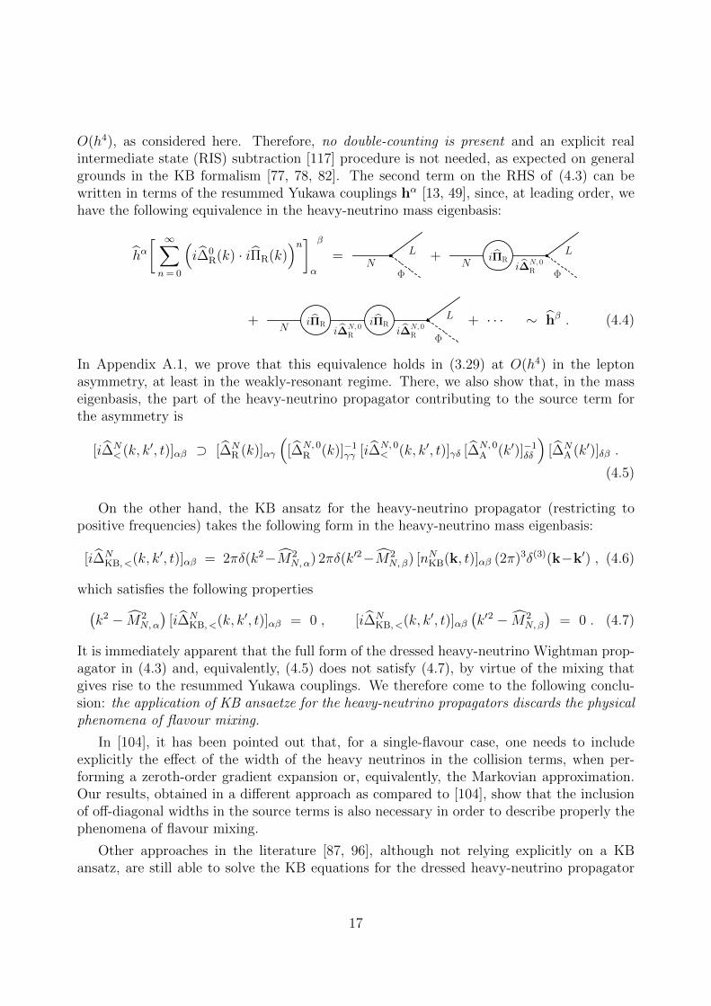
O(h4), as considered here. Therefore, no double-counting is present and an explicit realintermediate state (RIS) subtraction [117] procedure is not needed, as expected on generalgrounds in the KB formalism [77, 78, 82]. The second term on the RHS of (4.3) can bewritten in terms of the resummed Yukawa couplings hα [13, 49], since, at leading order, wehave the following equivalence in the heavy-neutrino mass eigenbasis:

hα[ ∞∑

n= 0

(i∆0

R(k) · iΠR(k))n] β

α

=N

L

Φ

+ LN i∆N, 0

R Φ

iΠR

+N

L

i∆N, 0R i∆N, 0

R Φ

iΠR iΠR + · · · ∼ hβ . (4.4)

In Appendix A.1, we prove that this equivalence holds in (3.29) at O(h4) in the leptonasymmetry, at least in the weakly-resonant regime. There, we also show that, in the masseigenbasis, the part of the heavy-neutrino propagator contributing to the source term forthe asymmetry is

[i∆N< (k, k′, t)]αβ ⊃ [∆N

R (k)]αγ

([∆N, 0

R (k)]−1γγ [i∆N, 0

< (k, k′, t)]γδ [∆N, 0A (k′)]−1

δδ

)[∆N

A (k′)]δβ .

(4.5)

On the other hand, the KB ansatz for the heavy-neutrino propagator (restricting topositive frequencies) takes the following form in the heavy-neutrino mass eigenbasis:

[i∆NKB, <(k, k′, t)]αβ = 2πδ(k2−M2

N,α) 2πδ(k′2−M2N, β) [nNKB(k, t)]αβ (2π)3δ(3)(k−k′) , (4.6)

which satisfies the following properties

(k2 − M2

N,α

)[i∆N

KB, <(k, k′, t)]αβ = 0 , [i∆NKB, <(k, k′, t)]αβ

(k′2 − M2

N, β

)= 0 . (4.7)

It is immediately apparent that the full form of the dressed heavy-neutrino Wightman prop-agator in (4.3) and, equivalently, (4.5) does not satisfy (4.7), by virtue of the mixing thatgives rise to the resummed Yukawa couplings. We therefore come to the following conclu-sion: the application of KB ansaetze for the heavy-neutrino propagators discards the physicalphenomena of flavour mixing.

In [104], it has been pointed out that, for a single-flavour case, one needs to includeexplicitly the effect of the width of the heavy neutrinos in the collision terms, when per-forming a zeroth-order gradient expansion or, equivalently, the Markovian approximation.Our results, obtained in a different approach as compared to [104], show that the inclusionof off-diagonal widths in the source terms is also necessary in order to describe properly thephenomena of flavour mixing.

Other approaches in the literature [87, 96], although not relying explicitly on a KBansatz, are still able to solve the KB equations for the dressed heavy-neutrino propagator

17

[i∆N< ]

βα

i∆Φ<

i∆L>

hα hβ ⊃ R A

[i∆N, 0< ] β

α

i∆Φ<

i∆L>

α β

'

[i∆N, 0< ] β

α

i∆Φ<

i∆L>

hα hβ

Figure 3: Diagrammatic representation of the source term for the charged-lepton asymmetryin terms of the resummed Yukawa couplings and the spectrally-free heavy-neutrino propaga-tor.

only up to an unknown function that parametrizes the external perturbation of the system.Both mixing and oscillations are in principle present in such double-time approaches. Itis however not clear whether our predictions are in quantitative agreement, since a directcomparison is made difficult by the simplified non-equilibrium setting in a non-expandingUniverse studied in [87, 96].

From (4.4), we see that the mixing effect due to the absorptive part of the heavy-neutrinoself-energy in the dressed propagator (4.3) can be factorized into the resummed Yukawacouplings. Moreover, we can replace the non-homogeneous free heavy-neutrino propagator∆N,0

< (k, k′, t) on the RHS of (4.3) with the homogeneous approximation given by (2.17).Thus, the contribution of the charged-lepton self-energy to the source term may be written interms of the spectrally-free heavy-neutrino propagator and the resummed Yukawa couplingshα as

dδnL

dt⊃ −

∫

k

θ(k0)[hβh

α(

[i∆N, 0< (k, t)] β

α Beq> (k)− [i∆N, 0

> (k, t)] βα Beq

< (k))− C.c.

], (4.8)

without having required a quasi-particle ansatz for the dressed heavy-neutrino propaga-tor. This procedure is illustrated diagrammatically in Figure 3 and proven explicitly inAppendix A.1.

Finally, assuming kinetic equilibrium7 and separating the CP -“even” and “-odd” partsof the heavy-neutrino number density nN and δnN , as described in [49], the equation forthe asymmetry becomes

dδnL

dt=

([nN ] β

α

nNeq

− δ βα

)[δγNLΦ]

α

β +[δnN ] β

α

2nNeq

[γNLΦ]α

β + W[δnL] , (4.9)

7 This is a valid assumption in the strong-washout regime of RL, since elastic scattering processes rapidlyequilibrate the momentum distributions for all the relevant particle species on time-scales much shorter thanthose of their statistical evolution.

18

where W[δnL] denotes the washout terms not studied explicitly here. The thermally-averaged rates are defined as

[γNLΦ] βα ≡

∫

NLΦ

(hαh

β + [hc]α[hc]β), (4.10a)

[δγNLΦ] βα ≡

∫

NLΦ

(hαh

β − [hc]α[hc]β), (4.10b)

where c ≡ CP indicates the generalized CP conjugate. Equation (4.9) describes the gen-eration of the asymmetry via both heavy-neutrino mixing (proportional to [δγNLΦ] β

α ) andoscillations (proportional to [δnN ] β

α ). In particular, the source terms agree with the onesgiven in [49], where both the phenomena are separately identified and taken into account inthe calculation of the final asymmetry.

5. Approximate Analytic Solution for the Lepton Asymmetry

In this section, we obtain an approximate analytic solution for the charged-lepton asym-metry in the strong-washout regime, using the KB rate equations derived in Section 3. Tothis end, we introduce the following notational conventions:

ηX ≡ nX

nγ, ηN ≡ ηN

ηNeq

− 1 , K ≡ Γ

ζ(3)HN

, (5.1)

where nγ = 2T 3ζ(3)/π2 is the photon number density (with ζ(3) ≈ 1.20206) and HN is theHubble constant in a Friedmann-Robertson-Walker Universe at temperature T = MN . Thethermal width Γ of the heavy neutrinos, obtained from Im ΠN

R = MNΓ, is related to the

decay rate by means of ΠN< (k0 > 0,k) ' 2i e−k0/T Im ΠN

R , which implies

ReγNLΦ =gN2

M3N K1(z) Γ

π2z, (5.2)

with z = MN/T and Kn(z) being the n-th order modified Bessel function of the second kind.We emphasize again that the off-diagonal elements of (5.2) induce flavour coherences in theheavy-neutrino sector via the second term on the RHS of (3.27a), giving rise to oscillationsby virtue of the flavour commutators in (3.27).

Taking into account the expansion of the Universe and using ηNeq ≈ gNz2K2(z)/4, (3.27a)

and (3.27b) can be combined into [49]

dηN

dz=

K1(z)

K2(z)

(1 + ηN − iz

[MN

ζ(3)HN

, ηN]− z

2

K, ηN

). (5.3)

In the strong-washout regime [K]αβ 1, the system evolves towards the attractor solutiongiven by

i

[MN

ζ(3)HN

, ηN]

+1

2

KN , ηN

' 12

z. (5.4)

19

The elements needed in what follows are found to be

[ηN ]αα =1

[K(0)]αα z

(MN, 1 −MN, 2)2 + (Γ(0)11 + Γ

(0)22 )2/4

(MN, 1 −MN, 2)2 +(Γ

(0)11 +Γ

(0)22 )2 Im[(h†h)12]2

4 (h†h)11(h†h)22

' 1

[K(0)]αα z, (5.5)

Im[ηN ]12 =ζ(3)HN

z

[Γ(0)]12

[Γ(0)]11[Γ(0)]22

(MN, 1 −MN, 2)(Γ(0)11 + Γ

(0)22 )/2

(MN, 1 −MN, 2)2 +(Γ

(0)11 +Γ

(0)22 )2 Im[(h†h)12]2

4 (h†h)11(h†h)22

, (5.6)

where Γ(0) is the thermal width matrix, appearing in (5.2), but with tree-level Yukawacouplings in γNLΦ. Taking into account the expansion of the Universe and neglecting 2 ↔ 2scatterings in the washout term, the rate equation for the lepton asymmetry (4.9) can bewritten as [49]

d[δηL]

dz= z3K1(z)

[− 1

3K δηL

+π2z

M3NK1(z)2ζ(3)HN

(Im[ηN ]12 Im[γNLΦ]12 + [ηN ]αβ [δγNLΦ]βα

)], (5.7)

where K = Tr K is an effective washout parameter. The attractor solution is found bysetting the RHS of (5.7) to zero. We also neglect the O(h6) off-diagonal entries in the lastterm, finally obtaining

δηL ' δηLmix + δηLosc , (5.8)

where the neglected terms in (5.8) are formally at O(h6) and higher. Here, the mixing andoscillation contributions are given explicitly by

δηLmix =gN2

3

2Kz

∑

α 6=β

Im(h†h)2

αβ

(h†h)11(h†h)22

(M2

N,α −M2N, β

)MN Γ

(0)ββ(

M2N,α −M2

N, β

)2+(MN Γ

(0)ββ

)2 , (5.9)

δηLosc =gN2

3

2Kz

Im(h†h)2

12

(h†h)11(h†h)22

(M2

N, 1 −M2N, 2

)MN

(Γ

(0)11 + Γ

(0)22

)(M2

N, 1 −M2N, 2

)2+ M2

N(Γ(0)11 + Γ

(0)22 )2 Im[(h†h)12]2

(h†h)11(h†h)22

.

(5.10)

These results, valid in the weakly-resonant strong-washout regime, exactly reproduce theones obtained in the semi-classical Boltzmann approach of [49] for the single lepton flavourcase studied here. At leading order, the contribution of mixing is governed by the diagonalentries of the CP -“even” number density nN , whereas that of oscillations is triggered by thepresence of off-diagonal CP -“odd” δnN . A detailed discussion of both flavour mixing andoscillations, in relation to the CP -violation properties of the Lagrangian of the system, isgiven in [49].

We note here that the oscillation term in (5.10) by itself agrees with the form for thetotal asymmetry given in the quantum Boltzmann approach of [97] and with earlier results

of [86, 87, 94, 95] in their validity limit Re[(h†h)212] (h†h)αα.8 Moreover, this oscillation

8 The limit Re[(h†h)212] (h†h)αα implies that Im[(h†h)12]2 ' (h†h)11(h†h)22 in the two-flavour case.

20

0.2 0.5 110

-8

10-7

10-6

z = mNT

∆Η

L

∆ΗL

∆Ηmix

L

∆Ηosc

L

Figure 4: The evolution of the total asymmetry (black continuous line), starting from theinitial conditions ηN = 2 ηNeq12 and δηL = 0. The red dotted line is the contribution offlavour mixing and the blue dashed line is that of oscillations. For illustrative purposes,the parameters are chosen as follows: mN = 1 TeV, (mN, 2 − mN, 1)/mN = 10−12, h1 =

0.5 × 10−6 (1 + 5 eiδ)mN and h2 = 0.5 i × 10−6 (1 − 5 eiδ)mN , with δ = 2 × 10−5. Forsimplicity, the effect of thermal masses and widths is neglected.

phenomenon does not involve any off-shell effects, since (5.10) can be obtained from anon-shell analysis with only tree-level Yukawa couplings (see [49]). However, unlike previoustreatments, we emphasize that the KB approach detailed in this paper captures the distinctphenomena of flavour mixing [11–16] in addition to oscillation phenomena. As shown nu-merically in [49], the contributions of these two distinct flavour effects, (5.9) and (5.10), arecomparable in the weakly-resonant regime. Hence, the total lepton asymmetry in (5.8) canbe enhanced by a factor of order two, compared to either (5.9) or (5.10) alone.

In order to illustrate the distinction between the two physical phenomena contributingto the generation of the asymmetry, we plot in Figure 4 the numerical solution of the rateequations (5.3) and (5.7), starting from the initial conditions ηN = 2 ηNeq12 and δηL = 0. Theblack continuous line denotes the solution of the full rate equations, the red dotted line givesthe contribution of mixing (obtained neglecting off-diagonal number densities) and the bluedashed line shows the contribution of oscillations (obtained replacing hα → hα). With thischoice of initial conditions, coherences between the two heavy-neutrino flavours are initiallyabsent. Thus, at early times, only flavour mixing contributes to the asymmetry. On theother hand, as discussed in detail in [49], in order to have a significant contribution fromoscillations, the off-diagonal entry nN12 needs first to be created by coherent decays and inverse

21

decays. Thus, as shown in Figure 4, this phenomenon becomes effective later than flavourmixing. At late times, both phenomena are present and give a similar contribution in theweakly-resonant strong-washout regime, providing an enhancement by a factor of order twowith respect to mixing or oscillations alone. The different time behaviour outlined above,in addition to their differing physical origins, confirms that mixing and oscillations are twodistinct physical phenomena and that both their contributions to the asymmetry need tobe taken into account. Finally, we point out that the oscillatory behaviour in Figure 4 doesnot result from non-Markovian memory effects as studied, for example, in [73, 74]. Instead,it is due to the oscillation of the heavy-neutrino coherences. The non-Markovian finite-timeeffects are safely neglected in the strong-washout regime of interest here.

Before concluding this section, we would like to stress here that the phenomenon ofcoherent heavy-neutrino oscillations, discussed above, is an O(h4) effect on the total leptonasymmetry [49] and so differs from the O(h6) mechanism proposed in [43]. The latter effectis relevant only at temperatures much higher than the sterile neutrino masses, such as inthe models studied in [32, 43–48, 88, 118], where the total lepton number is not violatedat leading order. On the other hand, the O(h4) effect identified here (and earlier in [49]) isenhanced in the same regime as the resonant ε-type CP violation effects, namely for z ≈ 1and ∆MN ∼ ΓNα , and its contribution to the final lepton asymmetry depends cruciallyon the flavour coherences in the heavy-neutrino sector (cf. (4.9); see [49] for a detaileddiscussion). In the current work, we have assumed that the momentum distribution inkinetic equilibrium is a flavour singlet. As discussed in [49], this approximation is valid inthe resonant regime, but not in the hierarchical one. A detailed study of this phenomenonin the hierarchical regime goes beyond the scope of this paper and will be given elsewhere.

6. Conclusions

We have presented a novel approach to the study of flavour effects in Resonant Lepto-genesis by embedding the fully flavour-covariant formalism developed in [49] into the per-turbative non-equilibrium thermal field theory formulated in [115]. In this formulation, onemay expand the Schwinger-Dyson series diagrammatically in a perturbative loopwise sense,without encountering pinch singularities. Moreover, one may define physically-meaningfulnumber densities at any order in perturbation theory, without necessitating the use of anyquasi-particle ansatz. The truncation of the resulting transport equations proceeds in atwo-fold manner: (i) spectrally, corresponding to the choice of observables being counted inthe quantum transport equation and (ii) statistically, by which the set of processes causingthe non-equilibrium evolution of the system are fixed.

Within this perturbative non-equilibrium field-theoretical framework, we have confirmedthe results previously obtained in [49] via a semi-classical formalism, reproducing themquantitatively at O(h4) in the weakly-resonant regime. The main physical result is that themixing of different heavy-neutrino flavours and the oscillations between them are two distinctphysical phenomena. The first is driven by the CP -“even” number density nN and the CP -“odd” rate [δγNLΦ] β

α , whereas the second is mediated by the CP -“odd” off-diagonal coherences

22

[δnN ]12. This is akin to the mixing and oscillation phenomena observed experimentally inK, D and B-meson systems. As identified in [49], both the phenomena contribute at O(h4)with comparable magnitude in the weakly-resonant regime. The strong-washout form of theasymmetry due to oscillations (5.10) is in agreement with the results obtained in other KBstudies [86, 87, 94, 97] and in the flavour-covariant semi-classical approach in [49].

However, as emphasized throughout this article, the KB approach presented here includesalso the effect of mixing, as given by (5.9). This contribution agrees with the one identified in[12], and re-obtained in [13, 49], once the thermal masses and widths are used in the formulaegiven there. The appearance of this additional O(h4) contribution, not present in previousKB studies, is due to the fact that we do not, as is typically the case, use a KB ansatz,or other equivalent approximations, for the dressed heavy-neutrino propagators. We haveshown that these approximations implicitly discard mixing effects. In the approach detailedhere, such approximations are not required, since we are able to express the source term forthe asymmetry in terms of the spectrally-free heavy-neutrino propagators, with the effect ofmixing being captured by the effective resummed Yukawa couplings [cf. (4.8)]. In Figure 4,we have shown explicitly that mixing and oscillations are two distinct physical phenomenathat contribute separately to the asymmetry, since their time behaviour, in addition to theirphysical origin, is different. With this approach to solving the quantum transport equations,we have justified, at leading order in the weakly-resonant regime, the semi-classical approachadopted in [49] of describing the effect of mixing by means of effective CP -violating Yukawacouplings [13]. Finally, we emphasise that mixing and oscillation contributions to the BAUare not exclusive to leptogenesis but generic phenomena applicable to baryogenesis modelsinvolving mixing of states. Therefore, both contributions should be included for precisequantitative predictions of the generated baryonic asymmetry in the Universe.

Acknowledgments

The authors would like to thank Bjorn Garbrecht for critical reading of the manuscript.D.T. would also like to thank Alexander Kartavtsev for discussions. The work of P.S.B.D.and A.P. is supported by the Lancaster-Manchester-Sheffield Consortium for FundamentalPhysics under STFC grant ST/J000418/1. The work of P.M. is supported by a UniversityFoundation Fellowship (TUFF) from the Technische Universitat Munchen and by the DFGcluster of excellence ‘Origin and Structure of the Universe’. This work was also supported inpart by the IPPP under STFC grant ST/G000905/1. The work of D.T. has been supportedby a fellowship of the EPS Faculty of the University of Manchester.

Appendix A. Resummed Thermal Propagators and Yukawa Couplings

In [49], it was shown that the time-translational invariance of flavour-covariant CTPpropagators is necessarily broken in the absence of thermodynamic equilibrium. In this sec-tion, working within the Markovian approximation detailed in Sections 3 and 4, we derive

23

the momentum-space representation of the resummed CTP propagator in the mass eigen-basis. Subsequently, in Appendix A.1, we use the form of these resummed propagators toobtain the resummed Yukawa couplings in the presence of thermal corrections. In so doing,we generalize the approach of [13]. Finally, in Appendix A.2, we reproduce the thermalRIS contribution used in the semi-classical approach of [49]. Throughout this appendix, wesuppress the superscript N on heavy-neutrino propagators and self-energies for notationalconvenience.

In coordinate space, the resummed heavy-neutrino CTP propagator takes the form

[i∆ab(x, y, tf ; ti)]βα ≡ 〈TC[Na

α(x)N b, β(y)]〉t , (A.1)

where TC denotes path ordering along the CTP contour (see Figure 1), a, b = 1, 2 arethe CTP indices (see [69–71]) and the heavy-neutrino field operators are understood in theHeisenberg picture. We note that (A.1) is not a picture-independent object, since it is notevaluated at equal times x0 = y0 = tf (see [115]). In what follows, we work in momentumspace, omitting all arguments for conciseness.

In the thermal mass eigenbasis (see Section 2), we may write the inverse resummed CTP

propagator ∆−1 in the following block decomposition:

∆−1 =

[D −D<

−D> D

](A.2)

where the set of submatrices D have elements given by (see e.g. [13])

Dαβ = (p2 − M2α) δαβ + iε(δαβ + 2nαβ) + [Πabs]αβ , (A.3a)

D≷, αβ = 2iε(θ(± p0)δαβ + nαβ

)+ [Π≷]αβ , (A.3b)

Dαβ = − (p2 − M2α) δαβ + iε(δαβ + 2nαβ) − [Π∗abs]αβ . (A.3c)

Here, Mα is the thermal mass, defined via (2.14), and [Πabs]αβ are the elements of the absorp-tive part of the Feynman self-energy. We omit the caret on D’s for notational convenience.The terms proportional to the prescription ε (cf. [115]) are, as we will see, necessary to obtainthe correct tree-level propagators and results consistent with the diagrammatic resummationin Section 4. We note that the matrix inversion of the inverse propagator does not yielda unique solution to the Klein-Gordon equation without correctly encoding the boundaryconditions of the Cauchy problem by virtue of these prescription-dependent terms.

The inverse CTP propagator (A.2) transforms as a rank-2 tensor of U(N ) under anarbitrary flavour rotation U, as follows:

[∆−1] lk = [U † ∆−1 U ] l

k (A.4)

where U ∈ U(N ) and can be written as a Kronecker product

U ≡ 12 ⊗ U , (A.5)

24

in which 12 is the 2×2 unit matrix. In addition, the CTP indices of ∆−1 in (A.4) are raisedand lowered by means of the SO(1, 1) CTP ‘metric’

g = gab ≡ diag(1,−1) , (A.6)

as follows:[∆−1]ab = [g ∆−1 g]ab , (A.7)

whereg ≡ g ⊗ 12 . (A.8)

Notice that the choice of block decomposition is not unique. We could alternatively havechosen to represent the inverse CTP propagator in the form

[∆−1]′ ≡[D11 D12

D21 D22

], (A.9)

where

Dαβ =

[Dαβ −D<,αβ

−D>,αβ Dαβ

]. (A.10)

In this case, the order of the Kronecker products in the 2N × 2N U(N ) and SO(1, 1)transformation matrices would be reversed, i.e.

U ≡ U ⊗ 12 , g ≡ 12 ⊗ g . (A.11)

Nevertheless, the two block decompositions (A.4) and (A.9) are related by means of a per-mutation transformation, i.e. [∆−1]′ = P∆−1P. For example, in the relevant case N = 2,the involutory permutation matrix P is given by

P =

1 0 0 00 0 1 00 1 0 00 0 0 1

. (A.12)

Therefore, both choices of block decomposition will yield equivalent results for the resummedCTP propagator, since these will be related by the same transformation, i.e. ∆′ = P∆P.

By virtue of the Banachiewicz inversion formula, the block decomposition of the re-summed CTP propagator is

∆ ≡ [∆]ab =

[ (∆−1/D

)−1 (∆−1/D<

)−1

(∆−1/D>

)−1 (∆−1/D

)−1

], (A.13)

where A/B denotes the Schur complement of A relative to B, i.e.

∆−1/D = D − D<D−1D> , ∆−1/D = D − D>D

−1D< , (A.14a)

∆−1/D> = D< − DD−1> D , ∆−1/D< = D> − DD−1

< D . (A.14b)

25

The resummed CTP propagator then takes the form

∆ =1

det ∆−1

[DDD DDD<

DDD> DDD

], (A.15)

where

DDD ≡ D adj(D − D<D

−1D>

), DDD ≡ D adj

(D − D>D

−1D<

), (A.16)

DDD> ≡ D> adj(D< − DD−1

> D), DDD< ≡ D< adj

(D> − DD−1

< D). (A.17)

Here, adj indicates the adjugate matrix and Roman (non-italicized) D’s denote the deter-minant of the corresponding matrix, e.g. for N = 2

D = detD = D11D22 − D12D21 . (A.18)

Using the relations for the retarded and advanced functions,

DR = D − D< = D> − D , (A.19a)

DA = D†R = D − D> = D< − D , (A.19b)

we may show that

DDD = − adj (DR)D adj (DA) , (A.20a)

DDD = − adj (DR)D adj (DA) , (A.20b)

DDD≷ = − adj (DR)D≷ adj (DA) . (A.20c)

The determinant of the inverse CTP propagator may be calculated using elementary rowtransformations and is given by

det ∆−1 = (−1)N DRDA = (−1)NDRD∗R = (−1)N |DR|2. (A.21)

Finally, putting everything back together, we find the following form for the resummedCTP propagators in the case of N flavours:

∆F = (−1)N−1∆RD∆A , (A.22a)

∆D = (−1)N−1∆RD∆A , (A.22b)

∆≷ = (−1)N−1∆RD≷∆A , (A.22c)

where

∆R = D−1R =

adjDR

DR

, ∆A = D−1A =

adjDA

DA

(A.23)

are the retarded and advanced propagators, respectively. We note that the expressions(A.22) are fully flavour-covariant and can be rotated to any basis. In addition, one mayverify that

∆R(A) = ∆F − ∆<(>) = ∆>(<) − ∆D , (A.24)

26

consistent with a single-flavour scenario.

In addition, we note that by virtue of the contributions from the ε-dependent termsin (A.3), the resummed propagators in (A.22) are consistent with those obtained by theiterative diagrammatic resummation in (4.3). For instance, consider the ε-dependent con-tribution to the Wightman propagators

i[∆≷]αβ ⊃ [∆R]αγ2ε(θ(±p0)δγδ + nγδ

)[∆A]δβ . (A.25)

This may be written as

i[∆≷]αβ ⊃ [∆R]αγ[∆0,−1R ]γσ[∆0

R]σσ2ε[θ(±p0)δσρ + nσρ][∆0A]ρρ[∆

0,−1A ]ρδ[∆A]δβ , (A.26)

where the central terms are given by

[∆0R]σσ2ε[θ(±p0)δσρ + nσρ][∆

0A]ρρ =

1

p2 − Mσ + iεp0

2ε[θ(±p0)δσρ + nσρ]1

p2 − Mρ − iεp0

.

(A.27)

In the homogeneous Markovian approximation, we replace Mσ ∼ Mρ ≈ M . Thus, using thelimit representation of the Dirac delta function

δ(x) = limε→0+

1

π

ε

x2 + ε2, (A.28)

we find

i[∆0≷]σρ = [∆0

R]σσ2ε[θ(±p0)δσρ + nσρ][∆0A]ρρ = 2πδ(p2 − M2)[θ(±p0)δσρ + nσρ] , (A.29)

which is precisely the propagator in (2.17). Hence, (A.26) yields the second line of (4.3).

Having observed that it is not appropriate to neglect the ε-dependent terms next to theself-energies in (A.3), it is pertinent to comment on the NWA of the resummed propagators.At first sight, it would appear that both lines of (4.3) give two identical contributionsin the NWA. However, we point out that ε and η ≡ ImΠR → 0 should be treated as twoindependent infinitesimals, since the latter is, strictly speaking, small but finite in the NWA.Thus, in this approximation, the first line of (4.3) is proportional to η, whereas the secondline to ε [see (A.29)]. Combining them, we obtain a term of the form

limε,η→0+

1

π

ε+ η

x2 + (ε+ η)2= δ(x) , (A.30)

which shows that we recover the expected result in the NWA.

In addition, it is illustrative to check that we recover the correct zero-temperature andsingle-flavour CTP limits. As an example, we consider the flavour-11 component of theresummed Feynman propagator. In the zero-temperature limit, we may restrict to positivefrequencies, setting ∆< = 0, such that ∆R → ∆F and ∆A → − ∆D. For N = 2, we thenfind

[∆F]11 =D22

D=[D11 − D12D

−122 D21

]−1

(A.31)

27

which, in the mass eigenbasis, gives

[∆F]11 =

[p2 − M2

1 + iε + Π11 −Π12Π21

p2 − M22 + iε + Π22

]−1

(A.32)

in agreement with well-known results (see e.g. [11]).

On the other hand, we may obtain the single flavour limit by setting the off-diagonalcomponents (D12, D21, ∆12, ∆21, etc.) to zero. In this case, we obtain the usual CTPresummed propagator

∆F = − D11

|DR, 11|2, (A.33)

which, after dropping the redundant flavour indices, takes the form

∆F =p2 − M2 − iIm Π(p)

(p2 − M2)2 + (Im Π(p))2, (A.34)

with M2 = m2−Re Π(p). Notice that we have safely dropped the ε-dependent terms, againin agreement with known results (see e.g. [115]).

Appendix A.1. Resummed Yukawa Couplings in Charged-Lepton Self-Energies

In this subsection, we show explicitly that, formally at O(h4) in the asymmetry, thecontribution of the charged-lepton self-energy to the source term can be written in terms ofthe resummed Yukawa couplings, as in (4.8) and illustrated in Figure 3.

From (4.9), we see that the quantity of interest is

T ≡ hα [∆<] βα hβ . (A.35)

The contribution to T of the second line of (4.3), which appears in the source term (4.9),will be denoted by Tsrc. Using (4.3) and noting that the summations there are equal to∆R(A) ·∆0,−1

R(A), Tsrc can be written as

Tsrc = hα [∆R] λα [∆0,−1

R ] γλ [∆0

<] δγ [∆0,−1

A ] µδ [∆A] βµ hβ

=∑

γ,δ

hα [∆R]αγ

([∆0,−1

R ]γγ [∆0<]γδ [∆0,−1

A ]δδ

)[∆A]δβ hβ

≡ hα [∆R]αγ Nγδ [∆A]δβ hβ . (A.36)

Let us introduce the notation

/α ≡

2 if α = 1

1 if α = 2. (A.37)

We treat the off-diagonal number densities [nN ]α/α as formally at O(h2), assuming that theyare generated dynamically from an incoherent initial condition (see [49]). Therefore, we have

Nαβ = (s−M2N,α) [∆0

<]αβ (s−M2N, β) = (s− sα) [∆0

<]αβ (s− s∗β) + O(h4) , (A.38)

28

where we have used Γα,/α[∆0<]α/α = O(h4), with Γα being the width of the heavy neutrinos.

Here, sα denotes the location of the two complex poles of the retarded propagator

sα = M2N,α − iMNΓα . (A.39)

Proceeding as in [13], the resonant terms in Tsrc can be expanded as

Tsrc '∑

α

hαZα

s− sα

(Gα −

DR12

DR/α/α

G/α

), (A.40)

withGα ≡ Nαδ [∆A]δβ hβ . (A.41)

In (A.40), we have included the wavefunction renormalization Zα ≡(

dds

[∆R(s)]−1αα

)−1, even

though this will be a higher-order effect in the analysis below.

For the case of two heavy neutrinos studied here, the resummed Yukawa couplings aregiven, in the mass eigenbasis, by

hα = hα − h/α i Im[ΠR]α/α

M2N,α −M2

N, /α + i Im[ΠR]/α/α, (A.42)

where the indices are not summed over. The CP conjugate couplings [hc]α are obtained byusing the complex-conjugate tree-level couplings in the RHS of (A.42). Equation (A.41)can, in turn, be expanded as

Gα '∑

β

(Nαβ +

DR12

DR, ∗/β/β

Nα/β)

Z∗βs− s∗β

hβ . (A.43)

Using (A.43) in (A.40), we find

Tsrc =∑

α,β

hαZα

s− sαNαβ

Z∗βs− s∗β

hβ (A.44)

+∑

α,β

DR12

DR, ∗/β/β

hαZα

s− sαNα/β

Z∗βs− s∗β

hβ −∑

α,β

DR12

DR/α/α

hαZα

s− sαN/αβ

Z∗βs− s∗β

hβ + O(h6) .

The contributions in the second line of (A.44) can be neglected. To show this, consider forexample the first summation: the only terms that can give contributions at O(h4) are theones with α = /β. Using (A.38), these become

DR12

DR, ∗/β/β

hα [∆0<]αα

s− sαs− s∗β

hβ + O(h6) =DR

12

DR, ∗/β/β

hα [∆0<]αα iMNΓα hβ

M2N,α −M2

N, β − iMNΓβ+ O(h6) = O(h6) ,

(A.45)having also used (2.17) and (A.39). Therefore, we obtain the final expression

Tsrc =∑

α,β

hα [∆0<] βα hβ + O(h6) , (A.46)

which is the form that we use in (4.8) and Figure 3.

29

Appendix A.2. RIS in Semiclassical Boltzmann Approaches

We now use the results obtained above to recover the thermal RIS contribution usedin [49], relevant to semi-classical approaches. Let us consider the pole expansion of theFeynman propagator, which may be written in the form

∆F =DDD

|DR|2. (A.47)

For the flavour-11 component, the pole expansion is

[∆F]11 =D11

|DR|2∣∣∣∣s≈s1

+D11

|DR|2∣∣∣∣s≈s∗1

+D11

|DR|2∣∣∣∣s≈s2

+D11

|DR|2∣∣∣∣s≈s∗2

+ · · · , (A.48)

where s(∗)1,2 are the complex roots of |DR|2 = 0. Noting that

detDDD = − det[adj(DR)D adj(DA)

]= − |DR|2(N−1)detD , (A.49)

it follows, in the vicinity of the poles, that

detDDD = D11D22 − D12D21 ≈ 0 . (A.50)

Hence, we may write

[∆F]11 =D11

|DR|2∣∣∣∣s≈s1

+D11

|DR|2∣∣∣∣s≈s∗1

+D12

D22

D22

|DR|2D21

D22

∣∣∣∣s≈s2

+D12

D22

D22

|DR|2D21

D22

∣∣∣∣s≈s∗2

+ · · · , (A.51)

or, equivalently,

[∆F]11 =ZR, 1

s− s1

+ZA, 1

s− s∗1+

D12

D22

ZR, 2

s− s2

D21

D22

+D12

D22

ZA, 2

s− s∗2D21

D22

+ · · · , (A.52)

where we have introduced

ZR(A), α ≡ [ZR(A)(√s)]α =

(DA(R)(

√s)

2√s

d

d√s

[∆−1F (√s)]αα

DA(R)(√s)

)−1

. (A.53)

The pole expansion (A.52) differs from that in [13] by the presence of the complex-conjugatepoles. Proceeding similarly, we find

[∆F]22 =ZR, 2

s− s2

+ZA, 2

s− s∗2+

D21

D11

ZR, 1

s− s1

D12

D11

+D21

D11

ZA, 1

s− s∗1D12

D11

+ · · · , (A.54)

[∆F]12 =ZR, 1

s− s1

D12

D11

+ZA, 1

s− s∗1D12

D11

+D12

D22

ZR, 2

s− s2

+D12

D22

ZA, 2

s− s∗2+ · · · , (A.55)

[∆F]21 =ZR, 2

s− s2

D21

D22

+ZA, 2

s− s∗2D21

D22

+D21

D11

ZR, 1

s− s1

+D21

D11

ZA, 1

s− s∗1+ · · · . (A.56)

30

Finally, the amplitude pertinent to the derivation of the resummed Yukawa couplings insemi-classical approaches is the s-channel exchange [13] 9

Ts = ΓA1 [∆F ]11 ΓB1 + ΓA1 [∆F ]12 Γ

B2 + ΓA2 [∆F ]21 Γ

B1 + ΓA2 [∆F ]22 Γ

B2 . (A.57)

Using the results above, the resonant contribution takes the form

Ts = |V A1 |2[ |ZR, 1|2 + |ZA, 1|2

|s− s1|2+

ZR, 1Z∗A, 1

(s− s1)2+

Z∗R, 1ZA, 1

(s− s∗1)2

]|V B1 |2 + (1↔ 2) , (A.58)

where

VA(B)

1 = ΓA(B)1 +

D12

D11

ΓA(B)2 , V

A(B)2 = Γ

A(B)2 +

D21

D22

ΓA(B)1 . (A.59)

In the pole-dominance region, we find

|Ts,RIS|2 = |V A1 |2|V B1 |2π

m1ΓR, 1

|ZR, 1 − ZA, 1|2δ+(s− M21 ) + (1↔ 2) , (A.60)

where M21 = Re s1 = Re ΠR, 11 and M1ΓR, 1 = Im s1 = Im ΠR, 11 are the thermal masses

and widths, calculated from the dispersive and absorptive parts of the retarded self-energies,respectively. In addition, δ+(s − M2

1 ) = θ(√s)δ(s − M2

1 ). Notice that (A.60) is obtainedfrom the results of [13] by replacing |Zα|2 with |ZR, α − ZA, α|2 and the masses, widths andvertices by their thermal counterparts, calculated using the retarded self-energy.

Finally, we now show that, in the equilibrium limit, we recover the thermal RIS contri-bution found in [49]. Ignoring higher order mixing terms, we have

[∆F]11 ≈s− M2

1 + iMΓF,1(s− s1)(s− s∗1)

=s− M2

1 + i(1 + 2n(√s))MΓ1

(s− s1)(s− s∗1), (A.61)

using the fluctuation-dissipation theorem to relate the time-ordered and retarded widthsΓF, 1 and Γ1. Partial fractioning the resonant part, we obtain

[∆F]11 =iMΓ1

s1 − s∗1(1 + 2n(

√s))

[1

s− s1

− 1

s− s∗1

]. (A.62)

Since s1 − s∗1 = 2iMΓ1, we see the importance of keeping track of the structure of thenumerator and find

[∆F]11 =1

2(1 + 2n(

√s))

[1

s− s1

− 1

s− s∗1

]. (A.63)

9 Here, we have used A and B to label the vertices to avoid confusion with the A that denotes advancedfunctions.

31

In this case, the residues of the poles are

ZR, 1 =1

2(1 + 2n(

√s)) , ZA, 1 = − 1

2(1 + 2n(

√s)) . (A.64)

Hence, the RIS contribution takes the form

|Ts,RIS|2 = |V A1 |2|V B1 |2π

MΓ1

(1 + 2n(√s))2δ+(s− M2

1 ) + (1↔ 2) + · · · , (A.65)

which, to leading order in the statistical factors, contains the thermal RIS contributionidentified in [49]. As noted in Section 3, such thermal RIS contributions are not double-counted in the KB approach discussed in this article, but must be subtracted in semi-classicalBoltzmann approaches, such as [49]. Notice finally that, when the thermal contributions areneglected, (A.65) agrees with the results in [13].

References

[1] M. Fukugita and T. Yanagida, Phys. Lett. B 174 (1986) 45.[2] P. Minkowski, Phys. Lett. B 67, 421 (1977).[3] R. N. Mohapatra and G. Senjanovic, Phys. Rev. Lett. 44, 912 (1980).[4] M. Gell-Mann, P. Ramond and R. Slansky, Conf. Proc. C 790927, 315 (1979) [arXiv:1306.4669 [hep-

th]].[5] T. Yanagida, in Proceedings of the Workshop on Unified Theories and Baryon Number in the Universe,

eds. A. Sawada and A. Sugamoto, KEK, Tsukuba (1979).[6] J. Schechter and J. W. F. Valle, Phys. Rev. D 22, 2227 (1980).[7] K. A. Olive et al. (Particle Data Group), Chin. Phys. C 38, 090001 (2014) [http://pdg.lbl.gov/].[8] V. A. Kuzmin, V. A. Rubakov and M. E. Shaposhnikov, Phys. Lett. B 155 (1985) 36.[9] A. D. Sakharov, JETP Lett. 5 (1967) 24.

[10] S. Blanchet and P. Di Bari, New J. Phys. 14, 125012 (2012) [arXiv:1211.0512 [hep-ph]].[11] A. Pilaftsis, Nucl. Phys. B 504, 61 (1997) [hep-ph/9702393].[12] A. Pilaftsis, Phys. Rev. D 56, 5431 (1997) [hep-ph/9707235].[13] A. Pilaftsis and T. E. J. Underwood, Nucl. Phys. B 692, 303 (2004) [hep-ph/0309342].[14] M. Flanz, E. A. Paschos and U. Sarkar, Phys. Lett. B 345, 248 (1995) [Erratum-ibid. B 382, 447

(1996)] [hep-ph/9411366].[15] L. Covi, E. Roulet and F. Vissani, Phys. Lett. B 384, 169 (1996) [hep-ph/9605319].[16] W. Buchmuller and M. Plumacher, Phys. Lett. B 431, 354 (1998) [hep-ph/9710460].[17] A. Pilaftsis and T. E. J. Underwood, Phys. Rev. D 72, 113001 (2005) [hep-ph/0506107].[18] A. Pilaftsis, Phys. Rev. Lett. 95, 081602 (2005) [hep-ph/0408103].[19] F. F. Deppisch and A. Pilaftsis, Phys. Rev. D 83, 076007 (2011) [arXiv:1012.1834 [hep-ph]].[20] A. Datta, M. Guchait and A. Pilaftsis, Phys. Rev. D 50, 3195 (1994) [hep-ph/9311257].[21] T. Han and B. Zhang, Phys. Rev. Lett. 97, 171804 (2006) [hep-ph/0604064].[22] S. Bray, J. S. Lee and A. Pilaftsis, Nucl. Phys. B 786, 95 (2007) [hep-ph/0702294 [HEP-PH]].[23] A. Atre, T. Han, S. Pascoli and B. Zhang, JHEP 0905, 030 (2009) [arXiv:0901.3589 [hep-ph]].[24] P. S. B. Dev, A. Pilaftsis and U. K. Yang, Phys. Rev. Lett. 112, 081801 (2014) [arXiv:1308.2209

[hep-ph]].[25] G. Bambhaniya, S. Goswami, S. Khan, P. Konar and T. Mondal, arXiv:1410.5687 [hep-ph].[26] A. Ilakovac and A. Pilaftsis, Nucl. Phys. B 437, 491 (1995) [hep-ph/9403398].[27] R. Alonso, M. Dhen, M. B. Gavela and T. Hambye, JHEP 1301, 118 (2013) [arXiv:1209.2679 [hep-ph]].[28] A. Pilaftsis, Int. J. Mod. Phys. A 14, 1811 (1999) [hep-ph/9812256].

32

[29] T. Endoh, T. Morozumi and Z. -h. Xiong, Prog. Theor. Phys. 111, 123 (2004) [hep-ph/0308276].[30] O. Vives, Phys. Rev. D 73, 073006 (2006) [hep-ph/0512160].[31] S. Blanchet, P. Di Bari, D. A. Jones and L. Marzola, JCAP 1301, 041 (2013) [arXiv:1112.4528 [hep-

ph]].[32] T. Asaka and M. Shaposhnikov, Phys. Lett. B 620, 17 (2005) [hep-ph/0505013].[33] J. R. Ellis, M. Raidal and T. Yanagida, Phys. Lett. B 546 (2002) 228 [hep-ph/0206300].[34] R. Barbieri, P. Creminelli, A. Strumia and N. Tetradis, Nucl. Phys. B 575, 61 (2000) [hep-ph/9911315].[35] A. Abada, S. Davidson, F. -X. Josse-Michaux, M. Losada and A. Riotto, JCAP 0604, 004 (2006)

[hep-ph/0601083].[36] E. Nardi, Y. Nir, E. Roulet and J. Racker, JHEP 0601, 164 (2006) [hep-ph/0601084].[37] A. Abada, S. Davidson, A. Ibarra, F. -X. Josse-Michaux, M. Losada and A. Riotto, JHEP 0609, 010

(2006) [hep-ph/0605281].[38] S. Blanchet and P. Di Bari, JCAP 0703, 018 (2007) [hep-ph/0607330].[39] S. Pascoli, S. T. Petcov and A. Riotto, Nucl. Phys. B 774, 1 (2007) [hep-ph/0611338].[40] G. C. Branco, A. J. Buras, S. Jager, S. Uhlig and A. Weiler, JHEP 0709, 004 (2007) [hep-ph/0609067].[41] A. De Simone and A. Riotto, JCAP 0702, 005 (2007) [hep-ph/0611357].[42] G. Sigl and G. Raffelt, Nucl. Phys. B 406, 423 (1993).[43] E. K. Akhmedov, V. A. Rubakov and A. Y. Smirnov, Phys. Rev. Lett. 81, 1359 (1998) [hep-

ph/9803255].[44] M. Shaposhnikov, JHEP 0808, 008 (2008) [arXiv:0804.4542 [hep-ph]].[45] J. S. Gagnon and M. Shaposhnikov, Phys. Rev. D 83, 065021 (2011) [arXiv:1012.1126 [hep-ph]].[46] T. Asaka, S. Eijima and H. Ishida, JCAP 1202, 021 (2012) [arXiv:1112.5565 [hep-ph]].[47] L. Canetti, M. Drewes, T. Frossard and M. Shaposhnikov, Phys. Rev. D 87, 093006 (2013)

[arXiv:1208.4607 [hep-ph]].[48] B. Shuve and I. Yavin, Phys. Rev. D 89, 075014 (2014) [arXiv:1401.2459 [hep-ph]].[49] P. S. B. Dev, P. Millington, A. Pilaftsis and D. Teresi, Nucl. Phys. B 886, 569 (2014) [arXiv: 1404.1003

[hep-ph]].[50] P. S. B. Dev, P. Millington, A. Pilaftsis and D. Teresi, arXiv:1409.8263 [hep-ph].[51] A. Pais and O. Piccioni, Phys. Rev. 100 (1955) 1487.[52] P. K. Kabir, The CP puzzle: strange decays of the neutral kaon, Academic Press (1968).[53] D. Boyanovsky and C. M. Ho, Phys. Rev. D 75 (2007) 085004 [hep-ph/0610036].[54] D. Boyanovsky and L. Lello, New J. Phys. 16 (2014) 063050 [arXiv:1403.6366 [hep-ph]].[55] D. Boyanovsky, Nucl. Phys. B 888, 248 (2014) [arXiv:1406.5739 [hep-ph]].[56] D. Boyanovsky, arXiv:1409.4265 [hep-ph].[57] T. Prokopec, M. G. Schmidt and S. Weinstock, Annals Phys. 314 (2004) 208 [hep-ph/0312110].[58] T. Prokopec, M. G. Schmidt and S. Weinstock, Annals Phys. 314 (2004) 267 [hep-ph/0406140].[59] G. Baym and L. P. Kadanoff, Phys. Rev. 124 (1961) 287.[60] L. Kadanoff and G. Baym, Quantum Statistical Mechanics, Benjamin, New York (1962).[61] J. P. Blaizot and E. Iancu, Phys. Rept. 359 (2002) 355 [hep-ph/0101103].[62] J. Berges, AIP Conf. Proc. 739 (2005) 3 [hep-ph/0409233].[63] J. M. Cornwall, R. Jackiw and E. Tomboulis, Phys. Rev. D 10, 2428 (1974).[64] G. Amelino-Camelia and S. Y. Pi, Phys. Rev. D 47, 2356 (1993) [hep-ph/9211211].[65] J. Berges, S. Borsanyi, U. Reinosa and J. Serreau, Annals Phys. 320, 344 (2005) [hep-ph/0503240].[66] A. Pilaftsis and D. Teresi, Nucl. Phys. B 874 (2013) 2, 594 [arXiv:1305.3221 [hep-ph]].[67] J. S. Schwinger, J. Math. Phys. 2, 407 (1961).[68] L. V. Keldysh, Zh. Eksp. Teor. Fiz. 47, 1515 (1964) [Sov. Phys. JETP 20, 1018 (1965)].[69] R. D. Jordan, Phys. Rev. D 33 (1986) 444.[70] E. Calzetta and B. L. Hu, Phys. Rev. D 35, 495 (1987).[71] E. Calzetta and B. L. Hu, Phys. Rev. D 37, 2878 (1988).[72] W. Buchmuller and S. Fredenhagen, Phys. Lett. B 483, 217 (2000) [hep-ph/0004145].[73] A. De Simone and A. Riotto, JCAP 0708, 002 (2007) [hep-ph/0703175].

33

[74] A. De Simone and A. Riotto, JCAP 0708, 013 (2007) [arXiv:0705.2183 [hep-ph]].[75] V. Cirigliano, A. De Simone, G. Isidori, I. Masina and A. Riotto, JCAP 0801, 004 (2008)

[arXiv:0711.0778 [hep-ph]].[76] A. Anisimov, W. Buchmuller, M. Drewes and S. Mendizabal, Annals Phys. 324, 1234 (2009)

[arXiv:0812.1934 [hep-th]].[77] M. Garny, A. Hohenegger, A. Kartavtsev and M. Lindner, Phys. Rev. D 80 (2009) 125027

[arXiv:0909.1559 [hep-ph]].[78] M. Garny, A. Hohenegger, A. Kartavtsev and M. Lindner, Phys. Rev. D 81, 085027 (2010)

[arXiv:0911.4122 [hep-ph]].[79] V. Cirigliano, C. Lee, M. J. Ramsey-Musolf and S. Tulin, Phys. Rev. D 81, 103503 (2010)

[arXiv:0912.3523 [hep-ph]].[80] A. Anisimov, W. Buchmuller, M. Drewes and S. Mendizabal, Phys. Rev. Lett. 104, 121102 (2010)

[arXiv:1001.3856 [hep-ph]].[81] M. Garny, A. Hohenegger and A. Kartavtsev, Phys. Rev. D 81 (2010) 085028 [arXiv:1002.0331 [hep-

ph]].[82] M. Beneke, B. Garbrecht, M. Herranen and P. Schwaller, Nucl. Phys. B 838, 1 (2010) [arXiv:1002.1326

[hep-ph]].[83] M. Beneke, B. Garbrecht, C. Fidler, M. Herranen and P. Schwaller, Nucl. Phys. B 843, 177 (2011)

[arXiv:1007.4783 [hep-ph]].[84] B. Garbrecht, Nucl. Phys. B 847, 350 (2011) [arXiv:1011.3122 [hep-ph]].[85] A. Anisimov, W. Buchmuller, M. Drewes and S. Mendizabal, Annals Phys. 326, 1998 (2011) [Erratum-

ibid. 338, 376 (2011)] [arXiv:1012.5821 [hep-ph]].[86] B. Garbrecht and M. Herranen, Nucl. Phys. B 861, 17 (2012) [arXiv:1112.5954 [hep-ph]].[87] M. Garny, A. Kartavtsev and A. Hohenegger, Annals Phys. 328, 26 (2013) [arXiv:1112.6428 [hep-ph]].[88] M. Drewes and B. Garbrecht, JHEP 1303 (2013) 096 [arXiv:1206.5537 [hep-ph]].[89] B. Garbrecht, Nucl. Phys. B 868 (2013) 557 [arXiv:1210.0553 [hep-ph]].[90] T. Frossard, M. Garny, A. Hohenegger, A. Kartavtsev and D. Mitrouskas, Phys. Rev. D 87, 085009

(2013) [arXiv:1211.2140 [hep-ph]].[91] M. Drewes, Int. J. Mod. Phys. E 22 (2013) 1330019 [arXiv:1303.6912 [hep-ph]].[92] B. Garbrecht and M. J. Ramsey-Musolf, Nucl. Phys. B 882 (2014) 145 [arXiv:1307.0524 [hep-ph]].[93] A. Hohenegger and A. Kartavtsev, arXiv:1309.1385 [hep-ph].[94] S. Iso, K. Shimada and M. Yamanaka, arXiv:1312.7680 [hep-ph].[95] S. Iso and K. Shimada, JHEP 1408, 043 (2014) [arXiv:1404.4816 [hep-ph]].[96] A. Hohenegger and A. Kartavtsev, JHEP 1407 (2014) 130 [arXiv:1404.5309 [hep-ph]].[97] B. Garbrecht, F. Gautier and J. Klaric, JCAP 1409 (2014) 09, 033 [arXiv:1406.4190 [hep-ph]].[98] H. A. Weldon, Phys. Rev. D 45 (1992) 352.[99] T. Altherr and D. Seibert, Phys. Lett. B 333 (1994) 149 [hep-ph/9405396].

[100] T. Altherr, Phys. Lett. B 341 (1995) 325 [hep-ph/9407249].[101] P. F. Bedaque, Phys. Lett. B 344 (1995) 23 [hep-ph/9410415].[102] I. Dadıc, Phys. Rev. D 59 (1999) 125012 [hep-ph/9801399].[103] C. Greiner and S. Leupold, Eur. Phys. J. C 8 (1999) 517 [hep-ph/9804239].[104] B. Garbrecht and M. Garny, Annals Phys. 327 (2012) 914 [arXiv:1108.3688 [hep-ph]].[105] J. Winter, Phys. Rev. D 32 (1985) 1871.[106] J. Berges and S. Borsanyi, Phys. Rev. D 74 (2006) 045022 [hep-ph/0512155].[107] B. Garbrecht and T. Konstandin, Phys. Rev. D 79 (2009) 085003 [arXiv:0810.4016 [hep-ph]].[108] M. Garny, A. Hohenegger and A. Kartavtsev, arXiv:1005.5385 [hep-ph].[109] A. Vlasenko, G. M. Fuller and V. Cirigliano, Phys. Rev. D 89 (2014) 105004 [arXiv:1309.2628 [hep-

ph]].[110] P. Lipavsky, V. Spicka and B. Velicky, Phys. Rev. B 34 (1986) 6933.[111] T. Bornath, D. Kremp, W. D. Kraeft and M. Schlanges, Phys. Rev. E 54 (1996) 3274.[112] M. Herranen, K. Kainulainen and P. M. Rahkila, JHEP 1012 (2010) 072 [arXiv:1006.1929 [hep-ph]].

34

[113] M. Herranen, K. Kainulainen and P. M. Rahkila, JHEP 1202 (2012) 080 [arXiv:1108.2371 [hep-ph]].[114] C. Fidler, M. Herranen, K. Kainulainen and P. M. Rahkila, JHEP 1202 (2012) 065 [arXiv:1108.2309

[hep-ph]].[115] P. Millington and A. Pilaftsis, Phys. Rev. D 88 (2013) 8, 085009 [arXiv:1211.3152 [hep-ph]].[116] P. Millington and A. Pilaftsis, Phys. Lett. B 724 (2013) 56 [arXiv:1304.7249 [hep-ph]].[117] E. W. Kolb and S. Wolfram, Nucl. Phys. B 172, 224 (1980) [Erratum-ibid. B 195, 542 (1982)].[118] L. Canetti, M. Drewes and B. Garbrecht, arXiv:1404.7114 [hep-ph].

35