sDTW: Computing DTW Distances using Locally Relevant Constraints

based on Salient Feature Alignments

K. Selçuk Candan, Maria Luisa SapinoXiaolan Wang, Rosaria Rossini

This work is supported by the NSF Grant 1043583 MiNC: NSDL Middleware for Network- and Context- aware Recommendations.

2

Dynamic Time Warping

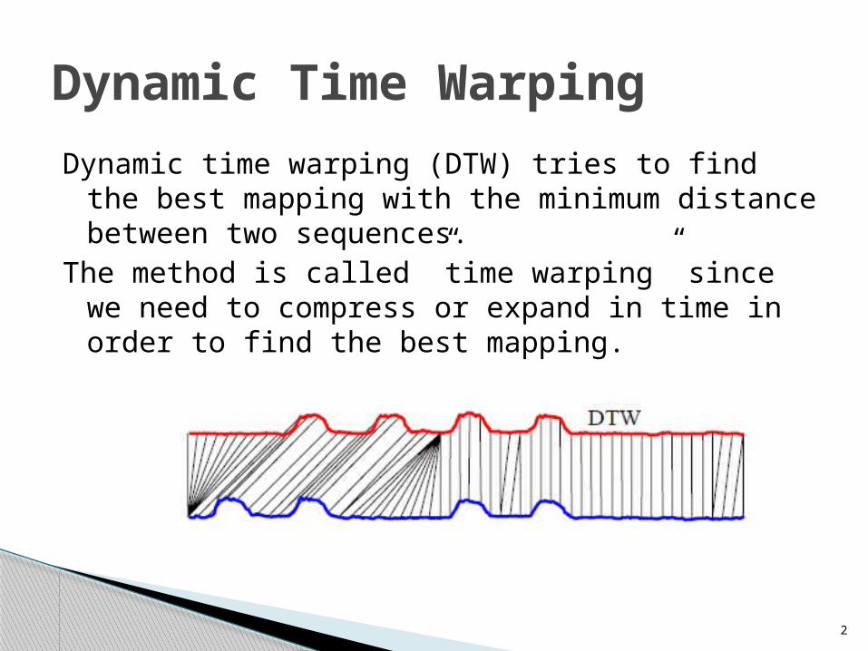
Dynamic time warping (DTW) tries to find the best mapping with the minimum distance between two sequences.

The method is called ”time warping” since we need to compress or expand in time in order to find the best mapping.

3

DTW Grid and Warp PathGiven two time series, X and Y, of length N and M,alternative warping strategies can be compactly representedas an NxM grid.

A warp path between X and Y then can be visualized as apath from the lower-left corner of the NxM grid to its

upper-right corner.

4

Reducing the cost of DTW

The major cost of the DTW algorithm is filling the NxM grid. To reduce cost, Sakoe and Chiba band constraints and Itakura Parallelogram define a narrow band around the diagonal from which the warp paths can pass.

5

sDTW Idea

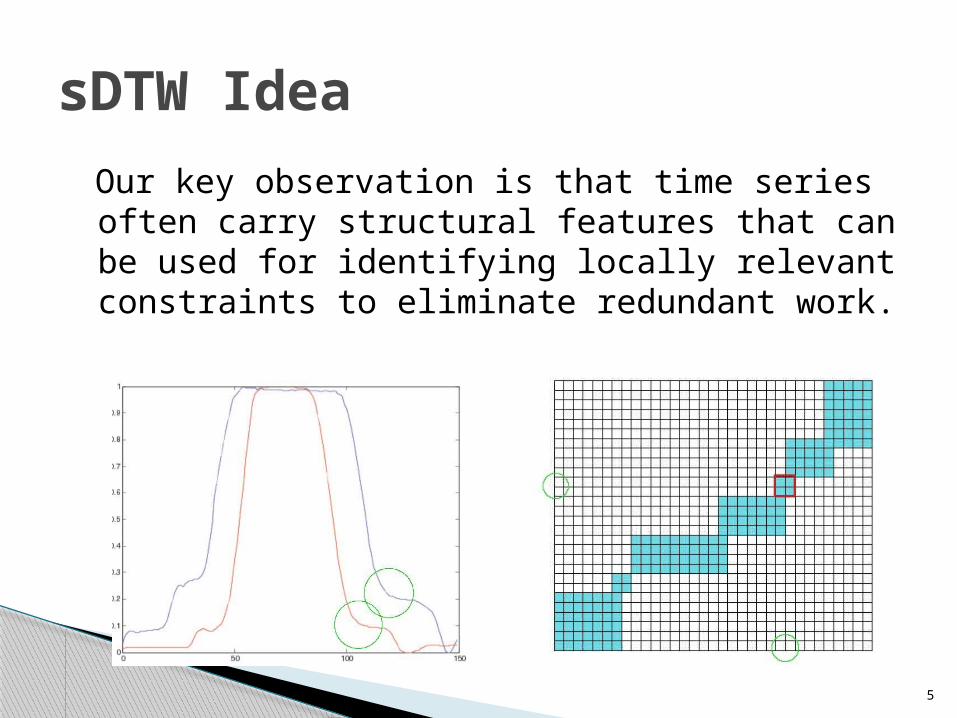
Our key observation is that time series often carry structural features that can be used

for identifying locally relevant constraints to eliminate redundant work.

6

Proposed Adaptive

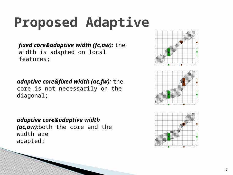
adaptive core&fixed width (ac,fw): thecore is not necessarily on the diagonal;

adaptive core&adaptive width(ac,aw):both the core and the width areadapted;

fixed core&adaptive width (fc,aw): thewidth is adapted on local features;

7

sDTW Process

1. Search for salient features on the input time series.

2. Find salient alignments of a given pair of time series by matching the descriptors of the salient features.

3. Use these salient alignments to compute locally relevant constraints to prune the warp path search.

sDTW leverages salient alignment evidences to improve the effectiveness of the pruning

constraints.

8

First Question

To search for robust local features, we adapt the scale-invariant feature transform (SIFT).

How can we locate robust local features of time series?

9

The scale-invariant feature transform (SIFT)4 is a computer vision algorithm used to detect and describe local features in 2D images.

The algorithm identifies salient point of a given image (and their descriptors) that are invariant to:

Image scaling; Translation; Rotation; Different illuminations and noise.

Scale-Invariant Feature Transform

We adapted the 2D SIFT algorithm in a way that captures characteristics of 1D time series.

10

The salient feature extraction algorithm relies on a three step process to identify such salient features and their robust local feature descriptors in time series:

Scale-space extrema detection; Feature descriptor creation. Feature filtering and localization

Each step is designed to capture characteristics of time series.

1D Scale-Invariant Feature Transform Steps

11

Salient Temporal Features

12

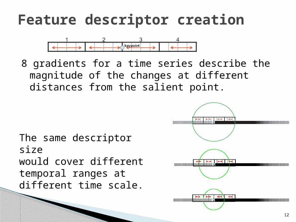
8 gradients for a time series describe the magnitude of the changes at different distances from the salient point.

Feature descriptor creation

The same descriptor sizewould cover different temporal ranges at different time scale.

13

I. the distance between the feature descriptors of each pair of salient features using Euclidean Distance;

II. the size of scopes between the features of the matching pairs.

2nd Step: Features Matching & Inconsistency Pruning

The Feature Matching Step is performed by compare:

A good match has less distance descriptors and similar size-scopes between two features.

14

Alignment feature pairs with large temporal length and close to each other in time;

Similarity pairs of features that have both similar descriptors and similar average amplitudes;

Combined score both allignment and similarity.

Inconsistency PruningFor each pair of matching features we look on:

15

Given two time series, consider the scopeboundaries of the pairs of matching salient features

in descending order of their μcomb scores and prunethose that imply inconsistent ordering of start and

end points.

Inconsistency Pruning

16

Inconsistency PruningPairs of matching salient points (pre-inconsistency removal)

Pairs of matches remaining after inconsistency pruning.

Scope boundariesof the matching salient features after inconsistency elimination

17

Locally Relevant DTW Constraints: WIDTH.

3trd Step of sDTW Process

A sets of matching consistent of salient

features after the inconsistent pruning.

Thus, our intuition is that each corresponding interval pair in the two time series corresponds to similar regions and thus must have similar characteristics.

18

Adaptive width constraints use the widths of the resulting intervals to choose a different

locally relevant width for eachpoint (details in the paper).

Adaptive Width Constrains

19

Locally Relevant DTW Constraints: CORE.

3trd Step of sDTW Process

Sample point alignmentswithin interval E.

We can use the starting and ending points of the corresponding intervals in the two time series to associate to each point in one series a candidate point in the other time series.

20

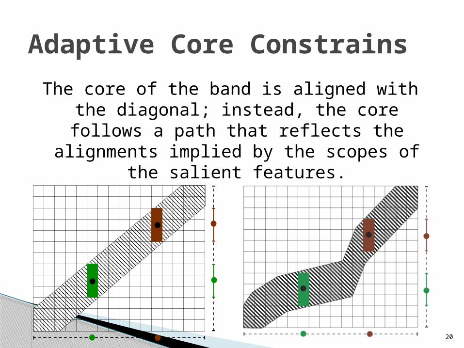
The core of the band is aligned with the diagonal; instead, the core follows a path

that reflects the alignments implied by the scopes of the salient features.

Adaptive Core Constrains

21

Adaptive Width Contraints can easely be combined with Adaptive Core Constraints.

Adaptive Core & Adaptive Width

22

For estimate the efficiency and effectiveness of sDTW, it is tested on the time series data sets:

Evaluation Criteria

Data Set Length # of Series

# of Classes

Gun 150 50 2

Trace 275 100 4

50Words 270 450 50

23

Intel Core 2 Quad CPU 3GHz machine, 8Gb RAM Ubuntu 9.10(64bit) Matlab 7.8.0

For the baseline fc&fw schemes we used the DTW code of Sakoe-Chiba.

Experiment Set Up

24

In order to assess the effectiveness of various DTW algorithms, we use the following measures:

Evaluation Criteria

Retrieval Accuracy

Distance accuracy

Classification accuracy

25

The overhead of the matching step for the adaptivealgorithms is negligible.

Execution Time Analysis

26

fixed core&fixed width (fc,fw) ⇒ the larger is the value of w, the more accurate the results are;

adaptive core&fixed width (ac,fw) ⇒ has significant gains in accuracy is obtained when the core is adapted;

adaptive core&adaptive width (ac,aw) ⇒ the accuracy is further boosted when both the width and the core are adapted.

Top-k Retrieval Accuracy

27

The figure re-confirms the results by focusing

on the classification accuracy.

Similarly to the top-k

retrieval and DTW distance accuracy

results, adaptive core, and adaptive width algorithmsimprove the classification

accuracy.

Classification Accuracy

28

The figure confirms the results by focusing on the errors inthe DTW estimates provided by the various algorithms forthe data set.

Distance Accuracy

29

We recognize that the time series that are being compared often carry structural evidences that

can help identify locally relevant constraints that can prune unnecessary work during dynamic time

warp (DTW) distance computation.

Experiment results have shown that the proposedlocally-relevant constraints based on salient

features help improve accuracy in DTW distance estimations.

Conclusions

We have proposed three different constraint types based on different assumptions on the

structural variations in the data set.

30

Thank you.