HAL Id: hal-01406473https://hal.archives-ouvertes.fr/hal-01406473v2

Submitted on 21 Aug 2017

HAL is a multi-disciplinary open accessarchive for the deposit and dissemination of sci-entific research documents, whether they are pub-lished or not. The documents may come fromteaching and research institutions in France orabroad, or from public or private research centers.

L’archive ouverte pluridisciplinaire HAL, estdestinée au dépôt et à la diffusion de documentsscientifiques de niveau recherche, publiés ou non,émanant des établissements d’enseignement et derecherche français ou étrangers, des laboratoirespublics ou privés.

Distributed under a Creative Commons Attribution - NonCommercial - NoDerivatives| 4.0International License

K Nearest Neighbour Joins for Big Data on MapReduce:A Theoretical and Experimental Analysis

Ge Song, Justine Rochas, Lea Beze, Fabrice Huet, Frederic Magoules

To cite this version:Ge Song, Justine Rochas, Lea Beze, Fabrice Huet, Frederic Magoules. K Nearest Neighbour Joins forBig Data on MapReduce: A Theoretical and Experimental Analysis. IEEE Transactions on Knowledgeand Data Engineering, Institute of Electrical and Electronics Engineers, 2016, 28 (9), pp.2376-2392.�10.1109/TKDE.2016.2562627�. �hal-01406473v2�

1

K Nearest Neighbour Joins for Big Data onMapReduce: a Theoretical and Experimental

AnalysisGe Song†, Justine Rochas∗, Lea El Beze∗, Fabrice Huet∗ and Frederic Magoules†∗Univ. Nice Sophia Antipolis, CNRS, I3S, UMR 7271, 06900 Sophia Antipolis, France

†CentraleSupelec, Universite Paris-Saclay, France

ge.song@ecp.fr, {justine.rochas, fabrice.huet}@unice.fr, lea.elbeze@gmail.com ,frederic.magoules@hotmail.com

Abstract—Given a point p and a set of points S, the kNN operation finds the k closest points to p in S. It is a computational intensivetask with a large range of applications such as knowledge discovery or data mining. However, as the volume and the dimension of dataincrease, only distributed approaches can perform such costly operation in a reasonable time. Recent works have focused onimplementing efficient solutions using the MapReduce programming model because it is suitable for distributed large scale dataprocessing. Although these works provide different solutions to the same problem, each one has particular constraints and properties.In this paper, we compare the different existing approaches for computing kNN on MapReduce, first theoretically, and then byperforming an extensive experimental evaluation. To be able to compare solutions, we identify three generic steps for kNN computationon MapReduce: data pre-processing, data partitioning and computation. We then analyze each step from load balancing, accuracy andcomplexity aspects. Experiments in this paper use a variety of datasets, and analyze the impact of data volume, data dimension andthe value of k from many perspectives like time and space complexity, and accuracy. The experimental part brings new advantages andshortcomings that are discussed for each algorithm. To the best of our knowledge, this is the first paper that compares kNN computingmethods on MapReduce both theoretically and experimentally with the same setting. Overall, this paper can be used as a guide totackle kNN-based practical problems in the context of big data.

Index Terms—kNN, MapReduce, Performance Evaluation

F

1 INTRODUCTION

G IVEN a set of query points R and a set of referencepoints S, a k nearest neighbor join (hereafter kNN join)

is an operation which, for each point in R, discovers the knearest neighbors in S.

It is frequently used as a classification or clusteringmethod in machine learning or data mining. The primaryapplication of a kNN join is k-nearest neighbor classifica-tion. Some data points are given for training, and some newunlabeled data is given for testing. The aim is to find theclass label for the new points. For each unlabeled data, akNN query on the training set will be performed to estimateits class membership. This process can be considered asa kNN join of the testing set with the training set. ThekNN operation can also be used to identify similar images.To do that, description features (points in a dataspace ofdimension 128) are first extracted from images using afeature extractor technique. Then, the kNN operation is usedto discover the points that are close, which should indicatessimilar images. Later in this paper, we consider this kindof data for the kNN computation. kNN join, together withother methods, can be applied to a large number of fields,such as multimedia [1], [2], social network [3], time seriesanalysis [4], [5], bio-information and medical imagery [6],[7].

The basic idea to compute a kNN join is to perform apairwise computation of distance for each element in R andeach element in S. The difficulties mainly lie in the followingtwo aspect: (1)Data Volume (2)Data Dimensionality. Sup-pose we are in a d dimension space, the computational com-plexity of this pairwise calculation is O(d× |R| × |S|). Find-ing the k nearest neighbors in S for every r in R boils downto finding the smallest k distances, and leads to a minimumcomplexity of |S| × log |S|. As the amount of data or theircomplexity (number of dimensions) increases, this approachbecomes impractical. This is why a lot of work has beendedicated to reducing the in-memory computational com-plexity [8]–[12]. These works mainly focus on two points:(1) Using indexes to decrease the number of distances needto be calculated. However, these indexes can hardly bescaled on high dimension data. (2) Using projections toreduce the dimensionality of data. But the maintenanceof the accuracy becomes another problem. Despite theseefforts, there are still significant limitations to process kNNon a single machine when the amount of data increases.For large dataset, only distributed and parallel solutionsprove to be powerful enough. MapReduce is a flexible andscalable parallel and distributed programming paradigmwhich is specially designed for data-intensive processing. Itwas first introduced by Google [13] and popularized withthe Hadoop framework, an open source implementation.

2

The framework can be installed on commodity hardwareand automatically distribute a MapReduce job over a setof machines. Writing an efficient kNN in MapReduce isalso challenging for many reasons. First, classical algorithmsas well as the index and projection strategies have to beredesigned to fit the MapReduce programming model andits share-nothing execution platform. Second, data partitionand distribution strategies have to be carefully designedto limit communications and data transfer. Third, the loadbalancing problem which is new comparing with the singleversion should also be attached importance to. Then, notonly the number of distance needed to be reduced, but alsothe number of MapReduce jobs and map/reduce tasks willbring impact. Finally, the parameter tuning remains alwaysa key point to improve the performance.

The goal of this paper is to survey existing methods ofkNN in MapReduce, and to compare their performance. It isa major extension of one of our previously published paper,[14], which provided only a simple theoretical analysis.Other surveys about kNN have been conducted, such as[15], [16], but they pursue a different goal. In [15], theauthors only focus on centralized solutions to optimizekNN computation whereas we target distributed solutions.In [16], the survey is also oriented towards centralizedtechniques and is solely based on a theoretical performanceanalysis. Our approach comprehends both theoretical andpractical performance analysis, obtained through extensiveexperiments. To the best of our knowledge, it is the firsttime such a comparison between existing kNN solutions onMapReduce has been performed. The breakthrough of thispaper is that the solutions are experimentally compared inthe same setting: same hardware and same dataset. More-over, we present in this paper experimental settings andconfigurations that were not studied in the original papers.Overall, our contributions are:• The decomposition of a distributed MapReduce kNN

computation in different basic steps, introduced in Sec-tion 3.

• A theoretical comparison of existing techniques in Sec-tion 4, focusing on load balancing, accuracy and com-plexity aspects.

• An implementation of 5 published algorithms and anextensive set of experiments using both low and highdimension datasets (Section 5).

• An analysis which outlines the influence of variousparameters on the performance of each algorithm.

The paper is concluded with a summary that indicatesthe typical dataset-solution coupling and provides preciseguidelines to choose the best algorithm depending on thecontext.

2 CONTEXT

2.1 k Nearest NeighborsA nearest neighbors query consists in finding at most kpoints in a data set S that are the closest to a consideredpoint r, in a dimensional space d. More formally, given twodata sets R and S in Rd, and given r and s, two elements,with r ∈ R and s ∈ S, we have:Definition 1. Let d(r, s) be the distance between r and s. The

kNN query of r over S, noted kNN(r, S) is the subset

{si} ⊆ S (|{si}| = k), which is the k nearest neighborsof r in S, where ∀ si ∈ kNN(r, S), ∀ sj ∈ S−kNN(r, S),d(r, si) ≤ d(r, sj).

This definition can be extended to a set of query points:Definition 2. The kNN join of two datasetsR and S, kNN(R

n S) is: kNN(R n S)={(r,kNN(r,S)), ∀ r ∈ R}

Depending on the use case, it might not be necessary tofind the exact solution of a kNN query, and that is whyapproximate kNN queries have been introduced. The ideais to have the kth approximate neighbor not far from the kth

exact one, as shown in the following definition1.Definition 3. The (1 + ε)-approximate kNN query for a

query point r in a dataset S, AkNN(r, S) is a set ofapproximate k nearest neighbors of r from S, if the kth

furthest result sk satisfies sk∗ ≤ sk ≤ (1 + ε)sk∗ (ε > 0)where sk∗ is the exact kth nearest neighbor of r in S.

And as with the exact kNN, this definition can be extendedto an approximate kNN join AkNN(R n S).

2.2 MapReduce

MapReduce [13] is a parallel programming model that aimsat efficiently processing large datasets. This programmingmodel is based on three concepts: (i) representing dataas key-value pairs, (ii) defining a map function, and (iii)defining a reduce function. The map function takes key-value pairs as an input, and produces zero or more key-value pairs. Outputs with the same key are then gatheredtogether (shuffled) so that key-{list of values} pairs aregiven to reducers. The reduce function processes all thevalues associated with a given key.

The most famous implementation of this model is theHadoop framework 2 which provides a distributed platformfor executing MapReduce jobs.

2.3 Existing kNN Computing Systems

The basic solution to compute kNN adopts a nested loopapproach, which calculates the distance between every ob-ject ri in R and sj in S and sorts the results to find the ksmallest. This approach is computational intensive, makingit unpractical for large or intricate datasets. Two strategieshave been proposed to work out this issue. The first oneconsists in reducing the number of distances to compute, byavoiding scanning the whole dataset. This strategy focuseson indexing the data through efficient data structures. Forexample, a one-dimension index structure, the B+-Tree, isused in [17] to index distances; [18] adopts a multipageoverlapping index structure R-Tree; [10] proposes to use abalanced and dynamic M-Tree to organize the dataset; [19]introduces a sphere-tree with a sphere-shaped minimumbound to reduce the number of areas to be searched; [20]presents a multidimensional quad-tree in order to be able tohandle large amount of data; [12] develops a kd-tree whichis a clipping partition method to separate the search space;and [21] introduces a loose coupling and shared nothing

1. Erratum: this definition corrects the one given in the conferenceversion of this journal.

2. http://hadoop.apache.org/

3

distributed Inverted Grid Index structure for processingkNN query on MapReduce. However, reducing the searcheddataset might not be sufficient. For data in large dimensionspace, computing the distance might be very costly. Thatis why a second strategy focuses on projecting the high-dimension dataset onto a low-dimension one, while main-taining the locality relationship between data. Representa-tive efforts refer to LSH (Locality-Sensitive Hashing) [22]and Space Filling Curve [23].

But with the increasing amount of data, these methodsstill can not handle kNN computation on a single machineefficiently. Experiments in [24] suggest using GPUs to signif-icantly improve the performance of distance computation,but this is still not applicable for large datasets that cannotreasonably be processed on a single machine. More recentpapers have focused on providing efficient distributed im-plementations. Some of them use ad hoc protocols based onwell-known distributed architectures [25], [26]. But most ofthem use the MapReduce model as it is naturally adaptedfor distributed computation, like in [27]–[29]. In this paper,we focus on the kNN computing systems based on MapRe-duce, because of its inherent scalability and the popularityof the Hadoop framework.

3 WORKFLOW

We first introduce the reference algorithms that computekNN over MapReduce. They are divided into two cate-gories: (1) Exact solutions: The basic kNN method calledhereafter H-BkNNJ; The block nested loop kNN named H-BNLJ [29]; A kNN based on Voronoi diagrams named PGBJ[28] and (2) Approximate solutions: A kNN based on z-value (a space filling curve method) named H-zkNNJ [29];A kNN based on LSH, named RankReduce [27].

Although based on different methods, all of these solu-tions follow a common workflow which consists in threeordered steps: (i) data preprocessing, (ii) data partitioningand (iii) kNN computation. We analyze these three steps inthe following sections.

3.1 Data Preprocessing

The idea of data preprocessing is to transform the originaldata to benefit from particular properties. This step is donebefore the partitioning of data to pursue two different goals:(1) either to reduce the dimension of data (2) or to selectcentral points of data clusters.

To reduce the dimension, data from a high-dimensionalspace are mapped to a low-dimensional space by a linearor non-linear transformation. In this process, the challengeis to maintain the locality of the data in the low dimensionspace. In this paper, we focus on two methods to reducedata dimensionality. The first method is based on spacefilling curve. Paper [29] uses z-value as space-filling curve.The z-value of a data is a one dimensional value that iscalculated by interleaving the binary representation of datacoordinates from the most significant bit to the least signif-icant bit. However, due to the loss of information duringthis process, this method can not fully guarantee integrityof the spatial location of data. In order to increase accuracyof this method, one can use several shifted copies of data

and compute their z-values, although this increases the costof computation and space. The second method to reducedata dimensionality is locality sensitive hashing (LSH) [22],[30]. This method maps the high-dimensional data into low-dimensional ones, with L families of M locality preservinghash functions H = { h(v) = ba·v+b

W c }, where a is a randomvector, W is the size of the buckets into which transformedvalues will fall, and b ∈ [0,W ]. And it makes sure that:

if d(x, y) ≤ d1, P rH [h(x) = h(y)] ≥ p1 (1)if d(x, y) ≥ d2, P rH [h(x) = h(y)] ≤ p2 (2)

where d(x, y) is the distance between two points x and y,and d1 < d2, p1 > p2.

As a result, the closer two points x and y are, the higherthe probability the hash values of these two points h(x)and h(y) in the hash family H (the set of hash functionsused) are the same. The performance of LSH (how well itpreserves locality) depends on the tuning of its parametersL, M, and W. The parameter L impacts the accuracy ofthe projection: increasing L increases the number of hashfamilies that will be used, it thus increases the accuracy ofthe positional relationship by avoiding fallacies of a singleprojection, but in return, it also increases the processingtime because it duplicates data. The parameter M impactsthe probability that the adjacent points fall into the samebucket. The parameter W reflects the size of each bucketand thus, impacts the number of data in a bucket. Allthose three parameters are important for the accuracy ofthe result. Basically, the point of LSH for computing kNN isto have some collisions to find enough accurate neighbors.On this point, the reference RankReduce paper [27] doesnot highlight enough the cost of setting the right value forall parameters, and show only one specific setup that allowthem to have an accuracy greater than 70%.

Another aspect of the preprocessing step can be to selectcentral points of data clusters. Such points are called pivots.Paper [28] proposes 3 methods to select pivots. The RandomSelection strategy generates a set of samples, then calculatesthe pairwise distance of the points in the sample, and thesample with the biggest summation of distances is chosenas set of pivots. It provides good results if the sample is largeenough to maximize the chance of selecting points fromdifferent clusters. The Furthest Selection strategy randomlychooses the first pivot, and calculates the furthest pointto this chosen pivot as the second pivot, and so on untilhaving the desired number of pivots. This strategy ensuresthat the distance between each selected point is as large aspossible, but it is more complex to process than the randomselection method. Finally, the K-Means Selection applies thetraditional k-means method on a data sample to update thecentroid of a cluster as the new pivot each step, until theset of pivots stabilizes. With this strategy, the pivots areensured to be in the middle of a cluster, but it is the mostcomputational intensive strategy as it needs to convergetowards the optimal solution. The quality of the selectedpivots is crucial, for effectiveness of the partitioning step, aswe will see in the experiments.

3.2 Data Partitioning and SelectionMapReduce is a shared-nothing platform, so in order toprocess data on MapReduce, we need to divide the dataset

4

into independent pieces, called partitions. When computinga kNN, we need to divide R and S respectively. As inany MapReduce computation, the data partition strategywill strongly impact CPU, network communication and diskusages, which in turn will impact the overall processingtime [31]. Besides, a good partition strategy could help toreduce the number of data replications, thereby reducingthe number of distances needed to be calculated and sorted.

However, not all the algorithms apply a special data par-tition strategy. For example, H-BNLJ simply divides R intorows and S into lines, making each subset ofRmeeting withevery subset of S. This ensures the distance between eachobject ri in R and each object sj in S will be calculated. Thisway of dividing datasets causes a lot of data replications.For example, in H-BNLJ, each piece of data is duplicated ntimes (n is the number of subsets of R and S), resulting in atotal of n2 tasks to calculate pairwise distances. This methodwastes a lot of hardware resources, and ultimately leads alow efficiency.

The key to improve the performance is to preserve spa-tial locality of objects when decomposing data for tasks [32].This means making a coarse clustering in order to producea reduced set of neighbors that are candidates for the finalresult. Intuitively, the goal is to have a partitioning of datasuch that an element in a partition of R will have its nearestneighbors in only one partition of S. Two partitioning strate-gies that enable to separate the datasets into independentpartitions, while preserving locality information, have beenproposed. They are described in the two next sections.

3.2.1 Distance Based Partitioning Strategy

The distance based partitioning strategy we study in thispaper is based on Voronoi diagram, a method to dividethe space into disjoint cells. We can find other distance-based partitioning methods in the litterature, such as in [21],but we chose Voronoi diagram to represent distance-basedpartitioning method because it it can apply to data in anydimension. The main property of Voronoi diagram is thatevery point in a cell is closer to the pivot of this cell than toany other pivot. More formally, the definition of a Voronoicell is as follow:

Definition 4. Given a set of disjoint pivots:P = {p1, p2, ..., pi, ..., pn}, the Voronoi Cellof pi (0 < i ≤ n) is: ∀ i 6= j, V C (pi) ={p‖d (p, pi) ≤ d (p, pj)}.

Paper [28] gives a method to partition datasets R andS using Voronoi diagram. The partitioning principles areillustrated in Figure 1. After having identified the pivots piin R (c.f. Section 3.1), the distances between elements ofeach dataset and the pivots are computed. The elements arethen put in the cell of the closest pivot, giving a partitioningof R (resp. S) into PR

i (resp. PSi ). For each cell, the upper

bound U(PRi ) (resp. the lower bound L(PR

i )) is computedas a sphere determined by the furthest (resp. nearest) pointin PR

i from the pivot pi. The boundaries and other statisticsare used to find candidate data from S in the neighboringcells. These data are then replicated in cell PS

i . For example,in Figure 1, the element s of PS

j falls inside U(PRi ) and is

thus copied to Si as a potential candidate for the kNN of r.

S pivotsR

pi

pj

ph

s

r

Fig. 1: Voronoi : cells partitioning and replication for cell Pi

The main issue with this method is that it requirescomputing the distance from all elements to the pivots.Also, the distribution of the input data might not be knownin advance. Hence, pivots have to be recomputed if datachange. More importantly, there is no guarantee that allcells have an equal number of elements because of potentialdata skew. This can have a negative impact on the overallperformance because of load balancing issues. To alleviatethis issue, the authors propose two grouping strategies,which will be discussed in Section 4.1.

3.2.2 Size Based Partitioning Strategy

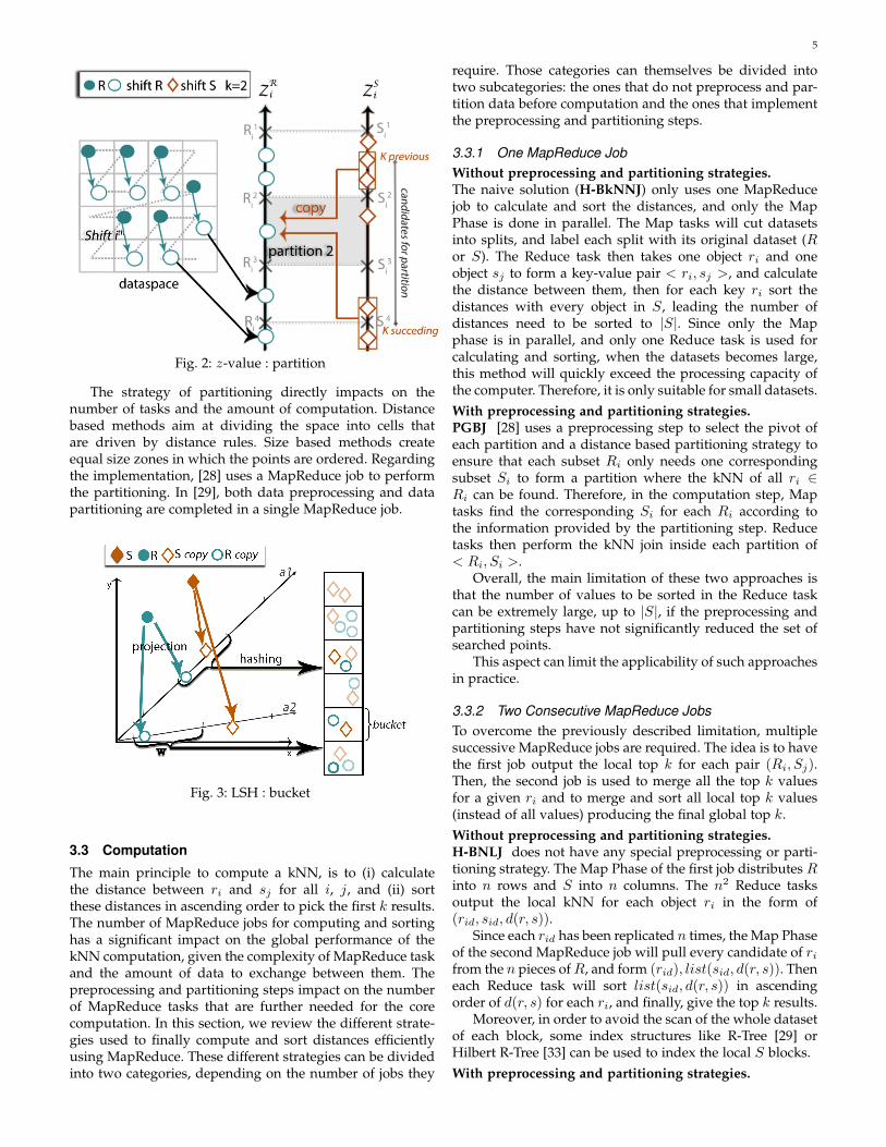
Another type of partitioning strategy aims at dividing datainto equal size partitions. Paper [29] proposes a partitioningstrategy based on z-value described in the previous section.

In order to have a similar number of elements in all npartitions, the authors first sample the dataset and computethe n quantiles. These quantiles are an unbiased estimationof the bounds for each partition. Figure 2 shows an examplefor this method. In this example data are only shifted once.Then, data are projected using z-value method, and theinterpolating “Z” in the figure indicates the neighborhoodafter projection. Data is projected into a one dimensionspace, represented by ZR

i and ZSi in the figure. ZR

i isdivided into partitions using the sampling estimation ex-plained above. For a given partition Ri, its correspondingSi is defined in ZS

i by copying the nearest k preceding andthe nearest k succeeding points to the boundaries of Si. InFigure 2, four points of Si are copied in partition 2, becausethey are considered as candidates for the query points inR2

i .This method is likely to produce a substantially equiv-

alent number of objects in each partition, thus naturallyachieving load balancing. However, the quality of the resultdepends solely on the quality of the z-curve, which mightbe an issue for high dimension data.

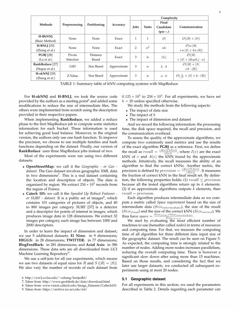
Another similar size based partitioning method usesLocality Sensitive Hashing to first project data into lowdimension space as illustrated in Figure 3. In this example,data is hashed twice using two hash families a1 and a2. Eachhashed data is then projected in the corresponding bucket.The principle of this method is to result in collisions for datathat is spatially close. So the data initially close in the highdimension space is hashed to the same bucket with a highprobability, provided that the bucket size (parameter W inLSH) is large enough to receive at least one copy of closedata.

5

Fig. 2: z-value : partition

The strategy of partitioning directly impacts on thenumber of tasks and the amount of computation. Distancebased methods aim at dividing the space into cells thatare driven by distance rules. Size based methods createequal size zones in which the points are ordered. Regardingthe implementation, [28] uses a MapReduce job to performthe partitioning. In [29], both data preprocessing and datapartitioning are completed in a single MapReduce job.

Fig. 3: LSH : bucket

3.3 Computation

The main principle to compute a kNN, is to (i) calculatethe distance between ri and sj for all i, j, and (ii) sortthese distances in ascending order to pick the first k results.The number of MapReduce jobs for computing and sortinghas a significant impact on the global performance of thekNN computation, given the complexity of MapReduce taskand the amount of data to exchange between them. Thepreprocessing and partitioning steps impact on the numberof MapReduce tasks that are further needed for the corecomputation. In this section, we review the different strate-gies used to finally compute and sort distances efficientlyusing MapReduce. These different strategies can be dividedinto two categories, depending on the number of jobs they

require. Those categories can themselves be divided intotwo subcategories: the ones that do not preprocess and par-tition data before computation and the ones that implementthe preprocessing and partitioning steps.

3.3.1 One MapReduce JobWithout preprocessing and partitioning strategies.The naive solution (H-BkNNJ) only uses one MapReducejob to calculate and sort the distances, and only the MapPhase is done in parallel. The Map tasks will cut datasetsinto splits, and label each split with its original dataset (Ror S). The Reduce task then takes one object ri and oneobject sj to form a key-value pair < ri, sj >, and calculatethe distance between them, then for each key ri sort thedistances with every object in S, leading the number ofdistances need to be sorted to |S|. Since only the Mapphase is in parallel, and only one Reduce task is used forcalculating and sorting, when the datasets becomes large,this method will quickly exceed the processing capacity ofthe computer. Therefore, it is only suitable for small datasets.With preprocessing and partitioning strategies.PGBJ [28] uses a preprocessing step to select the pivot ofeach partition and a distance based partitioning strategy toensure that each subset Ri only needs one correspondingsubset Si to form a partition where the kNN of all ri ∈Ri can be found. Therefore, in the computation step, Maptasks find the corresponding Si for each Ri according tothe information provided by the partitioning step. Reducetasks then perform the kNN join inside each partition of< Ri, Si >.

Overall, the main limitation of these two approaches isthat the number of values to be sorted in the Reduce taskcan be extremely large, up to |S|, if the preprocessing andpartitioning steps have not significantly reduced the set ofsearched points.

This aspect can limit the applicability of such approachesin practice.

3.3.2 Two Consecutive MapReduce JobsTo overcome the previously described limitation, multiplesuccessive MapReduce jobs are required. The idea is to havethe first job output the local top k for each pair (Ri, Sj).Then, the second job is used to merge all the top k valuesfor a given ri and to merge and sort all local top k values(instead of all values) producing the final global top k.Without preprocessing and partitioning strategies.H-BNLJ does not have any special preprocessing or parti-tioning strategy. The Map Phase of the first job distributes Rinto n rows and S into n columns. The n2 Reduce tasksoutput the local kNN for each object ri in the form of(rid, sid, d(r, s)).

Since each rid has been replicated n times, the Map Phaseof the second MapReduce job will pull every candidate of rifrom the n pieces ofR, and form (rid), list(sid, d(r, s)). Theneach Reduce task will sort list(sid, d(r, s)) in ascendingorder of d(r, s) for each ri, and finally, give the top k results.

Moreover, in order to avoid the scan of the whole datasetof each block, some index structures like R-Tree [29] orHilbert R-Tree [33] can be used to index the local S blocks.With preprocessing and partitioning strategies.

6

In H-zkNNJ [29] the authors propose to define the boundsof the partitions of R and then to determine from this thecorresponding Si in a preprocessing job. So here, the pre-processing and partitioning steps are completely integratedin MapReduce. Then, a second MapReduce job takes thepartitions Ri and Si previously determined, and computesfor all ri the candidate neighbor set, which represents thepoints that could be in the final kNN3. To get this candidateneighbor set, the closest k points are taken from eitherside of the considered point (the partition is in dimension1), which leads to exactly 2k candidate points. The thirdMapReduce round determines the exact result for each rifrom the candidate neighbor set. So in total, this solutionuses three MapReduce jobs, and among them, the last twoare actually devoted to the kNN core computation. Asthe number of points that are in the candidate neighborset is small (thanks to the drastic partitioning, itself dueto a drastic preprocessing), the cost of computation andcommunication is extremely reduced.

In RankReduce [27]4, the authors first preprocess datato reduce the dimentionality and partition data into bucketsusing LSH. In our implementation, like in H-zkNNJ, oneMapReduce job is used to calculate the local kNN for eachri, and a second one is used to find the global ones.

3.4 SummarySo far, we have studied the different ways to go through akNN computation from a workflow point of view with threemain steps. The first step focuses on data preprocessing,either for selecting dominating points or for projecting datafrom high dimension to low dimension. The second stepaims at partitioning and organizing data such that thefollowing kNN core computation step is lighten. This laststep can use one or two MapReduce jobs depending on thenumber of distances we want to calculate and sort. Figure 4summarizes the workflow we have gone through in thissection and the techniques associated with each step.

4 THEORETICAL ANALYSIS

4.1 Load BalanceIn a MapReduce job, the Map tasks or the Reduce tasks willbe processed in parallel, so the overall computation time ofeach phase depends on the completion time of the longesttask. Therefore, in order to obtain the best performance, itis important that each task performs substantially the sameamount of computation. When considering load balancingin this section, we mainly want to have the same time com-plexity in each task. Ideally, we want to calculate roughlythe same number of distance between ri and sj in each task.

For H-BkNNJ, there is no load balancing problem. Be-cause in this basic method, only the Map Phase is treatedin parallel. In Hadoop each task will process 64M data bydefault.

H-BNLJ cuts both the dataset R and the dataset S intop equal-size pieces, then those pieces are combined pairwise

3. Note that the notion of candidate points is different from local topk points.

4. Although RankReduce only computes kNN for a single query, it isdirectly expandable to a full kNN join.

to form a partition of < Ri, Sj >. Each task will process oneblock of data so we need to ensure that the size of the datablock handled by each task is roughly the same. However,H-BNLJ uses a random partitioning method which can notexactly divide the data into equal-size blocks.

PGBJ uses Voronoi diagram to cut the data space of Rinto cells, where each cell is represented by its pivot. Thenthe data are assigned to the cell whose pivot is the nearestfrom it. For each R cell, we need to find the correspondingpieces of data in S. Sometimes, the data in S may bepotentially needed by more than oneR cells, which will leadto the duplication of some elements of S. Thus the numberof distances to be calculated in each task, i.e. the relativetime complexity of each task is:

O (Task) =∣∣PR

i

∣∣× (∣∣PSi

∣∣+ |RepSc|)

where∣∣PR

i

∣∣ and∣∣PS

i

∣∣ represents the number of elementsin cell PR

i or PSi respectively, and |RepSc| the number of

replicated elements for the cell. Therefore, to ensure loadbalancing, we need to ensure that O (Task) is roughly thesame for each task. PGBJ introduces two methods to groupthe cells together to form a bigger cell which is the inputof a task. On one hand, the geo grouping method supposesthat close cells have a higher probability to replicate thesame data. On the other hand, the greedy grouping methodestimates the cells whose data are more likely to be repli-cated. This approximation gives an upper bound on thecomplexity of the computation for a particular cell, whichenables grouping of the cells that have the most replicateddata in common. This leads to a minimization of replicationand leads to groups that generate the same workload.

And the H-zkNNJ method assumes:∀ i 6= j,

if |Ri| = |Rj | or |Si| = |Sj |,then |Ri| × |Si| ≈ |Rj | × |Sj |

That is to say, if the number of objects in each partition ofR is equivalent, then the sum of the number of k nearestneighbors of all objects in each partition can be consideredapproximately equivalent, and vice versa. So an efficientpartitioning should try to enforce either (i) |Ri| = |Rj | or(ii) |Si| = |Sj |. In paper [29], the authors give a short proofwhich shows that the worst-case computational complexityfor (i) is equal to:

O (|Ri| × log |Si|) = O( |R|n× log |S|

)(3)

and for choice (ii), the worst-case complexity is equal to:

O (|Ri| × log |Si|) = O(|R| × log |S|

n

)(4)

where n is the number of partitions. Since n � |S|, theoptimal partitioning is achieved when |Ri| = |Rj |.

In RankReduce, a custom partitioner is used to loadbalance tasks between reducers. Let Wh =| Rh | × | Sh | bethe weight of bucket h. A bin packing algorithm is used suchthat each reducer ends up with approximately the sameamount of work. More precisely, let O (Ri) =

∑hWh the

work done by reducerRi, then this methods guarantees that

∀i 6= j,O (Ri) ≈ O (Rj) (5)

7

Fig. 4: Usual workflow of a kNN computation using MapReduce

Because the weight of a bucket is only an approximationof the computing time, this method can only give an ap-proximate load balance. Having a large number of bucketscompared to the number of reducers significantly improvesthe load balancing.

4.2 Accuracy

Usually, the lack of accuracy is the direct consequence oftechniques to reduce the dimensionality with techniquessuch as z-values and LSH. In [29] (H-zkNNJ), the authorsshow that when the dimension of the data increases, thequality of the results tends to decrease. This can be counter-balanced by increasing the number of random shifts appliedto the data, thereby increasing the size of the resultingdataset. Their experiments show that three shifts of the ini-tial dataset (in dimension 15) are sufficient to achieve a goodapproximation (less than 10% of errors measured), whilecontrolling the computation time. Furthermore, paper [34]shows a detailed theoretical analyses showing that, for anyfixed dimension, by using only O(1) random shifts of data,the z-value method returns a constant factor approximationin terms of the radius of the k nearest neighbor ball.

For LSH, the accuracy is defined by the probability thatthe method will return the real nearest neighbor. Supposethat the points within a distance d = |p− q| are consideredas close points. The probability [35] that these two pointsend up in the same bucket is:

p(d) = PrH [h(p) = h(q)] =

∫ W

0

1

dfs(

x

d)(1− x

W)dx (6)

where W is the size of the bucket and fs is the probabilitydensity function of the hash function H. From this equationwe can see that for a given bucket size W, this probability de-creases as the distance d increases. Another way to improvethe accuracy of LSH is to increase the number of hashingfamilies used. The use of LSH in RankReduce has an inter-esting consequence on the number of results. Depending onthe parameters, the number of elements in a bucket mightbe smaller than k. Overall, unlike z-value, the performanceof LSH depends a lot on parameter tuning.

4.3 Global Complexity

Carefully balancing the number of jobs, tasks, computa-tion and communication is an important part of designingan efficient distributed algorithm. All the kNN algorithmsstudied in this survey have different characteristics. We willnow describe them and outline how they can impact theexecution time.(1) The number of MapReduce jobs: Starting a job

(whether in Hadoop [36] or any other platform) re-quires some initialization steps such as allocating re-sources and copying data. Those steps can be very timeconsuming.

(2) The number of Map tasks and Reduce tasks used tocalculate kNN(Ri n S): The larger this number is, themore information is exchanged through the networkduring the shuffle phase. Moreover, scheduling a taskalso incurs an overhead. But the smaller this number is,the more computation is done by one machine.

(3) The number of final candidates for each object ri:We have seen that advanced algorithms use pre-processing and partitioning techniques to reduce thisnumber as much as possible. The goal is to reduce theamount of data transmitted and the computational cost.

Together these three points impact two main overheadsthat affect the performance:• Communication overhead, which can be considered

as the amount of data transmitted over the networkduring the shuffle phases.

• Computation overhead, which is mainly composed oftwo parts: 1). computing the distances, 2). finding the ksmallest distances. It is also impacted by the complexity(dimension) of the data.

Suppose the dataset is d dimensional, the overhead forcomputing the distance is roughly the same for every ri andsj for each method. The difference comes from the numberof distances to sort for each element ri to get the top knearest neighbors. Suppose that the dataset R is dividedinto n splits. Here n represents the number of partitions ofR and S for H-BNLJ and H-zkNNJ, the number of cellsafter using the grouping strategy for PGBJ and the numberof buckets for RankReduce. Assuming there is a good load

8

balance for each method, the number of elements in one splitRi can be considered as |R|n . Finding the k closest neighborsefficiently for a given ri can be done using a priority queue,which less costly than sorting all candidates.

Since all these algorithms uses different strategies, theirsteps cannot be directly compared. Nonetheless, to providea theoretical insight, we will now compare their complexityfor the last phase, which is common to all of them.

The basic method H-BkNNJ only uses one MapRe-duce job, and requires only one Reduce task to computeand sort the distances. The communication overhead isO(|R| + |S|). The number of final candidates for one riis |S|. The complexity of finding the k smallest distancesfor ri is O(|S| · log (k)). Hence, the total cost for one task isO(|R|·|S|·log (k)). Since R and S are usually large datasets,this method quickly becomes impracticable.

To overcome this limitation, H-BNLJ [29] uses twoMapReduce jobs, with n2 tasks to compute the distances.Using a second job significantly reduces the number offinal candidates to nk. The total communication overheadis O(n |R|+n |S|+ kn |R|). The complexity of finding the kelements for each ri is reduced to (n · k) · log (k). Since eachtask has |R|n elements, the total sort overhead for one task isO(|R| · k · log(k)).

PGBJ [28] performs a preprocessing phase followed bytwo MapReduce jobs. This method also only uses n Maptasks to compute the distances and the number of finalcandidates falls to |Si|. Since this method uses a distancebased partitioning method, the size of |Si| varies, dependingon the number of cells required to perform the computationand the number of replications (|RepSc|, see Section 4.1)required by each cell. As such, the computational com-plexity cannot be expressed easily.Overall, finding the kelements is reduced to O(|Si| · log |k|) for each ri, andO( |R|n · |Si| · log |Si|) in total per task. The communicationoverhead is O(|R|+ |S|+ |RepSc| ·n). In the original paperthe authors gives a formula to compute |RepSc| · n, whichis the total number of replications for the whole dataset S.

In RankReduce [27], the initial dataset is projected by Lhash families into buckets. After finding the local candidatesin the second job, the third job combines the local results tofind the global k nearest neighbor. For each ri, the numberof final candidates is L · k. Finding the k elements takesO(L · k · log(k)) per ri, and O(|Ri| · L · k · log(k)) per task.The total communication cost becomesO(|R|+ |S|+k · |R|).

H-zkNNJ [29] also begins by a preprocessing phaseand uses in total three MapReduce jobs in exchange forrequiring only n Map tasks. For a given ri, these tasksprocess elements from the candidate neighbor set C (ri).By construction, C (ri) only contains α · k neighbors,where α is the number of shifts of the original dataset.The complexity is now reduced to O((α · k) · log (k)) forone ri, and O( |R|n · (α · k) · log (k)) in total per task. Thecommunication overhead is O( 1

ε2 + |S| + k · |R|), withε ∈ (0, 1), a parameter of the sampling process.

From the above analysis we can infer the following. H-BkNNJ only uses one task, but this task needs to calculatethe entire data set. H-BNLJ uses n2 tasks to greatly reducethe amount of data processed by each task. However this

also increases the amount of data to be exchanged amongthe nodes. This should prove to be a major bottleneck.PGBJ, RankReduce and H-zkNNJ all use three jobs whichreduces the number of tasks to n, and thus reduces thecommunication overhead.

Although the computational complexity of each task de-pends on various parameters of the preprocessing phases, itis possible to outline a partial conclusion from this analysis.There are basically three performance brackets. First, theleast efficient should be H-BkNNJ, followed by H-BNLJ.PGBJ, RankReduce and H-zkNNJ are theoretically the mostefficient. Among them, PGBJ has the largest number of finalcandidates. For RankReduce and H-zkNNJ , the numberof final candidates is of the same order of magnitude.The main difference lies in the communication complexity,more precisely in 1

ε2 compared to |R|. As the dataset sizeincreases, we will have eventually |R| � 1

ε2 . Hence, H-zkNNJ seems to be the theoretically most efficient for largequery sets.

4.4 Wrap upAlthough the workflow for computing kNN on MapReduceis the same for all existing solutions, the guarantees offeredby each of them vary a lot. As load balancing is a key pointto reduce completion time, one should carefully choose thepartitioning method to achieve this goal. Also, the accuracyof the computing system is crucial: are exact results reallyneeded? If not, then one might trade accuracy for efficiency,by using data transformation techniques before the actualcomputation. Complexity of the global system should alsobe taken into account for particular needs, although it isoften related to the accuracy: an exact system is usuallymore complex than an approximate one. Table 1 shows asummary of the systems we have examined and their maincharacteristics.

Due to the multiple parameters and very different stepsfor each algorithm, we had to limit our complexity analysisto common operations. Moreover, for some of them, thecomplexity depends on parameters set by a user or someproperties of the dataset. Therefore, the total processing timemight be different, in practice, than the one predicted by thetheoretical analysis. That is why it is important to have athorough experimental study.

5 EVALUATION

In order to compare theoretical performance and perfor-mance in practice, we performed an extensive experimen-tal evaluation of the algorithms described in the previoussections.

The experiments were run on two clusters of Grid’50005,one with Opteron 2218 processors and 8GB of memory, theother with Xeon E5520 processors and 32GB of memory,using Hadoop 1.3, 1Gb/s Ethernet and SATA hard drives.We follow the default configuration of Hadoop: (1) thenumber of replications for each split of data is set to 3; (2) thenumber of slot of each node is 1, so only one map/reducetask is processed on the node at one time.

We evaluate the five approaches presented before.

5. www.grid5000.fr

9

Methods Preprocessing Partitioning Accuracy

Complexity

Jobs TasksFinal

Candidate(per ri)

Communication

H-BkNNJ(Basic Method)

None None Exact 1 1 |S| O(|R|+ |S|)

H-BNLJ [29](Zhang et al.)

None None Exact 2 n2 nkO(n |R|

+n |S|+ kn |R|)PGBJ [28](Lu et al.)

PivotsSelection

DistanceBased

Exact 3 n |Si|O(|R|

+ |S|+ |RepSc| · n)RankReduce [27]

(Stupar et al.)LSH Size Based Approximate 3 n L · k

O(|R|+ |S|+k · |R|)

H-zkNNJ [29](Zhang et al.)

Z-Value Size Based Approximate 3 n α · k O( 1ε2

+ |S|+ k · |R|)

TABLE 1: Summary table of kNN computing systems with MapReduce

For H-zkNNJ and H-BNLJ, we took the source codeprovided by the authors as a starting point6 and added somemodifications to reduce the size of intermediate files. Theothers were implemented from scratch using the descriptionprovided in their respective papers.

When implementing RankReduce, we added a reducephase to the first MapReduce job to compute some statisticsinformation for each bucket. These information is usedfor achieving good load balance. Moreover, in the originalversion, the authors only use one hash function. To improvethe precision, we choose to use multiple families and hashfunctions depending on the dataset. Finally, our version ofRankReduce uses three MapReduce jobs instead of two.

Most of the experiments were ran using two differentdatasets:

• OpenStreetMap: we call it the Geographic - or Geo -dataset. The Geo dataset involves geographic XML datain two dimensions7. This is a real dataset containingthe location and description of objects. The data isorganized by region. We extract 256 ∗ 105 records fromthe region of France.

• Catech 101: we call it the Speeded Up Robust Features -or SURF - dataset. It is a public set of images8, whichcontains 101 categories of pictures of objects, and 40to 800 images per category. SURF [37] is a detectorand a descriptor for points of interest in images, whichproduces image data in 128 dimensions. We extract 32images per category, each image has between 1000 and2000 descriptors.

In order to learn the impact of dimension and dataset,we use 5 additional datasets: El Nino: in 9 dimensions;HIGGS: in 28 dimensions; TWITTER: in 77 dimensions;BlogFeedBack: in 281 dimensions; and Axial Axis: in 386dimensions. These data sets are all downloaded from UCIMachine Learning Repository9.

We use a self-join for all our experiments, which meanswe use two datasets of equal sizes for R and S (|R| = |S|).We also vary the number of records of each dataset from

6. http://ww2.cs.fsu.edu/∼czhang/knnjedbt/7. Taken from: http://www.geofabrik.de/data/download.html8. Taken from: www.vision.caltech.edu/Image Datasets/Caltech1019. Taken from: https://archive.ics.uci.edu/ml/

0.125 ∗ 105 to 256 ∗ 105. For all experiments, we have setk = 20 unless specified otherwise.

We study the methods from the following aspects:• The impact of data size• The impact of k• The impact of dimension and datasetAnd we record the following information: the processing

time, the disk space required, the recall and precision, andthe communication overhead.

To assess the quality of the approximate algorithms, wecompute two commonly used metrics and use the resultsof the exact algorithm PGBJ as a reference. First, we definethe recall as recall = |A(v)

⋂I(v)|

|I(v)| , where I(v) are the exactkNN of v and A(v) the kNN found by the approximatemethods. Intuitively, the recall measures the ability of analgorithm to find the correct kNNs. Another metric, theprecision is defined by precision = |A(v)

⋂I(v)|

|A(v)| . It measuresthe fraction of correct kNN in the final result set. By defini-tion, the following properties holds: (1) recall ≤ precisionbecause all the tested algorithms return up to k elements.(2) if an approximate algorithms outputs k elements, thenrecall = precision.

Each algorithm produces intermediate data so we com-pute a metric called Space requirement based on the size ofintermediate data (Sizeintermediate), the size of the result(Sizefinal) and the size of the correct kNN (Sizecorrect). Wethus have space = Sizefinal+Sizeintermediate

Sizecorrect.

We start by evaluating the most efficient number ofmachines to use (hereafter called nodes) in terms of resourcesand computing time. For that, we measure the computingtime of all algorithm for three different data input size ofthe geographic dataset. The result can be seen on Figure 5.As expected, the computing time is strongly related to thenumber of nodes. Adding more nodes increases parallelism,reducing the overall computing time. There is however asignificant slow down after using more than 15 machines.Based on those results, and considering the fact that welater use larger datasets, we conducted all subsequent ex-periments using at most 20 nodes.

5.1 Geographic datasetFor all experiments in this section, we used the parametersdescribed in Table 2. Details regarding each parameter can

10

2 4 6 8 10 12 14 16 18Number of nodes

0

5

10

15

20

Tim

e (

min

)

4∗103 records

H-zkNNJ RankReduce PGBJ H-BNLJ H-BkNNJ

2 4 6 8 10 12 14 16 18Number of nodes

0

20

40

60

80

100

120

140200∗103 records

2 4 6 8 10 12 14 16 18Number of nodes

20

40

60

80

100

120

1404000∗103 records

Fig. 5: Impact of the number of nodes on computing time

be found in sections 3.1 and 3.2. For RankReduce, the valueof W was adapted to get the best performance from eachdataset. For datasets up to 16 ∗ 105 records, W = 32 ∗ 105,up to 25∗105 records,W = 25∗105 and finally,W = 15∗105for the rest of the experiments.

Algorithm Partitioning Reducers ConfigurationH-BNLJ 10 partitions 100 reducers

PGBJ 3000 pivots 25 reducersk-means+ greedy

RankReduce W =

32 ∗ 105

25 ∗ 105

15 ∗ 10525 reducers

L = 2M = 7

H-zkNNJ 10 partitions 30 reducers 3 shifts, p=10

TABLE 2: Algorithm parameters for geographic dataset

5.1.1 Impact of input data size

Our first set of experiments measures the impact of thedata size on execution time, disk space and recall. Figure 6ashows the global computing time of all algorithms, varyingthe number of records from 0.125 ∗ 105 to 256 ∗ 105. Theglobal computing time increases more or less exponen-tially for all algorithms, but only H-zkNNJ and RankRe-duce can process medium to large datasets. For smalldatasets, PGBJ can compute an exact solution as fast as theother algorithms.

Figure 6b shows the space requirement of each algorithmas a function of the final output size. To reduce the footprintof each run, intermediate data are compressed. For example,for H-BNLJ, the size of intermediate data is 2.6 times biggerthan the size of output data. Overall, the algorithms withthe lowest space requirements are RankReduce and PGBJ.

Figure 6c shows the recall and precision of the twoapproximate algorithms, H-zkNNJ and RankReduce. SinceH-zkNNJ always return k elements, its precision and recallare identical. As the number of records increases, its recalldecreases, while still being high, because of the space fillingcurves used in the preprocessing phase. On the other hand,the recall of RankReduce is always lower than its precisionbecause it outputs less than k elements. It benefits fromlarger datasets because more data end up in the samebucket, increasing the number of candidates. Overall, thequality of RankReduce was found to be better than H-zkNNJ on the Geo dataset.

5.1.2 Impact of kChanging the value of k can have a significant impacton the performance of some of the kNN algorithms. Weexperimented on a dataset of 2 ∗ 105 records (only 5 ∗ 104for H-BNLJ for performance reasons) with values for kvarying from 2 to 512. Results are shown in Figure 7 usinga logarithmic scale on the x-axis.

First, we observe a global increase in computing time(Figure 7a) which matches the complexity analysis per-formed earlier. As k increases, the performance of H-zkNNJ,compared to the other advanced algorithms, decreases. Thisis due to the necessary replication of the z-values of Sthroughout the partitions to find enough candidates: thecore computation is thus much more complex.

Second, the algorithms can also be distinguished con-sidering their disk usage, visible on Figure 7b. The globaltendency is that the ratio of intermediate data size over thefinal data size decreases. This means that for each algorithmthe final data size grows faster than the intermediate datasize. As a consequence, there is no particular algorithm thatsuffers from such a bottleneck at this point. PGBJ is themost efficient from this aspect. Its replication of data occursindependently of the number of selected neighbors. Thus,increasing k has a small impact on this algorithm, both incomputing time and space requirements. On this figure, aninteresting observation can also be made for H-zkNNJ. Fork = 2, it has by far the largest disk usage but becomessimilar to the others for larger values. This is because H-zkNNJ creates a lot of intermediate data (copies of theinitial dataset, vectors for the space filling curve, sampling...)irrespective of the value of k. As k increases, so does theoutput size, mitigating the impact of these intermediatedata.

Surprisingly, changing k has a different impact on therecall of the approximate kNN methods, as can be seenon Figure 7c. For RankReduce, increasing k has a negativeimpact on the recall which sharply decreases when k ≥ 64.This is because the window parameter (W ) of LSH wasset at the beginning of the experiments to achieve the bestperformance for this particular dataset. However, it wasnot modified for various of k. Thus it became less optimalas k increased. This shows there is a link between globalparameters such as k and parameters of the LSH process.When using H-zkNNJ, increasing k improves the precision:the probability to have incorrect points is reduced as thereare more candidates in a single partition.

5.1.3 Communication OverheadOur last set of experiments looks at inter-node communica-tion by measuring the amount of data transmitted duringthe shuffle phase (Figure 8). The goal is to compare thesemeasurements with the theoretical analysis in Section 4.3,

Impact of data size. For Geo dataset (Figure 8a), H-BNLJ has indeed a lot of communication. For a dataset of1 ∗ 105 records, the shuffle phase transmits almost 4 timesthe original size. Both RankReduce and H-zkNNJ have aconstant factor of 1 because of the duplication of the originaldataset to improve the recall. The most efficient algorithm isPGBJ for two reasons. First it does not duplicate the originaldataset and second, it relies on various grouping strategiesto minimize replication.

11

0.120.25 0.5 1 2 4 8 16 32 64 128 256Number of records ( ∗105 )

50

100

150

200

Tim

e(m

in)

H-zkNNJ

RankReduce

PGBJ

H-BNLJ

H-BkNNJ

(a) Time

0.120.25 0.5 1 2 4 8 16 32 64 128 256Number of records ( ∗105 )

0

1

2

3

4

Space

requir

em

ent

H-zkNNJ

RankReduce

PGBJ

H-BNLJ

H-BkNNJ

3

6

9

12

resu

lt s

ize (

GB

)

(b) Result size and Disk Usage

0.12 0.25 0.5 1 2Number of records ( ∗105 )

0.80

0.85

0.90

0.95

1.00

Reca

ll &

Pre

cisi

on

H-zkNNJ

RankReduce

recall

precision

(c) Recall and Precision

Fig. 6: Geo dataset impact of the data set size

2 8 32 64 128 256 512k

10

20

30

40

50

Tim

e (

min

)

H-zkNNJ

RankReduce

PGBJ

H-BNLJ

(a) Time

2 8 32 64 128 256 512k

2

4

6

8

Space

requir

em

ent

H-zkNNJ

RankReduce

PGBJ

H-BNLJ

0.6

1.2

1.8

2.4

Resu

lt s

ize (

GB

)

(b) Result size and Disk Usage

2 8 32 64 128 256 512k

0.5

0.6

0.7

0.8

0.9

1.0

Reca

ll &

Pre

cisi

on

H-zkNNJ

RankReduce

recall precision

(c) Recall and Precision

Fig. 7: Geo dataset with 200k records (50k for H-BNLJ), impact of K

0.120.25 0.5 1 2 4 8 16 32 64 128 256Number of records ( ∗105 )

2

4

6

Com

munic

ati

on o

verh

ead r

ati

o

H-zkNNJ

RankReduce

PGBJ

H-BNLJ

2

4

6

8

|R|+

|S|

(GB

)

(a) Impact of the data set size

2 8 32 64 128 256 512k

0

10

20

30

40

50

60

Com

munic

ati

on o

verh

ead r

ati

o

H-zkNNJ

RankReduce

PGBJ

H-BNLJ

(b) Impact of K with 2 ∗ 105 records (0.5 ∗ 105 for H-BNLJ)

Fig. 8: Geo dataset, communication overhead

12

Impact of k. We have performed another set of experi-ments, with a fixed dataset of 2 ∗ 105 records (only 0.5 ∗ 105for H-BNLJ). The results can be seen in Figure 8b. Fordifferent values of k, we have a similar hierarchy thanwith the data size. For RankReduce and H-zkNNJ, theshuffle increases linearly because the number of candidatesin the second phase depends on k. Moreover H-zkNNJ alsoreplicates k previous and succeeding elements in the firstphase, and because of that, its overhead becomes significantfor large k. Finally in PGBJ, k has no impact on the shufflephase.

5.2 Image Feature Descriptors (SURF) datasetWe now investigate whether the dimension of input datahas an impact on the kNN algorithms using the SURFdataset. We used the Euclidian distance between descriptorsto measure image similarity. For all experiments in thissection, the parameters mentioned in Table 3 are used.

Algorithm Partitioning Reducers ConfigurationH-BNLJ 10 partitions 100 reducers

PGBJ 3000 pivots 25 reducersk-means

+ geo

RankReduce W = 107 25 reducersL = 5M = 7

H-zkNNJ 6 partitions 30 reducers 5 shifts

TABLE 3: Algorithm parameters for SURF dataset

5.2.1 Impact of input data sizeResults of experiments when varying the number of descrip-tors are shown in Figure 9 using a log scale on the x-axis.We omitted H-BkNNJ as it could not process the data inreasonable time. In Figure 9a, we can see that the executiontime of the algorithms follows globally the same trend aswith the Geo dataset, except for PGBJ. It is a computationalintensive algorithm because the replication process impliescalculating a lot of Euclidian distances. When in dimension128, this part tends to dominate the overall computationtime. Regarding disk usage (Figure 9b), H-zkNNJ is veryhigh because we had to increase the number of shiftedcopies from 3 to 5 to improve the recall. Indeed, compared tothe Geo dataset, it is very low (Figure 9c). Moreover, as thenumber of descriptors increases, H-zkNNJ goes from 30% to15% recall. As explained before, the precision was found tobe equal to the recall, which means the algorithm alwaysreturned k results. This, together with the improvementusing more shifts, proves that the space filling curves usingin H-zkNNJ are less efficient with high dimension data.

5.2.2 Impact of kFigure 10 shows the impact of different values of k onthe algorithms using a logarithmic scale on the x-axis.Again, since for H-BNLJ and H-zkNNJ, the complexity ofthe sorting phase is dependent on k, we can observe acorresponding increase of the execution time (Figure 10a).For RankReduce, the time varies a lot depending on k.This is because of the stochastic nature of the projectionused in LSH. It can lead to buckets containing differentnumber of elements, creating a load imbalance and some

values of k naturally lead to a better load balancing. PGBJ isvery dependent on the value of k because of the groupingphase. Neighboring cells are added until there are enoughelements to eventually identify the k nearest neighbors. Asa consequence, a large k will lead to larger group of cellsand increase the computing time.

Figure 10b shows the effect of k on disk usage. H-zkNNJ starts with a very high ratio of 74 (not showed onthe Figure) and quickly reduces to more acceptable values.RankReduce also experiences a similar pattern to a lesserextend. As opposed to the Geo dataset, SURF descriptorscannot be efficiently compressed, leading to large interme-diate files.

Finally, Figure 10c shows the effect of k on the recall. As kincreases, the recall and precision of RankReduce decreasesfor the same reason as with the Geo dataset. Also, for large k,the recall becomes lower than the precision because we getless than k results. The precision of H-zkNNJ decreases buteventually shows an upward trend. The increased numberof requested neighbors increases the number of precedingand succeeding points copied, slightly improving the recall.

5.2.3 Communication OverheadWith the SURF dataset, we get a very different behaviorthan with the Geo dataset. The shuffle phase of PGBJ is verycostly (Figure 11a). This is an indication of large replicationsincurred by the large dimension of the data and a poorchoice of pivots. When they are too close to each other, entirecells have to be replicated during the grouping phase.

For RankReduce the shuffle is decreased but stay im-portant, essentially because of the replication factor of 5.Finally, the shifts of original data in H-zkNNJ lead to a largecommunication overhead.

Considering now k, we have the same behavior weobserved with the Geo dataset. The only difference isPGBJ which now exhibits a large communication overhead(Figure 11b). This is again because of the choice of pivotsand the grouping of the cells. However, this overhead re-mains constant, irrespective of k.

5.3 Impact of Dimension and Dataset

We now analyze the behavior of these algorithms accordingto the dimension of data. Since some algorithms are datasetdependent (i.e the spatial distribution of data has an impacton the outcome), we need to separate data distributionfrom the dimension. Hence, we use two different kindsof datasets for these experiments. First, we use real worlddata of various dimensions10. Second, we have built spe-cific datasets by generating uniformly distributed data tolimit the impact of clustering. All the experiments wereperformed using 0.5 ∗ 105 records and k = 20.

Since H-BNLJ relies on the dot product, it is not datasetdependent and its execution time increases with the dimen-sion as seen on Figures 12a and 13a.

PGBJ is heavily dependent on data distribution and onthe choice of pivots to build clusters of equivalent size whichimproves parallelism. The comparison of execution timesfor the datasets 128-sift and 281-blog in Figure 12a shows

10. archive.ics.uci.edu/ml/datasets.html

13

0.12 0.25 0.5 1 2 4 8Number of descriptors (*105 )

30

60

90

120

150

Tim

e (

min

)

H-zkNNJ

RankReduce

PGBJ

H-BNLJ

(a) Time

0.12 0.25 0.5 1 2 4 8Number of descriptors (*105 )

2

4

6

8

Space

requir

em

ent

H-zkNNJ

RankReduce

PGBJ

H-BNLJ

0.2

0.4

0.6

0.8

Resu

lt s

ize (

GB

)

(b) Result size and Disk Usage

0.12 0.25 0.5 1Number of descriptors (*105 )

0.1

0.3

0.5

Reca

ll &

Pre

cisi

on

H-zkNNJ

RankReduce

recall

precision

(c) Recall and Precision

Fig. 9: Surf, impact of the dataset size

2 8 32 64 128 256 512k

0

30

60

90

120

Tim

e (

min

)

H-zkNNJ

RankReduce

PGBJ

H-BNLJ

(a) Time

2 8 32 64 128 256 512k

2

5

10

15

20

Space

requir

em

ent

H-zkNNJ

RankReduce

PGBJ

H-BNLJ

0.4

0.8

1.2

1.6

resu

lt s

ize (

GB

)

(b) Result size and Disk Usage

2 8 32 64 128 256 512k

0.2

0.4

0.6

0.8

1.0

Reca

ll &

Pre

cisi

on

H-zkNNJ

RankReduce

recall

precision

(c) Recall and Precision

Fig. 10: Surf dataset with 50k records, impact of K ,

0.12 0.25 0.5 1 2 4 8Number of descriptors (*105 )

1

2

3

4

Com

munic

ati

on O

verh

ead r

ati

o

H-zkNNJ

RankReduce

PGBJ

H-BNLJ

0.5

1.5

2.5

|R|+

|S|

(GB

)

(a) Surf, impact of the dataset size

2 8 32 64 128 256 512k

0

3

6

9

Com

munic

ati

on o

verh

ead r

ati

o

H-zkNNJ

RankReduce

PGBJ

H-BNLJ

(b) Surf dataset with 50k records, impact of K,

Fig. 11: Communication overhead for the Surf dataset

14

2-osm 9-elninos 28-higgs 77-twitter 128-surf 281-blog386-axial-axis

Dimension-File

20

40

60

80

Tim

e(m

in)

H-zkNNJ

RankReduce

PGBJ-Geo Grouping

H-BNLJ

(a) Execution time

2-osm 9-elninos 28-higgs 77-twitter 128-surf 281-blog386-axial-axis

Dimension-File

0.2

0.4

0.6

0.8

1.0

Reca

ll &

Pre

cisi

on

RankReduce

H-zkNNJ

recall

precision

(b) Recall and Precision

Fig. 12: Real datasets of various dimensions

2 9 28 77 128 281 386

Dimension

15

30

45

60

Tim

e(m

in)

H-zkNNJ

RankReduce

PGBJ-Geo Grouping

H-BNLJ

(a) Execution time

2 9 28 77 128 281 386

Dimension0.5

0.6

0.7

0.8

0.9

1.0

Reca

ll &

Pre

cisi

on

RankReduce

H-zkNNJ

recall

precision

(b) Recall and Precision

Fig. 13: Generated datasets of various dimensions

that, although the dimension of data increases, the executiontime is greatly reduced. Nonetheless, the clustering phaseof the algorithm performs a lot of dot product operationswhich makes it dependent on the dimension, as can be seenin Figure 13a.

H-zkNNJ is an algorithm that depends on spatial dimen-sion. Very efficient for low dimension, its execution timeincreases with the dimension (Figure 13a). A closer analysisshows that all phases see their execution time increase.However, the overall time is dominated by the first phase(generation of shifted copies and partitioning) whose timecomplexity sharply increases with dimension. Data distribu-tion has an impact on the recall which gets much lower thanthe precision for some datasets (Figure 12b). With generateddataset (Figure 13b), both recall and precision are identicaland initially very high. However as dimension increases, therecall decreases because of the projection.

Finally, RankReduce is both dependent on the dimen-sion and distribution of data. Experiments with the realdatasets have proved to be difficult because of the variousparameters of the algorithm to obtain the requested numberof neighbors without dramatically increasing the executiontime (see discussion in Section 5.4.5). Despite our efforts, the

precision was very low for some datasets, in particular 28-higgs. Using the generated datasets, we see that its executiontime increases with the dimension (Figure 13a) but its recallremains stable (Figure 13b).

5.4 Practical AnalysisIn this section, we analyze the algorithms from a practicalpoint of view, outlying their sensitivity to the dataset, theenvironment or some internal parameters.

5.4.1 H-BkNNJThe main drawback of H-BkNNJ is that only the Mapphase is in parallel. In addition, the optimal parallelizationis subtle to achieve because the optimal number of nodesto use is defined by input size

input split size . This algorithm is clearlynot suitable for large datasets but because of its simplicity, itcan, nonetheless, be used when the amount of data is small.

5.4.2 H-BNLJIn H-BNLJ, both the Map and Reduce phases are in parallel,but the optimal number of tasks is difficult to find. Given anumber of partitions n, there will be n2 tasks. Intuitively,

15

one would choose a number of tasks that is a multiple ofthe number of processing units. The issue with this strategyis that the distribution of the partitions might be unbal-anced. Figure 14 shows an experiment with 6 partitions and62 = 36 tasks, each executed on a reducer. Some reducerswill have more elements to process than others, slowing thecomputation.

0 5 10 15 20 25 30 35 40Reducer Number

0.4

0.8

1.2

1.6

Num

ber

of

Ele

ments

(∗1

09)

#R*#S

10

20

30

40

Tim

e(m

in)

Fig. 14: H-BNLJ, candidates job, 105 records , 6 partitions,Geo dataset

Overall, the challenge with this algorithm is to find theoptimal number of partitions for a given dataset.

5.4.3 PGBJA difficulty in PGBJ comes from its sampling-based pre-processing techniques because it impacts the partitioningand thus the load balancing. This raises many challenges.First, how to choose the pivots from the initial dataset. Thethree techniques proposed by the authors, farthest, k-meansand random, lead to different pivots and different partitionsand possibly different executions. We found that with ourdatasets, both k-means and random techniques gave thebest performance. Second, the number of pivots is alsoimportant because it will impact the number of partitions.A too small or too large number of pivots will decreaseperformance. Finally, another important parameter is thegrouping strategy used (Section 4.1). In Figure 15, we can see

0.5 1 2 4Number of records ( ∗105 )

0

10

20

30

40

50

60

70

Tim

e (

min

ute

s)

Greedy 50 reducers

Greedy 20 reducers

Geo 20 reducers

0

10

20

30

40

50

60

70

80

90

Gro

upin

g T

ime (

seco

nds)

Fig. 15: PGBJ, overall time (lines) and Grouping time (bars)with Geo dataset, 3000 pivots, KMeans Sampling

that the greedy grouping technique has a higher groupingtime (bars) than the geo grouping technique. However, theglobal computing time (line) using this technique is shorter

thanks to the good load balancing. This is illustrated byFigure 16 which shows the distribution of elements pro-cessed by reducers when using geo grouping (16a) or greedygrouping (16b).

0 5 10 15 20Reducer number

0

20

40

60

80

100

120

140

160

180

Num

ber

of

Ele

ments

(∗1

03)

#S

#R

(a) Geo

0 5 10 15 20Reducer number

0

20

40

60

80

100

120

140

160

180

Num

ber

of

Ele

ments

(∗1

03)

#S

#R

(b) Greedy

Fig. 16: PGBJ, load balancing with 20 reducers

5.4.4 H-zkNNJIn H-zkNNJ, the z-value transformation leads to informa-tion loss. The recall of this algorithm is influenced by thenature, the dimension and the size of the input data. Morespecifically, this algorithm becomes biased if the distancebetween initial data is very scattered, and the more inputdata or the higher the dimension, the more difficult it isto draw the space filling curve. To improve the recall, theauthors propose to create duplicates in the original datasetby shifting data. This greatly increases the amount of data toprocess and has a significant impact on the execution time.

5.4.5 RankReduceRankReduce, with the addition of a third job, can havethe best performance of all, provided that it is started withthe optimal parameters. The most important ones are W ,the size of each bucket, L, the number of hash familiesand M , the number of hash functions in each family. Sincethey are dependent on the dataset, experiments are neededto precisely tune them. In [38], the authors suggests thiscan be achieved with a sample dataset and a theoreticalmodel. The first important metric to consider is the numberof candidates available in each bucket. Indeed, with somepoorly chosen parameter values, it is possible to have lessthan k elements in each bucket, making it impossible tohave enough elements at the end of the computation (thereare less than k neighbors in the result). On the opposite,having too many candidates in each bucket will increasetoo much the execution time. To illustrate the complexity ofthe parameter tuning operation, we have run experimentson the Geo and SURF datasets. First, Figure 17 shows that,for the Geo dataset, increasing W improves the recall andthe precision at the expense of the execution time, up toan optimal before decreasing. This can be explained bylooking at the number of buckets for a given W . As Wincreases, each bucket contains more elements and thustheir number decreases. As a consequence, the probabilityto have the correct k neighbors inside a bucket increases,which improves the recall. However, the computational loadof each bucket also increases.

A similar pattern can be observed with the SURF dataset(Figure 18, left), where increasing W improves the recall

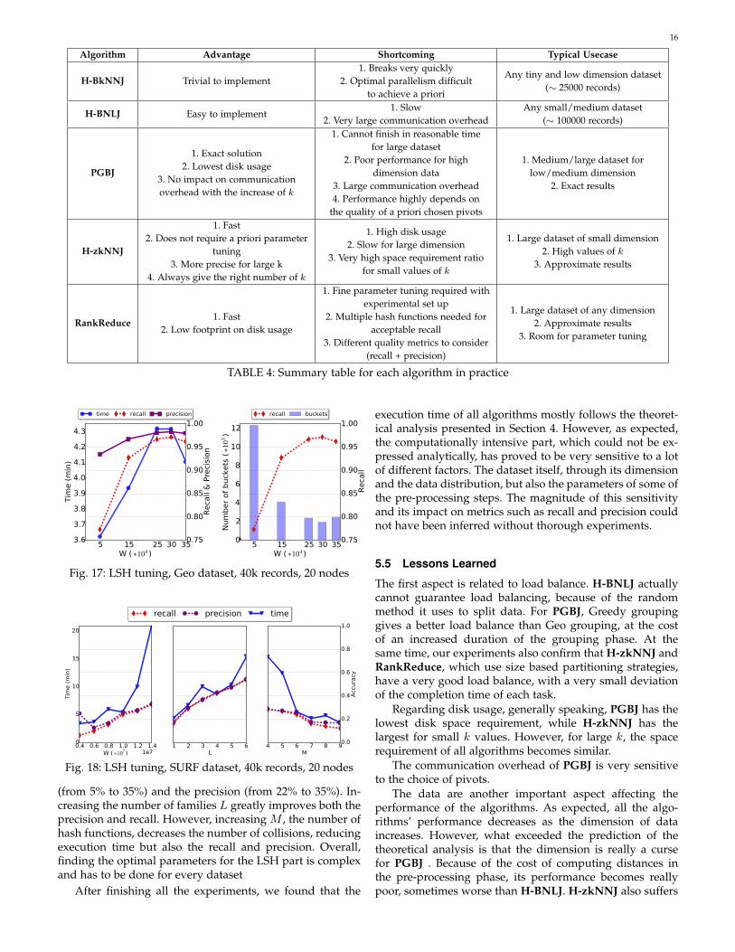
16

Algorithm Advantage Shortcoming Typical Usecase

H-BkNNJ Trivial to implement1. Breaks very quickly

2. Optimal parallelism difficultto achieve a priori

Any tiny and low dimension dataset(∼ 25000 records)

H-BNLJ Easy to implement1. Slow

2. Very large communication overheadAny small/medium dataset

(∼ 100000 records)

PGBJ

1. Exact solution2. Lowest disk usage

3. No impact on communicationoverhead with the increase of k

1. Cannot finish in reasonable timefor large dataset

2. Poor performance for highdimension data

3. Large communication overhead4. Performance highly depends on

the quality of a priori chosen pivots

1. Medium/large dataset forlow/medium dimension

2. Exact results

H-zkNNJ

1. Fast2. Does not require a priori parameter

tuning3. More precise for large k

4. Always give the right number of k

1. High disk usage2. Slow for large dimension

3. Very high space requirement ratiofor small values of k

1. Large dataset of small dimension2. High values of k

3. Approximate results

RankReduce1. Fast

2. Low footprint on disk usage

1. Fine parameter tuning required withexperimental set up

2. Multiple hash functions needed foracceptable recall

3. Different quality metrics to consider(recall + precision)

1. Large dataset of any dimension2. Approximate results

3. Room for parameter tuning

TABLE 4: Summary table for each algorithm in practice

5 15 25 30 35W ( ∗104 )

3.6

3.7

3.8

3.9

4.0

4.1

4.2

4.3

Tim

e (

min

)

time recall precision

0.75

0.80

0.85

0.90

0.95

1.00

Reca

ll &

Pre

cisi

on

5 15 25 30 35W ( ∗104 )

0

2

4

6

8

10

12

Num

ber

of

buck

ets

(∗1

03)

recall buckets

0.75

0.80

0.85

0.90

0.95

1.00

Reca

ll

Fig. 17: LSH tuning, Geo dataset, 40k records, 20 nodes

0.4 0.6 0.8 1.0 1.2 1.4W ( ∗107 ) 1e7

0

5

10

15

20

Tim

e (

min

)

1 2 3 4 5 6L

recall precision time

4 5 6 7 8 9M

0.0

0.2

0.4

0.6

0.8

1.0

Acc

ura

cy

Fig. 18: LSH tuning, SURF dataset, 40k records, 20 nodes

(from 5% to 35%) and the precision (from 22% to 35%). In-creasing the number of families L greatly improves both theprecision and recall. However, increasing M , the number ofhash functions, decreases the number of collisions, reducingexecution time but also the recall and precision. Overall,finding the optimal parameters for the LSH part is complexand has to be done for every dataset

After finishing all the experiments, we found that the

execution time of all algorithms mostly follows the theoret-ical analysis presented in Section 4. However, as expected,the computationally intensive part, which could not be ex-pressed analytically, has proved to be very sensitive to a lotof different factors. The dataset itself, through its dimensionand the data distribution, but also the parameters of some ofthe pre-processing steps. The magnitude of this sensitivityand its impact on metrics such as recall and precision couldnot have been inferred without thorough experiments.

5.5 Lessons Learned

The first aspect is related to load balance. H-BNLJ actuallycannot guarantee load balancing, because of the randommethod it uses to split data. For PGBJ, Greedy groupinggives a better load balance than Geo grouping, at the costof an increased duration of the grouping phase. At thesame time, our experiments also confirm that H-zkNNJ andRankReduce, which use size based partitioning strategies,have a very good load balance, with a very small deviationof the completion time of each task.

Regarding disk usage, generally speaking, PGBJ has thelowest disk space requirement, while H-zkNNJ has thelargest for small k values. However, for large k, the spacerequirement of all algorithms becomes similar.

The communication overhead of PGBJ is very sensitiveto the choice of pivots.

The data are another important aspect affecting theperformance of the algorithms. As expected, all the algo-rithms’ performance decreases as the dimension of dataincreases. However, what exceeded the prediction of thetheoretical analysis is that the dimension is really a cursefor PGBJ . Because of the cost of computing distances inthe pre-processing phase, its performance becomes reallypoor, sometimes worse than H-BNLJ. H-zkNNJ also suffers

17

from the dimension, which decreases its recall. However,the major impact comes from the distribution of data.

In addition, the overall performance is also sensitiveto some specific parameters, especially for RankReduce.Its performance depends a lot on some parameter tuning,which requires extensive experiments.

Based on the experimental results, we summarize theadvantages, disadvantages and suitable usage scenarios foreach algorithm, in Table 4.

6 CONCLUSION

In this paper, we have studied existing solutions to performthe kNN operation in the context of MapReduce. We havefirst approached this problem from a workflow point ofview. We have pointed out that all solutions follow threemain steps to compute kNN over MapReduce, namelypreprocessing of data, partitioning and actual computation.We have listed and explained the different algorithms whichcould be chosen for each step, and developed their pros andcons, in terms of load balancing, accuracy of results, andoverall complexity. In a second part, we have performedextensive experiments to compare the performance, diskusage and accuracy of all these algorithms in the sameenvironment. We have mainly used two real datasets, ageographic coordinates one (2 dimensions) and an imagebased one (SURF descriptors, 128 dimensions). For all algo-rithms, it was the first published experiment on such highdimensions. Moreover, we have performed a fine analysis,outlining, for each algorithm, the importance and difficultyof fine tuning some parameters to obtain the best perfor-mance.

Overall, this work gives a clear and detailed view of thecurrent algorithms for processing kNN on MapReduce. Italso clearly exhibits the limits of each of them in practiceand shows precisely the context where they best perform.Above all, this paper can be seen as a guideline to helpselecting the most appropriate method to perform the kNNjoin operation on MapReduce for a particular use case.

After this thorough analysis, we have found a number oflimitations on existing solution which could be addressedin future work. First, besides H-BkNNJ, all methods needto replicate the original data to some extend. The number ofreplications, although necessary to improve precision, has agreat impact on disk usage and communication overhead.Finding the optimal parameters to reduce this number isstill an open issue. Second, the partitioning methods areall based on properties of R. However, one can expectR to vary as it represents the query set. The cost of re-partitioning is currently prohibitive so, for dynamic queries,better approaches might rely on properties of S. Finally,MapReduce, especially through its Hadoop implementa-tion, is well suited for batch processing of static data. Theefficiency of theses methods on data stream has yet to beinvestigated.

ACKNOWLEDGMENTS

This work was partly funded by the French Government(National Research Agency, ANR) through the Investmentsfor the Future Program reference #ANR-11-LABX-0031-01.

Experiments presented in this paper were carried out usingthe Grid’5000 testbed, supported by a scientific interestgroup hosted by INRIA and including CNRS, RENATERand several Universities as well as other organizations (seehttps://www.grid5000.fr).

REFERENCES

[1] D. Li, Q. Chen, and C.-K. Tang, “Motion-aware knn laplacian forvideo matting,” in ICCV’13, 2013.

[2] H.-P. Kriegel and T. Seidl, “Approximation-based similarity searchfor 3-D surface segments,” Geoinformatica, 1998.

[3] X. Bai, R. Guerraoui, A.-M. Kermarrec, and V. Leroy, “Collabo-rative personalized top-k processing,” ACM Trans. Database Syst.,2011.

[4] D. Rafiei and A. Mendelzon, “Similarity-based queries for timeseries data,” SIGMOD Rec., 1997.

[5] R. Agrawal, C. Faloutsos, and A. N. Swami, “Efficient similaritysearch in sequence databases,” in Foundations of Data Organizationand Algorithms, 1993.

[6] K. Inthajak, C. Duanggate, B. Uyyanonvara, S. Makhanov, andS. Barman, “Medical image blob detection with feature stabilityand knn classification,” in Computer Science and Software Engineer-ing, 2011.

[7] F. Korn, N. Sidiropoulos, C. Faloutsos, E. Siegel, and Z. Protopa-pas, “Fast nearest neighbor search in medical image databases,” inVLDB’96, 1996.

[8] H. V. Jagadish, B. C. Ooi, K.-L. Tan, C. Yu, and R. Zhang, “idis-tance: An adaptive b+-tree based indexing method for nearestneighbor search,” ACM Trans. Database Syst., vol. 30, no. 2, pp.364–397, 2005.

[9] C. Bohm and F. Krebs, “The k-nearest neighbour join: Turbocharging the kdd process,” Knowl. Inf. Syst., vol. 6, no. 6, pp. 728–749, Nov. 2004.

[10] P. Ciaccia, M. Patella, and P. Zezula, “M-tree: An efficient accessmethod for similarity search in metric spaces,” in VLDB’97, 1997.

[11] C. Yu, R. Zhang, Y. Huang, and H. Xiong, “High-dimensional knnjoins with incremental updates,” GeoInformatica, 2010.

[12] J. L. Bentley, “Multidimensional binary search trees used forassociative searching,” Commun. ACM, 1975.

[13] J. Dean and S. Ghemawat, “Mapreduce: Simplified data processingon large clusters,” Commun. ACM, 2008.

[14] G. Song, J. Rochas, F. Huet, and F. Magoules, “Solutions forProcessing K Nearest Neighbor Joins for Massive Data on MapRe-duce,” in 23rd Euromicro International Conference on Parallel, Dis-tributed and Network-based Processing, Turku, Finland, Mar. 2015.

[15] N. Bhatia and A. Vandana, “Survey of nearest neighbor tech-niques,” International Journal of Computer Science and InformationSecurity, 2010.

[16] L. Jiang, Z. Cai, D. Wang, and S. Jiang, “Survey of improving k-nearest-neighbor for classification,” in Fuzzy Systems and Knowl-edge Discovery, 2007.

[17] H. V. Jagadish, B. C. Ooi, K.-L. Tan, C. Yu, and R. Zhang, “idis-tance: An adaptive b+-tree based indexing method for nearestneighbor search,” ACM Trans. Database Syst., 2005.

[18] C. Bohm and F. Krebs, “The k-nearest neighbour join: Turbocharging the kdd process,” Knowl. Inf. Syst., 2004.

[19] C. Yu, R. Zhang, Y. Huang, and H. Xiong, “High-dimensional knnjoins with incremental updates,” Geoinformatica, 2010.

[20] M. I. Andreica and N. T. pus, “Sequential and mapreduce-basedalgorithms for constructing an in-place multidimensional quad-tree index for answering fixed-radius nearest neighbor queries,”2013.

[21] C. Ji, T. Dong, Y. Li, Y. Shen, K. Li, W. Qiu, W. Qu,and M. Guo, “Inverted grid-based knn query processing withmapreduce,” in Proceedings of the 2012 Seventh Grid AnnualConference, ser. CHINAGRID ’12. Washington, DC, USA:IEEE Computer Society, 2012, pp. 25–32. [Online]. Available:http://dx.doi.org/10.1109/ChinaGrid.2012.19

[22] A. Gionis, P. Indyk, and R. Motwani, “Similarity search in highdimensions via hashing,” in VLDB’99, 1999.

[23] B. Yao, F. Li, and P. Kumar, “K nearest neighbor queries andknn-joins in large relational databases (almost) for free,” in DataEngineering, 2010.

18

[24] A. S. Arefin, C. Riveros, R. Berretta, and P. Moscato, “Gpu-fs-knn:A software tool for fast and scalable knn computation using gpus,”PLOS ONE, 2012.

[25] D. Novak and P. Zezula, “M-chord: A scalable distributed similar-ity search structure,” in Scalable Information Systems, 2006.

[26] P. Haghani, S. Michel, and K. Aberer, “Lsh at large distributedknn search in high dimensions ,” in WebDB’08, 2008.

[27] A. Stupar, S. Michel, and R. Schenkel, “Rankreduce - processingk-nearest neighbor queries on top of mapreduce,” in In LSDS-IR,2010.

[28] W. Lu, Y. Shen, S. Chen, and B. C. Ooi, “Efficient processing ofk nearest neighbor joins using mapreduce,” Proc. VLDB Endow.,2012.

[29] C. Zhang, F. Li, and J. Jestes, “Efficient parallel knn joins for largedata in mapreduce,” in Extending Database Technology, 2012.

[30] M. Datar, N. Immorlica, P. Indyk, and V. S. Mirrokni, “Locality-sensitive hashing scheme based on p-stable distributions,” inSymposium on Computational Geometry, 2004.

[31] G. Song, Z. Meng, F. Huet, F. Magoules, L. Yu, and X. Lin, “Ahadoop mapreduce performance prediction method,” in HPCC’13,2013.

[32] X. Zhou, D. J. Abel, and D. Truffet, “Data partitioning for parallelspatial join processing,” Geoinformatica, 1998.

[33] Q. Du and X. Li, “A novel knn join algorithms based on hilbertr-tree in mapreduce,” in Computer Science and Network Technology(ICCSNT), 2013 3rd International Conference on, 2013, pp. 417–420.

[34] B. Yao, F. Li, and P. Kumar, “K nearest neighbor queries andknn-joins in large relational databases (almost) for free,” in DataEngineering (ICDE), 2010 IEEE 26th International Conference on,March 2010, pp. 4–15.

[35] M. Slaney and M. Casey, “Locality-sensitive hashing for find-ing nearest neighbors [lecture notes],” Signal Processing Magazine,IEEE, vol. 25, no. 2, pp. 128–131, March 2008.

[36] D. Jiang, B. C. Ooi, L. Shi, and S. Wu, “The performance ofmapreduce: An in-depth study,” Proc. VLDB Endow., 2010.

[37] H. Bay, T. Tuytelaars, and L. Van Gool, “Surf: Speeded up robustfeatures,” in ECCV’06, 2006.

[38] W. Dong, Z. Wang, W. Josephson, M. Charikar, and K. Li, “Mod-eling lsh for performance tuning,” in Proceedings of the 17th ACMConference on Information and Knowledge Management, ser. CIKM ’08,New York, NY, USA, 2008, pp. 669–678.

Ge Song Ge Song received the B.Sc. degree inApplied Mathematics and the M.Sc. degree inEngineering Sciences from Beihang University,China, in 2010 and 2013 respectively. She iscurrently a Ph.D. candidate in the Departmentof Mathematics and Computer Science at Cen-traleSupelec, Universite Paris-Saclay, France.Her research interests include data mining, bigdata processing, parallel computing and real-time processing.

Justine Rochas Justine Rochas is a computerscience Ph.D. candidate at University Of NiceSophia Antipolis. Her research interests includeprogramming languages, programming modelsand middlewares for parallel and distributedcomputing.

Lea El Beze Lea El Beze was born in Nice,France, in 1992 and acquired Israeli citizenshipin 2013. She received a M.S. degree in computerscience and Big Data from the University of NiceSophia Antipolis, in 2015. She is now working onMiddleware for Big Data in the private sector.http://lea-elbeze.alwaysdata.net/

Fabrice Huet Fabrice Huet holds a M.Sc. inDistributed System and a Ph.D. in ComputerSciences from the University of Nice Sophia An-tipolis. He is currently an Associate Professor atthe Computer Science department of the Univer-sity Nice Sophia Antipolis. His research interestsinclude high performance distributed computing,peer-to-peer architectures and distributed pro-cessing of data streams.

Frederic Magoules Frederic Magoules receivedthe B.Sc. degree in engineering sciences, theM.Sc. degree in applied mathematics, the M.Sc.degree in numerical analysis, and the Ph.D.degree in applied mathematics from UniversitePierre & Marie Curie, France, in 1993, 1994,1995, and 2000, respectively. He is currently aProfessor in the Department of Mathematics andin the Department of Computer Science at Cen-traleSupelec, Universite Paris-Saclay, France.His research interests include parallel computing

and data mining. Prof. Magoules is a Fellow of IMA, a Fellow of BCS, amember of ACM, a member of SIAM and a member of IEEE.