k-Nearest neighbor density estimation on Riemannian

Manifolds.

Guillermo Henry1, Andres Munoz2 and Daniela Rodriguez11Facultad de Ciencias Exactas y Naturales, Universidad de Buenos Aires and CONICET, Argentina.

2 Universidad Tecnologica Nacional and CBC, Universidad de Buenos Aires.

Abstract

In this paper, we consider a k-nearest neighbor kernel type estimator when therandom variables belong in a Riemannian manifolds. We study asymptotic propertiessuch as the consistency and the asymptotic distribution. A simulation study is alsoconsider to evaluate the performance of the proposal. Finally, to illustrate the potentialapplications of the proposed estimator, we analyzed two real example where two differentmanifolds are considered.

Key words and phrases: Asymptotic results, Density estimation, Meteorological applica-tions, Nonparametric, Palaeomagnetic data, Riemannian manifolds.

1 Introduction

Let X1, . . . , Xn be independent and identically distributed random variables taking valuesin IRd and having density function f . A class of estimators of f which has been widelystudied since the work of Rosenblatt (1956) and Parzen (1962) has the form

fn(x) =1

nhd

n∑j=1

K

(x−Xj

h

),

where K(u) is a bounded density on IRd and h is a sequence of positive number such thath→ 0 and nhd →∞ as n→∞.

If we apply this estimator to data coming from long tailed distributions, with a smallenough h to appropriate for the central part of the distribution, a spurious noise appearsin the tails. With a large value of h for correctly handling the tails, we can not see thedetails occurring in the main part of the distribution. To overcome these defects, adaptivekernel estimators were introduced. For instance, a conceptually similar estimator of f(x)was studied by Wagner (1975) who defined a general neighbor density estimators by

fn(x) =1

nHdn(x)

n∑j=1

K

(x−Xj

Hn(x)

),

1

arX

iv:1

106.

4763

v1 [

mat

h.ST

] 2

3 Ju

n 20

11

where Hn(x) is the distance between x and the k-nearest neighbor of x among X1, . . . , Xn,and k = kn is a sequence of non–random integers such that limn→∞ kn =∞. Through theseadaptive bandwidth , the estimation in the point x has the guarantee that to be calculatedusing at least k points of the sample.

However, in many applications, the variables X take values on different spaces thanIRd. Usually these spaces have a more complicated geometry than the Euclidean space andthis has to be taken into account in the analysis of the data. For example if we study thedistribution of the stars with luminosity in a given range it is naturally to think that thevariables belong to a spherical cylinder (S2 × IR) instead of IR4. If we considerer a regionof the planet M , then the direction and the velocity of the wind in this region are pointsin the tangent bundle of M , that is a manifold of dimension 4. Other examples could befound in image analysis, mechanics, geology and other fields. They include distributionson spheres, Lie groups, among others, see for example Joshi, et.at. (2007), Goh and Vidal(2008). For this reason, it is interesting to study an estimation procedure of the densityfunction that take into account a more complex structure of the variables.

Nonparametric kernel methods for estimating densities of spherical data have been stud-ied by Hall, et .al (1987) and Bai, et. al. (1988). Pelletier (2005) proposed a family of non-parametric estimators for the density function based on kernel weight when the variablesare random object valued in a closed Riemannian manifold. The Pelletier’s estimators isconsistent with the kernel density estimators in the Euclidean case considered by Rosenblatt(1956) and Parzen (1962).

As we comment above, the importance of local adaptive bandwidth is well known innonparametric statistics and this is even more true with data taking values on complexityspace. In this paper, we propose a k-nearest neighbor method when the data takes valueson a Riemannian manifolds. The proposal combine the ideas of smoothing in Euclideanspaces with the estimators introduced in Pelletier (2005).

This paper is organized as follows. Section 2 contains a brief summary of the neces-saries concepts of Riemannian geometry. In Section 2.1, we introduce a k-nearest neighborestimators on Riemannian manifolds. Uniform consistency of the estimators is derived inSection 3.1, while in Section 3.2 the asymptotic distribution is obtained under regular as-sumptions. Section 4 contains a Monte Carlo study designed to evaluate the proposedestimators. Finally, Section 5 presents two example using real data. Proofs are given in theAppendix.

2 Preliminaries and the estimator

Let (M, g) be a d−dimensional Riemannian manifold without boundary. We denote by dgthe distance induced by the metric g. With Bs(p) we denote a normal ball with radius scentered at p. The injectivity radius of (M, g) is given by injgM = inf

p∈Msup{s ∈ IR > 0 :

Bs(p) is a normal ball}. Is easy to see that a compact Riemannian manifold has strictlypositive injectivity radius. For example, it is not difficult to see that the d-dimensional

2

sphere Sd endowed with the metric induced by the canonical metric g0 of Rd+1 has injec-tivity radius equal to π. If N is a proper submanifold of the same dimension than (M, g),then injg|NN = 0. The Euclidean space or the hyperbolic space have infinity injectivityradius. Moreover, a complete and simply connected Riemannian manifold with non positivesectional curvature has also this property.

Throughout this paper, we will assume that (M, g) is a complete Riemannian manifold,i.e. (M,dg) is a complete metric space. Also we will consider that injgM is strictly positive.This restriction will be clear in the Section 2.1 when we define the estimator. For standardresult on differential and Riemannian geometry we refer to the reader to Boothby (1975),Besse (1978), Do Carmo (1988) and Gallot, Hulin and Lafontaine (2004).

Let p ∈ M , we denote with 0p and TpM the null tangent vector and the tangent spaceof M at p. Let Bs(p) be a normal ball centered at p. Then Bs(0p) = exp−1p (Bs(p)) is anopen neighborhood of 0p in TpM and so it has a natural structure of differential manifold.We are going to consider the Riemannian metrics g ′ and g ′ ′ in Bs(0p), where g ′ = exp∗p(g)is the pullback of g by the exponential map and g ′ ′ is the canonical metric induced by gpin Bs(0p). Let w ∈ Bs(0p), and (U , ψ) be a chart of Bs(0p) such that w ∈ U . We noteby {∂/∂ψ1|w, . . . , ∂/∂ψd|w} the tangent vectors induced by (U , ψ). Consider the matricialfunction with entries (i, j) are given by g ′

((∂/∂ψi|w

),(∂/∂ψj |w

)). The volumes of the

parallelepiped spanned by {(∂/∂ψ1|w

), . . . ,

(∂/∂ψd|w

)} with respect to the metrics g ′ and

g ′ ′ are given by |det g ′((∂/∂ψi|w

),(∂/∂ψj |w

))|1/2 and |det g ′ ′

((∂/∂ψi|w

),(∂/∂ψj |w

))|1/2

respectively. The quotient between these two volumes is independent of the selected chart.So, given q ∈ Bs(p), if w = exp−1p (q) ∈ Bs(0p) we can define the volume density function,θp(q), on (M, g) as

θp(q) =| det g ′

((∂/∂ψi|w

),(∂/∂ψj |w

))|1/2

|det g ′ ′((∂/∂ψi|w

),(∂/∂ψj |w

))|1/2

for any chart (U , ψ) of Bs(0p) that contains w = exp−1p (q). For instance, if we consider anormal coordinate system (U,ψ) induced by an orthonormal basis {v1, . . . , vd} of TpM thenθp(q) is the function of the volume element dνg in the local expression with respect to chart(U,ψ) evaluated at q, i.e.

θp(q) =

∣∣∣∣∣det gq

(∂

∂ψi

∣∣∣q,∂

∂ψj

∣∣∣q

)∣∣∣∣∣12

,

where ∂∂ψi|q = Dαi(0)expp(αi(0)) with αi(t) = exp−1p (q) + tvi for q ∈ U . Note that the

volume density function θp(q) is not defined for all the pairs p and q in M , but it is ifdg(p, q) < injgM .

We finish the section showing some examples of the density function:

i) In the case of (IRd, g0) the density function is θp(q) = 1 for all (p, q) ∈ IRd × IRd.

ii) In the 2-dimensional sphere of radius R, the volume density is

θp1(p2) = R|sen(dg(p1, p2)/R)|

dg(p1, p2)if p2 6= p1,−p1 and θp1(p1) = 1.

3

where dg induced is given by

dg(p1, p2) = R arccos(< p1, p2 >

R2).

iii) In the case of the cylinder of radius 1 C1 endowed with the metric induced by thecanonical metric of IR3, θp1(p2) = 1 for all (p1, p2) ∈C1×C1, and the distance inducedis given by dg(p1, p2) = d2((r1, s1), (r2, s2)) if d2((r1, s1), (r2, s2)) < π, where d2 is theEuclidean distance of IR2 and pi = (cos(ri), sin(ri), si) for i = 1, 2.

See also, Besse (1978) and Pennec (2006) for a discussion on the volume density function.

2.1 The estimator

Consider a probability distribution with a density f on a d−dimensional Riemannian man-ifold (M, g). Let X1, · · · , Xn be i.i.d random object takes values on M with density f . Anatural extension of the estimator proposed by Wagner (1975) in the context of a Rieman-nian manifold is to consider the following estimator

fn(p) =1

nHdn(p)

n∑j=1

1

θXj (p)K

(dg(p,Xj)

Hn(p)

),

where K : IR → IR is a non-negative function with compact support, θp(q) denotes thevolume density function on (M, g) and Hn(p) is the distance dg between p and the k-nearest neighbor of p among X1, . . . , Xn, and k = kn is a sequence of non–random integerssuch that limn→∞ kn =∞.

As we mention above, the volume density function is not defined for all p and q. There-fore, in order to guarantee the well definition of the estimator we consider a modification ofthe proposed estimator. Using the fact that the kernel K has compact support, we consideras bandwidth ζn(p) = min{Hn(p), injgM} instead of Hn(p). Thus, the kernel only consi-ders the points Xi such that dg(Xi, p) ≤ ζn(p) that are smaller than injgM and for thesepoints, the volume density function is well defined. Hence, the k-nearest neighbor kerneltype estimator is defined as follows,

fn(p) =1

nζdn(p)

n∑j=1

1

θXj (p)K

(dg(p,Xj)

ζn(p)

), (1)

where ζn(p) = min{Hn(p), injgM}.Remark 2.1.1. If (M, g) is a compact Riemannian manifold and its sectional curvatureis not bigger than a > 0, then we know by the Lemma of Klingerberg (see Gallot, Hulin,Lafontaine (2004)) that injgM ≥ min{π/

√a, l/2} where l is the length of the shortest

closed geodesic in (M, g).

4

3 Asymptotic results

Denote by C`(U) the set of ` times continuously differentiable functions from U to IR whereU is an open set of M . We assume that the measure induced by the probability P and byX is absolutely continuous with respect to the Riemannian volume measure dνg, and wedenote by f its density on M with respect to dνg. More precisely, let B(M) be the Borelσ−field of M (the σ−field generated by the class of open sets of M). The random variableX has a probability density function f , i.e. if χ ∈ B(M), P (X−1(χ)) =

∫χ fdνg.

3.1 Uniform Consistency

We will consider the following set of assumptions in order to derive the strong consistencyresults of the estimate fn(p) defined in (1).

H1. Let M0 be a compact set on M such that:

i) f is a bounded function such that infp∈M0 f(p) = A > 0.

ii) infp,q∈M0 θp(q) = B > 0.

H2. For any open set U0 of M0 such that M0 ⊂ U0, f is of class C2 on U0.

H3. The sequence kn is such that kn →∞, knn → 0 and kn

logn →∞ as n→∞.

H4. K : IR→ IR is a bounded nonnegative Lipschitz function of order one, with compactsupport [0, 1] satisfying:

∫IRd K(‖u‖)du = 1,

∫IRd uK(‖u‖)du = 0 and

0 <∫IRd ‖u‖2K(‖u‖)du <∞.

H5. The kernel K(u) verifies K(uz) ≥ K(z) for all u ∈ (0, 1).

Remark 3.1.1. The fact that θp(p) = 1 for all p ∈ M guarantees that H1 ii) holds.The assumption H3 is usual when dealing with nearest neighbor and the assumption H4 isstandard when dealing with kernel estimators.

Theorem 3.1.2. Assume that H1 to H5 holds, then we have that

supp∈M0

|fn(p)− f(p)| a.s.−→ 0.

3.2 Asymptotic normality

To derive the asymptotic distribution of the regression parameter estimates we will needtwo additional assumptions. We will denote with Vr the Euclidean ball of radius r centeredat the origin and with λ(Vr) its Lebesgue measure.

H5. f(p) > 0, f ∈ C2(V ) with V ⊂ M an open neighborhood of M and the secondderivative of f is bounded.

5

H6. The sequence kn is such that kn →∞, kn/n→ 0 as n→∞ and there exists 0 ≤ β <∞such that

√knn−4/(d+4) → β as n→∞.

H7. The kernel verifies

i)∫K1(‖u‖)‖u‖2du <∞ as s→∞ where K1(u) = K ′(‖u‖)‖u‖.

ii) ‖u‖d+1K2(u)→ 0 as ‖u‖ → ∞ where K2(u) = K ′′(‖u‖)‖u‖2 −K1(u)

Remark 3.2.1. Note that div(K(‖u‖)u) = K ′(‖u‖)‖u‖ + d K(‖u‖), then using thedivergence Theorem, we get that

∫K ′(‖u‖)‖u‖du =

∫‖u‖=1K(‖u‖)u u

‖u‖du−d∫K(‖u‖)du.

Thus, the fact that K has compact support in [0, 1] implies that∫K1(u)du = −d.

On the other hand, note that ∇(K(‖u‖)‖u‖2) = K1(‖u‖)u + 2K(‖u‖)u and by H4 weget that

∫K1(‖u‖)udu = 0.

Theorem 3.2.2. Assume H4 to H7. Then we have that√kn(fn(p)− f(p))

D−→ N (b(p), σ2(p))

with

b(p) =1

2

βd+4d

(f(p)λ(V1))2d

∫V1K(‖u‖)u21 du

d∑i=1

∂f ◦ ψ−1

∂ui∂ui|u=0

and

σ2(p) = λ(V1)f2(p)∫V1K2(‖u‖)du

where u = (u1, . . . , ud) and (Bh(p), ψ) is any normal coordinate system.

In order to derive the asymptotic distribution of fn(p), we will study the asymptoticbehavior of hdn/ζ

dn(p) where hdn = kn/(nf(p)λ(V1)). Note that if we consider fn(p) =

kn/(nζdn(p)λ(V1)), fn(p) is a consistent estimator of f(p) (see the proof of Theorem 3.1.2.).

The next Theorem states that this estimator is also asymptotically normally distributed asin the Euclidean case.

Theorem 3.2.3. Assume H4 to H6, and let hdn = kn/(nf(p)λ(V1)). Then we have that

√kn

(hdnζdn(p)

− 1

)D−→ N(b1(p), 1)

with

b1(p) =

(β

d+42

f(p)µ(V1)

) 2d{

τ

6d+ 12+

∫V1 u

21 du L1(p)

f(p)µ(V1)

}where u = (u1, . . . , ud), τ is the scalar curvature of (M, g), i.e. the trace of the Ricci tensor,

L1(p) =d∑i=1

(∂2f ◦ ψ−1

∂uiui

∣∣∣u=0

+∂f ◦ ψ−1

∂ui

∣∣∣u=0

∂θp ◦ ψ−1

∂ui

∣∣∣u=0

)

and (Bh(p), ψ) is any normal coordinate system.

6

4 Simulations

This section contains the results of a simulation study designed to evaluate the performanceof the estimator defined in the Section 2.1. We consider three models in two differentRiemannian manifolds, the sphere and the cylinder endowed with the metric induced bythe canonical metric of IR3. We performed 1000 replications of independent samples of sizen = 200 according to the following models:

Model 1 (in the sphere): The random variables Xi for 1 ≤ i ≤ n are i.i.d. VonMises distribution VM(µ, κ) i.e.

fµ,κ(X) =

(k

2

)1/2

I1/2(κ) exp{κXtµ},

with µ is the mean parameter, κ > 0 is the concentration parameter and I1/2(κ) =(κπ2

)sinh(κ) stands for the modified Bessel function. This model has many important

applications, as described in [16] and [19]. We generate a random sample follows aVon Mises distribution with mean (0, 0, 1) and concentration parameter 3.

Model 2 (in the sphere): We simulate i.i.d. random variables Zi for 1 ≤ i ≤ nfollowing a multivariate normal distribution of dimension 3, with mean (0, 0, 0) andcovariance matrix equals to the identity. We define Xi = Zi

‖Zi‖ for 1 ≤ i ≤ n, thereforethe variables Xi follow an uniform distribution in the two dimensional sphere.

Model 3 (in the cylinder): We consider random variables Xi = (yi, ti) takingvalues in the cylinder S1 × IR. We generated the model proposed by Mardia andSutton (1978) where,

yi = (cos(θi), sin(θi)) ∼ VM((−1, 0), 5)

ti|yi ∼ N(1 + 2√

5 cos(θi), 1).

Some examples of variables with this distribution can be found in Mardia and Sutton(1978).

In all cases, for smoothing procedure, the kernel was taken as the quadratic kernelK(t) = (15/16)(1 − t2)2I(|x| < 1). We have considered a grid of equidistant values of kbetween 5 and 150 of length 20.

To study the performance of the estimators of the density function f , denoted by fn, wehave considered the mean square error (MSE) and the median square error (MedSE), i.e,

MSE(fn) =1

n

n∑i=1

[fn(Xi)− f(Xi)]2 .

MedSE(fn) = median |fn(Xi)− f(Xi)|2 .

7

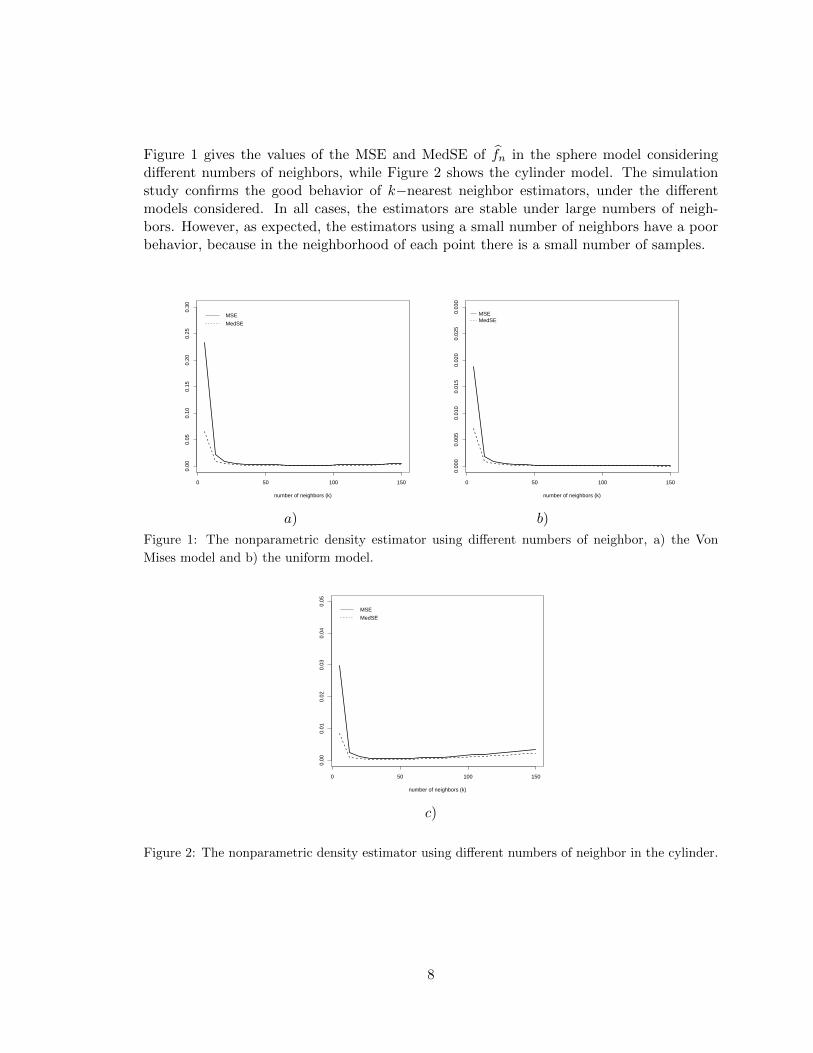
Figure 1 gives the values of the MSE and MedSE of fn in the sphere model consideringdifferent numbers of neighbors, while Figure 2 shows the cylinder model. The simulationstudy confirms the good behavior of k−nearest neighbor estimators, under the differentmodels considered. In all cases, the estimators are stable under large numbers of neigh-bors. However, as expected, the estimators using a small number of neighbors have a poorbehavior, because in the neighborhood of each point there is a small number of samples.

0 50 100 150

0.00

0.05

0.10

0.15

0.20

0.25

0.30

number of neighbors (k)

MSE

MedSE

0 50 100 150

0.00

00.

005

0.01

00.

015

0.02

00.

025

0.03

0

number of neighbors (k)

MSEMedSE

a) b)

Figure 1: The nonparametric density estimator using different numbers of neighbor, a) the Von

Mises model and b) the uniform model.

0 50 100 150

0.00

0.01

0.02

0.03

0.04

0.05

number of neighbors (k)

MSE

MedSE

c)

Figure 2: The nonparametric density estimator using different numbers of neighbor in the cylinder.

8

5 Real Example

5.1 Paleomagnetic data

It is well know the need for statistical analysis of paleomagnetic data. Since the workdeveloped by Fisher (1953), the study of parametric families was considered a principal toolsto analyze and quantify this type of data (see Cox and Doell (1960), Butler (1992) and Loveand Constable (2003)). In particular, our proposal allows to explore the nature of directionaldataset that include paleomagnetic data without make any parametric assumptions.

In order to illustrate the k-nearest neighbor kernel type estimator on the two-dimensionalsphere, we illustrate the estimator using a paleomagnetic data set studied by Fisher, Lewis,and Embleton (1987). The data set consist in n = 107 sites from specimens of Precambrianvolcanos whit measurements of magnetic remanence. The data set contains two variablescorresponding to the directional component on a longitude scale, and the directional com-ponent on a latitude scale. The original data set is available in the library sm of R statisticalpackage.

To calculate the estimators the volume density function and the geodesic distance weretaken as in the Section 2 and we considered the quadratic kernel K(t) = (15/16)(1 −t2)2I(|x| < 1). In order to analyzed the sensitivity of the results with respect to the numberof neighbors, we plot the estimator using different bandwidths. The results are shown inthe Figure 3.

The real data was plotted in blue and with a large radius in order to obtain a bettervisualization. The Equator line, the Greenwich meridian and a second meridian are in graywhile the north and south pols are denoted with the capital letter N and S respectively.The levels of concentration of measurements of magnetic remanence can be found in yellowfor high levels and in red for lowest density levels. Also, the levels of concentration ofmeasurements of magnetic remanence was illustrated with relief on the sphere that allowto emphasize high density levels and the form of the density function.

As in the Euclidean case large number of neighbors produce estimators with smallvariance but high bias, while small values produce more wiggly estimators. This fact showsthe need of the implementation of a method to select the adequate bandwidth for thisestimators. However, this require further careful investigation and are beyond the scope ofthis paper.

9

S

N

S

N

a) b)

S

N

S

N

c) d)

Figure 3: The nonparametric density estimator using different number of neighbors, a) k=75,b)k=50, c) k=25 and d) k=10.

5.2 Meteorological data

In this Section, we consider a real data set collected in the meteorological station “Aguita de Perdiz”that is located in Viedma, province of Rıo Negro, Argentine. The dataset consists in the winddirection and temperature during January 2011 and contains 1326 measurements that were registeredwith a frequency of thirty minutes. We note that the considered variables belong to a cylinder withradius 1.

As in the previous Section, we consider the quadratic kernel and we took the density functionand the geodesic distance as in Section 2. Figure 4 shows the result of the estimators, the color andform of the graphic was constructed as in the previous example.

It is important to remark that the measurement devices of wind direction not present a sufficientprecision to avoid repeated data. Therefore, we consider the proposal given in Garcıa-Portugues,et.al. (2011) to solve this problem. The proposal consists in perturb the repeated data as followsri = ri + ξεi, where ri denote the wind direction measurements and εi, for i = 1, . . . , n wereindependently generated from a von Mises distribution with µ = (1, 0) and κ = 1. The selection ofthe perturbation scale ξ was taken ξ = n−1/5 as in Garcıa-Portugues, et.al. (2011) where in thiscase n = 1326

10

The work of Garcıa-Portugues, et.al. (2011) contains other nice real example where the proposedestimator can be apply. They considered a naive density estimator applied to wind directions andSO2 concentrations, that allow you explore high levels of contamination.

S

45

-5

S

45

-5

N

N

S

45

-5

S

45

-5

N

N

a) b)

S

S

-5

45

-5

45

N

N

S

S

45

-5

-5

45

N

N

c) d)

Figure 4: The nonparametric density estimator using different number of neighbors, a) k=75,b)k=150, c) k=300 and d) k=400.

In Figure 4, we can see that the lowest temperature are more probable when the wind comesfrom the East direction. However, the highest temperature does not seem to have correlation withthe wind direction. Also, note that in Figure 4, we can see two mode corresponding to the minimumand maximum daily of the temperature.

These examples show the usefulness of the proposed estimator for the analysis and explorationof these type of dataset.

Appendix

Proof of Theorem 3.1.2.

Let

fn(p, δn) =1

nδdn

n∑i=1

1

θXi(p)

K

(dg(p,Xi)

δn

).

Note that if δn = δn(p) verifies δ1n ≤ δn(p) ≤ δ2n for all p ∈ M0 where δ1n and δ2n satisfy δin → 0

andnδdinlog n

→∞ as n→∞ for i = 1, 2 then by Theorem 3.2 in Henry and Rodriguez (2009) we have

that

supp∈M0

|fn(p, δn)− f(p)| a.s.−→ 0 (2)

For each 0 < β < 1 we define,

f−n (p, β) =1

nD+n (β)d

n∑i=1

1

θXi(p)K

(dg(p,Xi)

D−n (β)

)= f−n (p,D−n (β)d)

D−n (β)d

D+n (β)d

.

f+n (p, β) =1

nD−n (β)d

n∑i=1

1

θXi(p)K

(dg(p,Xi)

D+n (β)

)= f+n (p,D+

n (β)d)D+n (β)d

D−n (β)d.

where D−n (β) = β1/2dhn, D+n (β) = β−1/2dhn and hdn = kn/(nλ(V1)f(p)) with λ(V1) denote the

Lebesgue measure of the ball in IRd with radius r centered at the origin. Note that

supp∈M0

|f−n (p, β)− βf(p)| a.s.−→ 0 and supp∈M0

|f+n (p, β)− β−1f(p)| a.s.−→ 0. (3)

For all 0 < β < 1 and ε > 0 we define

S−n (β, ε) = {w : supp∈M0

|f−n (p, β)− f(p)| < ε },

S+n (β, ε) = {w : sup

p∈M0

|f+n (p, β)− f(p)| < ε },

Sn(ε) = {w : supp∈M0

|fn(p)− f(p)| < ε },

An(β) = {f−n (p, β) ≤ fn(p) ≤ f+n (p, β)}

Then, An(β) ∩ S−n (β, ε) ∩ S+n (β, ε) ⊂ Sn(ε). Let A = supp∈M0

f(p). For 0 < ε < 3A/2 andβε = 1− ε

3A consider the following sets

Gn(ε) ={w : D−n (βε) ≤ ζn(p) ≤ D+

n (βε) for all p ∈M0

}G−n (ε) = { sup

p∈M0

|f−n (p, βε)− βεf(p)| < ε

3}

G+n (ε) = { sup

p∈M0

|f+n (p, βε)− β−1ε f(p)| < ε

3}.

Then we have that Gn(ε) ⊂ An(βε), G−n (ε) ⊂ S−n (βε, ε) and G+

n (ε) ⊂ S+n (βε, ε). Therefore, Gn(ε)∩

G−n (ε) ∩G+n (ε) ⊂ Sn(ε).

12

On the other hand, using that limr→0 V (Br(p))/rdµ(V1) = 1, where V (Br(p)) denotes the

volume of the geodesic ball centered at p with radius r (see Gray and Vanhecke (1979)) and similararguments those considered in Devroye and Wagner (1977), we get that

supp∈M0

∣∣∣∣ knnλ(V1)f(p)Hd

n(p)− 1

∣∣∣∣ a.s.−→ 0.

Recall that injgM > 0 and Hdn(p)

a.s.−→ 0. Then for straightforward calculations we obtained that

supp∈M0

∣∣∣ knnλ(V1)f(p)ζdn(p)

− 1∣∣∣ a.s.−→ 0. Thus, IGc

n(ε)a.s.−→ 0 and (3) imply that ISc

n(ε)a.s.−→ 0.

Proof of Theorem 3.2.2.

A Taylor expansion of second order gives

√kn

1

nζdn(p)

n∑j=1

1

θXj(p)

K

(dg(p,Xj)

ζn(p)

)− f(p)

= An +Bn + Cn

where

An = (hdn/ζdn(p))

√kn

1

nhdn

n∑j=1

1

θXj (p)K

(dg(p,Xj)

hn

)− f(p)

,

Bn =√kn((hdn/ζ

dn(p))− 1)

f(p) +[(hn/ζn(p))− 1]hdn

[(hdn/ζdn(p))− 1]ζdn(p)

1

nhdn

n∑j=1

1

θXj (p)K1

(dg(p,Xj)

ζn(p)

)and

Cn =√kn((hdn/ζ

dn(p))− 1)

[(hn/ζn(p))− 1]2

2[(hdn/ζdn(p))− 1]

1

nζdn(p)

n∑j=1

1

θXj (p)K2

(dg(p,Xj)

ξn

)[ξn/hn]2

with hdn = kn/nf(p)λ(V1) and min(hn, ζn) ≤ ξn ≤ max(hn, ζn). Note that H6 implies that hnsatisfies the necessary hypothesis given in Theorem 4.1 in Rodriguez and Henry (2009), in particular√

nhd+4n → β

d+4d (f(p)λ(V1))−

d+42d .

By the Theorem and the fact that hn/ζn(p)p−→ 1, we obtain that An converges to a normal

distribution with mean b(p) and variance σ2(p). Therefore it is enough to show that Bn and Cnconverges to zero in probability.

Note that (hn/Hn(p))−1(hd

n/ζdn(p))−1

p−→ d−1 and by similar arguments those considered in Theorem 3.1 in

Pelletier (2005) and Remark 3.2.1. we get that

1

nhdn

n∑j=1

1

θXj (p)K1

(dg(p,Xj)

ζn(p)

)p−→∫K1(u)duf(p) = −d f(p).

Therefore, by Theorem 3.2.3., we obtain that Bnp−→ 0. As ξn/hn converges to one in probability,

in order to concluded the proof, it remains to prove that

1

nζdn(p)

n∑j=1

1

θXj(p)|K2 (dg(p,Xj)/ξn) |

13

is bounded in probability.

By H7, there exits r > 0 such that |t|d+1|K2(t)| ≤ 1 if |t| ≥ r. Let Cr = (−r, r), then we havethat

1

nζdn(p)

n∑j=1

1

θXj (p)

∣∣∣∣K2

(dg(p,Xj)

ξn

)∣∣∣∣ ≤ sup|t|≤r |K2(t)|nζdn(p)

n∑j=1

1

θXj (p)ICr

(dg(p,Xj)

ξn

)

+1

nζdn(p)

n∑j=1

1

θXj(p)

ICcr

(dg(p,Xj)

ξn

) ∣∣∣∣dg(p,Xj)

ξn

∣∣∣∣−(d+1)

As min(hn, ζn(p)) ≤ ξn ≤ max(hn, ζn(p)) = ξn it follows that

1

nζdn(p)

n∑j=1

1

θXj (p)

∣∣∣∣K2

(dg(p,Xj)

ξn

)∣∣∣∣ ≤≤

(hnζn(p)

)dsup|t|≤r|K2(t)| 1

nhdn

n∑j=1

1

θXj(p)

ICr

(dg(p,Xj)

hn

)

+ sup|t|≤r|K2(t)| 1

nζdn(p)

n∑j=1

1

θXj (p)ICr

(dg(p,Xj)

ζn(p)

)

+

(hnζn(p)

)d1

nhdn

n∑j=1

1

θXj (p)ICc

r

(dg(p,Xj)

hn

) ∣∣∣∣dg(p,Xj)

hn

∣∣∣∣−(d+1)∣∣∣∣∣ ξnhn

∣∣∣∣∣(d+1)

+1

nζdn(p)

n∑j=1

1

θXj (p)ICc

r

(dg(p,Xj)

ζn(p)

) ∣∣∣∣dg(p,Xj)

ζn(p)

∣∣∣∣−(d+1)∣∣∣∣∣ ξnζn(p)

∣∣∣∣∣(d+1)

= Cn1 + Cn2 + Cn3 + Cn4.

By similar arguments those considered in Theorem 3.1 in Pelletier (2005), we have that Cn1p−→

f(p)∫ICr

(s)ds and Cn3p−→ f(p)

∫ICc

r(s)|s|−(d+1)ds.

Finally, let Aεn = {(1 − ε)hn ≤ ζn ≤ (1 + ε)hn} for 0 ≤ ε ≤ 1. Then for n large enoughP (Aεn) > 1− ε and in Aεn we have that

ICr

(dg(Xj , p)

ζn(p)

)≤ ICr

(dg(Xj , p)

(1 + ε)hn

),

ICcr

(dg(Xj , p)

ζn(p)

) ∣∣∣∣dg(Xj , p)

ζn(p)

∣∣∣∣−(d+1)

≤ ICcr

(dg(Xj , p)

(1− ε)hn

) ∣∣∣∣ dg(Xj , p)

(1− ε)hn

∣∣∣∣−(d+1) ∣∣∣∣ ζn(p)

(1− ε)hn

∣∣∣∣(d+1)

.

This fact and analogous arguments those considered in Theorem 3.1 in Pelletier (2005), allow toconclude the proof.

Proof of Theorem 3.2.3.

Denote bn = hdn/(1 + zk−1/2n ), then

P (√kn(hdn/ζ

dn − 1) ≤ z) = P (ζdn ≥ bn) = P (Hd

n ≥ bn, injgMd ≥ bn).

As bn → 0 and injgM > 0, there exists n0 such that for all n ≥ n0 we have that

P (Hdn ≥ bn, injgMd ≥ bn) = P (Hd

n ≥ bn).

14

Let Zi such that Zi = 1 when dg(p,Xi) ≤ b1/dn and Zi = 0 elsewhere. Thus, we have that P (Hd

n ≥bn) = P (

∑ni=1 Zi ≤ kn). Let qn = P (dg(p,Xi) ≤ b1/dn ). Note that qn → 0 and nqn →∞ as n→∞,

therefore

P

(n∑i=1

Zi ≤ kn

)= P

(1√nqn

n∑i=1

(Zi − E(Zi)) ≤1√nqn

(kn − nqn)

).

Using the Lindeberg Central Limit Theorem we easily obtain that (nqn)−1/2∑n

i=1(Zi − E(Zi))is asymptotically normal with mean zero and variance one. Hence, it is enough to show that

(nqn)−1/2

(kn − nqn)p−→ z + b1(p).

Denote by µn = n

∫B

b1/dn

(p)

(f(q) − f(p))dνg(q). Note that µn = n qn − wn with wn =

n f(p)V (Bb1/dn

(p)). Thus,

1√nqn

(kn − nqn) = w−1/2n (kn − wn)

(wn

wn + µn

)1/2

+µn

w1/2n

(wn

wn + µn

)1/2

.

Let (Bb1/dn

(p), ψ) be a coordinate normal system. Then, we note that

1

λ(Vb1/dn

)

∫B

b1/dn

(p)

f(q)dνg(q) =1

λ(Vb1/dn

)

∫V

b1/dn

f ◦ ψ−1(u)θp ◦ ψ−1(u)du.

The Lebesgue’s Differentiation Theorem and the fact thatV (B

b1/dn

(p))

λ(Vb1/dn

)→ 1 imply that

λnwn→ 0.

On the other hand, from Gray and Vanhecke (1979), we have that

V (Br(p)) = rdλ(V1)(1− τ

6d+ 12r2 +O(r4)).

Hence, we obtain that

w−1/2n (kn − wn) =w−1/2n kn z k

−1/2n

1 + zk−1/2n

+w−1/2n τb

2/dn kn

(6d+ 12)(1 + zk−1/2n )

+ w−1/2n kn O(b4/dn )

= An +Bn + Cn.

It’s easy to see that An → z and w−1/2n b

2/dn kn =

knn−1/2b2/d−1/2

n

(f(p)λ(V1))−2/d

(bnλ(V1)

V (Bb1/dn

(p))

)1/2

, since H6 we

obtain that Bn → τ β(d+4)/d/(6d+ 12) (f(p)µ(V1))−2/d. A similar argument shows that Cn → 0

and therefore we get that w−1/2n (kn − wn)→ z + β

d+4d

τ6d+12 (f(p)λ(V1))−d/2.

In order to concluded the proof we will show thatµn

w1/2n

→ βd+4d

(f(p)λ(V1))(d+2)/d

∫V1u21 du L1(p).

We use a second Taylor expansion that leads to,∫B

b1/dn

(p)

(f(q)− f(p))dνg(q) =

d∑i=1

∂f ◦ ψ−1

∂ui|u=0b

1+1/dn

∫V1ui θp ◦ ψ−1(b1/dn u) du

+

d∑i,j=1

∂2f ◦ ψ−1

∂ui∂uj|u=0b

1+2/dn

∫V1uiuj θp ◦ ψ−1(b1/dn u) du

+ O(b1+3/dn ).

15

Using again a Taylor expansion on θp ◦ ψ−1(·) at 0 we have that∫B

b1/dn

(p)

(f(q)− f(p))dνg(q) = b1+2/dn

∫V1u21 du L1(p) +O(b1+3/d

n )

and by H6 the theorem follows.

References

[1] Bai, Z.D.; Rao, C. and Zhao, L. (1988). Kernel Estimators of Density Function of DirectionalData. J. Multivariate Anal. 27, 24-39.

[2] Berger, M.; Gauduchon, P. and Mazet, E. (1971). Le Spectre d’ une variete Riemannienne.Springer-Verlag.

[3] Boothby, W. M. (1975). An introduction to differentiable manifolds and Riemannian geometry.Academic Press, New York.

[4] Butler, R. (1992). Paleomagnetism:Magnetic Domains to Geologic Terranes.Blackwell ScientificPublications.

[5] Cox, A. and Doell, R. (1960). Review of Paleomagnetism, Geol. Soc. Amer. Bull. 71, 645768.

[6] Devroye, L., and Wagner, T.J. (1977), ‘The strong uniform consistency of nearest neighbordensity estimates’, Annals of Statistics,3, 536-540.

[7] Do Carmo, M. (1988). Geometria Riemaniana. Proyecto Euclides, IMPA. 2da edicion.

[8] Fisher, R. A. (1953). Dispersion on a sphere. Proc. Roy. Soc. London, Ser. A 217, 295305.

[9] Fisher, N.I., T. Lewis, and B. J. J. Embleton (1987). Statistical Analysis of Spherical Data.New York: Cambridge University Press.

[10] Gallot, S., Hulin, D. and Lafontaine J. (2004) Riemannian Geometry. Spriger. Third Edition.

[11] Garcıa-Portugues, E; Crujeiras, R. and Gonzalez-Manteiga, W. (2011). Exploring wind directionand SO2 concentration by circularlinear density estimation. Prepint.

[12] Goh, A. and Vidal, R. (2008). Unsupervised Riemannian Clustering of Probability DensityFunctions. Lecture Notes In Artificial Intelligence. 5211.

[13] Gray, A. and Vanhecke, L. (1979), ‘Riemannian geometry as determined by the volumes ofsmall geodesic balls’, Acta Math., 142, 157-198.

[14] Hall, P. , Watson, G.S. and Cabrera, J. (1987). Kernel density estimation with spherical data.Biometrika 74, 751762.

[15] Henry, G. and Rodriguez, D. (2009). Kernel Density Estimation on Riemannian Manifolds:Asymptotic Results. Journal Math. Imaging Vis. 43, 235-639.

[16] Jammalamadaka, S. and SenGupta, A. (2001). Topics in Circular Statistics. Multivariate Anal-ysis, 5. World Scientific, Singapore.

[17] Joshi, J., Srivastava, A. and Jermyn, I. H. (2007). Riemannian Analysis of Probability DensityFunctions with Applications in Vision. Proc. IEEE Computer Vision and Pattern Recognition.

[18] Love, J. and Constable, C. (2003). Gaussian statistics for palaeomagnetic vectors. Geophys. J.Int. 152, 515565.

16

[19] Mardia, K., and Jupp, P. (2000). Directional Data, New York: Wiley.

[20] Mardia, K. and Sutton, T. (1978). A Model for Cylindrical Variables with Applications. Journalof the Royal Statistical Society. Series B. (Methodological),40,229-233.

[21] Parzen, E. (1962). On estimation of a probability density function and mode. Ann. Math.Statist. 33, 1065–1076.

[22] Pelletier, B. (2005). Kernel Density Estimation on Riemannian Manifolds. Statistics and Prob-ability Letters, 73, 3, 297-304.

[23] Pennec, X. (2006). Intrinsic Statistics on Riemannian Manifolds: Basic Tools for GeometricMeasurements. Journal Math. Imaging Vis., 25, 127-154.

[24] Rosenblatt, M. (1956). Remarks on some nonparametric estimates of a density function. Ann.Math. Statist.27, 832–837

[25] Wagner, T. (1975). Nonparametric estimates of probability densities. IEEE Trans. InformationTheory IT. 21, 438–440.

17