k-means Requires Exponentially Many Iterations...

Discrete Comput Geom (2011) 45: 596–616DOI 10.1007/s00454-011-9340-1

k-means Requires Exponentially Many IterationsEven in the Plane

Andrea Vattani

Received: 30 June 2009 / Revised: 29 November 2009 / Accepted: 7 December 2009 /Published online: 23 March 2011© The Author(s) 2011. This article is published with open access at Springerlink.com

Abstract The k-means algorithm is a well-known method for partitioning n pointsthat lie in the d-dimensional space into k clusters. Its main features are simplicityand speed in practice. Theoretically, however, the best known upper bound on itsrunning time (i.e., nO(kd)) is, in general, exponential in the number of points (whenkd = Ω(n/ logn)). Recently Arthur and Vassilvitskii (Proceedings of the 22nd An-nual Symposium on Computational Geometry, pp. 144–153, 2006) showed a super-polynomial worst-case analysis, improving the best known lower bound from Ω(n)

to 2Ω(√

n) with a construction in d = Ω(√

n) dimensions. In Arthur and Vassilvitskii(Proceedings of the 22nd Annual Symposium on Computational Geometry, pp. 144–153, 2006), they also conjectured the existence of super-polynomial lower bounds forany d ≥ 2.

Our contribution is twofold: we prove this conjecture and we improve the lowerbound, by presenting a simple construction in the plane that leads to the exponentiallower bound 2Ω(n).

Keywords k-means · Local search · Lower bounds

1 Introduction

The k-means method is one of the most widely used algorithms for geometric clus-tering. It was originally proposed by Forgy in 1965 [7] and McQueen in 1967 [13],and is often known as Lloyd’s algorithm [12]. It is a local search algorithm and par-titions n data points into k clusters in this way: seeded with k initial cluster centers,it assigns every data point to its closest center, and then recomputes the new centers

A preliminary version of this paper appeared in SoCG 2009 [16].

A. Vattani (�)University of California, San Diego, 9500 Gilman Dr., La Jolla, CA 92093, USAe-mail: [email protected]

mailto:[email protected]

Discrete Comput Geom (2011) 45: 596–616 597

as the means (or centers of mass) of their assigned points. This process of assigningdata points and readjusting centers is repeated until it stabilizes.

Despite its age, k-means is still very popular today and is considered “by far themost popular clustering algorithm used in scientific and industrial applications”, asBerkhin remarks in his survey on data mining [5]. Its widespread usage extends over avariety of different areas, such as artificial intelligence, computational biology, com-puter graphics, just to name a few (see [1, 8]). It is particularly popular because of itssimplicity and observed speed: as Duda et al. say in their text on pattern classification[6], “In practice the number of iterations is much less than the number of samples”.

Even if, in practice, speed is recognized as one of k-means’ main qualities (see[11] for empirical studies), there are a few theoretical bounds on its worst-case run-ning time and they do not corroborate this feature.

An upper bound of O(kn) can be trivially established since it can be shown that noclustering occurs twice during the course of the algorithm. Inaba et al. [10] improvedthis bound to nO(kd) by counting the number of Voronoi partitions of n points in R

d

into k classes. Other bounds are known for the special case d = 1. Namely, for theone-dimensional case, Har-Peled and Sadri [9] provided a worst-case lower bound ofΩ(n), and showed an upper bound of O(nΔ2), where Δ is the spread of the pointset (i.e., the ratio between the largest and the smallest pairwise distance). They alsoconjectured that k-means might run in time polynomial in n and Δ for any d .

The upper bound nO(kd) for the general case has not been improved since morethan a decade, and this suggests that it might be not far from the truth. Arthur andVassilvitskii [2] showed that k-means can run for super-polynomially many iterations,improving the best known lower bound from Ω(n) [10] to 2Ω(

√n). Their construc-

tion lies in a space with d = Θ(√

n) dimensions, and they leave an open questionabout the performance of k-means for a smaller number of dimensions d , conjectur-ing the existence of superpolynomial lower bounds when d > 1. Also they show thattheir construction can be modified to have low spread, disproving the aforementionedconjecture in [9] for d = Ω(

√n).

A more recent line of work that aims to close the gap between practical and the-oretical performance makes use of the smoothed analysis introduced by Spielmanand Teng [15]. Arthur and Vassilvitskii [3] proved a smoothed upper bound of nO(k),which was later improved to nO(

√k) by Manthey and Röglin [14]. Very recently,

Arthur et al. [4] settled the smoothed running time of k-means, showing that if anarbitrary input data set is randomly perturbed, then k-means will run in expectedpolynomial time.

1.1 Our Result

In this work, we are interested in the performance of k-means in a low dimensionalspace. We said it is conjectured [2] that there exist instances in d dimensions for anyd ≥ 2, for which k-means runs for a super-polynomial number of iterations.

Our main result is a construction in the plane (d = 2) for which k-means requiresexponentially many iterations to stabilize. Specifically, we present a set of n datapoints lying in R

2, and a set of k = Θ(n) adversarially chosen cluster centers in R2,

for which the algorithm runs for 2Ω(n) iterations. This proves the aforementioned

598 Discrete Comput Geom (2011) 45: 596–616

conjecture and, at the same time, it also improves the best known lower bound from2Ω(

√n) to 2Ω(n). Notice that the exponent is optimal disregarding logarithmic factor,

since the bound for the general case nO(kd) can be rewritten as 2O(n logn) when d = 2and k = Θ(n). For any k = o(n), our lower bound easily translates to 2Ω(k), whilethe upper bound is 2O(k logn).

A common practice for seeding k-means is to choose the initial centers as a subsetof the data points. We show that even in this case (i.e., cluster centers adversariallychosen among the data points), the running time of k-means remains exponential.

Also, using a result in [2], our construction can be modified to an instance ind = 3 dimensions having low spread for which k-means requires 2Ω(n) iterations,which disproves the conjecture of Har-Peled and Sadri [9] for any d ≥ 3.

Finally, we observe that our result implies that the smoothed analysis helps evenfor a small number of dimensions. In other words, perturbing each data point andthen running k-means would improve (even exponentially) the performance of thealgorithm.

2 The k-Means Algorithm

The k-means algorithm partitions a set X of n points in Rd into k clusters. It is seeded

with any initial set of k cluster centers in Rd , and given the cluster centers, every data

point is assigned to the cluster whose center is closest to it. The name “k-means”refers to the fact that the new position of a center is computed as the center of mass(or mean point) of the points assigned to it.

A formal definition of the algorithm is the following:

0. Arbitrarily choose k initial centers c1, c2, . . . , ck .1. For each 1 ≤ i ≤ k, set the cluster Ci be the set of points in X that are closer to ci

than to any cj with j �= i.2. For each 1 ≤ i ≤ k, set ci = 1

|Ci |∑

x∈Cix, i.e., the center of mass of the points

in Ci .3. Repeat Steps 1 and 2 until the clusters Ci and the centers ci do not change any-

more. The partition of X is the set of clusters C1,C2, . . . ,Ck .

Note that the algorithm might encounter two possible “degenerate” situations: thefirst one is when no points are assigned to a center, and in this case that center isremoved and we will obtain a partition with fewer than k clusters. The other degen-eracy is when a point is equally close to more than one center, and in this case the tieis broken arbitrarily.

We stress that when k-means runs on our constructions, it does not fall into any ofthese situations, so the lower bound does not exploit these degeneracies.

Our construction uses points that have constant integer weights. This meansthat the data set that k-means will take as input is actually a multiset, andthe center of mass of a cluster Ci (that is Step 2 of k-means) is computed as∑

x∈Ciwxx/

∑x∈Ci

wx , where wx is the weight of x. This is not a restriction sinceinteger weights in the range [1,C] can be simulated by blowing up the size of thedata set by at most C: it is enough to replace each point x of weight w with a set


of w distinct points (of unitary weight) whose center of mass is x, and so close toeach other that the behavior of k-means (as well as its number of iterations) is notaffected. This is possible because when k-means runs on our construction a pointis never equally close to more than one center; therefore, all data points have some“slack”.

3 Lower Bound

In this section, we present a construction in the plane for which k-means requires2Ω(n) iterations. We start with some high level intuition of the construction, thenwe give some definitions explaining the idea behind the construction, and finally weproceed to the formal proof.

At the end of the section, we show a couple of extensions: the first one is a mod-ification of our construction so that the initial set of centers is a subset of the datapoints, and the second one describes how to obtain low spread.

A simple implementation in Python of the lower bound is available at the webaddress supplied at [17].

3.1 High Level Intuition

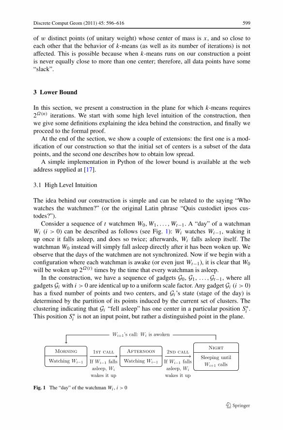
The idea behind our construction is simple and can be related to the saying “Whowatches the watchmen?” (or the original Latin phrase “Quis custodiet ipsos cus-todes?”).

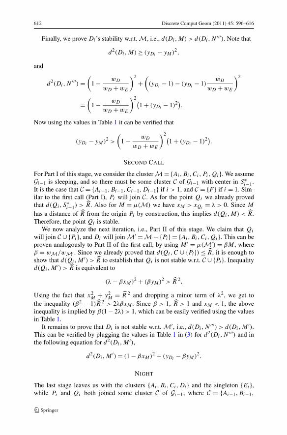
Consider a sequence of t watchmen W0,W1, . . . ,Wt−1. A “day” of a watchmanWi (i > 0) can be described as follows (see Fig. 1): Wi watches Wi−1, waking itup once it falls asleep, and does so twice; afterwards, Wi falls asleep itself. Thewatchman W0 instead will simply fall asleep directly after it has been woken up. Weobserve that the days of the watchmen are not synchronized. Now if we begin with aconfiguration where each watchman is awake (or even just Wt−1), it is clear that W0will be woken up 2Ω(t) times by the time that every watchman is asleep.

In the construction, we have a sequence of gadgets G0, G1, . . . , Gt−1, where allgadgets Gi with i > 0 are identical up to a uniform scale factor. Any gadget Gi (i > 0)has a fixed number of points and two centers, and Gi ’s state (stage of the day) isdetermined by the partition of its points induced by the current set of clusters. Theclustering indicating that Gi “fell asleep” has one center in a particular position S∗

i .This position S∗

i is not an input point, but rather a distinguished point in the plane.

Fig. 1 The “day” of the watchman Wi , i > 0


In the situation when Gi+1 is awake and Gi falls asleep, some points of Gi+1 willbe assigned temporarily to the center of Gi located in S∗

i ; in the next step this centerwill move so that in one more step the initial clustering (or “morning clustering”) ofGi is restored: this models the fact that Gi+1 wakes up Gi .

Note that since each gadget has a constant number of centers, we can build aninstance with k clusters that has t = Θ(k) gadgets, for which k-means will require2Ω(k) iterations. Also since each gadget has a constant number of points, we can buildan instance of n points and k = Θ(n) clusters with t = Θ(n) gadgets. This will implya lower bound of 2Ω(n) on the running time of k-means.

3.2 Definitions and Further Intuition

For any i > 0, the gadget Gi is a tuple (Pi , Ti , ri ,Ri) where each Pi ⊂ R2 is a set of

seven weighted points {Pi,Qi,Ai,Bi,Ci,Di,Ei}, while Ti is the set of initial centersof the gadget Gi and contains exactly two centers. Finally, ri ∈ R

+ and Ri ∈ R+

denote respectively the “inner radius” and the “outer radius” of the gadget, and theirpurpose will be explained later. Since the weights of the points do not change betweenthe gadgets, we will denote the weight of Pi (for any i > 0) with wP , and similarlyfor the other points.

As for the “leaf” gadget G0, the set P0 is composed of only one point F (of con-stant weight wF ), and T0 contains only one center.

The set of points of the k-means instance will be the union of the (weighted)points from all the gadgets, i.e.,

⋃t−1i=0 Pi (with a total of 7(t − 1) + 1 = O(t) points

of constant weight). Similarly, the set of initial centers will be the union of the centersfrom all the gadgets, that is,

⋃t−1i=0 Ti (with a total of 2(t − 1) + 1 = O(t) centers).

As we mentioned above, when one of the centers of Gi moves to a special locationcalled S∗

i , it will mean that Gi has fallen asleep. For i > 0 we define S∗i as the center

of mass of the subset {Ai,Bi,Ci,Di} of Pi , while S∗0 coincides with F . We stress

that, for i > 0, S∗i is not a point of the gadget Gi , but rather a special location in the

plane.For a gadget Gi (i > 0), we depict the stages (clusterings) it goes through during

any of its day. The entire sequence is shown in Fig. 2.

MORNING

This stage takes place right after Gi has been woken up or in the beginning ofthe entire process. The singleton {Ai} is one cluster, and the remaining points{Bi,Ci,Di,Ei,Pi,Qi} form the other cluster. In this configuration, Gi is watchingGi−1 and intervenes once it falls asleep.

FIRST CALL

Once Gi−1 falls asleep, Pi will join the cluster of Gi−1 cluster with center at S∗i−1

(Part I). At the next step (Part II), Qi too will join that cluster, and Bi will insteadmove to the cluster {Ai}. The two points Pi and Qi are waking up Gi−1 by causing arestoration of its morning clustering, as we will explain later.


Fig. 2 The “day” of the gadget Gi . The diamonds denote the centers of the clusters. The locations of thepoints in figure give an idea of the actual gadget used in the proof. Also, the bigger the size of a point, thegreater its weight

AFTERNOON

The points Pi , Qi and Ci will join the cluster {Ai,Bi}. Thus, Gi ends up with theclusters {Ai,Bi,Ci,Pi,Qi} and {Di,Ei}. In this configuration, Gi is again watchingGi−1 and is ready to wake it up once it falls asleep.

SECOND CALL

Once Gi−1 falls asleep, similarly to the first call, Pi will join the cluster of Gi−1 withcenter at S∗

i−1 (Part I). At the next step (Part II), Qi too will join that cluster, andDi will join the cluster {Ai,Bi,Ci} (note that the other cluster of Gi is the singleton{Ei}). Again, Pi and Qi are waking up Gi−1.

NIGHT

At this point, the cluster {Ai,Bi,Ci,Di} is already formed, which implies that itsmean is located in S∗

i : thus, Gi is sleeping. However, note that Pi and Qi are still insome cluster of Gi−1 and the remaining point Ei is in a singleton cluster. In the nextstep, concurrently with the beginning of a possible call from Gi+1 (see Gi+1’s call,Part I), the points Pi and Qi will join the singleton {Ei}.

The two radii of each gadget Gi (i > 0) can be interpreted in the following way.Whenever Gi is watching Gi−1 (either morning or afternoon), the distance betweenthe point Pi and its center will be exactly Ri . On the other hand, the distance betweenPi and S∗

i−1 – where one of the centers of Gi−1 will move when Gi−1 falls asleep—will be just a bit less than Ri . In this way, we guarantee that the waking-up process


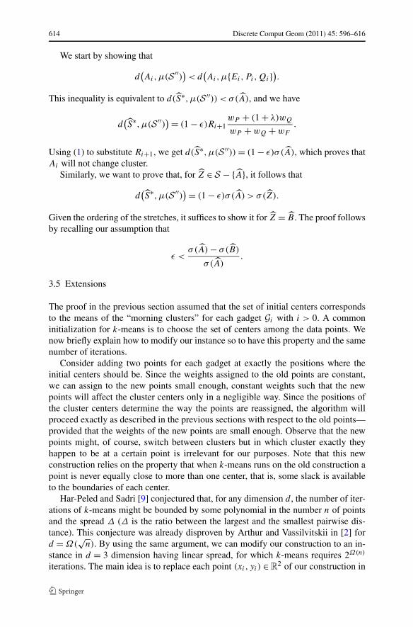
Fig. 3 Gi+1’S CALL: how Gi+1 wakes up Gi . The distance between the two gadgets is actually muchlarger than it appears in the figure

will start at the right time. Also, we know that this process will involve Qi too, andwe want the center that was originally in S∗

i−1 to end up at distance more than ri

from Pi . In that step, a center of Gi will be at distance exactly ri from Pi , and thus Pi

(and Qi too) will come back to one of the clusters of Gi .Now we analyze the waking-up process from the point of view of the sleeping

gadget. We suppose that Gi (i > 0) is sleeping and that Gi+1 wants to wake it up. Thesequence is shown in Fig. 3.

Gi+1’S CALL

Suppose that Gi+1 started to wake up Gi . Then, we know that Pi+1 joined the cluster{Ai,Bi,Ci,Di} (Part I). However, this does not cause any point from this cluster tomove to other clusters. On the other hand, as we said before, the points Pi and Qi will“come back” to Gi by joining the cluster {Ei}. At the next step (Part II), Qi+1 too willjoin the cluster {Ai,Bi,Ci,Di,Pi+1}. The new center will be in a position such that,in one more step (Part III), Bi,Ci and Di will move to the cluster {Pi,Qi,Ei}. Alsowe know that at that very same step, Pi+1 and Qi+1 will come back to some clusterof Gi+1: this implies that Gi will end up with the clusters {Bi,Ci,Di,Ei,Pi,Qi} and{Ai}, which is exactly the morning clustering: Gi has been woken up.

As for the “leaf” gadget G0, we said that it will fall asleep right after it has beenwoken up by G1. Thus we can describe its day in the following way.


G0’S NIGHT

There is only one cluster which is the singleton {F }. The center is obviously F whichcoincides with S∗

0 . In this configuration, G0 is sleeping.

G1’S CALL

The point P1 from G1 joins the cluster {P0} and in the next step Q1 will join the samecluster, too. After one more step, both P1 and Q1 will come back to some clusterof G1, which implies that the cluster of G0 is the singleton {F } again. Thus G0, afterhaving been temporarily woken up, falls asleep again.

3.3 Formal Construction

We start giving the distances between the points in a single gadget (intra-gadget). Af-terwards, we will give the distances between two consecutive gadgets (inter-gadget).Henceforth xAi

and yAiwill denote respectively the x-coordinate and y-coordinate

of the point Ai , and analogous notation will be used for the other points. Also, for aset of points S , we define its total weight

wS =∑

x∈Swx,

and its mean

μ(S) = 1

wS

∑

x∈Swx · x.

Observe that the total weight wS is a scalar, while the mean μ(S) is a point in theplane. As we will see in Sect. 3.4, the values assigned to wP ,wQ,wA, . . . in ourconstruction will be positive integers with the property that wA = wB and wF =wA + wB + wC + wD .

We start describing the distances between points for a non-leaf gadget. For sim-plicity, we start defining the location of the points for an hypothetical “unit” gadget Gthat has unitary inner radius (i.e., r = 1) and is centered in the origin (i.e., P = (0,0)).Then we will see how to define a gadget Gi (for any i > 0) in terms of the unit gad-get G .

The outer radius is defined as R = (1 + δ) and also we let the point Q be Q =(λ,0). The values 0 < δ < 1 and 0 < λ < 1 are constants whose exact values will beassigned later. The point E is defined as E = (0,1).

The remaining points are aligned on the vertical line with x-coordinates equal to 1.Formally,

xA = xB = xC = xD = 1.

As for the y-coordinates, we set yA = −1/2 and yB = 1/2.The value yC is uniquely defined by imposing yC > 0 and that the mean of the

cluster M = {A, B, C, P , Q} is at distance R from P . Thus, we want positive yC

that satisfies the equation ‖μ(M)‖ = R, which can be rewritten as


(wA + wB + wC + wQλ

wM

)2

+(

wCyC

wM

)2

= (1 + δ)2,

where we used the fact that wAyA + wByB = 0 when wA = wB . The first and thesecond term on the L.H.S. of the above equality correspond respectively to the x-coordinate and to the y-coordinate of μ(M).

We easily obtain the solution

yC = 1

wC

√(wM(1 + δ)

)2 − (wA + wB + wC + wQλ)2.

Note that the value under the square root is always positive because λ < 1.It remains to set yD . Its value is uniquely defined by imposing yD > 0 and that

the mean of the cluster N = {B, C, D, E, P , Q} is at distance R from P . Analo-gously to the previous case, yD is the positive value satisfying ‖μ(N )‖ = R, whichis equivalent to

(1 + δ)2 =(

wB + wC + wD + wQλ

wN

)2

+(

wDyD + wB(1/2) + wCyC + wE

wN

)2

.

Now, since the equation a2 + (b + x)2 = c2 has the solutions x = ±√c2 − a2 − b,

we obtain the solution

yD = 1

wD

√(wN (1 + δ)

)2 − (wB + wC + wD + wQλ)2 − wB/2 − wCyC − wE.

Again, the term under the square root is always positive.Finally, we define S∗ = μ{A, B, C, D}.Now consider a gadget Gi with i > 0. Suppose we have fixed the inner radius ri

and the center Pi . Then we have the outer radius Ri = (1 + δ)ri , and we define thelocation of the points in terms of the unit gadget by scaling of ri and translating byPi in following way: Ai = Pi + riA, Bi = Pi + riB , and so on for the other points.

As for the gadget G0, there are no intra-gadget distances to be defined, since it hasonly one point F .

For any i > 0, the intra-gadget distances in Gi have been defined (as a functionof Pi , ri , δ and λ). Now we define the (inter-gadget) distances between the points oftwo consecutive gadgets Gi and Gi+1, for any i ≥ 0. We do this by giving explicitrecursive expressions for ri and Pi .

For a point Z ∈ {A, B, C, D}, we define the “stretch” of Z (from S∗ with respectto μ{E, P , Q}) as

σ(Z) =√

d2(Z,μ{E, P , Q}) − d2(Z, S∗),

where d(·, ·) denotes the Euclidean distance between two points. The stretch willbe a real number (for all points A, B, C, D), given the values λ, δ and the weightsused in the construction. The values of the stretches will be used to characterize thereassignments of the points Ai , Bi , Ci , and Di when the gadget Gi+1 is waking upthe (sleeping) gadget Gi . Specifically, consider the cluster S = {Ai,Bi,Ci,Di} with


center in S∗i . As we will see later, for a point Z ∈ S , σ(Z) denotes how much the

center of S can be “pulled” by the (points of the) gadget Gi+1 before Z switches toanother cluster.

We set the inner radius r0 of the leaf gadget G0 to a positive arbitrary value, andfor any i ≥ 0, we define

ri+1 = ri

1 + δ

wF + wP + wQ

wP + (1 + λ)wQ

σ(A), (1)

where we recall that wF = wA +wB +wC +wD . Note that the ratio ri+1/ri betweenthe radii does not depend on i.

Recall that S∗i = μ{Ai,Bi,Ci,Di} for any i > 0, and S∗

0 = μ{F } = F . Assumingwe have fixed the point F somewhere in the plane, we define for any i > 0

xPi= xS∗

i−1+ Ri(1 − ε) = xS∗

i−1+ ri(1 + δ)(1 − ε) (2)

and

yPi= yS∗

i−1,

where 0 < ε < 1 is some constant to define. Note that now the instance is completelydefined as a function of λ, δ, ε and the weights. Their values are still undefined andwill be defined in Sect. 3.4. We are now ready to prove the lower bound.

3.4 Proof

We assume that the initial centers—that we seed k-means with—correspond to themeans of the “morning clusters” of each gadget Gi with i > 0. Namely, the initialcenters are μ{Ai}, μ{Bi,Ci,Di,Ei,Pi,Qi} for all i > 0, in addition to the centerμ{F } = F for the leaf gadget G0.

In order to establish our result, it is enough to show that there exist positive integervalues wA, wB , wC , wD , wE , wF , wP , wQ (with wA = wB ) and values for λ, δ andε, such that the behavior of k-means on the instance reflects exactly the clusteringtransitions described in Sect. 3.2.

3.4.1 Chosen Values

The chosen values (as well as other derived values used later in the analysis) are givenin Table 1. Also wF = wA + wB + wC + wD = 50. The use of rational weights isno restriction because the mean of a cluster (as well as k-means’ behavior) does notchange if we multiply the weights of its points by the same factor—in our case it isenough to multiply all the weights by 100 to obtain integer weights.

Recalling that ri/Ri+1 is a constant by (1), we impose the value ε to be

0 < ε < min

{1

2

(ri

Ri+1d(S∗, C)

)2

,σ (A) − σ(B)

σ (A),

λ

1 + δ,

1 − 1 + λ

1 + δ

(

1 + wP + wQ

wF

)}

.


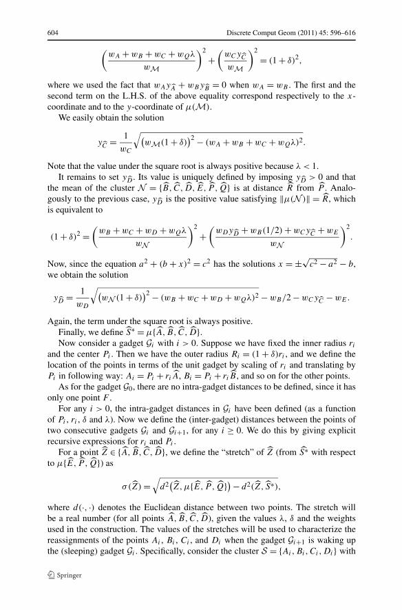
Table 1 The relation denotes the less-or-equal component-wise relation

Values Unit gadget

δ = 0.025 r = 1

λ = 10−5 R = (1 + δ) = 1.025

wP = 1 P = (0,0)

wQ = 10−2 Q = (λ,0) = (10−5,0)

wA = 4 A = (1,−0.5)

wB = 4 B = (1,0.5)

wC = 11 (1,0.70223) C (1,0.70224)

wD = 31 (1,1.35739) D (1,1.3574)

wE = 274 E = (0,1)

wF = 50 (1,0.996) S∗ (1,0.9961)

Clusters used in the proof

N = {Bi,Ci ,Di ,Ei ,Pi ,Qi } N ′ = {Bi,Ci ,Di ,Ei ,Qi }N ′′ = {Ci,Di,Ei } N ′′′ = {Di,Ei }M = {Ai,Bi ,Ci ,Pi ,Qi } M′ = {Ai,Bi ,Ci ,Qi }C =

{{Ai−1,Bi−1,Ci−1,Di−1}, i > 1

{F }, i = 1C′ = C ∪ {Pi,Qi }

S = {Ai,Bi ,Ci ,Di } S ′ = {Ai,Bi ,Ci ,Di ,Pi+1}S ′′ = {Ai,Bi ,Ci ,Di ,Pi+1,Qi+1}Derived values used in the proof

(0.1432,1.0149) N = μ(N ) (0.144,1.015)

(0.9495,0.386) M = μ(M) (0.9496,0.3861)

1.00312 ≤ α ≤ 1.00313

1.0526 ≤ β ≤ 1.05261

1.0003 ≤ σ(A) ≤ 1.0004

1.0001 ≤ σ(B) ≤ 1.0002

1 ≤ σ(C) ≤ 1.0001

0.9999 ≤ σ(D) ≤ 0.99992

0.99 ≤ γ ≤ 0.99047

All the terms on the right hand side of the above are clearly positive except for thelast one. In order to show that even the last term is indeed positive, we observe that(1 + δ)/(1 + λ) = 1 + (δ − λ)/(1 + λ). Therefore, the term can be rewritten as

1 −(

1 + wP + wQ

wF

)(

1 + δ − λ

1 + λ

)−1

,

which is positive when (δ − λ)/(1 + λ) > (wP + wQ)/wF . This last inequality canbe verified by plugging in the values from Table 1.


3.4.2 Stage-by-Stage Proof

Throughout the proof, we will say that a point Z in a cluster C is stable with respectto (w.r.t.) another cluster C′, if d(Z,μ(C)) < d(Z,μ(C′)). Similarly, a point Z in acluster C is stable if Z is stable w.r.t. any C′ �= C . Similar definitions of stability extendto a cluster or clustering if the stability holds for all the points in the cluster or all theclusters in the clustering.

Consider any stage of a gadget Gi (i > 1) and any stage of Gi+1. We observe thata point of Gi is always stable w.r.t. any cluster of Gi+1 since the distance from thispoint to its center is always at most 2ri , while its distance to any Gi+1’s center is atleast

d(Pi+1, S∗i ) = ri+1(1 − ε)

= ri1 − ε

1 + δ

wF + wP + wQ

wP + (1 + λ)wQ

σ(A)

> ri1

1 + δ

(

1 − σ(A) − σ(B)

σ (A)

)wF + wP + wQ

wP + (1 + λ)wQ

σ(A)

= ri1

1 + δ

wF + wP + wQ

wP + (1 + λ)wQ

σ(B) > 49ri,

where we used (1)–(2) and the assumption on ε (also refer to Figs. 2 and 3.) There-fore, in proving stability of a point (or cluster) of Gi , it will be enough to prove itsstability w.r.t. to clusters of Gi and Gi−1.

Note that the previous argument implies that a point of a gadget Gi is never as-signed to a cluster of Gi+1. On the contrary, we recall that points of Gi are indeedassigned to clusters of Gi−1 (during the waking-up process). Finally, we observe thatpoints of Gi are never assigned to a cluster of Gj with i − j ≥ 2 because by construc-tion these points are always closer to some center of Gi or Gi−1 than to any centerof Gj . Specifically, consider any point Z ∈ R

2 with xZ ≤ xS∗i−1

. In any stage of thegadget Gi , the points Ai,Bi,Ci,Di are at distance at most 1.5ri from their (Gi ’s)centers, while their distance from Z (and hence to any point of any Gj , j < i) is atleast 2ri . As for the point Ei , its distance from its (Gi ’s) center is always less than0.5ri (thanks to its large weight), while its distance from Z is at least ri . Observethat this means that all the points Ai,Bi,Ci,Di,Ei are never assigned to centers notbelonging to Gi . Finally, for Pi (resp., Qi ), there is always a center of Gi or Gi−1 atdistance at most (1 − ε)Ri (resp., at most (1 − ε)Ri + λri ) from it, while its distanceto any center of Gj with i − j ≥ 2 is at least (1 − ε)Ri + 2(1 − ε)Ri−1 (resp., at least(1 − ε)Ri + λri + 2(1 − ε)Ri−1). Therefore, we can conclude that gadgets Gi and Gj

with |i − j | ≥ 2 cannot interfere.For the proof, we will consider an arbitrary gadget Gi with i > 0 in any stage of its

day (some clustering), and we will show that the steps that k-means goes through areexactly the ones described in Sect. 3.2 for that stage of the day (for the chosen valuesof λ, δ, ε and weights). For the sake of convenience and w.l.o.g, we assume that Gi

has unitary inner radius (i.e., ri = r = 1 and Ri = R = (1 + δ)) and that Pi is in theorigin (i.e., Pi = (0,0)).


MORNING

We need to prove that the morning clustering of Gi is stable assuming that Gi−1 isnot sleeping. Note that this assumption implies that i > 1 since the gadget G0 isalways sleeping when G1 is in the morning. The singleton cluster {Ai} is triviallystable. Therefore, we just need to show that N = {Bi,Ci,Di,Ei,Pi,Qi} is stablew.r.t. to {Ai} and any cluster of Gi−1. In order to prove the stability of N w.r.t. {Ai},it suffices to show that Bi , Qi and Pi are stable w.r.t. {Ai} since the other pointsin N are further away from Ai . As for the stability of N w.r.t. a cluster of Gi−1,observe that it is enough to show that Pi is stable w.r.t. that cluster because the pointsBi,Ci,Di,Qi are further away from any center of Gi−1, while Ei is very close toits center (refer to Fig. 2, Morning, and values in Table 1). Letting N = μ(N ) andrecalling wN = 321.01, we have

xN = wB + wC + wD + λwQ

wN= 46.0000001

321.01≈ 0.1433,

and

yN =√

(1 + δ)2 − x2N ≈ 1.0149.

We have that N has a distance of R = (1 + δ) from the origin Pi by construction.Thus, the point Pi is stable w.r.t. {Ai} since

d(Pi,N) = R = (1 + δ) <√

12 + (0.5)2 = d(Pi,Ai).

To prove the same for Qi , note that

d(Qi,Ai) =√

(1 − λ)2 + (0.5)2 > R,

while, on the other hand, xN > xQiimplies d(Qi,N) < d(Pi,N) = R.

As for Bi , we have

d2(Bi,N) = (xB − xN)2 + (yB − yN)2

= ‖Bi‖2 + R 2 − 2(xNxBi+ yNyBi

).

With ‖B‖2 = 5/4, the inequality d(Bi,N) < d(Bi,Ai) = 1 simplifies to 5/4 + R 2 −2xN − yN < 1, which can be checked to be valid.

It remains to prove that Pi is stable w.r.t. any of Gi−1’s clusters. We observe that,in any stage of Gi−1’s day different from the night, one of Gi−1’s centers has x-coordinate and y-coordinate at most xCi−1 and less than yCi−1 , respectively, whilethe other center has x-coordinate at most yPi−1 + ri−1(wB + wC + wD)/wE <

yPi−1 +0.17ri−1 = yCi−1 −0.83ri−1 (refer to Fig. 2 and Table 1.) Taking into accountthat d(S∗

i−1,Ci−1) < 0.3ri−1 < 0.83ri−1 and that yS∗i−1

= yPi, the above observation

implies that the distance from Pi to any center of Gi−1 is more than the distance fromPi to Ci−1. Using (2) and recalling that xCi−1 = xS∗

i−1, Pythagorean theorem yields


d2(Pi,Ci−1) = (xPi− xS∗

i−1)2 + d2(S∗

i−1,Ci−1)

= R2i (1 − ε)2 + r2

i−1d2(S∗, C).

Thus, a sufficient condition for the inequality d2(Pi,Ci−1) > R2i = d2(Pi,N) is

2εR2i < r2

i−1d2(S∗, C),

or

ε <1

2

(ri−1

Ri

d(S∗, C)

)2

,

which is true by the assumption on ε.

FIRST CALL

We start by analyzing Part I of this stage. Since we are assuming that Gi−1 is sleeping,there must be some cluster C of Gi−1 with center in S∗

i−1. Specifically,

C ={{

{Ai−1,Bi−1,Ci−1,Di−1}, if i > 1,

{F }, if i = 1.

Note that, in both cases, wC = 50. By (2), we have d(Pi, S∗i−1) < Ri , and so Pi will

join C . We claim that Qi is instead stable, i.e., d(Qi,N) < d(Qi, S∗i−1); this implies

that all other points of Gi are stable as well. We already know that d(Qi,N) < R, sowe show d(Qi, S

∗i−1) > R. Using (2), we have

d(Qi, S∗i−1) = R(1 − ε) + λr > R,

which holds since ε < λ/(1 + δ).We now analyze the next iteration, i.e., Part II of this stage. We claim that Qi

will join C ∪ {Pi}, and Bi will join {Ai}. To establish the former, we show that (a)d(Qi,μ(C ∪ {Pi})) < R and that (b) d(Qi,μ(N ′)) > R where N ′ = N − {Pi} ={Bi,Ci,Di,Ei,Qi}. For (a) observe that

d(Qi,μ

(C ∪ {Pi}

)) = λ + d(Pi,μ

(C ∪ {Pi}

)) = λ + d(Pi,μ(C)

)(1 − wP /wC )

= λ + Ri(1 − ε)(1 − wP /wC ) < Ri + λ − RiwP /wC

< R + λ − wP /wC < R,

where we used (2), and the last step follows by plugging in the values λ = 10−5,wP = 1 and wC = 50. As for (b), since Pi is in the origin we can write N ′ = αN withα = wN /wN ′ . Thus, the inequality we are interested in is

(λ − αxN)2 + (αyN)2︸︷︷︸

d2(Qi,μ(N ′))

> R 2.


Using the fact that x2N + y2

N = R 2 and dropping a minor term of λ2, we get to theinequality (α2 − 1)R 2 > 2λαxN . Observe that α > 1 implies α2 > α. Using thisand recalling that R > 1 and xN < 1, we conclude that the inequality is implied byα(1 − 2λ) > 1, which holds for the chosen values.

It remains to prove that Bi is not stable w.r.t. {Ai}, i.e., d(Bi,N′) > d(Bi,Ai) = 1.

We need to prove the validity of the inequality

(1 − αxN)2 + (1/2 − αyN)2 > 1.

This can be easily verified by plugging in the upper bounds for the values α, xN

and yN .Finally, we prove that Ci is instead stable w.r.t. N ′, i.e.,

(xCi− αxN)2 + (yCi

− αyN)2 < (yCi− yAi

)2.

Since Pi is in the origin, we can plug in the values xCi= 1 and yAi

= 1/2. Also,recalling that x2

N + y2N = R 2, we obtain

3

4+ α2R 2 − 2αxN < yCi

(1 + 2αyN),

which is implied by

3

4+ α2R 2 < yCi

(1 + 2αyN).

Again, the values in Table 1 satisfy this last inequality.

AFTERNOON

The last stage ended up with the Gi ’s clusters {Ai,Bi} and N ′′ = {Ci,Di,Ei}, sincePi and Qi both joined some cluster C of Gi−1. Specifically,

C ={

{Ai−1,Bi−1,Ci−1,Di−1}, if i > 1,

{F }, if i = 1.

We claim that, at this point, Pi,Qi and Ci are not stable and will all join the cluster{Ai,Bi}.

Let C′ = C ∪ {Pi,Qi}; note that the total weight wC′ of the cluster C′ is the sameif Gi−1 is the leaf gadget G0 or not, since by definition

wC = wF = wA + wB + wC + wD = 50.

We start showing that d(Pi,μ(C′)) > r = 1 which proves that the claim is true for Pi

and Qi . By defining d = xPi− xS∗

i−1, the inequality can be rewritten as

d − wP d + wQ(d + λ)

wC′> 1.


By (2) and the definition of Ri = R, we have d = (1 + δ)(1 − ε). Therefore, sincewC = wC′ − wP − wQ, the above inequality is equivalent to

(1 − ε)(1 + δ)wCwC′

> 1 + λwQ

wC′,

which is implied by

(1 − ε)(1 + δ)wCwC′

> 1 + λ,

since wQ = 10−2 and wC′ = wC +wP +wQ = 50+1+0.01 = 51.01. Now considerthe inequality

(1 + δ)wCwC′

> 1 + λ.

By plugging in the values δ = 0.025, λ = 10−5 and wC /wC′ = 50/51.01 > 0.98, theabove inequality is satisfied. Therefore, it suffices to have

ε < 1 − 1 + λ

1 + δ

wC′

wC,

which is provided by the assumption on ε.Now we prove that Ci is not stable w.r.t. to {Ai,Bi}, by showing that d(Ci,N

′′) >

yCiwhere N ′′ = μ(N ′′). Note that the inequality is implied by xCi

− xN ′′ > yCi,

which is equivalent towE

wN ′′> yCi

,

which holds for the chosen values.At this point, analogously to the morning stage, we want to show that this new

clustering is stable, assuming that Gi−1 is not sleeping. Note that the analysis inthe morning stage directly implies that Pi is stable w.r.t. any of Gi−1’s clusters. Itremains to prove that Pi is stable w.r.t. to N ′′′ = {Di,Ei}, and Di is stable w.r.t.M = {Ai,Bi,Ci,Pi,Qi} (other points’ stability is implied).

As for the former, let M = μ(M) and N ′′′ = μ(N ′′′). Since d(Pi,N′′′) = ‖N ′′′‖,

we have

d2(Pi,N′′′) =

(wD

wE + wD

)2

+(

wE + yDiwD

wE + wD

)2

= 1

(wE + wD)2

(w2

D + w2E + y2

Diw2

D + 2wEwD + 2(yDi− 1)wEwD

)

= 1 + y2Di

w2D + 2(yDi

− 1)wEwD

(wE + wD)2≥ 1 + 2(yDi

− 1)wEwD

(wE + wD)2. (3)

Since d(Pi,M) = 1+ δ, in order to prove d(Pi,N′′′) > d(Pi,M), it suffices to verify

that

2(yDi− 1)wEwD

(wE + wD)2> 2δ + δ2,

which can be checked using the values in Table 1.


Finally, we prove Di ’s stability w.r.t. M, i.e., d(Di,M) > d(Di,N′′′). Note that

d2(Di,M) ≥ (yDi− yM)2,

and

d2(Di,N′′′) =

(

1 − wD

wD + wE

)2

+(

(yDi− 1) − (yDi

− 1)wD

wD + wE

)2

=(

1 − wD

wD + wE

)2(1 + (yDi

− 1)2).

Now using the values in Table 1 it can be verified that

(yDi− yM)2 >

(

1 − wD

wD + wE

)2(1 + (yDi

− 1)2).

SECOND CALL

For Part I of this stage, we consider the cluster M = {Ai,Bi,Ci,Pi,Qi}. We assumeGi−1 is sleeping, and so there must be some cluster C of Gi−1 with center in S∗

i−1.It is the case that C = {Ai−1,Bi−1,Ci−1,Di−1} if i > 1, and C = {F } if i = 1. Sim-ilar to the first call (Part I), Pi will join C . As for the point Qi we already provedthat d(Qi, S

∗i−1) > R. Also for M = μ(M) we have xM > xQi

= λ > 0. Since M

has a distance of R from the origin Pi by construction, this implies d(Qi,M) < R.Therefore, the point Qi is stable.

We now analyze the next iteration, i.e., Part II of this stage. We claim that Qi

will join C ∪ {Pi}, and Di will join M′ = M − {Pi} = {Ai,Bi,Ci,Qi}. This can beproven analogously to Part II of the first call, by using M ′ = μ(M′) = βM , whereβ = wM/wM′ . Since we already proved that d(Qi,C ∪ {Pi}) ≤ R, it is enough toshow that d(Qi,M

′) > R to establish that Qi is not stable w.r.t. C ∪ {Pi}. Inequalityd(Qi,M

′) > R is equivalent to

(λ − βxM)2 + (βyM)2 > R 2.

Using the fact that x2M + y2

M = R 2 and dropping a minor term of λ2, we get tothe inequality (β2 − 1)R 2 > 2λβxM . Since β > 1, R > 1 and xM < 1, the aboveinequality is implied by β(1 − 2λ) > 1, which can be easily verified using the valuesin Table 1.

It remains to prove that Di is not stable w.r.t. M′, i.e., d(Di,N′′′) > d(Di,M

′).This can be verified by plugging the values in Table 1 in (3) for d2(Di,N

′′′) and inthe following equation for d2(Di,M

′),

d2(Di,M′) = (1 − βxM)2 + (yDi

− βyM)2.

NIGHT

The last stage leaves us with the clusters {Ai,Bi,Ci,Di} and the singleton {Ei},while Pi and Qi both joined some cluster C of Gi−1, where C = {Ai−1,Bi−1,


Ci−1,Di−1} if i > 1 and C = {F } if i = 1. We want to prove that in one iteration Pi

and Qi will join {Ei}. Consider the cluster C′ = C ∪ {Pi,Qi}. In the afternoon stage,we already proved that d(Pi,μ(C′)) > r , and since d(Pi,Ei) = r = 1, the point Pi

will join {Ei}. For the point Qi , we have

d(Qi,μ(C′)

) = d(Pi,μ(C′)

) + λ > r + λ,

while

d(Qi,Ei) =√

r2 + λ2 < r + λ.

Thus, the point Qi , as well as Pi , will join {Ei}.Gi+1’S CALL

In this stage, we are analyzing the waking-up process from the point of view of thesleeping gadget. We fix any i > 0 and suppose that Gi is sleeping and that Gi+1wants to wake it up. Again w.l.o.g. we assume that Gi has unitary inner radius (i.e.,ri = r = 1 and Ri = R = (1 + δ)) and that Pi is in the origin (i.e., Pi = (0,0)).

We start by considering Part I of this stage, when Pi+1 (only) joined the clus-ter S = {Ai,Bi,Ci,Di}, while Pi and Qi joined the cluster {Ei}. Let S ′ = S ∪{Pi+1} = {Ai,Bi,Ci,Di,Pi+1}. We want to verify that the points in S are stablew.r.t. {Ei,Pi,Qi}, i.e., that for each Z ∈ S ,

d(Z,μ(S ′)

)< d

(Z,μ{Ei,Pi,Qi}

).

Recall that S∗i = μ{Ai,Bi,Ci,Di} = μ(S). By Pythagorean theorem and yPi+1 =

yS∗i,

d2(Z,μ(S ′)) = d2(Z, S∗) + d2(S∗,μ(S ′)

).

Therefore, by rearranging the terms and the definition of σ(Z), the above inequalityis equivalent to d(S∗,μ(S ′)) < σ(Z). Given the ordering of the stretches, it is enoughto show it for Z = D. By (2) and yPi+1 = yS∗

i, we have that

d(S∗,μ(S ′)

) = (1 − ε)Ri+1wP

wS ′.

Also, using (1), we get

d(S∗,μ(S ′)

) = r(1 − ε)γ σ (A),

where

γ = wP

wS ′· wS ′ + wQ

wP + (1 + λ)wQ

.

Finally, it is easy to verify that γ σ(A) < σ(D).In Part II of this stage, Qi+1 joined S ′. Let S ′′ = S ′ ∪ {Qi+1} = {Ai,Bi,Ci,Di,

Pi+1,Qi+1}. We want to verify that all the points in S but Ai will move to the cluster{Ei,Pi,Qi}.


We start by showing that

d(Ai,μ(S ′′)

)< d

(Ai,μ{Ei,Pi,Qi}

).

This inequality is equivalent to d(S∗,μ(S ′′)) < σ(A), and we have

d(S∗,μ(S ′′)

) = (1 − ε)Ri+1wP + (1 + λ)wQ

wP + wQ + wF

.

Using (1) to substitute Ri+1, we get d(S∗,μ(S ′′)) = (1 − ε)σ (A), which proves thatAi will not change cluster.

Similarly, we want to prove that, for Z ∈ S − {A}, it follows that

d(S∗,μ(S ′′)

) = (1 − ε)σ (A) > σ(Z).

Given the ordering of the stretches, it suffices to show it for Z = B . The proof followsby recalling our assumption that

ε <σ(A) − σ(B)

σ (A).

3.5 Extensions

The proof in the previous section assumed that the set of initial centers correspondsto the means of the “morning clusters” for each gadget Gi with i > 0. A commoninitialization for k-means is to choose the set of centers among the data points. Wenow briefly explain how to modify our instance so to have this property and the samenumber of iterations.

Consider adding two points for each gadget at exactly the positions where theinitial centers should be. Since the weights assigned to the old points are constant,we can assign to the new points small enough, constant weights such that the newpoints will affect the cluster centers only in a negligible way. Since the positions ofthe cluster centers determine the way the points are reassigned, the algorithm willproceed exactly as described in the previous sections with respect to the old points—provided that the weights of the new points are small enough. Observe that the newpoints might, of course, switch between clusters but in which cluster exactly theyhappen to be at a certain point is irrelevant for our purposes. Note that this newconstruction relies on the property that when k-means runs on the old construction apoint is never equally close to more than one center, that is, some slack is availableto the boundaries of each center.

Har-Peled and Sadri [9] conjectured that, for any dimension d , the number of iter-ations of k-means might be bounded by some polynomial in the number n of pointsand the spread Δ (Δ is the ratio between the largest and the smallest pairwise dis-tance). This conjecture was already disproven by Arthur and Vassilvitskii in [2] ford = Ω(

√n). By using the same argument, we can modify our construction to an in-

stance in d = 3 dimension having linear spread, for which k-means requires 2Ω(n)

iterations. The main idea is to replace each point (xi, yi) ∈ R2 of our construction in


d = 2 dimensions with two points (xi, yi, zi) and (xi, yi,−zi) in d = 3 dimensions,where zi = i · Δ and Δ is the spread in our original construction: note that, assumingthe smallest pairwise distance in the original instance is 1, we would have for thenew instance a smallest and largest pairwise distance of Ω(Δ) and O(nΔ), respec-tively. We observe that, even if this spread-reduction technique does not account forweighted points (because the spread of the given construction would be infinite), wecan simulate integer weights in the range [1,C] by blowing up the size of the dataset by at most C. Thus, the conjecture by Har-Peled and Sadri does not hold for anyd ≥ 3.

4 Conclusions

We presented how to construct a two-dimensional instance with k clusters for whichthe k-means algorithm requires 2Ω(k) iterations. For k = Θ(n), we obtain the lowerbound 2Ω(n). Our result improves the best known lower bound [2] in terms of numberof iterations (from 2Ω(

√n) to 2Ω(n)), as well as in terms of dimensionality (from

d = Ω(√

n) to d ≥ 2).We observe that in our construction each gadget uses a constant number of points

and wakes up the next gadget twice. For k = o(n), we could use Θ(n/k) points foreach gadget, and it would be interesting to see if one can construct a gadget with thismany points that is able to wake up the next one Ω(n/k) times. Note that this wouldgive the lower bound (n/k)Ω(n/k), which for k = nc (0 < c < 1), simplifies to nΩ(k).This matches the optimal upper bound O(nkd), as long as the construction lies in aconstant number of dimensions.

Acknowledgements I greatly thank Flavio Chierichetti and Sanjoy Dasgupta for their helpful commentsand discussions. I also thank David Arthur for having confirmed some intuitions on the proof in [2].

Open Access This article is distributed under the terms of the Creative Commons Attribution Noncom-mercial License which permits any noncommercial use, distribution, and reproduction in any medium,provided the original author(s) and source are credited.

References

1. Agarwal, P.K., Mustafa, N.H.: k-means projective clustering. In: Proceedings of the 23rd Symposiumon Principles of Database Systems, pp. 155–165 (2004)

2. Arthur, D., Vassilvitskii, S.: How slow is the k-means method. In: Proceedings of the 22nd AnnualSymposium on Computational Geometry, pp. 144–153 (2006)

3. Arthur, D., Vassilvitskii, S.: Worst-case and smoothed analysis of the ICP algorithm, with an applica-tion to the k-means method. SIAM J. Comput. 39(2), 766–782 (2009)

4. Arthur, D., Manthey, B., Röglin, H.: k-means has polynomial smoothed complexity. In: Proceedingsof the 50th Annual IEEE Symposium on Foundations of Computer Science (2009)

5. Berkhin, P.: Survey of clustering data mining techniques. Technical report, Accrue Software, San Jose,CA, USA (2002)

6. Duda, R.O., Hart, P.E., Stork, D.G.: Pattern Classification. Wiley, New York (2000)7. Forgy, E.W.: Cluster analysis of multivariate data: efficiency versus interpretability of classifications.

In: Biometric Society Meeting, Riverside, California, 1965. Abstract in Biometrics, vol. 21, p. 768(1965)


8. Gibou, F., Fedkiw, R.: A fast hybrid k-means level set algorithm for segmentation. In: Proceedings ofthe 4th Annual Hawaii International Conference on Statistics and Mathematics, pp. 281–291 (2005)

9. Har-Peled, S., Sadri, B.: How fast is the k-means method? Algorithmica 41(3), 185–202 (2005)10. Inaba, M., Katoh, N., Imai, H.: Variance-based k-clustering algorithms by Voronoi diagrams and

randomization. IEICE Trans. Inf. Syst. E83-D(6), 1199–1206 (2000)11. Kanungo, T., Mount, D.M., Netanyahu, N.S., Piatko, C.D., Silverman, R., Wu, A.Y.: A local search

approximation algorithm for k-means clustering. Comput. Geom. 28(2–3), 89–112 (2004)12. Lloyd, S.P.: Least squares quantization in PCM. IEEE Trans. Inf. Theory 28(2), 129–136 (1982)13. MacQueen, J.B.: Some methods for classification and analysis of multivariate observations. In: Pro-

ceedings of the 5th Berkeley Symposium on Mathematical Statistics and Probability, vol. 1, pp. 281–297 (1967)

14. Manthey, B., Röglin, H.: Improved smoothed analysis of the k-means method. In: Proceedings of the20th Annual Symposium on Discrete Algorithms, pp. 461–470 (2009)

15. Spielman, D.A., Teng, S.: Smoothed analysis of algorithms: why the simplex algorithm usually takespolynomial time. J. ACM 51(3), 385–463 (2004)

16. Vattani, A.: k-means requires exponentially many iterations even in the plane. In: Proceedings of the25th Annual Symposium on Computational Geometry, pp. 324–332. (2009)

17. Vattani, A.: k-means lower bound implementation, www.cse.ucsd.edu/~avattani/k-means/lowerbound.py

http://www.cse.ucsd.edu/~avattani/k-means/lowerbound.py

http://www.cse.ucsd.edu/~avattani/k-means/lowerbound.py

k-means Requires Exponentially Many Iterations...

Documents

Transcript of k-means Requires Exponentially Many Iterations...