K. M. Isaac Professor of Aerospace...

December 21, 2001 topic13_grid_generation 1

AE/ME 339

K. M. IsaacProfessor of Aerospace Engineering


Computational Fluid Dynamics (AE/ME 339) K. M. IsaacMAEEM Dept., UMR

The basic idea behind grid generation is the creation of the transformationlaws between the physical space and the computational space.

These laws are known as the metrics of the transformation.

We have already performed a simple grid generation without realizing itfor the flow over a heated wall when we used the �, �� coordinates for thenumerical scheme. This was simply a transformation from one rectangulardomain to another rectangular domain.



Grid Generation (Chapter 5)

Quality of the CFD solution is strongly dependent on the quality of thegrid.Why is grid generation necessary? Figure 5.1(next slide)can be used to explain.Note that the standard finite difference methods require a uniformlyspaced rectangular grid.If a rectangular grid is used, few grid points fall on the surface. Flow close to the surface being very important in terms of forces, heat transfer, etc., a rectangular grid will give poor results in suchregions.Also uniform grid spacing often does not yield accurate solutions.

Typically, the grid will be closely spaced in boundary layers.



Figure shows a physical flowdomain that surrounds the bodyand the corresponding rectangularflow domain.Note that if the airfoil is cut and the surface straightened out, itwould form the �-axis.Similarly, the outer boundarywould become the top boundaryof the computational domain.The left and right boundaries ofthe computational domain wouldrepresent the cut surface.Note the locations of points a, b,and c in the two figures.



Note that in the physical space the cells are not rectangular and the gridis uniformly spaced.There is a one-to-one correspondence between the physical space and thecomputational space. Each point in the computational space representsa point in the physical space.

The procedure is as follows:

1. Establish the necessary transformation relations between the physicalspace and the computational space

2. Transform the governing equations and the boundary conditions intothe computational space.

3. Solve the equations in the computational space using the uniformlyspaced rectangular grid.

4. Perform a reverse transformation to represent the flow propertiesin the physical space.



General Transformation RelationsConsider a two-dimensional unsteady flow with independent variablest, x, y.The variables in the computational domain are represented by �, �� andThe relations between the two sets of variables can be represented as

follows.� �...........................(5.1 )t c� ��

� �, , ...........................(5.1 )x y t a� ��

� �, , ...........................(5.1 )x y t b� ��



The derivatives appearing in the governing equations must be transformedusing the chain rule of differentiation.

, , , , ,, ,y t y t y t y tx x x x� ��

� � �

� � �

� � � ��

� � � � � � ��

The subscripts are used to emphasize significance of the partial derivativesand they will not be included in the equations that follow.



...........................(5.2)x x x

� �

� �

� � � ��

� � � � ��

...................(5.3)y y y

� �

� �

� � � ��

� � � � ��

, , , , ,, ,

.................(5.4)x y x y x y x yt t t t� ��

� � �

� � �

� � � ��

� � � � � � ��

.................(5.5)t t t t

� � �

� � �

� � � ��

� � � � � � ��



The first derivatives in the governing equations can be transformed usingEqs. (5.2), (5.3) and (5.5).

The coefficients of the transformed derivatives such as the ones givenbelow are known metrics.

, , ,x y x y� � � ��

� � � �

Similarly, chain rule should be used to transform higher order derivatives.Example:

22 2 2 2

2 2 2 2x x x x� � �

� � �

� � � � � ��

� � � � � � ��

22 2

2 .......................(5.9)x x x� � �

� � �

� � � ��

� � � � � ��



Metrics and Jacobian (5.3)In CFD the metric terms are not often available as analytical expressions.Instead they are often represented numerically.The following inverse transformation is often more convenient to use thanthe original transformation

� �, , ..........................(5.18 )x x a� � ��

� �, , .............................(5.18 )y y b� � ��

� �.............................(5.18 )t t c��



Let x = x(��), y = y(��) and u = u(x, y).then we can write

.................................(5.19)u udu dx dyx y

� ��

............................(5.21)u u x u yx y� � �

� � � � ��

� � � � �

............................(5.20)u u x u yx y� � �

� � � � ��

� � � � �

Eqs. (5.21) and (5.22) are two equations for the two unknown derivatives.



Solving for the partial derivatew. r. t x gives, using Cramer’srule

....................................(5.22)

u y

u yu

x yx

x y

� �

� �

� �

� �

� �

� �

� �

� ��

� ��

� �

� �

� �

� �

� �

,................................(5.22 )

,

x yx y

J ax y� �

� �

� �

� �

� ��

� ��

� �

Define the Jacobian J as

1 .............................(5.23 )u u y u y ax J � � � �

� ��

� � � � �� Eq. (5.22) can now bewritten in terms of J.



Similarly we can write the derivative w.r.t y as

1 .............................(5.23 )u u x u x by J � � � �

� ��

� � � � ��

and we can define the following

1 .............................(5.24 )u y y ax J � � � �

� ��

� � � � ��

1 .............................(5.24 )x x by J � � � �

� ��

� � � � ��



The above equations can be easily extended to three space dimensions(x, y an z).The above equations can also be obtained formally as follows

� �, ........................(5.25 )x y a� ��

.................................(5.26 )d dx dy ax y� �

��

� ��

� �, ........................(5.25 )x y b� ��

.................................(5.26 )d dx dy bx y� �

��

� ��

.......................................(5.27)d dxx yd dy

x y

� �

�

� � �

� ��



Similarly

� �, ...................................(5.28 )x x a� ��

� �, ...................................(5.28 )y y b� ��

.................................(5.29 )x xdx d d a� ��

� ��

.................................(5.29 )y ydy d d b� ��

� ��

.......................................(5.30)

x xdx ddy y x d

��

�

� �

� ��



Eq. (5.30) can be solved for d�, d�

1

.......................................(5.31)

x xd dxd y x dy� � �

�

� �

�

� ��

Consider the conservation form 2D flow with no source term

0...............................(5.37)U F Gt x y

� � ��

� � �



1

...............................(5.32)

x xx y

y yx y

� �

� �

� �

� �

�

� � � ��

Using results from matrix algebra for inversion of matrices, RHScan be written as follows

............................(5.33)

y x

y xx y

x xx y

y y

� �

� �

� �

� �

� �

� �

� ��

� ��

��

� � � ��

� �



Since the determinant of a matrix and its transpose are the same we can write

............................(5.34)

x x x y

Jy y x y� � � �

� � � �

� � � �

� � � ��

� � � �

� � � �

Substitute Eq. (5.34) into Eq. (5.33)

1 .................................(5.35)

y xx y

y xJx y

� �

� �

� �

� �

� � � ��

� � � ��

��



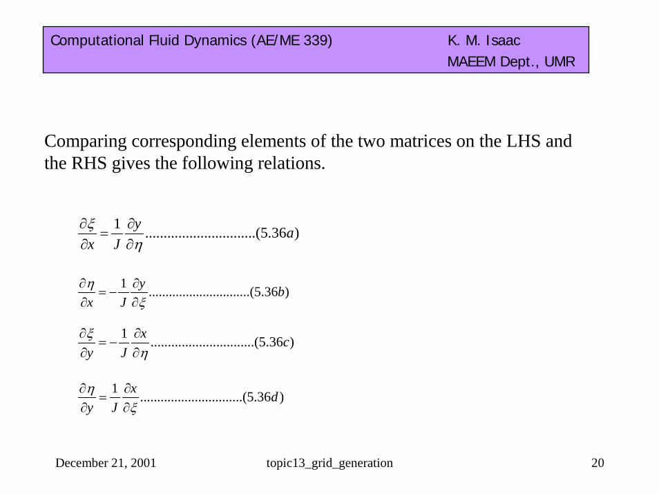
Comparing corresponding elements of the two matrices on the LHS andthe RHS gives the following relations.

1 .......................yx J�

�

� ��

� �.......(5.36 )a

1 ..............................(5.36 )y bx J�

�

� ��

� �

1 ..............................(5.36 )x cy J�

�

� ��

� �

1 ..............................(5.36 )x dy J�

�

� ��

� �



Consider the conservation form 2D flow with no source term

0...............................(5.37)U F Gt x y

� � ��

� � �



The above equation can be transformed to (see section 5.4)

1 1 1 0...............................(5.38)U F Gt � �

� � ��

� � �

Where the U1, F1, and G1 are as follows

1 ............................(5.48 )U JU a�

1 ................................(5.48 )F JF JG bx y� ��

� ��

1 ............................(5.48 )G JF JG cx y� ��

� ��



Algebraic Methods

Known functions are used to map irregular physical domain into rectangular computational domains.



Example: Grid stretchingmay be necessary for someproblems such as flow withboundary layers.Let us consider the trans-formation:

.....(5.50 )ln( 1).....(5.50 )x a

y b�

�

�

� �

Inverse transformation

.....(5.51 )exp( ) 1.....(5.51 )

x ay b

�

�

�

� �



The following relation (Eq. 5.52) hold between increments �y and ��

dy ed

�

��

dy e d��

..............................(5.52)y e� ��



Therefore as � increases, �y increases exponentially.Thus we can choose �� constant and still have an exponential stretchingof the grid in the y-direction.

)53.5.......(0)()(

)()(

��

��

�

�

yv

xu ��

)554......(0)()()()(�

�

�

�

��

�

�

�

��

�

�

�

��

�

�

�

�

yv

yv

xu

xu �

�

��

�

��

�

��

�

�

1��

�

x� 0�

�

�

y� 0�

�

�

x�

yy ��

�

�

11� ……(5.55)



Substitute in Eq. (5.54) to get

)56.5.......(0)(1

1)(�

�

�

��

�

�

�

�

�

� vy

u

)57.5.......(0)(1)(�

�

��

�

�

�

�

�

��

ve

u

0)()(�

�

��

�

�

�

�

�

�� vue

Eq. (5.57) is the continuity equation in the computational domain.Thus we have transformed the continuity equation from the physicalspace to the computational space.



The metrics carry the specifics of a particular transformation.

Boundary Fitted Coordinate System (5.7)

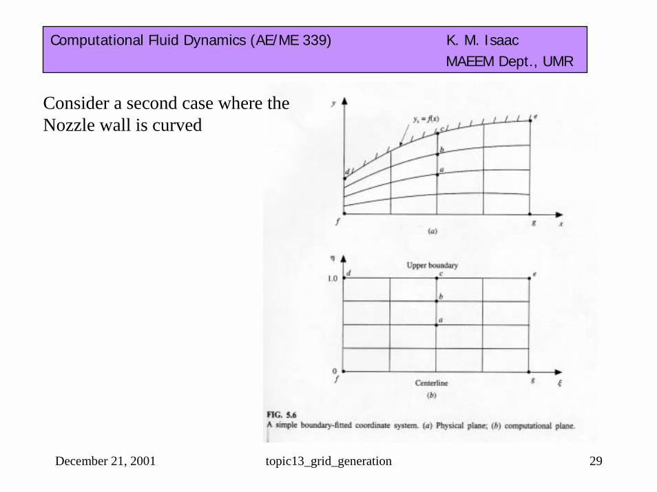
Here we consider the flow through a divergent duct as given in Figure 5.6 (next slide). de is the curved upper wall and fg is the centerline.Let ys = f(x) be the function that represents the upper wall.The following transformation will give rise to a rectangular grid.

� = x (5.65)� = y/ys (5.66)

To test this choose ys = 1.5x and let x vary from 1 to 5.At x = 1, � = 1, �max = ymax/ys = 1, and x = 5, � = 5, �max = ymax/ys = 1.

Thus the irregular domain is transformed into into a rectangular domain.



Consider a second case where the Nozzle wall is curved



2max

2max

3

2 2

.......1 2

1, 0

2 2 2

1 1

y x xx

y yy x

x yy

x x x

y x

�

�

� �

� � �

�

�

�

� � �

�

� �

� ��

� �

��

�

��

�



The above formulation is analytic

yxyx �� ,,,

The Jacobian is defined as

Could also be obtained using central differencing.

xyyx

yx

yxyx

J ��

��

��

�

�

�

�

�

�

�

�

��

��

),(),(



Let � = 1.75, � = 0.75Consider a point in the domain where we haveLet us calculate �_x analytically and numerically.

At this point:

2 2

1.750.75 (1.75) 2.29688

0.752 2 0.857151.75

1.0, 0

x

xy x

x y� �

�

��

�

�

� � � �

� � � � � � �

� �



We can also numerically calculate the derivatives using CD

1

max

max

3.0625 1.53125 3.06252 0.25

1 3.0625 0 0 3.0625

1.5 : 2.25 0.75 1.68752 : 4 0.75 3.0

3.0 1.6875 2.6252.0 1.5

2.625 0.857143.0625x

yy

I J x y y xy y

y yyy

yI

�

� � � �

�

�

�

� �

� �

�

�

�

� ��

� � � � � � � �

� � � � �

� � � � �

� ��

� � � � � �

K. M. Isaac Professor of Aerospace...

Documents

Transcript of K. M. Isaac Professor of Aerospace...