June 27-30, 2011, Taipei, Taiwan Fuzzy C-Means Clustering ...

2011 IEEE International Conference on Fuzzy SystemsJune 27-30, 2011, Taipei, Taiwan

978-1-4244-7316-8/11/$26.00 ©2011 IEEE

Fuzzy C-Means Clustering and Partition Entropyfor Species-Best Strategy and Search Mode Selectionin Nonlinear Optimization by Differential Evolution

Tetsuyuki TakahamaDepartment of Intelligent Systems

Hiroshima City UniversityAsaminami-ku, Hiroshima, 731-3194 JapanEmail: [email protected]

Setsuko SakaiFaculty of Commercial Sciences

Hiroshima Shudo UniversityAsaminami-ku, Hiroshima, 731-3195 Japan

Email: [email protected]

Abstract— Differential Evolution (DE) is a newly proposedevolutionary algorithm. DE is a stochastic direct search methodusing a population or multiple search points. DE has beensuccessfully applied to optimization problems including non-linear, non-differentiable, non-convex and multimodal functions.However, the performance of DE degrades in problems havingstrong dependence among variables, where variables are relatedstrongly to each other. In this study, we propose to utilize partitionentropy given by fuzzy clustering for solving the degradation.It is thought that a directional search is desirable when searchpoints are distributed with bias. Thus, when the entropy is low,algorithm parameters can be controlled to make the directionalsearch. Also, we propose to use a species-best strategy forimproving the efficiency and the robustness of DE. The effectof the proposed method is shown by solving some benchmarkproblems.

Index Terms—differential evolution; rotation-invariant; inten-sive search; extensive search

I. INTRODUCTION

Optimization problems, especially nonlinear optimizationproblems, are very important and frequently appear in thereal world. There exist many studies on solving optimizationproblems using evolutionary algorithms (EAs). Differentialevolution (DE) is a newly proposed EA by Storn and Price[1]. DE is a stochastic direct search method using a populationor multiple search points. DE has been successfully applied tooptimization problems including non-linear, non-differentiable,non-convex and multimodal functions [2], [3]. It has beenshown that DE is a very fast and robust algorithm.

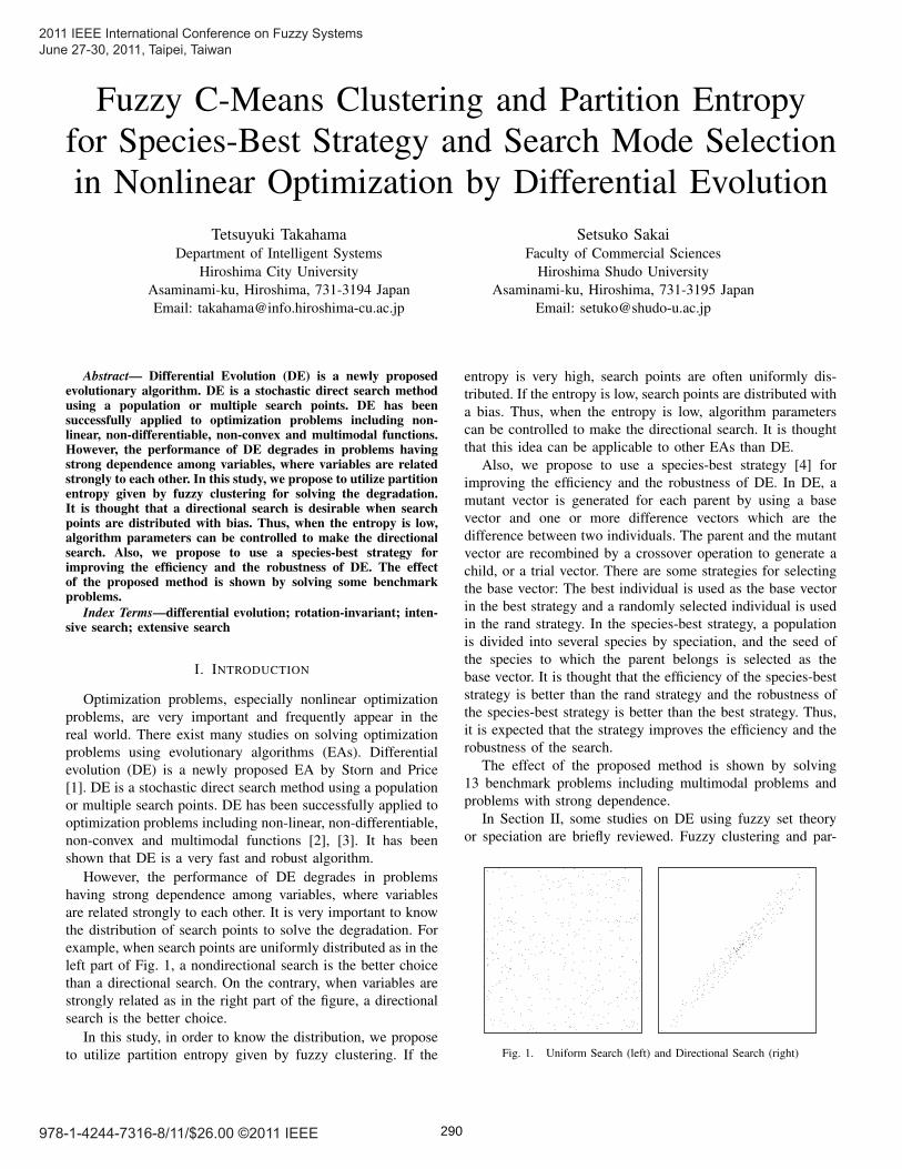
However, the performance of DE degrades in problemshaving strong dependence among variables, where variablesare related strongly to each other. It is very important to knowthe distribution of search points to solve the degradation. Forexample, when search points are uniformly distributed as in theleft part of Fig. 1, a nondirectional search is the better choicethan a directional search. On the contrary, when variables arestrongly related as in the right part of the figure, a directionalsearch is the better choice.

In this study, in order to know the distribution, we proposeto utilize partition entropy given by fuzzy clustering. If the

entropy is very high, search points are often uniformly dis-tributed. If the entropy is low, search points are distributed witha bias. Thus, when the entropy is low, algorithm parameterscan be controlled to make the directional search. It is thoughtthat this idea can be applicable to other EAs than DE.

Also, we propose to use a species-best strategy [4] forimproving the efficiency and the robustness of DE. In DE, amutant vector is generated for each parent by using a basevector and one or more difference vectors which are thedifference between two individuals. The parent and the mutantvector are recombined by a crossover operation to generate achild, or a trial vector. There are some strategies for selectingthe base vector: The best individual is used as the base vectorin the best strategy and a randomly selected individual is usedin the rand strategy. In the species-best strategy, a populationis divided into several species by speciation, and the seed ofthe species to which the parent belongs is selected as thebase vector. It is thought that the efficiency of the species-beststrategy is better than the rand strategy and the robustness ofthe species-best strategy is better than the best strategy. Thus,it is expected that the strategy improves the efficiency and therobustness of the search.

The effect of the proposed method is shown by solving13 benchmark problems including multimodal problems andproblems with strong dependence.

In Section II, some studies on DE using fuzzy set theoryor speciation are briefly reviewed. Fuzzy clustering and par-

Fig. 1. Uniform Search (left) and Directional Search (right)

290

tition entropy are explained in Section III. DE and DE withspeciation using fuzzy clustering are described in Section IVand V, respectively. In Section VI, experimental results onsome problems are shown. Finally, conclusions are describedin Section VII.

II. PREVIOUS WORKS

In this section, the optimization problem in this study isdefined and some studies on DE using fuzzy set theory orspeciation are described.

A. Optimization Problems

In this study, the following optimization problem with lowerbound and upper bound constraints will be discussed.

minimize f(x)subject to li ≤ xi ≤ ui, i = 1, . . . , D,

(1)

where x = (x1, x2, · · · , xD) is a D dimensional vector andf(x) is an objective function. The function f is a nonlinearreal-valued function. Values li and ui are the lower boundand the upper bound of xi, respectively. Let the search spacein which every point satisfies the lower and upper boundconstraints be denoted by S.

B. Fuzzy Set Theory

There exist some studies on optimization by DE using fuzzyset theory.

• Fuzzy logic: Fuzzy logic is used to control the parametersof DE. The fuzzy adaptive differential evolution (FADE)[5] is proposed to control parameters for a mutationoperation and a crossover operation. In each generation,the movement of individuals (vectors) and the change offunction values over the whole population between thelast two generations were nonlinearly depressed and usedas the inputs for fuzzy logic controllers.

• Fuzzy clustering: The hybrid DE based on fuzzy c-meansclustering (FCDE) [6] is proposed, which uses the one-step fuzzy c-means clustering. The clustering acts as amulti-parent crossover operation to utilize the informationof a population efficiently. In [7], fuzzy clusteringis used to divide a population into several clusters orniches, which are a kind of species described below, formultimodal optimization.

C. Speciation

Speciation is mainly used for multimodal optimizationwhere multiple optimal or suboptimal solutions are obtainedsimultaneously in one run. Each species evolves to find anoptimal or suboptimal solution. There exist some types ofresearch using speciation in DE [8].

• Radius-based speciation: In this category, a population issorted in increasing objective value order, first. Then, thebest individual in the sorted population becomes a newspecies seed. The population members that exist withinthe specified radius from the seed are assigned to thespecies, and the members are deleted from the population.

This process is repeated until the population becomesempty [4], [9], [10].

• Clustering-based speciationA population is divided into several clusters using aclustering algorithm such as k-means clustering [11] orfuzzy c-means clustering [7]. Each cluster correspondsto a species. If the seed of a species is necessary, anindividual that has the best objective value in the speciesis selected as the seed.

In this study, the clustering-based speciation using fuzzy c-means clustering is used not to multimodal optimization butto usual optimization for finding one optimal solution andimproving the efficiency of DE using the species-best strategy.Also, as a quite new approach, the partition entropy obtainedby the clustering is used to control the parameter for crossoveroperation of DE.

III. FUZZY C-MEANS CLUSTERING AND ENTROPY

In this section, fuzzy c-means clustering and partitionentropy are briefly explained [7], [12].

A. Fuzzy Partition and Partition Entropy

Fuzzy partition allows a data point to belong to two or moreclusters. Let X = {x1,x2, · · · ,xN} be a set of N data points.A fuzzy partition of X into C clusters can be defined with amatrix U = {µij}, 1 ≤ i ≤ N, 1 ≤ j ≤ C, which satisfies thefollowing conditions:

µij ∈ [0, 1] (2)C∑

j=1

µij = 1, 1 ≤ i ≤ N (3)

0 <N∑i=1

µij < N, 1 ≤ j ≤ C (4)

where µij is the degree of membership of the i-th data xi

in the j-th cluster. The higher µij indicates that the i-th databelongs to the j-th cluster more strongly.

Some evaluation criteria for the fuzzy partition are proposedsuch as partition entropy and so on. The normalized partitionentropy is defined as follows:

PE(C) = − 1

N log2 C

N∑i=1

C∑j=1

µij log2 µij (5)

where 0 ≤ PE(C) ≤ 1. The minimum value 0 correspondsto a hard partition, where each data point xi belongs to onlya cluster ci:

µij =

{1 j = ci0 j 6= ci

, 1 ≤ i ≤ N (6)

The maximum value 1 corresponds to the fuzziest partition,where each data point belongs to all clusters equivalently:

µij =1

C, 1 ≤ i ≤ N, 1 ≤ j ≤ C (7)

In this study, the entropy is used to detect the distributionof search points and alter the mode of the search by DE.

291

B. Fuzzy C-Means Clustering

Fuzzy C-Means (FCM) is a clustering method which re-alizes the fuzzy partition. This method is frequently usedin pattern recognition. The FCM algorithm minimizes thefollowing function:

Jm(U, V ) =

N∑i=1

C∑j=1

(µij)m||xi − vj ||2, 1 ≤ m <∞ (8)

where m is a real number parameter specifying degree of fuzzi-ness, vj is the center of the j-th cluster, V = {v1,v2, · · · ,vC}is a set of the cluster centers, and || · || represents any normexpressing the distance between a data point and the clustercenter.

The FCM algorithm is as follows:1) Assign membership values µij of all data in all clusters

randomly.2) Update cluster centers.

vj =

∑Ni=1(µij)

mxi∑Ni=1(µij)m

(9)

3) Update membership degrees.

µij =1∑C

k=1

(||xi−vj ||2||xi−vk||2

) 1m−1

(10)

4) The algorithm is terminated, when the following condi-tion is satisfied, or the change of membership degreesbetween two iterations is no more than ε, the givensensitivity threshold.

N∑i=1

C∑j=1

(µmij (t)− µm

ij (t− 1))2 ≤ ε (11)

where µmij (t) and µm

ij (t− 1) are the value at the currentiteration and that at the previous iteration, respectively.

5) Go back to 2).This algorithm minimizes intra-cluster variance, but the mini-mum is a local minimum and the results depend on the initialchoice of membership degrees.

IV. DIFFERENTIAL EVOLUTION

In this section, the outline of DE is described.

A. Outline of Differential Evolution

In DE, initial individuals are randomly generated withinthe given search space and form an initial population. Eachindividual contains D genes as decision variables. At eachgeneration or iteration, all individuals are selected as parents.Each parent is processed as follows: The mutation operationbegins by choosing several individuals from the populationexcept for the parent in the processing. The first individualis a base vector. All subsequent individuals are paired tocreate difference vectors. The difference vectors are scaled bya scaling factor F and added to the base vector. The resultingvector, or a mutant vector, is then recombined with the parent.The probability of recombination at an element is controlled

by a crossover rate CR. This crossover operation produces atrial vector. Finally, for survivor selection, the trial vector isaccepted for the next generation if the trial vector is better thanthe parent.

There are some variants of DE that have been proposed. Thevariants are classified using the notation DE/base/num/crosssuch as DE/rand/1/bin and DE/rand/1/exp.

“base” specifies a way of selecting an individual thatwill form the base vector. For example, DE/rand selects anindividual for the base vector at random from the population.DE/best selects the best individual in the population.

“num” specifies the number of difference vectors used toperturb the base vector. In case of DE/rand/1, for example, foreach parent xi, three individuals xp1, xp2 and xp3 are chosenrandomly from the population without overlapping xi and eachother. A new vector, or a mutant vector x′ is generated by thebase vector xp1 and the difference vector xp2−xp3, where Fis the scaling factor.

x′ = xp1 + F (xp2 − xp3) (12)

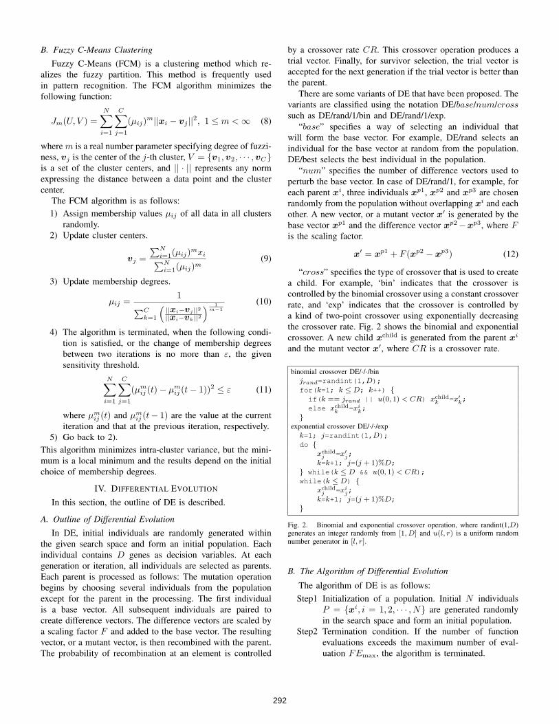
“cross” specifies the type of crossover that is used to createa child. For example, ‘bin’ indicates that the crossover iscontrolled by the binomial crossover using a constant crossoverrate, and ‘exp’ indicates that the crossover is controlled bya kind of two-point crossover using exponentially decreasingthe crossover rate. Fig. 2 shows the binomial and exponentialcrossover. A new child xchild is generated from the parent xi

and the mutant vector x′, where CR is a crossover rate.

binomial crossover DE/·/·/binjrand=randint(1,D);for(k=1; k ≤ D; k++) {if(k == jrand || u(0, 1) < CR) xchild

k =x′k;

else xchildk =xi

k;}

exponential crossover DE/·/·/expk=1; j=randint(1,D);do {

xchildj =x′

j;k=k+1; j=(j + 1)%D;

} while(k ≤ D && u(0, 1) < CR);while(k ≤ D) {

xchildj =xi

j;k=k+1; j=(j + 1)%D;

}

Fig. 2. Binomial and exponential crossover operation, where randint(1,D)generates an integer randomly from [1, D] and u(l, r) is a uniform randomnumber generator in [l, r].

B. The Algorithm of Differential Evolution

The algorithm of DE is as follows:Step1 Initialization of a population. Initial N individuals

P = {xi, i = 1, 2, · · · , N} are generated randomlyin the search space and form an initial population.

Step2 Termination condition. If the number of functionevaluations exceeds the maximum number of eval-uation FEmax, the algorithm is terminated.

292

Step3 DE operations. Each individual xi is selected as aparent. If all individuals are selected, go to Step4. Amutant vector x′ is generated according to Eq. (12).A trial vector (child) is generated from the parent xi

and the mutant vector x′ using a crossover operationshown in Fig. 2. If the child is better than or equal tothe parent, or the DE operation is succeeded, the childsurvives. Otherwise the parent survives. Go back toStep3 and the next individual is selected as a parent.

Step4 Survivor selection (generation change). The popula-tion is organized by the survivors. Go back to Step2.

Fig. 3 shows a pseudo-code of DE/rand/1.

DE/rand/1(){// Initialize a populationP=N individuals generated randomly in S;for(t=1; FE ≤ FEmax; t++) {for(i=1; i ≤ N; i++) {

// DE operationsxp1=Randomly selected from P(p1 6= i);xp2=Randomly selected from P(p2 6∈ {i, p1});xp3=Randomly selected from P(p3 6∈ {i, p1, p2});x′=xp1+F (xp2 − xp3);xchild=trial vector is generated from

xi and x′ by the crossover operation;// Survivor selection

if(f(xchild)≤ f(xi)

)zi=xchild;

else zi=xi;FE=FE+1;

}P={zi, i = 1, 2, · · · , N};

}}

Fig. 3. The pseudo-code of DE, FE is the number of function evaluations.

V. DE WITH SPECIATION USING FUZZY CLUSTERING

In this section, DE with speciation using fuzzy clustering(DESFC) is proposed.

A. Species-Best Strategy

The following steps are executed in each generation torealize the species-best strategy.

1) FCM is applied to a population P = {x1,x2, · · · ,xN}where N is the population size. The membership gradeof the i-th individual xi in the j-th cluster, µij , 1 ≤ i ≤N , 1 ≤ j ≤ C is obtained where C is the number ofclusters.

2) Each cluster j corresponds to one species. The i-thindividual is assigned to the cluster or the species Si

where µij has the maximum value.

Si = arg max1≤j≤C

µij , 1 ≤ i ≤ N (13)

3) The seed of j-th species, seedj is the best individual inthe species.

seedj = arg min{i|Si=j}

f(xi), 1 ≤ j ≤ C (14)

Thus, the seed for the i-th individual can be obtained asseedSi .

The species-best strategy to xi can be described as follows:

x′ = xseedSi + F (xp2 − xp3) (15)

where p2 and p3 are random integers in [1, N ] and i, p2 andp3 are different with each other.

B. Algorithm of DESFC

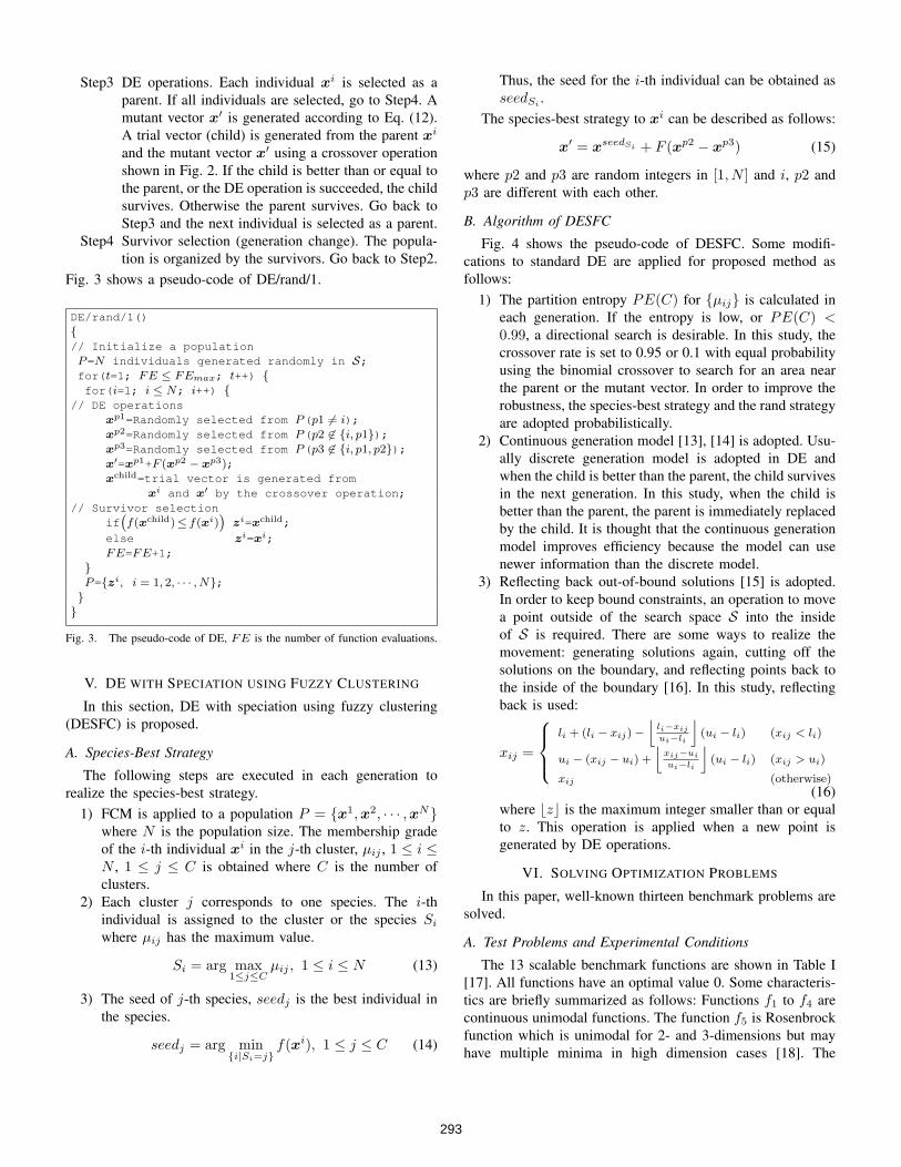
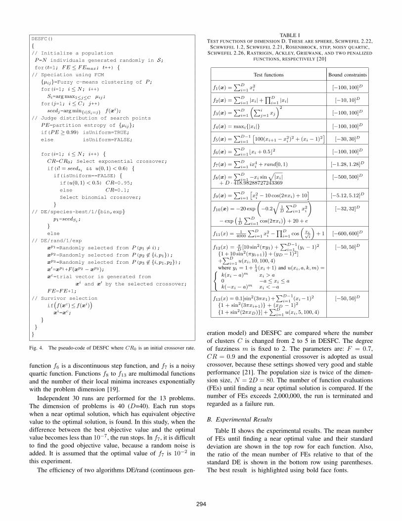
Fig. 4 shows the pseudo-code of DESFC. Some modifi-cations to standard DE are applied for proposed method asfollows:

1) The partition entropy PE(C) for {µij} is calculated ineach generation. If the entropy is low, or PE(C) <0.99, a directional search is desirable. In this study, thecrossover rate is set to 0.95 or 0.1 with equal probabilityusing the binomial crossover to search for an area nearthe parent or the mutant vector. In order to improve therobustness, the species-best strategy and the rand strategyare adopted probabilistically.

2) Continuous generation model [13], [14] is adopted. Usu-ally discrete generation model is adopted in DE andwhen the child is better than the parent, the child survivesin the next generation. In this study, when the child isbetter than the parent, the parent is immediately replacedby the child. It is thought that the continuous generationmodel improves efficiency because the model can usenewer information than the discrete model.

3) Reflecting back out-of-bound solutions [15] is adopted.In order to keep bound constraints, an operation to movea point outside of the search space S into the insideof S is required. There are some ways to realize themovement: generating solutions again, cutting off thesolutions on the boundary, and reflecting points back tothe inside of the boundary [16]. In this study, reflectingback is used:

xij =

li + (li − xij)−

⌊li−xij

ui−li

⌋(ui − li) (xij < li)

ui − (xij − ui) +

⌊xij−ui

ui−li

⌋(ui − li) (xij > ui)

xij (otherwise)(16)

where bzc is the maximum integer smaller than or equalto z. This operation is applied when a new point isgenerated by DE operations.

VI. SOLVING OPTIMIZATION PROBLEMS

In this paper, well-known thirteen benchmark problems aresolved.

A. Test Problems and Experimental Conditions

The 13 scalable benchmark functions are shown in Table I[17]. All functions have an optimal value 0. Some characteris-tics are briefly summarized as follows: Functions f1 to f4 arecontinuous unimodal functions. The function f5 is Rosenbrockfunction which is unimodal for 2- and 3-dimensions but mayhave multiple minima in high dimension cases [18]. The

293

DESFC()

{// Initialize a population

P=N individuals generated randomly in S;for(t=1; FE ≤ FEmax; t++) {// Speciation using FCM

{µij}=Fuzzy c-means clustering of P;

for(i=1; i ≤ N; i++)

Si=argmax1≤j≤C µij;

for(j=1; i ≤ C; j++)

seedj=argmin{i|Si=j} f(xi);

// Judge distribution of search points

PE=partition entropy of {µij};if(PE ≥ 0.99) isUniform=TRUE;

else isUniform=FALSE;

for(i=1; i ≤ N; i++) {CR=CR0; Select exponential crossover;

if(i! = seedsi && u(0, 1) < 0.6) {if(isUniform==FALSE) {if(u(0, 1) < 0.5) CR=0.95;

else CR=0.1;

Select binomial crossover;

}// DE/species-best/1/{bin,exp}

p1=seedSi;

}else

// DE/rand/1/exp

xp1=Randomly selected from P(p1 6= i);

xp2=Randomly selected from P(p2 6∈ {i, p1});xp3=Randomly selected from P(p3 6∈ {i, p1, p2});x′=xp1+F (xp2 − xp3 );

xc=trial vector is generated from

xi and x′ by the selected crossover;

FE=FE+1;

// Survivor selection

if(f(xc)≤ f(xi)

)xi=xc;

}}

}

Fig. 4. The pseudo-code of DESFC where CR0 is an initial crossover rate.

function f6 is a discontinuous step function, and f7 is a noisyquartic function. Functions f8 to f13 are multimodal functionsand the number of their local minima increases exponentiallywith the problem dimension [19].

Independent 30 runs are performed for the 13 problems.The dimension of problems is 40 (D=40). Each run stopswhen a near optimal solution, which has equivalent objectivevalue to the optimal solution, is found. In this study, when thedifference between the best objective value and the optimalvalue becomes less than 10−7, the run stops. In f7, it is difficultto find the good objective value, because a random noise isadded. It is assumed that the optimal value of f7 is 10−2 inthis experiment.

The efficiency of two algorithms DE/rand (continuous gen-

TABLE ITEST FUNCTIONS OF DIMENSION D. THESE ARE SPHERE, SCHWEFEL 2.22,

SCHWEFEL 1.2, SCHWEFEL 2.21, ROSENBROCK, STEP, NOISY QUARTIC,SCHWEFEL 2.26, RASTRIGIN, ACKLEY, GRIEWANK, AND TWO PENALIZED

FUNCTIONS, RESPECTIVELY [20]

Test functions Bound constraints

f1(x) =∑D

i=1x2i [−100, 100]D

f2(x) =∑D

i=1|xi|+

∏D

i=1|xi| [−10, 10]D

f3(x) =∑D

i=1

(∑i

j=1xj

)2

[−100, 100]D

f4(x) = maxi{|xi|} [−100, 100]D

f5(x) =∑D−1

i=1

[100(xi+1 − x2

i )2 + (xi − 1)2

][−30, 30]D

f6(x) =∑D

i=1bxi + 0.5c2 [−100, 100]D

f7(x) =∑D

i=1ix4

i + rand[0, 1) [−1.28, 1.28]D

f8(x) =∑D

i=1−xi sin

√|xi|

+D · 418.98288727243369[−500, 500]D

f9(x) =∑D

i=1

[x2i − 10 cos(2πxi) + 10

][−5.12, 5.12]D

f10(x) = −20 exp

(−0.2

√1D

∑D

i=1x2i

)− exp

(1D

∑D

i=1cos(2πxi)

)+ 20 + e

[−32, 32]D

f11(x) =1

4000

∑D

i=1x2i −∏D

i=1cos

(xi√i

)+ 1 [−600, 600]D

f12(x) = πD[10 sin2(πy1) +

∑D−1

i=1(yi − 1)2

{1+ 10 sin2(πyi+1)}+(yD − 1)2]

+∑D

i=1u(xi, 10, 100, 4)

where yi = 1+ 14(xi +1) and u(xi, a, k,m) ={

k(xi − a)m xi > a0 −a ≤ xi ≤ ak(−xi − a)m xi < −a

[−50, 50]D

f13(x) = 0.1[sin2(3πx1)+∑D−1

i=1(xi−1)2

{1 + sin2(3πxi+1)} + (xD − 1)2

{1 + sin2(2πxD)}] +∑D

i=1u(xi, 5, 100, 4)

[−50, 50]D

eration model) and DESFC are compared where the numberof clusters C is changed from 2 to 5 in DESFC. The degreeof fuzziness m is fixed to 2. The parameters are: F = 0.7,CR = 0.9 and the exponential crossover is adopted as usualcrossover, because these settings showed very good and stableperformance [21]. The population size is twice of the dimen-sion size, N = 2D = 80. The number of function evaluations(FEs) until finding a near optimal solution is compared. If thenumber of FEs exceeds 2,000,000, the run is terminated andregarded as a failure run.

B. Experimental Results

Table II shows the experimental results. The mean numberof FEs until finding a near optimal value and their standarddeviation are shown in the top row for each function. Also,the ratio of the mean number of FEs relative to that of thestandard DE is shown in the bottom row using parentheses.The best result is highlighted using bold face fonts.

294

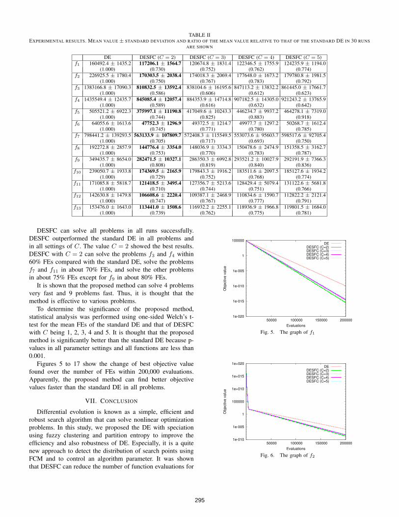
TABLE IIEXPERIMENTAL RESULTS. MEAN VALUE ± STANDARD DEVIATION AND RATIO OF THE MEAN VALUE RELATIVE TO THAT OF THE STANDARD DE IN 30 RUNS

ARE SHOWN

DE DESFC (C = 2) DESFC (C = 3) DESFC (C = 4) DESFC (C = 5)f1 160492.4 ± 1435.2 117206.1 ± 1564.7 120674.8 ± 1831.4 122346.5 ± 1755.9 124235.9 ± 1194.0

(1.000) (0.730) (0.752) (0.762) (0.774)f2 226925.5 ± 1780.4 170303.5 ± 2038.4 174018.3 ± 2069.4 177648.0 ± 1673.2 179780.8 ± 1981.5

(1.000) (0.750) (0.767) (0.783) (0.792)f3 1383166.8 ± 17090.3 810832.5 ± 13592.4 838104.6 ± 16195.6 847113.2 ± 13832.2 861445.0 ± 17661.7

(1.000) (0.586) (0.606) (0.612) (0.623)f4 1435549.4 ± 12435.7 845085.4 ± 12057.4 884353.9 ± 14714.8 907182.5 ± 14305.0 921243.2 ± 13765.9

(1.000) (0.589) (0.616) (0.632) (0.642)f5 505521.2 ± 6922.3 375997.1 ± 11190.8 417049.6 ± 10243.3 446234.7 ± 9937.2 464278.1 ± 7319.0

(1.000) (0.744) (0.825) (0.883) (0.918)f6 64055.6 ± 1613.6 47752.3 ± 1296.9 49372.5 ± 1214.7 49977.7 ± 1297.2 50268.7 ± 1612.4

(1.000) (0.745) (0.771) (0.780) (0.785)f7 798441.2 ± 139293.5 563133.9 ± 107809.7 572408.3 ± 115549.5 553073.6 ± 95603.7 598517.6 ± 92705.4

(1.000) (0.705) (0.717) (0.693) (0.750)f8 192272.8 ± 2857.9 144776.4 ± 3354.0 148036.9 ± 3334.3 150478.6 ± 2474.9 151358.5 ± 3162.7

(1.000) (0.753) (0.770) (0.783) (0.787)f9 349435.7 ± 8654.0 282471.5 ± 10327.1 286350.3 ± 6992.8 293521.2 ± 10027.9 292191.9 ± 7366.3

(1.000) (0.808) (0.819) (0.840) (0.836)f10 239050.7 ± 1933.8 174369.5 ± 2165.9 179843.3 ± 1916.2 183511.6 ± 2097.5 185127.6 ± 1934.2

(1.000) (0.729) (0.752) (0.768) (0.774)f11 171085.8 ± 5818.7 121418.5 ± 3495.4 127356.7 ± 5213.6 128429.4 ± 5079.4 131122.6 ± 5681.8

(1.000) (0.710) (0.744) (0.751) (0.766)f12 142630.8 ± 1479.8 106608.6 ± 2220.4 109387.1 ± 2468.9 110834.6 ± 1590.7 112822.2 ± 2121.4

(1.000) (0.747) (0.767) (0.777) (0.791)f13 153476.0 ± 1643.0 113441.0 ± 1508.6 116932.2 ± 2255.1 118936.9 ± 1966.8 119801.5 ± 1684.0

(1.000) (0.739) (0.762) (0.775) (0.781)

DESFC can solve all problems in all runs successfully.DESFC outperformed the standard DE in all problems andin all settings of C. The value C = 2 showed the best results.DESFC with C = 2 can solve the problems f3 and f4 within60% FEs compared with the standard DE, solve the problemsf7 and f11 in about 70% FEs, and solve the other problemsin about 75% FEs except for f9 in about 80% FEs.

It is shown that the proposed method can solve 4 problemsvery fast and 9 problems fast. Thus, it is thought that themethod is effective to various problems.

To determine the significance of the proposed method,statistical analysis was performed using one-sided Welch’s t-test for the mean FEs of the standard DE and that of DESFCwith C being 1, 2, 3, 4 and 5. It is thought that the proposedmethod is significantly better than the standard DE because p-values in all parameter settings and all functions are less than0.001.

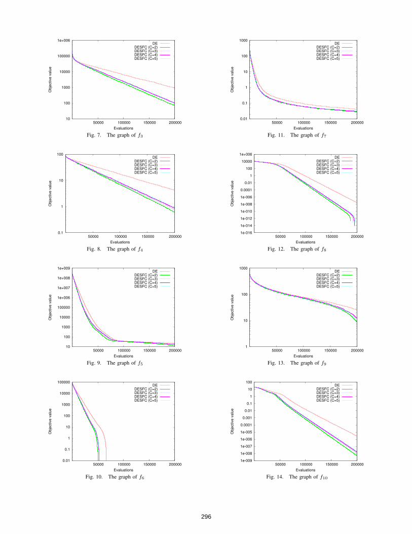
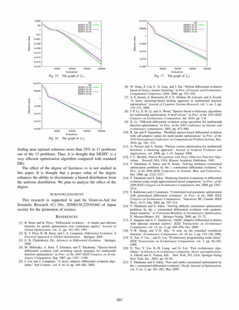
Figures 5 to 17 show the change of best objective valuefound over the number of FEs within 200,000 evaluations.Apparently, the proposed method can find better objectivevalues faster than the standard DE in all problems.

VII. CONCLUSION

Differential evolution is known as a simple, efficient androbust search algorithm that can solve nonlinear optimizationproblems. In this study, we proposed the DE with speciationusing fuzzy clustering and partition entropy to improve theefficiency and also robustness of DE. Especially, it is a quitenew approach to detect the distribution of search points usingFCM and to control an algorithm parameter. It was shownthat DESFC can reduce the number of function evaluations for

1e-020

1e-015

1e-010

1e-005

1

100000

50000 100000 150000 200000

Ob

jective

va

lue

Evaluations

DEDESFC (C=2)DESFC (C=3)DESFC (C=4)DESFC (C=5)

Fig. 5. The graph of f1

1e-010

1e-005

1

100000

1e+010

1e+015

1e+020

50000 100000 150000 200000

Ob

jective

va

lue

Evaluations



295

10

100

1000

10000

100000

1e+006

50000 100000 150000 200000

Ob

jective

va

lue

Evaluations



0.1

1

10

100

50000 100000 150000 200000

Ob

jective

va

lue

Evaluations



10

100

1000

10000

100000

1e+006

1e+007

1e+008

1e+009

50000 100000 150000 200000

Ob

jective

va

lue

Evaluations



0.01

0.1

1

10

100

1000

10000

100000

50000 100000 150000 200000

Ob

jective

va

lue

Evaluations



0.01

0.1

1

10

100

1000

50000 100000 150000 200000

Ob

jective

va

lue

Evaluations



1e-016

1e-014

1e-012

1e-010

1e-008

1e-006

0.0001

0.01

1

100

10000

1e+006

50000 100000 150000 200000O

bje

ctive

va

lue

Evaluations



1

10

100

1000

50000 100000 150000 200000

Ob

jective

va

lue

Evaluations



1e-009

1e-008

1e-007

1e-006

1e-005

0.0001

0.001

0.01

0.1

1

10

100

50000 100000 150000 200000

Ob

jective

va

lue

Evaluations



296

1e-016

1e-014

1e-012

1e-010

1e-008

1e-006

0.0001

0.01

1

100

10000

50000 100000 150000 200000

Ob

jective

va

lue

Evaluations



1e-020

1e-015

1e-010

1e-005

1

100000

1e+010

50000 100000 150000 200000

Ob

jective

va

lue

Evaluations



finding near optimal solutions more than 25% in 11 problemsout of the 13 problems. Thus, it is thought that DESFC is avery efficient optimization algorithm compared with standardDEs.

The effect of the degree of fuzziness m is not studied inthis paper. It is thought that a proper value of the degreeenhances the ability to discriminate a biased distribution fromthe uniform distribution. We plan to analyze the effect of thedegree.

ACKNOWLEDGMENT

This research is supported in part by Grant-in-Aid forScientific Research (C) (No. 20500138,22510166) of Japansociety for the promotion of science.

REFERENCES

[1] R. Storn and K. Price, “Differential evolution – A simple and efficientheuristic for global optimization over continuous spaces,” Journal ofGlobal Optimization, vol. 11, pp. 341–359, 1997.

[2] K. V. Price, R. M. Storn, and J. A. Lampinen, Differential Evolution: APractical Approach to Global Optimization. Springer, 2005.

[3] U. K. Chakraborty, Ed., Advances in Differential Evolution. Springer,2008.

[4] M. Shibasaka, A. Hara, T. Ichimura, and T. Takahama, “Species-baseddifferential evolution with switching search strategies for multimodalfunction optimization,” in Proc. of the 2007 IEEE Congress on Evolu-tionary Computation, Sep. 2007, pp. 1183 –1190.

[5] J. Liu and J. Lampinen, “A fuzzy adaptive differential evolution algo-rithm,” Soft Comput., vol. 9, no. 6, pp. 448–462, 2005.

1e-020

1e-015

1e-010

1e-005

1

100000

1e+010

50000 100000 150000 200000

Ob

jective

va

lue

Evaluations



[6] W. Gong, Z. Cai, C. X. Ling, and J. Du, “Hybrid differential evolutionbased on fuzzy c-means clustering,” in Proc. of Genetic and EvolutionaryComputation Conference 2009, 2009, pp. 523–530.

[7] A. E. Imrani, A. Bouroumi, H. Z. E. Abidine, M. Limouri, and A. Essaı̈d,“A fuzzy clustering-based niching approach to multimodal functionoptimization,” Journal of Cognitive Systems Research, vol. 1, no. 2, pp.119–133, 2000.

[8] J.-P. Li, X.-D. Li, and A. Wood, “Species based evolutionary algorithmsfor multimodal optimization: A brief review,” in Proc. of the 2010 IEEECongress on Evolutionary Computation, Jul. 2010, pp. 1–8.

[9] X. Li, “Efficient differential evolution using speciation for multimodalfunction optimization,” in Proc. of the 2005 conference on Genetic andevolutionary computation, 2005, pp. 873–880.

[10] B. Qu and P. Suganthan, “Modified species-based differential evolutionwith self-adaptive radius for multi-modal optimization,” in Proc. of the2010 International Conference on Computational Problem-Solving, Dec.2010, pp. 326 –331.

[11] A. Passaro and A. Starita, “Particle swarm optimization for multimodalfunctions: a clustering approach,” Journal of Artificial Evolution andApplications, vol. 2008, pp. 1–15, January 2008.

[12] J. C. Bezdek, Pattern Recognition with Fuzzy Objective Function Algo-rithms. Norwell, MA, USA: Kluwer Academic Publishers, 1981.

[13] T. Takahama, S. Sakai, and N. Iwane, “Solving nonlinear constrainedoptimization problems by the ε constrained differential evolution,” inProc. of the 2006 IEEE Conference on Systems, Man, and Cybernetics,Oct. 2006, pp. 2322–2327.

[14] T. Takahama and S. Sakai, “Reducing function evaluations in differentialevolution using rough approximation-based comparison,” in Proc. of the2008 IEEE Congress on Evolutionary Computation, Jun. 2008, pp. 2307–2314.

[15] S. Kukkonen and J. Lampinen, “Constrained real-parameter optimizationwith generalized differential evolution,” in Proc. of the 2006 IEEECongress on Evolutionary Computation. Vancouver, BC, Canada: IEEEPress, 16-21 July 2006, pp. 207–214.

[16] T. Takahama and S. Sakai, “Solving difficult constrained optimizationproblems by the ε constrained differential evolution with gradient-based mutation,” in Constraint-Handling in Evolutionary Optimization,E. Mezura-Montes, Ed. Springer-Verlag, 2009, pp. 51–72.

[17] Z. Jingqiao and A. C. Sanderson, “JADE: Adaptive differential evolutionwith optional external archive,” IEEE Transactions on EvolutionaryComputation, vol. 13, no. 5, pp. 945–958, Oct. 2009.

[18] Y.-W. Shang and Y.-H. Qiu, “A note on the extended rosenbrockfunction,” Evolutionary Computation, vol. 14, no. 1, pp. 119–126, 2006.

[19] X. Yao, Y. Liu, , and G. Lin, “Evolutionary programming made faster,”IEEE Transactions on Evolutionary Computation, vol. 3, pp. 82–102,1999.

[20] X. Yao, Y. Liu, K.-H. Liang, and G. Lin, “Fast evolutionary algo-rithms,” in Advances in evolutionary computing: theory and applications,A. Ghosh and S. Tsutsui, Eds. New York, NY, USA: Springer-VerlagNew York, Inc., 2003, pp. 45–94.

[21] T. Takahama and S. Sakai, “Fast and stable constrained optimization bythe ε constrained differential evolution,” Pacific Journal of Optimization,vol. 5, no. 2, pp. 261–282, May 2009.

297

June 27-30, 2011, Taipei, Taiwan Fuzzy C-Means Clustering ...

Documents

Transcript of June 27-30, 2011, Taipei, Taiwan Fuzzy C-Means Clustering ...